The origin of very-high-energy gamma-rays from GRB 221009A: implications for reverse shock proton synchrotron emission

Abstract

Recently, GRB 221009A, known as the brightest of all time (BOAT), has been observed across an astounding range of $\sim 18$ orders of magnitude in energy, spanning from radio to VHE bands. Notably, the Large High Altitude Air Shower Observatory (LHAASO) recorded over $60000$ photons with energies exceeding $0.2\rm~{}TeV$, including the first-ever detection of photons above $10\rm~{}TeV$. However, explaining the observed energy flux evolution in the VHE band alongside late-time multi-wavelength data poses a significant challenge. Our approach involves a two-component structured jet model, consisting of a narrow core dominated by magnetic energy and a wide jet component dominated by matter. We show that the combination of the forward shock electron synchrotron self-Compton emission from both jets and reverse shock proton synchrotron emission from the wide jet could account for both the energy flux and spectral evolution in the VHE band, and the early TeV lightcurve may be influenced by prompt photons which could explain the initial steep rising phase. We noticed the arrival time of the highest energy photons detected by LHAASO-KM2A coincident with the peak of the reverse shock proton synchrotron emission, especially a minor flare occurring about $\sim 500-800$ seconds after the trigger, coinciding with the observed spectral hardening and arrival time of the $\sim 13\rm~{}TeV$ photons detected by LHAASO. These findings imply that the GRB reverse shock may serve as a potential accelerator of ultra-high-energy cosmic rays, a hypothesis that could be tested through future multimessenger observations.

1 Introduction

The detection of very-high-energy (VHE) gamma-rays (with energies ranging from 0.1 TeV to 100 TeV) originating from gamma-ray bursts (GRBs) marks a significant advancement in our ability to explore the physics of GRBs and their associated radiative processes (See Mészáros, 2006; Kumar & Zhang, 2014; Zhang, 2018, for a review). The initial detections in the VHE band included GRB 190114C observed by the Major Atmospheric Gamma Imaging Cherenkov (MAGIC) telescopes (Acciari et al., 2019a, b) and GRB 180721B observed by the High Energy Stereoscopic System (H.E.S.S.) (Abdalla et al., 2019). Subsequently, VHE gamma-rays from GRB 190829A (Abdalla et al., 2021) and GRB 201216C (Blanch et al., 2020b) were also reported. Furthermore, there are two sub-threshold events, namely GRB 160821B (Acciari et al., 2021) and GRB 201015A (Blanch et al., 2020a). The four significantly detected VHE GRBs are long GRBs (Noda & Parsons, 2022). All these detections align with the hypothesis that VHE gamma-rays originate during the afterglow phase when the relativistic outflow enters the self-similar deceleration phase (Zhang, 2019; Miceli & Nava, 2022). However, it’s worth noting that both MAGIC and H.E.S.S. operate as Imaging Atmospheric Cherenkov Telescopes (IACTs), characterized by limited fields of view and the necessity for longer slew times to perform follow-up observations. Consequently, the detection of VHE gamma-rays from the early afterglow, especially during the prompt phase, presents a formidable challenge.

On October 9, 2022, the Fermi Gamma-ray Burst Monitor (Fermi-GBM) detected GRB 221009A at $T_{0}$ = 13:16:59.99 UT (Lesage et al., 2023). Because of its proximity, GRB 221009A has been referred to as the brightest of all time (BOAT) (Burns et al., 2023). Furthermore, this GRB was also captured by the Large High Altitude Air Shower Observatory (LHAASO), an extensive air shower detector designed for gamma-ray observations (Ma et al., 2022). A detailed analysis of LHAASO’s Water Cherenkov Detector Array (WCDA) data unveiled more than $64000$ photons with energies ranging from 0.2 TeV to 7 TeV that can be attributed to GRB 221009A within the first $T-T_{0}\sim 3000$ seconds following the Fermi-GBM trigger at $T_{0}$ (Cao et al., 2023b). Moreover, the LHAASO-KM2A detector also registered dozens of photons with energies exceeding $\sim 7$ TeV, with the highest recorded photon energy surpassing 10 TeV (Cao et al., 2023a). Notably, the absence of VHE gamma-ray detection during the prompt phase imposes stringent constraints on prompt TeV emission. For the first time, we observed the rising phase of energy flux in the VHE band, which reached it peak flux at $T_{0}+244\rm~{}s$ and then gradually declined over time. This smooth temporal profile of the TeV light curve aligns with its origin in the afterglow phase (Cao et al., 2023b).

Multiple studies lend support to the idea that VHE gamma-rays originate during the afterglow phase. In this scenario, the standard one-zone synchrotron self-Compton (SSC) process plays a pivotal role in generating the observed VHE gamma-rays (Meszaros & Rees, 1994; Dermer et al., 2000; Sari & Esin, 2001; Zhang & Meszaros, 2001). In the SSC model, the same group of electrons responsible for synchrotron emission can upscatter these photons to higher energies by a factor of approximately $\gamma_{e}^{2}$, where $\gamma_{e}$ represents the electron Lorentz factor. This SSC framework has successfully explained the emissions observed in VHE GRBs (e.g., Acciari et al., 2019a; Abdalla et al., 2019; Wang et al., 2019; Asano et al., 2020; Derishev & Piran, 2021; Abdalla et al., 2021; Salafia et al., 2022; Sato et al., 2023a; Khangulyan et al., 2023b; Zhang et al., 2021b; Huang, 2022; Ren et al., 2023b; Sato et al., 2023b). Nevertheless, it remains unclear whether the SSC process is the sole mechanism responsible for producing VHE gamma-rays in GRBs. An alternative process that warrants consideration is the external inverse-Compton (EIC) mechanism, particularly in scenarios where the prompt emission coincides with the early afterglow phase (Wang et al., 2006; Murase et al., 2010; Toma et al., 2009; Murase et al., 2011; He et al., 2012; Veres & Mészáros, 2014; Murase et al., 2018). Recent studies lend credence to the EIC scenario as a viable alternative for VHE gamma-ray production, especially when considering the presence of a long-lasting central engine (Zhang et al., 2021a) and/or flares (Zhang et al., 2021c). The coherent jitter radiation in relativistic shock can also reach the VHE band (Ioka, 2006; Mao & Wang, 2023).

VHE gamma-ray production may also involve hadronic processes associated with the acceleration of cosmic ray protons and ions. In the realm of high-energy astrophysical sources featuring relativistic jets, extensive research has focused on proton synchrotron emission (e.g., Totani, 1998; Zhang & Meszaros, 2001; Murase et al., 2008; Asano et al., 2009) and photomeson production processes (e.g., Waxman & Bahcall, 2000). However, the absence of high-energy neutrinos from GRBs imposes stringent constraints on the efficiency of photomeson production process (e.g., Murase et al., 2022; Ai & Gao, 2023; Liu et al., 2023; Rudolph et al., 2023; Abbasi et al., 2023). Conversely, the radiative efficiency of the proton synchrotron process is considerably lower than that of electrons, necessitating the acceleration of protons to ultra-high-energies (UHE, exceeding $1\rm~{}EeV$). Isravel et al. (2023b) utilized synchrotron emission from UHE protons, accelerated within the external forward shock, to account for the observed VHE gamma-rays in GRB 190114C, with the SSC component in a subordinate role. Similarly, Huang et al. (2023) examined UHE protons accelerated during the prompt emission phase and injected into the afterglow jet, demonstrating that proton synchrotron emission could dominate the early TeV afterglow of GRB190829A. Inspired by the detection of $\gtrsim 10\rm~{}TeV$ photons from GRB 221009A, Zhang et al. (2023) put forward the idea that reverse shock proton synchrotron emission could be a significant contributor to VHE gamma-ray production in the case of GRB 221009A (See Isravel et al., 2023a, for the external forward shock model.).

Studying the production of VHE gamma-rays in detail is crucial, especially considering the remarkable TeV flux light curve observed by LHAASO and the wealth of multiwavelength data available. In their study Cao et al. (2023b), they conducted comprehensive numerical modeling of the TeV light curve, focusing on the time window covered by LHAASO’s observations. They assume that the emission originated from a narrow jet, with the late-time radio to GeV data attributed to a second jet (Sato et al., 2023b; Zheng et al., 2023). While the TeV light curve suggests a preference for a constant external medium density distribution (Cao et al., 2023b; Sato et al., 2023b), the late-time radio afterglow aligns with the propagation in a wind medium (Ren et al., 2023b; Gill & Granot, 2023). In our earlier work of  Zhang et al. (2023), we focused on the moment when the reverse shock has fully traversed the ejecta, marking the point at which the reverse shock emission attains its peak luminosity. Interestingly, our analysis revealed that proton synchrotron emission exhibits hard spectra, and the maximum energy of these emissions can surpass $10\rm~{}TeV$. However, Zhang et al. (2023) came out before the available of the LHAASO data and without considering the realistic dynamical evolution of the jet, so it is reasonable to perform detailed calculations of the reverse shock proton synchrotron model in this work.

In this study, we conduct comprehensive numerical modeling of VHE gamma-ray production and multiwavelength light curves using the standard reverse-forward external shock model with a structured jet. We investigate various radiative processes involving non-thermal electrons and protons from both the shocked ejecta and the shocked external medium. Our paper is organized as follows: In Section 2, we provide detailed information about the numerical modeling of the reverse-forward shock emission within the structured jet. In Section 3, we present our findings and compare them to the observed multi-wavelength light curves and energy spectra from GRB 221009A. In Section 4, we discuss the implications of our results. Finally, we summarize our study in Section 5.

In this study, we employ centimetre-gram-second system units and express quantities as $Q=Q_{x}10^{x}$. We denote photon energy in the observer frame as $E$ and in the comoving frame as $\varepsilon$.

2 Physical model

2.1 Structured jet

Structured jets in the context of GRBs have been extensively studied in previous research (Mészáros et al., 1998; Rossi et al., 2002; Zhang & Meszaros, 2002; Kumar & Granot, 2003; Zhang et al., 2004). The detection of the gravitational wave event GW 170817A (Abbott et al., 2017a) and the associated short GRB 170817A (Abbott et al., 2017b) provides a unique opportunity to explore the characteristics of relativistic jets. The gradually rising radio to X-ray afterglow observations supports the off-axis structured jet model (Lazzati et al., 2018; Margutti et al., 2018; Troja et al., 2018; Ioka & Nakamura, 2018). Structured jet formation is a natural outcome when the jet interacts with the stellar envelope (Gottlieb et al., 2020a, b). Interestingly, the TeV light curve fitting implies that the observed narrow jet corresponds to the core of the structured jet (Cao et al., 2023b). Furthermore, the observed X-ray decay rate is shallower than the predicted post jet-break index for a standard top-hat jet, suggesting that relativistic jets likely exhibit angular structure in their energy profiles (O’Connor et al., 2023; Gill & Granot, 2023).

In this study, we present an illustrative representation of a structured jet, which consists of a magnetic-dominated narrow core and a matter-dominated wide wing component, as depicted in Fig. 1. The magnetic-dominated narrow core is represented as a top-hat jet with a uniform energy and velocity distribution. Conversely, the matter-dominated wide jet component is modeled as a power-law structured jet.

We define $\mathcal{E}(\theta)$ as the angle-dependent isotropic-equivalent energy of a given structured jet. For the power-law structured jet, we have (e.g. Takahashi et al., 2022)

$$\mathcal{E}(\theta)=\mathcal{E}_{k}\left[1+\left(\frac{\theta}{\theta_{c}}\right)^{2}\right]^{-a/2}\ (\theta<\theta_{j}),$$ (1)

where $\mathcal{E}_{k}$ represents the isotropic-equivalent kinetic energy, $\theta_{c}$ is the narrow cone angle, $a$ is the power-law index, and $\theta_{j}$ is the jet half-opening angle. The distribution of the Lorentz factor is described as

$$\Gamma(\theta)=\Gamma_{0}\left[1+\left(\frac{\theta}{\theta_{c}}\right)^{2}\right]^{-a/2}\ (\theta<\theta_{j}),$$ (2)

where $\Gamma_{0}$ is the initial Lorentz factor. In the case of a uniform top-hat jet, $a=0$.

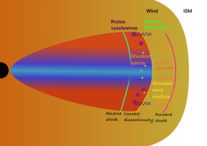
Figure 1: A schematic depiction of the structured jet, featuring a magnetic-energy-dominated narrow core (illustrated with blue color) and a matter-dominated wide jet component (illustrated with red color).

2.2 Ambient medium

Late-time modeling of the radio afterglow from GRB 221009A suggests that the external medium follows a wind profile, which decreases outwards as $n_{\rm ex}(R)\propto R^{-2}$ (e.g., Ren et al., 2023b; Gill & Granot, 2022). However, the initial rapid increase in VHE band energy flux indicates a preference for a constant ambient density distribution near the progenitor (Cao et al., 2023b). It’s important to note that the early afterglow light curve may be shaped by $\gamma\gamma$ attenuation from external prompt photons (e.g., Zhang et al., 2023; Khangulyan et al., 2023a).

In our study, we consider a scenario where the external medium is predominately composed of stellar wind. However, in the inner region near the progenitor star, the density profile of the external medium could be influenced by pre-explosion burst activities, resulting in a constant density profile. We model the external medium using the following formula,

$$n_{\rm ex}(R)={\rm min}[n_{\rm ex,0},AR^{-2}],$$ (3)

where $A=3\times 10^{35}A_{*}{\rm cm}^{-1}$, and $A_{*}$ represents the ratio of mass-loss rate to wind speed, normalized to $10^{-5}M_{\odot}\ {\rm yr}^{-1}/10^{3}{\rm~{}km\ s^{-1}}$. The number density distribution of the external medium is illustrated in Fig. 2.

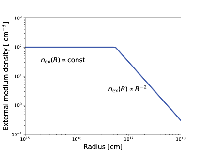
Figure 2: The number density distribution of the external medium as a function of radius from the central engine in the laboratory frame. Here, we adopt $n_{\rm ex,0}=100\rm~{}cm^{-3}$ and $A_{*}=1$.

2.3 Particle acceleration and radiative process

As the relativistic ejecta interact with the external medium, two shocks formed: the forward shock, advancing into the ambient external medium, and the reverse shock, moving backward to decelerate the outflow, as depicted in Fig 1. In this context, we denote the downstream internal energy density (pressure) of the shocked wind medium as $e_{2}$ ($p_{2}$) and the downstream internal energy density (pressure) of the shocked ejecta as $e_{3}$ ($p_{3}$), as depicted in Fig. 1. Given pressure equilibrium across the contact discontinuity, described by $p_{2}=p_{3}$, we find the relation

$$(\hat{\gamma}_{2}-1)e_{2}=(\hat{\gamma}_{3}-1)e_{3},$$ (4)

where $\hat{\gamma}_{2}$ and $\hat{\gamma}_{3}$ represents the adiabatic indices in shocked ejecta and shocked external medium, respectively. The adiabatic indices can be expressed as

$$\hat{\gamma}\approx\frac{4\bar{\gamma}+1}{3\bar{\gamma}},$$ (5)

where $\bar{\gamma}$ represents the average Lorentz factor of particles. For non-relativistic case, $\hat{\gamma}=5/3$, whereas for relativistic case, $\hat{\gamma}=4/3$ (Zhang, 2019).

The amplification of magnetic field strength in the downstream region of the reverse-forward shock system remains unclear (e.g., Medvedev & Loeb, 1999). We parameterize a fraction $\epsilon_{B}$ ($\epsilon_{B}^{r}$) of the downstream internal energy density of the shocked external matter (ejecta) being converted into magnetic field energy density, $u_{B}$ ($u_{B}^{r}$). Both electrons and protons (or ions) can be accelerated as they traverse the shock under the diffusive shock acceleration mechanism (DSA) (e.g., Sironi et al., 2015). These accelerated particles exhibit power-law distributions, with their maximum energy determined by the balance between the acceleration timescale and various energy loss timescales (e.g., Asano et al., 2020). However, the energy content of these nonthermal particles remains unknown. We assume a fraction $\epsilon_{e}$ ($\epsilon_{e}^{r}$) of the downstream internal energy density goes into nonthermal electrons $u_{e}$ ($u_{e}^{r}$), and another fraction $\epsilon_{p}$ ($\epsilon_{p}^{r}$) of the downstream internal energy density is allocated to nonthermal protons $u_{p}$ ($u_{p}^{r}$). These microphysical parameters can potentially be constrained through fitting multi-wavelength afterglow light curves.

Studies have shown that accelerating protons to ultra-high energies (UHE) is a slow process for ultra-relativistic external forward shocks due to the relatively weak magnetic field in the surrounding medium (e.g., Gallant & Achterberg, 1999; Murase et al., 2008; Sironi et al., 2015). Conversely, the reverse shock has been proposed as an alternative acceleration site of for accelerating UHECRs (e.g., Waxman & Bahcall, 2000; Murase, 2007; Murase et al., 2008; Zhang et al., 2018). Unlike the forward shock, the reverse shock is either nonrelativistic or only mildly relativistic (Sari & Piran, 1995; Sari, 1997). Building upon the concept proposed in  Zhang et al. (2023), we explore the acceleration of UHE protons by the reverse shock and investigate proton synchrotron emission while considering the dynamical evolution of the reverse shock.

2.4 Numerical methods

The calculations in this work are based on the Astrophysical Multimessenger Emission Simulator (AMES) code, which is used for numerical modeling of the emission from GRB afterglow. For a comprehensive understanding of the dynamic evolution of the reverse-forward shock system and the associated radiative processes, please refer to Appendix A. In below, we describe the general calculation processes.

The observed flux at a given observation time $T$ could be determined by integrating over the equal-arrival-time-surface (EATS) (e.g., Zhang, 2018). In our calculations, we adopt the thin-shell limit (van Eerten et al., 2010; Ryan et al., 2020; Takahashi & Ioka, 2020; Takahashi et al., 2022). The observed flux can be estimated as follows (e.g. Takahashi et al., 2022)

$$F_{E}(T) =\frac{1}{d_{L}^{2}}\int_{0}^{\theta_{j}}d\theta{\rm sin}\theta\int_{0}^{2\pi}d\phi\frac{R^{2}|\mu-\beta_{\rm sh}|}{1-\mu\beta_{\rm sh}}$$

$$\times\frac{j_{E}}{\alpha_{E}}(1-e^{-\tau_{E}})|_{t=T+\mu R/c}.$$ (6)

Here, $T$ represents the observation time, $d_{L}$ stands for the luminosity distance of the source, $\theta$ denotes the polar angle measured from the jet axis, $\phi$ represents the azimuth angle, and $t$ represents the laboratory time. Note we neglect the redshift dependence. The term $\mu$ is given by

$$\mu={\rm sin}\theta{\rm sin}\theta_{v}{\rm cos}\phi+{\rm cos}\theta{\rm cos}\theta_{v},$$ (7)

which defines the cosine of the angle formed by the radial vector and the line-of-sight. Here, $\theta_{v}$ corresponds to the viewing angle measured from the jet axis. The shock velocity, denoted as $\beta_{\rm sh}=\sqrt{1-\Gamma_{\rm sh}^{-2}}$, where $\Gamma_{\rm sh}=\sqrt{2}\Gamma$, with $\Gamma$ represents the Lorentz factor of the blast wave. In our calculations, we set $T=0$ as the arrival time when a photon is emitted at the origin at the laboratory time $t=0$. The width of the shocked shell in the laboratory frame is given by

$$w=\frac{R}{12\Gamma^{2}}.$$ (8)

We define $\Delta s$ as the length along a ray travel the shocked region where emitted photons reach the observer at time $T$. In the general case, considering absorption, the value of $\Delta s$ can be expressed as

$$\Delta s=\frac{R}{12\Gamma^{2}|\mu-\beta_{\rm sh}|},$$ (9)

as shown in Takahashi et al. (2022). In the optically thin limit, Eq. 2.4 can be simplified as

$$F_{E}(T) =\frac{1}{d_{L}^{2}}\int_{0}^{\theta_{j}}d\theta{\rm sin}\theta\int_{0}^{2\pi}d\phi R^{2}\Delta Rj_{E}|_{t=T+\mu R/c},$$ (10)

where

$$\Delta R=\frac{R}{12\Gamma^{2}(1-\mu\beta_{\rm sh})}$$ (11)

represents the radial integration path that contributes to the observed flux at a given observation time $T$.

The emissivity measured in the laboratory frame is

$$j_{E}=\frac{j_{\varepsilon}}{\Gamma^{2}(1-\beta\mu)^{2}},$$ (12)

where $j_{\varepsilon}$ is the comoving frame emissivity per unit volume per second per solid angle, and

$$E=\delta\varepsilon=\frac{\varepsilon}{\Gamma(1-\beta\mu)},$$ (13)

is the observed photon energy in the laboratory frame and $\delta$ is the Doppler factor. The absorption coefficient in the laboratory frame is given by

$$\alpha_{E}=\Gamma(1-\beta\mu)\alpha_{\varepsilon},$$ (14)

where $\alpha_{\varepsilon}$ is measured absorption coefficient in the comoving frame. The corresponding opacity can be derived via integration over the line of sight,

$$\tau_{E}=\int\alpha_{E}ds\approx\alpha_{E}\Delta s.$$ (15)

In this work, we primarily focus on two key attenuation processes: the synchrotron self-absorption (SSA), crucial for understanding low-frequency radio emission, and $\gamma\gamma$ pair production, which affects the escape of VHE gamma-rays. In the latter situation, the primary targets for interaction are the nearby low-energy synchrotron photons emitted by nonthermal electrons. The absorption coefficient is estimated as

$$\alpha_{\varepsilon}\approx\frac{1}{ct_{\gamma\gamma}},$$ (16)

where $t_{\gamma\gamma}$ is the comoving frame interaction timescale. During our numerical calculation process, we initially overlook the $\gamma\gamma$ attenuation caused by prompt photons. However, we later account for this effect in a subsequent post-processing step, which we detail in the next section. Note in our calculations, we perform calculations in the momentum space, where the Deep Newtonian limit is avoided (Huang & Cheng, 2003; Sironi & Giannios, 2013; Wei et al., 2023; Ryan et al., 2023).

3 VHE gamma-rays from GRB afterglow

3.1 Early afterglow in the VHE band

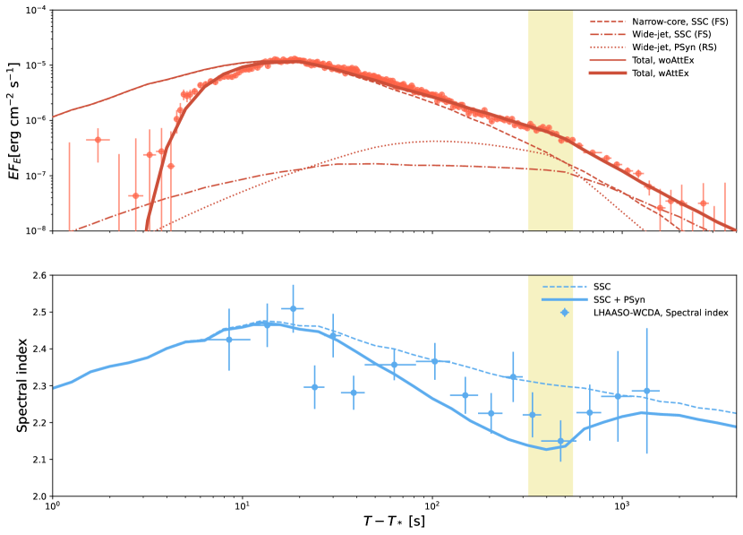
Figure 3: Predicted energy flux (upper panel) and spectral index (lower panel) evolution in the VHE band within the two-component structured jet model. The yellow band indicates the region where there is a small flare.

In the upper panel of Fig. 3, we compare numerical results with energy flux measurements by LHAASO-WCDA integrated over the 0.3 TeV to 5 TeV energy range (Cao et al., 2023b), where the corresponding parameters are listed in Table 1. There’s a clear agreement between the predicted light curve (solid red line) and the measured energy flux (red dots) for about $T-T_{*}\sim 3000$ seconds after the GBM trigger, where $T_{*}$ is the reference time at the onset of the main component (Cao et al., 2023b).

However, our model’s light curve shows an inconsistency with the measured one at early times, $T-T_{*}\lesssim 10\rm~{}s$, see solid thin lines. To be specific, the LHAASO-WCDA light curve exhibits an initial rapid rise with a power-law index of approximately $14.9$, followed by a slower ascent with a power-law index of roughly $1.82$, leading up to its peak value (Cao et al., 2023b). In contrast, our predicted early light curve is less steep than the observed value, see solid red line. One potential explanation for this discrepancy could be the rapid initial rise being influenced by $\gamma\gamma$ attenuation due to the intense prompt photons (e.g., Zhang et al., 2023; Khangulyan et al., 2023a). Note a different $T_{*}$ will give a different rising slope, which could change above interpretation.

The number density of the prompt photons at the external shocked region can be estimated as

$$u_{\rm GRB\gamma}\approx L_{\rm GRB\gamma}^{\rm iso}/4\pi R^{2}\Gamma^{2}c,$$ (17)

where $L_{\rm GRB\gamma}^{\rm iso}$ represents the isotropic-equivalent gamma-ray luminosity. The optical depth can be approximated as follows:

$$\tau_{\gamma\gamma}^{\rm prompt}\simeq 220\frac{\eta_{\gamma\gamma,-1}L_{\rm GRB\gamma,53.5}^{\rm iso}}{R_{16}\Gamma_{2}^{2}E_{\rm pk,\rm MeV}}\begin{cases}(E_{\gamma}/\tilde{E}_{\gamma,b})^{\beta-1},E_{\gamma}<\tilde{E}_{\gamma,b}\\ (E_{\gamma}/\tilde{E}_{\gamma,b})^{\alpha-1},E_{\gamma}>\tilde{E}_{\gamma,b}\end{cases}.$$ (18)

Here, $\alpha$ and $\beta$ represent the spectral indices of the prompt emission, and $\tilde{E}_{\gamma,b}\approx\Gamma_{\times}^{2}m_{e}^{2}c^{4}/E_{\rm pk,\rm MeV}\simeq 2.6~{}\Gamma_{\times,2}^{2}\rm~{}GeV$ denotes the typical energy of high-energy $\gamma$-rays that interact with target photons of peak energy $E_{\rm pk,MeV}$ in the observer frame (Zhang et al., 2023). Please note that we are disregarding the anisotropic scattering effect of the beamed prompt photons. During the early phase, the jet is in the coasting state with a Lorentz factor of approximately $\Gamma\approx\Gamma_{0}$, and the radius of the external shock is approximately $R\approx 2\Gamma_{0}^{2}c(T-T_{*})$. For illustrative purposes, we’ve parameterized the time evolution of the optical depth as

$$\tau_{\gamma\gamma}^{\rm prompt}=\tau_{\gamma\gamma,0}\left(\frac{T-T_{*}}{1\rm~{}s}\right)^{-s_{\tau}},$$ (19)

where $\tau_{\gamma\gamma,0}=180$ and $s_{\tau}=3$. In this context, we assume that $L_{\rm GRB\gamma}^{\rm iso}\propto(T-T_{*})^{-2}$ and that $R\propto(T-T_{*})$ during the early afterglow phase. The prompt emission flux in the 20 keV - 10 MeV range is $1.62\times 10^{-2}\rm~{}erg~{}cm^{-2}~{}s^{-1}$ during the time interval $T_{0}+[225.024-233.216]\rm~{}s$ and $3.15\times 10^{-4}\rm~{}erg~{}cm^{-2}~{}s^{-1}$ during the time interval $T_{0}+[241.408-249.600]\rm~{}s$ (Frederiks et al., 2023). The energy flux decreases by two orders of magnitude when the VHE gamma-ray light curve reaches its peak. The observed flux in the VHE band, after accounting for the $\gamma\gamma$ attenuation by the prompt photons, can be obtained as,

$$EF_{E}(T-T_{*})=EF_{E}(T-T_{*})|_{\rm woAttEx}\ {\rm exp}\left[-\tau_{\gamma\gamma}^{\rm prompt}(T-T_{*})\right],$$ (20)

where $EF_{E}(T-T_{*})|_{\rm woAttEx}$ is the flux without considering the attenuation by external prompt photons. Therefore, we attribute the rapid increase in early TeV afterglow data to the effect of $\gamma\gamma$ attenuation by the prompt photons, which aligns with the argument presented in (Khangulyan et al., 2023a; Shen et al., 2023).

The energy flux in the VHE band peaks around $T-T_{*}\sim 18\rm~{}s$, which is consistent with the jet’s duration, approximately $\delta T_{\rm ej}\sim 10\rm~{}s$. Following the peak, the energy flux decreases over time, displaying a power-law spectral index of about $1.1$, consistent with the findings reported by Cao et al. (2023b). It was also noted in Cao et al. (2023b) that the sharp decline in flux around $T-T_{*}\sim 670~{}\rm~{}s$ aligns with the jet break, resulting in an energy flux decreases with a power-law index of approximately $2.2$. In our study, we propose an alternative explanation. We suggest that the steep drop in the light curve is caused by the emission from the wide jet (depicted as a red dotted-dash curve), while the jet break in the emission from the narrow core occurred earlier. Furthermore, there’s a small flare around $T-T_{*}=[320,550]\rm~{}s$ as reported in (Cao et al., 2023b). In our model, the emergence of reverse shock proton synchrotron emission (illustrated as a red dotted curve) appears to coincide with this observed flare.

Table 1: Physical parameters adopted in this work.

[b] Parameter Narrow-core Wide-Jet $\mathcal{E}_{k}[\rm erg]$ $4\times 10^{55}$ $4\times 10^{55}$ $\Gamma_{0}$ $430$ $400$ $n_{\rm ex,0}[\rm cm^{-3}]$ $100$ $100$ $A_{*}$ 1 1 $k$ 2 2 $\delta T_{\rm ej}[\rm s]$ $10$ $400(3000)$¹ $\theta_{j}$ [deg] 0.22 5.7 $\theta_{c}[\rm rad]$ - 0.03 $a$ - 2 $\theta_{v}[\rm deg]$ 0 0 $\epsilon_{B}$ $2\times 10^{-4}$ $2\times 10^{-4}$ $\epsilon_{e}$ $1.1\times 10^{-2}$ 0.005 $f_{e}$ $0.3$ 0.015 $s_{e}$ $2.3$ $2.3$ $\epsilon_{B}^{r}$ - $0.3$ ($0.1$)² $\epsilon_{e}^{r}$ - $0.002$ $f_{e}^{r}$ - $0.008$ $s_{e}^{r}$ - $2.4$ $\epsilon_{p}^{r}$ - $0.6$ $s_{p}^{r}$ - $2$

• $\delta T_{\rm ej}=3000\rm~{}s$ when $\theta_{j}>1.1$ deg.

• $\epsilon_{B}=0.1$ when $\theta_{j}>1.1$ deg.

3.2 Spectral hardening and reverse shock proton synchrotron emission

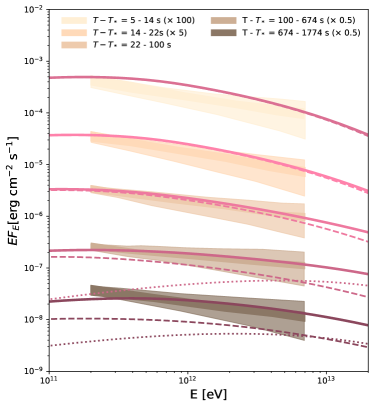
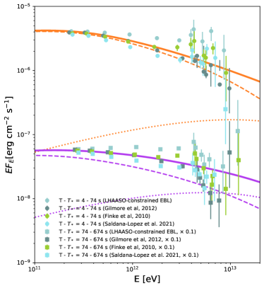
Figure 4: The expected VHE gamma-ray energy spectrum from GRB 221009A during the afterglow phase. The dashed lines depict SSC radiation from the forward shock of the narrow core, while dotted lines show proton synchrotron emission from the reverse shock of the wide jet. In the left panel, we compare our theoretical model with the measured energy spectra from LHAASO-WCDA, which go up to 7 TeV. The measurements have been adjusted using an EBL model (Saldana-Lopez et al., 2021; Cao et al., 2023b). The inner bands represent statistical uncertainties, and the outer bands indicate systematic uncertainties. In the right panel, we compare the intrinsic energy spectra after correction for various EBL models, including data from LHAASO-KM2A (Cao et al., 2023a).

In the lower part of Fig. 3, we compare the predicted spectral index evolution with the observed data, where the spectral index is defined as $EF_{E}=E^{-s+2}$. We notice a subtle trend in the spectral index as time progresses (Cao et al., 2023b). Initially, during the rising phase at $T-T_{*}\sim 10-20\rm~{}s$, it’s relatively soft at around $2.4$. As the time elapses, it gradually decreases, reaching a minimum spectral index of approximately $2.2$ at $T-T_{*}\sim 400\rm~{}s$. Afterward, it starts to become softer again, with a spectral index of around $\sim 2.3$ at $T-T_{*}\sim 1000\rm~{}s$. We observed that the spectral index evolution of the SSC component from the narrow jet does not match the measured values where the spectral index gradually decreases from $2.4$ to $2.3$, as shown by the dashed curve. Remarkably, the observed change in spectral index finds a straightforward explanation with the introduction of an additional component: the reverse shock proton synchrotron emission. The energy spectral index of this proton synchrotron emission is $(s_{p}^{r}+1)/2=3/2$ for $s_{p}^{r}=2$, which is significantly harder compared to the inverse-Compton spectral index in the TeV energy range (e.g., Zhang et al., 2023). We notice that the spectral index’s shift towards harder values aligns well with the peak time of the proton synchrotron emission. Furthermore, this change in spectral behavior correlates with the emergence of a flare at $T-T_{*}=[320,550]\rm~{}s$ (Cao et al., 2023b).

In Fig. 4, we show the calculated energy spectrum in the early phase ($T-T_{*}<2000\rm~{}s$) of the VHE band, taking into account $\gamma\gamma$ attenuation by prompt photons as in Eq. 20. What we see is that the primary source of the observed flux is the SSC emission from the narrow core. Furthermore, the later spectral hardening observed can be attributed to the reverse shock proton synchrotron emission from the wide jet.

Next, we’ll analytically estimate the proton synchrotron emission from the reverse shock at the time of shock crossing, referred to as $T_{\times}$. To do this, we assume that the duration of the GRB ejecta, measured in the stellar frame, is $\delta T_{\rm ej}=100\rm~{}s$. The width of the ejecta, measured in the stellar frame, can be approximated as:

$$\Delta_{0}\approx c\delta T_{\rm ej}\simeq 3\times 10^{12}\delta T_{\rm ej,2}\rm~{}cm.$$ (21)

We can estimate the jet spreading radius as:

$$\Delta_{s}=R_{\rm dec}/2\Gamma_{0}^{2}\simeq 2.8\times 10^{11}\mathcal{E}_{54.5}^{1/3}\Gamma_{0,2.5}^{-8/3}n_{\rm ex,2}^{-1/3}\rm~{}cm.$$ (22)

Given the condition $\Delta_{0}>\Delta_{s}$, the jet spreading effect is not significant. The radius at which the reverse shock crosses is approximately,

$$R_{\times}\simeq 6.4\times 10^{16}\mathcal{E}_{54.5}^{1/4}\delta T_{\rm ej,2}^{1/4}n_{\rm ex,2}^{-1/4}\rm~{}cm.$$ (23)

At the time $T_{\times}=\delta T_{\rm ej}$, the Lorentz factor of the shocked ejecta is

$$\Gamma_{\times}\simeq 86\mathcal{E}_{54.5}^{1/8}\delta T_{\rm ej,2}^{-3/8}n_{\rm ex,2}^{-1/8}.$$ (24)

The relative Lorentz factor of the shocked ejecta, when measured in the unshocked ejecta frame, is

$$\Gamma_{34}\simeq 1.9.$$ (25)

The number density of the unshocked ejecta in the comoving frame can be calculated as

$$n_{\rm ej} =\frac{\mathcal{E}_{k}}{4\pi m_{p}c^{2}\Gamma_{0}(\Gamma_{0}\Delta_{0})R_{\times}^{2}}$$

$$=2.5\times 10^{5}\mathcal{E}_{54.5}^{1/2}\Gamma_{0,2.5}^{-2}\delta T_{\rm ej,2}^{-3/2}n_{\rm ex,2}^{1/2}\rm~{}cm^{-3}.$$ (26)

The magnetic field strength can be determined as follows,

$$B_{\times} =(32\pi\epsilon_{B}^{r}\Gamma_{34}n_{\rm ej}(\Gamma_{34}-1)m_{p}c^{2})^{1/2}$$

$$\simeq 135\epsilon_{B,-0.5}^{r1/2}\mathcal{E}_{54.5}^{1/4}\Gamma_{0,2.5}^{-1}\delta T_{\rm ej,2}^{-3/4}n_{\rm ex,2}^{1/4}(g(\Gamma_{34})/2.4)^{1/2}\rm~{}G,$$ (27)

where $g(\Gamma_{34})\equiv(\Gamma_{34}-1)(\Gamma_{34}+3/4)$. The maximum proton energy under the confinement condition $t_{\rm acc}<t_{\rm dyn}$ can be estimated as,

$$E_{p,\rm max}^{\rm dyn} \approx\eta^{-1}eB_{\times}R_{\times}$$

$$\simeq 2.7\times 10^{21}\eta^{-1}\epsilon_{B,-0.5}^{r\frac{1}{2}}\mathcal{E}_{54.5}^{\frac{1}{2}}\Gamma_{0,2.5}^{-1}\delta T_{\rm ej,2}^{\frac{-1}{2}}\left(\frac{g(\Gamma_{34})}{2.4}\right)^{\frac{1}{2}}~{}{\rm~{}eV},$$ (28)

where $\eta$ is a coefficient which is a few in the Bohm limit  (e.g., Sironi et al., 2015). The maximum energy is limited by the synchrotron cooling process, and we find,

$$E_{p,\rm max}^{\rm syn} =\sqrt{\frac{6\pi e}{\sigma_{T}B_{\times}\eta Z^{3}}}\frac{m_{p}^{2}c^{2}}{m_{e}}\Gamma_{\times}$$

$$\simeq 1.4\times 10^{21}\eta^{\frac{-1}{2}}Z^{\frac{-3}{2}}\epsilon_{B,-0.5}^{r\frac{-1}{4}}\Gamma_{0,2.5}^{\frac{-1}{2}}n_{\rm ex,2}^{\frac{-1}{4}}\left(\frac{g(\Gamma_{34})}{2.4}\right)^{\frac{-1}{4}}\rm~{}eV.$$ (29)

The maximum energy of protons is then given by

$$E_{p,\rm max}={\rm min}[E_{\rm max}^{\rm dyn},E_{\rm max}^{\rm syn}].$$ (30)

The flux of the synchrotron emission, which peaks at the maximum energy $\varepsilon_{\gamma}={\rm min}[\varepsilon_{\gamma,M},\varepsilon_{\gamma,c}]$, can be expressed as

$$F_{E}=\frac{1+z}{4\pi d_{L}^{2}}N_{3}(E_{p,\rm max})P_{E},$$ (31)

Here, $N_{3}(E_{\rm max})$ represents the number of protons, and $P_{E}$ is the laboratory frame specific synchrotron power per proton,

$$P_{E} \approx\frac{\phi_{0}\sqrt{3}e^{3}}{m_{p}c^{2}}B_{\times}\Gamma_{\times}$$

$$\simeq 1.5\times 10^{-21}\rm~{}erg~{}s^{-1}~{}Hz^{-1},$$ (32)

where $\phi_{0}$ is a factor of order unity. The typical frequency of the proton synchrotron emission in the observer frame is given by

$$E_{\rm max} \approx\frac{3}{4\pi}\frac{heB_{\times}}{m_{p}c}\gamma_{p,\rm max}^{2}\Gamma_{\times}/(1+z)$$

$$\simeq 3.5\times 10^{13}/(1+z)\rm~{}eV,$$ (33)

where $\gamma_{p,\rm max}=(E_{p,\rm max}/\Gamma_{\times})/m_{p}c^{2}$ is the maximum Lorentz factor of protons.

The comoving frame energy density of non-thermal protons can be calculated as

$$\int_{\varepsilon_{p,\rm min}}^{\varepsilon_{p,\rm max}}d\varepsilon_{p}\varepsilon_{p}\frac{dn}{d\varepsilon_{p}}=\epsilon_{p}^{r}e_{3}=4\epsilon_{p}^{r}\Gamma_{34}(\Gamma_{34}-1)n_{\rm ej}m_{p}c^{2}.$$ (34)

The total number density of non-thermal protons is given by

$$n_{p,3}=\int_{\varepsilon_{p,\rm min}}^{\varepsilon_{p,\rm max}}d\varepsilon_{p}\frac{dn}{d\varepsilon_{p}}.$$ (35)

The number of protons at $E_{p,\rm max}$ can be estimated as

$$N_{3}(E_{p,\rm max}) \approx 4\pi R_{\times}^{2}\Delta_{\times}\varepsilon_{p}\frac{dn}{d\varepsilon_{p}}|_{\varepsilon_{p}=\varepsilon_{p,\rm max}}$$

$$\approx 4\pi R_{\times}^{2}\Delta_{\times}\frac{\epsilon_{p}^{r}4\Gamma_{34}(\Gamma_{34}-1)n_{\rm ej}m_{p}c^{2}}{\rm{ln}(\varepsilon_{p,\rm max}/\varepsilon_{p,\rm min})\varepsilon_{p,\rm max}}$$

$$\simeq 1.5\times 10^{43},$$ (36)

assuming $s_{p}^{r}=2$. Finally, we can derive the differential flux estimated at $E_{\rm max}$ as

$$EF_{E}|_{E=E_{\rm max}}\simeq 3.2\times 10^{-6}\rm~{}erg~{}cm^{-2}~{}s^{-1}.$$ (37)

We can see the estimated flux is consistent with Fig. 3 and Fig. 4.

3.3 Late-time afterglow and reverse shock emission

In Fig. 5, we compare the predicted multi-wavelength light curve with the observed flux across a wide range of energy bands, from radio to VHE.

Early on, roughly within the first $10^{3}\rm~{}s$, the energy flux is mainly attributed to the external forward shock emission from the narrow jet. However, at later times, beyond approximately $10^{3}-10^{4}\rm~{}s$, the dominant contribution to the energy flux shifts to the external forward shock emission from the wide jet. This transition is highlighted in the left panel of Fig. 5.

In the right panel, we further analyze the energy flux evolution in the lower energy range compared to the observed flux, spanning from radio to optical bands. Around $T-T_{*}=10^{4}\rm~{}s$, the energy flux in the optical bands is primarily governed by the external forward shock synchrotron emission from the wide jet. However, in the radio band, the external forward shock synchrotron emission from the narrow core dominates the energy flux until around $T-T_{*}=10^{4}\rm~{}s$, when the wide jet’s emission takes over.

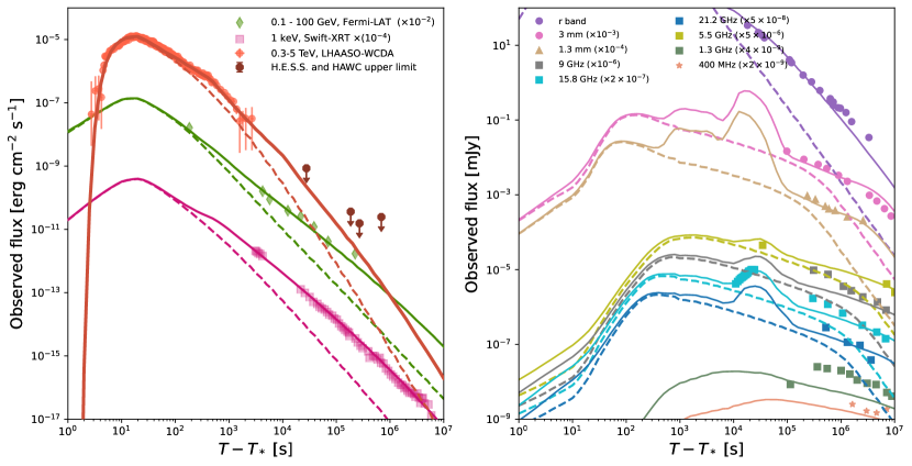
Figure 5: Predicted afterglow light curve for GRB 221009A across multiple wavelengths. The solid lines represent the combined emission from both the narrow core and wide jet, while the dashed lines depict the contributions from the narrow core alone. Light curves for radio, millimeter, optical and X-ray are taken from (Laskar et al., 2023; O’Connor et al., 2023; Bright et al., 2023). The optical data is corrected for extinction. The Fermi-LAT light curve is obtained from (Bissaldi et al., 2023), and the TeV light curve is obtained from (Cao et al., 2023b). Upper limits in the VHE band from H.E.S.S. and HAWC are taken from (Mbarubucyeye et al., 2023).

In Fig. 6, we compare the reverse shock electron synchrotron emission from the wide jet to the observed data in the low-energy radio to optical bands. Although it’s not as prominent as the forward shock emission, unlike the reverse shock emission, the forward shock light curve is expected to remain relatively constant in the case of a wind medium, which aligns with the findings presented in  Gill & Granot (2023). They considered emission from a shallow angular structured jet similar to our wide jet component in the thick shell scenario (Gill & Granot, 2023). Similar to  Gill & Granot (2023); Zheng et al. (2023); Ren et al. (2023a), we found that the reverse shock emission from the wide jet is considerably higher than the forward shock emission at $T\sim 10^{4}\rm~{}s$ which could account for the observed bump at $\sim 10-20\rm~{}GHz$ (Bright et al., 2023; Gill & Granot, 2023; Zheng et al., 2023; Ren et al., 2023a). Note the two bumps on the reverse shock emission is related to the duration of the ejecta, which is $T_{\rm ej}=300\rm~{}s$ for $\theta<1.1^{\circ}$ and $T_{\rm ej}=3000\rm~{}s$ for $\theta>1.1^{\circ}$. It’s important to note that photons from the reverse shock electron synchrotron emission play a significant role as they can impact the escape of VHE photons above 10 TeV, which are generated through proton synchrotron emission.

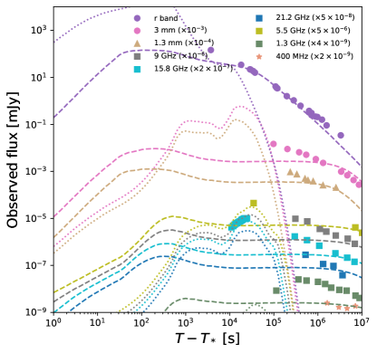
Figure 6: Similar to Fig. 5, we compare the reverse-forward shock emission from the wide jet to the observed data in the low-energy radio to optical bands. The dashed lines represent the external forward shock emission, while the dotted lines represent the external reverse shock emission.

4 Discussion and implications

4.1 VHE gamma-rays from GRBs

In our analysis, we thoroughly investigate the two primary sources of VHE gamma-rays in GRB 221009A: SSC emission and proton synchrotron emission. Here’s what we found:

• For the SSC process, our calculations reveal that narrow-core SSC emission dominates the early TeV afterglow, while the wide-jet SSC emission takes over in the later stages.

• Proton synchrotron emission becomes most significant during the transition phase around $T-T_{0}\sim 600\rm~{}s$, where the reverse shock finishes crossing the ejecta of the wide jet. Although the proton synchrotron component doesn’t dominate the entire VHE band light curve, it plays a crucial role during this critical period.

A closer examination of the VHE spectral index reveals an intriguing pattern: the VHE spectra start soft, then become hard, and finally steepen in the late stages. This evolution trend is challenging to explain within the standard SSC model alone. It seems more natural to introduce an additional component responsible for spectral hardening. The proton synchrotron component offers a plausible explanation because it inherently produces harder spectral indices. Note the similar behavior of spectral hardening at late time has also been observed in GRB 190829A, which is difficult to explain within the standard SSC model (Abdalla et al., 2019). The reverse shock proton synchrotron component discussed in this work could be helpful to alleviate the limitation of the standard SSC model.

Given pressure balance, we can approximate $e_{2}\sim e_{3}$. Assuming that the micro-physical parameter $\epsilon_{B}^{r}$ is much larger than $\epsilon_{B}$, we deduce that $u_{B}^{r}\gg u_{B}$. This implies that the magnetic field strength is significantly stronger in the shocked ejecta region than in the shocked external matter region. Consequently, our focus is primarily on proton synchrotron emission in the shocked ejecta region. It is possible that the magnetic field strength is significantly amplified, and the micro-physical parameter $\epsilon_{B}$ could be much higher than the value adopted in this work, even in the case of the forward shock. Under such circumstances, and assuming that proton can be accelerated to UHE, proton synchrotron emission might explain the observed TeV flux from GRB, where the electron inverse Compton process being of lesser importance, as discussed in Isravel et al. (2023a). However, the fitting to the lightcurve performed in  Isravel et al. (2023a) neglects the constrains made by the late time radio to millimeter band data. Additionally, Isravel et al. (2023a) could not explain the shape of the TeV lightcurve measured by LHAASO. In any case, further investigation is required to determine whether proton synchrotron emission can account for the observed evolution of the energy spectral index observed by LHAASO in the VHE band.

In this work, we employ a two-component jet model to explain the VHE gamma-rays observed by LHAASO. As demonstrated in Section 3.3, the wide-jet component is necessary to account for the late-time radio to optical data. Specifically, the reverse shock radio emission from the wide-jet component aligns with the observed optically thick rising radio light curve.

The model parameters we found for the wide-jet component are very similar to those adopted in  Gill & Granot (2023). For example, the isotropic equivalent kinetic energy $\mathcal{E}_{k}$, $A*$, and $\epsilon_{B}$ are around 2 times larger than those in  Gill & Granot (2023). Our value of $\epsilon_{e}$ is 2 times smaller. The power-law index of the energy angular profile $a=2$ is larger than the value $a\sim 0.8$ found in  Gill & Granot (2023). However, Gill & Granot (2023) only conducted fitting to the late-time radio to X-ray band, aligning with our results. Based on Fig.3, we found that the SSC emission from the wide-jet (dotted-dashed line) cannot explain the TeV light curve, contributing significantly only at late time $T-T_{0}\sim 1000$ seconds. Thus, the observed TeV light curve needs to be explained with another jet component, e.g., the narrow-core (e.g., Cao et al., 2023b). In comparison to the model parameters adopted in  Cao et al. (2023b), the width of the narrow core is slightly narrower, with $\theta_{j}\sim 0.22$ degrees. This narrower jet is necessary to avoid overshooting the late-time radio data. Our calculations suggest that the change in the decaying slope of the light curve is attributed to the emergence of the wide-jet component.

Both works from Zheng et al. (2023) and Ren et al. (2023a) performed multiwavelength fitting up to the TeV band for GRB 221009A, considering a two-component structured jet model. However, both the model details and the values of physical parameters differ. The isotropic equivalent energy of the wide-jet component we found is over $\sim 1$ order of magnitude more energetic than  Zheng et al. (2023), but consistent with Ren et al. (2023a). Compared to  Zheng et al. (2023) and  Ren et al. (2023a), our model is more consistent with the light curve at $100\rm~{}GHz$ band. We found that the observed X-ray flux around 3000 seconds is dominated by the wide-jet component, which is underpredicted in  Ren et al. (2023a). Finally, we should note that our model involves the reverse shock proton synchrotron emission in addition to the SSC component, providing a better description of the TeV light curve and energy spectrum measured by LHAASO.

4.2 High-energy neutrinos from GRBs

In this section, we present the expected flux of high-energy neutrinos from the reverse shock proton synchrotron model. The GRB afterglow is expected to emit PeV-EeV neutrinos via photomeson production process (Waxman & Bahcall, 2000; Dermer, 2002; Li et al., 2002; Murase, 2007; Razzaque, 2013). However, there are no evidence of correlation between neutrinos and GRBs analysed with candidated muon-neutrino events observed by IceCube  (Abbasi et al., 2022; Lucarelli et al., 2023). Abbasi et al. (2022) found the total contributions to the quasi-diffuse neutrino flux is less than $24\%$ for an emission timescale $10^{4}$ seconds. The detection of PeV-EeV neutrinos would require future UHE neutrino telescopes such as GRAND 200k (Álvarez-Muñiz et al., 2020), IceCube-Gen2 (Abbasi et al., 2021), RNO-G (Aguilar et al., 2021), as well as POEMMA (Venters et al., 2020).

The neutrino fluence could be approximated as (e.g., Murase et al., 2022; Kimura, 2022)

$$E_{\nu}^{2}\phi_{\nu_{\mu}} \approx\frac{1}{8}\frac{1+z}{4\pi d_{L}^{2}}{\rm min}[1,f_{p\gamma}]f_{\pi,\rm sup}f_{\mu,\rm sup}\mathcal{E}_{\rm cr}\frac{1}{\mathcal{R}_{\rm cr}}$$

$$\simeq 4.9\times 10^{-2}{\rm min}[1,f_{p\gamma}]f_{\pi,\rm sup}f_{\mu,\rm sup}\rm~{}GeV~{}cm^{-2},$$ (38)

where $f_{p\gamma}$ is the effective optical depth of photomeson production process, $f_{\pi,\rm sup}$ is the suppression factor by pion cooling, $f_{\mu,\rm sup}$ is the suppression factor by muon cooling,

$$\mathcal{E}_{\rm cr}=\epsilon_{p}^{r}4\pi R_{\times}^{2}\Delta_{\times}e_{3}\Gamma_{\times}\simeq 7.6\times 10^{53}\rm~{}erg.$$ (39)

is the isotropic-equivalent cosmic ray proton energy accelerated by reverse shock, and

$$\mathcal{R}_{\rm cr}=\rm{ln}(\varepsilon_{p,\rm max}/\varepsilon_{p,\rm min})\simeq 23.$$ (40)

converts the bolometric cosmic ray energy to the differential cosmic ray energy. In Fig. 7, we show the predicted single flavor neutrino fluence in the reverse shock proton synchrotron model, which are numerically calculated with Eq. 2.4 by integrating over the EATS. At the peak energy, the corresponding photomeson production efficiency is estimated to be $f_{p\gamma}\lesssim 0.1$ at the shock crossing time. For comparison purpose, we also present the neutrino fluence expected in the forward shock model, assuming a fraction of $\epsilon_{p}=0.1$ of the post-shock thermal energy goes into high-energy protons and protons could be accelerated to ultra-high-energy. The accelerated protons following powerlaw distribution with spectral index $s_{p}=2$. We can see that the predicted neutrino fluence peaked at ultra-high-energy range and is lower than the 90% C.L. upper limits by IceCube. Even though the neutrino flux from single GRB is undetectable, the diffuse neutrino flux contributed from all GRBs could provide valuble tests of the model.

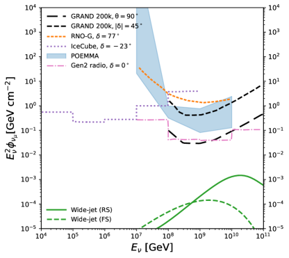
Figure 7: Neutrino fluence predicted in the reverse shock proton synchrotron model for both narrow-core and wide-jet. For comparison purpose, we also present the neutrino fluence expected in the forward shock model, assuming a fraction of $\epsilon_{p}=0.1$ of the post-shock thermal energy goes into high-energy protons. We show the sensitivity of GRAND for a source at declination $\delta=45^{\circ}$ and zenith angle $\theta=90^{\circ}$ (Álvarez-Muñiz et al., 2020), RNO-G at $\delta=77^{\circ}$ (Aguilar et al., 2021), IceCube-Gen2 radio at $\delta=0^{\circ}$ (Abbasi et al., 2021), IceCube at $\delta=-23^{\circ}$ (Abbasi et al., 2021), and POEMMA taking the 90% unified confidence level and assuming observations during astronomical night (Venters et al., 2020).

4.3 GRBs as UHECR sources

In this study, we examined proton synchrotron emission from protons accelerated to ultra-high energies. We estimated that the total energy of these accelerated non-thermal protons is approximately $\mathcal{E}_{\rm cr}\sim 10^{54}\rm~{}erg$. However, detecting escaping UHECR protons from GRBs simultaneously with VHE gamma-rays is challenging. UHECR undergoes various energy loss processes during the journey to Earth (e.g., Waxman, 1995; Vietri, 1996). The influence of magnetic fields within both host galaxies and extragalactic space can not be neglected. These magnetic fields can introduce significant time delays in the arrival of UHECRs compared to the rectilinear propagation scenario (e.g., Miralda-Escudé & Waxman, 1996; Murase & Takami, 2009). Note the magnetic field in our galaxy also deflects the arrival direction of UHECRs and causes time delay. It has been shown that the UHECR-induced intergalactic electromagnetic cascades might contribute to observed VHE gamma-rays (Alves Batista, 2022; Das & Razzaque, 2023; Mirabal, 2022). However, the time delay and the development of the electromagnetic cascades strongly depend on the structure and strength of intergalactic magnetic fields, which require further investigation.

5 Summary

In this study, we conducted a comprehensive investigation of radiation within the standard external reverse-forward shock scenario, considering a two-component structured jet comprising a narrow core dominated by magnetic energy and a wide jet dominated by matter. We compared our numerical findings with observed energy spectra and multi-wavelength light curves spanning from radio to VHE bands. Our key results are summarized as follows:

• The energy flux light curve observed in the VHE band is primarily dominated by SSC emission from the narrow core. The SSC emission from the wide jet only becomes dominant at late times, approximately beyond $10^{3}$ seconds. Reverse shock proton synchrotron emission becomes significant when the reverse shock crosses the shocked ejecta of the wide jet around $T-T_{0}\sim 600$ seconds, coinciding with the emergence of a mild flare around $T-T_{0}\sim[546,776]$ seconds after the trigger.

• The initial rapid rise of the VHE band light curve is due to $\gamma\gamma$ attenuation caused by prompt target photons, although the reference time $T_{*}$ is uncertain and a different $T_{*}$ changes the early light curve significantly.

• Compared to the inverse-Compton process, reverse shock proton synchrotron emission exhibits a much harder spectrum in the VHE band. This naturally explains the observed energy spectrum hardening and potentially contributes significantly to the photon flux above $\gtrsim 10\rm~{}TeV$.

• The multi-wavelength afterglow lightcurve from radio to the GeV band can be explained within the two-component structured jet model. The emission from the wide jet starts to dominate the observed multi-wavelength afterglow after $T-T_{0}\sim 10^{3}-10^{4}$ seconds, while radio emission from the narrow core may continue to dominate the flux at even later times, until around $T-T_{0}\sim 10^{4}$ seconds. The reverse shock emission from the wide jet from could explain the steep rising of the $\sim 10\rm~{}GHz$ radio data at $T-T_{0}\sim 10^{4}$ seconds.

• Our findings may support the idea that GRBs are efficient accelerators of UHECRs, especially at the reverse shock. Further multimessenger observations involving more events are essential to better understand the energy budget of UHECRs originating from GRBs.

Data Availability

The data developed for the calculation in this work is available upon request.

Appendix A Numerical modeling of the radiation from the external reverse-forward shock

A.1 Dynamics

When the ultra-relativistic ejecta of the GRB propagates into the external medium, the ejecta is decelerated as its kinetic energy is transferred to the external medium. Two shocks are formed: one is the forward shock advancing into the ambient external medium, and the other is the reverse shock moving backward to decelerate the outflow, as illustrated in Fig. 8.

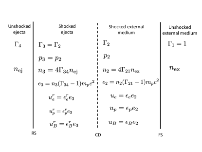
Figure 8: Radiation from reverse-forward shock.

Following the method proposed in  Nava et al. (2013); Zhang (2018), we incorporate the influence of the reverse shock on the dynamical evolution of the outflow. We solve the following differential equations,

$$\frac{d\Gamma}{dR} =-\frac{(\Gamma_{\rm eff,2}+1)(\Gamma-1)c^{2}\frac{dm}{dR}+\Gamma_{\rm eff,2}\frac{d\mathcal{E}_{\rm ad,2}}{dR}}{(M_{\rm ej,3}+m)c^{2}+\mathcal{E}_{\rm int,2}\frac{d\Gamma_{\rm eff,2}}{d\Gamma}+\mathcal{E}_{\rm int,3}\frac{d\Gamma_{\rm eff,3}}{d\Gamma}}$$

$$-\frac{(\Gamma-\Gamma_{0}-\Gamma_{\rm eff,3}+\Gamma_{\rm eff,3}\gamma_{34})\frac{dM_{\rm ej,3}c^{2}}{dR}+\Gamma_{\rm eff,3}d\mathcal{E}_{\rm ad,3}}{(M_{\rm ej,3}+m)c^{2}+\mathcal{E}_{\rm int,2}\frac{d\Gamma_{\rm eff,2}}{d\Gamma}+\mathcal{E}_{\rm int,3}\frac{d\Gamma_{\rm eff,3}}{d\Gamma}},$$ (41)

where

$$\Gamma_{\rm eff,2}\equiv(\hat{\gamma}\Gamma^{2}-\hat{\gamma}+1)/\Gamma,$$ (42)

in needed to properly describe the Lorentz transformation of the internal energy, and the corresponding adiabatic index is $\hat{\gamma}=(4\Gamma+1)/3\Gamma$. When calculating $\Gamma_{\rm eff,3}$, we should use $\hat{\gamma}=(4\Gamma_{\rm 34}+1)/3\Gamma_{\rm 34}$ where $\Gamma_{34}=\Gamma\Gamma_{0}(1-\beta\beta_{0})$ represents the relative Lorentz factor between the shocked and unshocked ejecta.

The mass of the unshocked ejecta that completes crossing the reverse shock is given by:

$$\frac{dM_{\rm ej,3}}{dR}=\frac{M_{\rm ej}}{cT_{\rm ej}}\frac{\beta_{0}-\beta}{\beta}.$$ (43)

The evolution of the internal energy of the shocked external matter can be determined by the differential equation,

$$\frac{d\mathcal{E}_{\rm int,2}}{dR}=(1-\epsilon_{\gamma})(\Gamma-1)4\pi R^{2}n_{\rm ex}m_{p}c^{2}+\frac{d\mathcal{E}_{\rm ad,2}}{dR},$$ (44)

where $\epsilon_{\gamma}$ represents the radiation efficiency. The evolution of the adiabatic energy of the shocked external medium is described by the equation:

$$\frac{d\mathcal{E}_{\rm ad,2}}{dR}=-(\hat{\gamma}-1)\left(\frac{3}{r}-\frac{1}{\Gamma}\frac{d\Gamma}{dR}\right)\mathcal{E}_{\rm int,2}.$$ (45)

The evolution of the internal energy of the shocked ejecta can be determined by the following differential equation

$$\frac{d\mathcal{E}_{\rm int,3}}{dR}=(\Gamma_{34}-1)\frac{dM_{\rm ej,3}}{dR}c^{2}+\frac{d\mathcal{E}_{\rm ad,3}}{dR}.$$ (46)

The evolution of the adiabatic energy of the shocked ejecta is given by

$$\frac{d\mathcal{E}_{\rm ad,3}}{dR}=-(\hat{\gamma}-1)\left(\frac{3}{r}-\frac{1}{\Gamma}\frac{d\Gamma}{dR}\right)\mathcal{E}_{\rm int,3}.$$ (47)

Once the reverse shock finishes crossing the ejecta, the evolution of the shocked ejecta follows the power-law scaling $\Gamma\propto R^{-g}$, with $g=2$ in the thin shell case and $g=7/2$ in the thick shell case. The evolution of the blastwave radius is given by

$$\frac{dR}{dt}=\beta c,$$ (48)

where $\beta=\sqrt{1-1/\Gamma^{2}}$. The evolution of the jet angular width is

$$\frac{d\theta_{j}}{dR}=\frac{c_{s}}{\Gamma Rc},$$ (49)

where $c_{s}$ is the speed of sound. Note in this work, the jet angular spreading is not taken into account.

A.2 Radiative process

A.2.1 Particle acceleration and cooling

Based on the diffusive shock acceleration mechanism, the accelerated particles, including both electrons and ions, following a powerlaw distribution with exponential cutoff at the highest momentum,

$$\dot{n}_{p}^{\rm inj}=\mathcal{C}p^{-s}{\rm exp}(-p/p_{\rm max})\ \ \ (p>p_{\rm inj}),$$ (50)

where $p_{\rm inj}$ is the injection momentum, and $p_{\rm max}$ is the maximum momentum. The downstream internal energy density in the shocked external medium is

$$e_{2}=(\Gamma_{21}-1)n_{2}m_{p}c^{2}=(\Gamma_{21}-1)4\Gamma_{21}n_{1}m_{p}c^{2},$$ (51)

where $\Gamma_{21}\sim\Gamma$ is the relative Lorentz factor. The normalization constant $\mathcal{C}$ is constrained with following equation,

$$t_{\rm dyn}\int dp\dot{n}_{p}^{\rm inj}=n_{2},$$ (52)

where we also assume particles are injected at a constant rate within the dynamical time.

The acceleration timescale is parameterized as

$$t_{\rm acc}=\eta t_{L}=\eta\frac{p}{ZeBc}.$$ (53)

The comoving frame dynamical timescale is

$$t_{\rm dyn}\approx R/\Gamma\beta c,$$ (54)

and the maximum acceleration momentum is given by

$$p_{\rm max,dyn}=\frac{1}{\eta}\frac{R}{\Gamma\beta}ZeB.$$ (55)

The synchrotron cooling timescale is

$$t_{\rm syn}^{-1}=\frac{\sigma_{T}Z^{4}m_{e}^{2}B^{2}}{6\pi m^{4}c^{3}}p.$$ (56)

The maximum acceleration is limited by synchrotron cooling

$$p_{\rm max,syn}=\sqrt{\frac{1}{\eta}\frac{6\pi e}{\sigma_{T}Z^{3}B}}\frac{m^{2}c^{2}}{m_{e}},$$ (57)

and we have

$$p_{\rm max}={\rm min}[p_{\rm max,dyn},p_{\rm max,syn}].$$ (58)

For electrons, the minimum injection momentum of the non-thermal electrons is

$$p_{e,\rm inj}=[(\varepsilon_{e,\rm kin}+m_{e}c^{2})^{2}-m_{e}^{2}c^{4})]^{1/2},$$ (59)

where

$$\varepsilon_{e,\rm kin}=\frac{\epsilon_{e}}{f_{e}}g(s_{e})(\Gamma-1)m_{p}c^{2},$$ (60)

and

$$g(s_{e})\approx\begin{cases}\frac{s_{e}-2}{s_{e}-1},s_{e}>2\\ {\rm ln}^{-1}\left(\frac{p_{e,\rm max}}{p_{e,\rm inj}}\right),s_{e}=2\\ \end{cases}.$$ (61)

Note that Eq. 59-60 are also valid in the non-relativistic case, which is essential for late-time afterglow modeling. For protons, the minimum injection energy is assumed to be thermal energy, then the minimum injection momentum is estimated to be

$$p_{p,\rm inj}\approx[((\Gamma-1)m_{p}c^{2}+m_{p}c^{2})^{2}-m_{p}^{2}c^{4}]^{1/2}=(\Gamma^{2}-1)^{1/2}m_{p}c^{2}.$$ (62)

The particle distribution function per unit volume, $n_{p}=\partial n/\partial p$, is determined by solving the following kinetic equation (e.g., Blumenthal & Gould, 1970; Zhang et al., 2021c; Derishev & Piran, 2021)

$$\frac{n_{p}}{\partial t}=-\frac{\partial}{\partial p}(\dot{p}n_{p})-\dot{n}_{p}^{\rm inj}-\frac{n_{p}}{t_{\rm exp}}-\frac{n_{p}}{t_{\rm esc}},$$ (63)

where $\dot{n}_{p}^{\rm inj}$ is the particle injection rate, $t_{\rm exp}$ is the expansion time of the shocked region, $t_{\rm esc}$ is the possible escape time,

$$\dot{p}\equiv\frac{dp}{dt}=pt_{\rm cool}^{-1}=p[t^{-1}_{\rm syn}(p)+t^{-1}_{\rm IC}(p)+t^{-1}_{\rm ad}],$$ (64)

is the particle cooling rate, including synchrotron energy losses, inverse-Compton cooling, and adiabatic cooling. Following  Zhang et al. (2021c), we determine the particle distribution with the following equation,

$$n_{p}=\frac{1}{{t_{\rm cool}^{-1}}+t_{\rm dyn}^{-1}}\frac{1}{p}\int_{p_{\rm eff}}^{\infty}dp^{\prime}\dot{n}_{p}^{\rm inj}(p^{\prime}).$$ (65)

In  Derishev & Piran (2021), the term $1/t_{\rm eff}=1/t_{\rm esc}+1/t_{\rm exp}$ is treated as the effective particle lifetime. In this work, we consider the maximum particle lifetime as $t_{\rm dyn}$. In the slow cooling case, Eq. 65 gives a reasonably good approximation of the particle energy spectrum derived through numerically solving the time-dependent kinetic equation (Zhang et al., 2021c). In the fast-cooling regime, Eq. 65 gives the steady-state solution (See Eq. C.3 in Dermer & Menon, 2009). In addition, we adopt

$$p_{\rm eff}=\frac{p_{\rm inj}p_{\rm cool}}{p_{\rm inj}+p_{\rm cool}},$$ (66)

as the effective particle momentum determined by particle injection momentum $p_{\rm inj}$ and cooling momentum $p_{\rm cool}$, which gives a better approximation to the particle distribution when $p_{\rm inj}\sim p_{\rm cool}$. We can observe that $p_{\rm eff}\approx p_{\rm inj}$ when $p_{\rm inj}\ll p_{\rm cool}$, and $p_{\rm eff}\approx p_{\rm cool}$ when $p_{\rm inj}\gg p_{\rm cool}$. For protons, gives that $p_{\rm inj}\ll p_{\rm cool}$, we have $p_{\rm eff}\approx p_{\rm inj}$. The dynamical timescale, measured in the comoving frame, is defined as

$$t_{\rm dyn}=\int\frac{dR}{\Gamma\beta c}.$$ (67)

Due to the expansion of the emitting region, particles undergo adibatic energy losses, and the energy lost rate is estimated to be (e.g., Dermer & Menon, 2009)

$$\left|\frac{dp_{e}}{dR}\right|_{\rm ad}=\frac{p_{e}}{R}\left(1-\frac{1}{3}\frac{d{\rm ln}\Gamma}{d{\rm ln}R}\right),$$ (68)

and the corresponding adiabatic cooling timescale can be estimated as

$$t_{\rm ad}=\left(\frac{1}{p_{e}}\left|\frac{dp_{e}}{dR}\right|_{\rm ad}\frac{dR}{dt}\right)^{-1}=\frac{R}{\Gamma\beta c}\left(1-\frac{1}{3}\frac{R}{\Gamma}\frac{d\Gamma}{dR}\right)^{-1}.$$ (69)

The expansion time of the shocked region is $t_{\rm exp}=V/\dot{V}=R/3\dot{R}=t_{\rm ad}/3$ (Gould, 1975; Derishev & Piran, 2021). The synchrotron cooling timescale is given by Eq. 56. The inverse-Compton cooling timescale of non-thermal electrons can be approximated as

$$t_{\rm IC}^{-1}=\frac{1}{\varepsilon_{e}}\left|\frac{d\varepsilon_{e}}{dt}\right|_{\rm IC}\approx\frac{4}{3}\sigma_{T}c\frac{\varepsilon_{e}}{m_{e}^{2}c^{4}}u_{\rm ph}(\varepsilon_{\gamma})F_{\rm KN},$$ (70)

where $F_{\rm KN}$ is a factor to take into account the Klein-Nishina effect.

The synchrotron emissivity can be calculated using Eq. C3 in  Zhang et al. (2021c). However, there is a typo in Eq. C3, which falsely divides by an additional term $\varepsilon^{\prime}$. The numerical calculation is not affected. The corrected formula is

$$j_{\varepsilon_{\gamma}}^{\rm syn}=\frac{\sqrt{3}}{4\pi}\frac{e^{3}B}{m_{e}c^{2}2\pi\hbar}\int d\gamma_{e}n_{\gamma_{e}}G(x),$$ (71)

where

$$G(x)\approx\frac{1.81e^{-x}}{(x^{-2/3}+(3.62/\pi)^{2})^{1/2}},$$ (72)

$x=\varepsilon/\varepsilon_{c}$, and $\varepsilon_{c}=(3e\hbar B/2m_{e}c)\gamma_{e}^{2}\beta^{2}$ is the critical energy.

The comoving SSC emissivity is calculated with Eq. C5 in  Zhang et al. (2021c). Note the comoving-frame target synchrotron photon density is estimated as,

$$\frac{dn^{\rm syn}}{d\varepsilon_{\gamma}}=4\pi j_{\varepsilon_{\gamma}}^{\rm syn}\times t_{\rm esc},$$ (73)

where $t_{\rm esc}\approx 2w/c$ is the photon escape timescale and $w$ is the width of the shocked shell estimated in Eq. 8. The factor of $2$ takes into account the geometrical effect when photons escape from a thin shell (Fukushima et al., 2017; Derishev & Piran, 2019).

A.2.2 Emission from reverse shock

The total number of protons (or electrons) in the ejecta shell is given by

$$N_{0,4}=\frac{\mathcal{E}_{k}}{\Gamma_{0}m_{p}c^{2}},$$ (74)

where $\Gamma_{0}$ is the initial Lorentz factor and $\mathcal{E}_{k}$ is the isotropic-equivalent kinetic energy.

The comoving frame number density of the unshocked ejecta is given by

$$n_{4}(R)=\frac{N_{0,4}}{4\pi R^{2}\Gamma_{0}\Delta_{0}}=\frac{\mathcal{E}_{k}}{4\pi m_{p}c^{2}\Gamma_{0}(\Gamma_{0}\Delta_{0})R^{2}},$$ (75)

where $\Delta_{0}$ is the initial width of the ultra-relativistic ejecta shell that represents the geometrical thickness measured in the laboratory frame. It is defined as

$$\Delta_{0}={\rm max}\left[cT_{\rm ej}/(1+z),\frac{R}{2\Gamma_{0}^{2}}\right],$$ (76)

where $R/2\Gamma_{0}^{2}$ represents the shell width due to the radial spreading of the ejecta.

The comoving frame number density of protons (or electrons) in the shocked ejecta is given by

$$n_{3}=4\Gamma_{34}n_{4},$$ (77)

where

$$\Gamma_{34}=\frac{1}{2}\left(\frac{\Gamma_{0}}{\Gamma}+\frac{\Gamma}{\Gamma_{0}}\right).$$ (78)

The total number of protons (or electrons) in the shocked ejecta shell can be estimated as

$$N_{3}=N_{0,4}\frac{M_{\rm ej,3}}{M_{\rm ej}}.$$ (79)

The comoving frame width of the shocked ejecta shell can be estimated as

$$\Delta_{3}=\frac{N_{3}}{4\pi R^{2}n_{3}}.$$ (80)

Then, we can estimate the value of $\Delta s$ as

$$\Delta s=\frac{\Delta_{3}}{\Gamma|\mu-\beta_{\rm sh}|}.$$ (81)

The downstream internal energy density in region 3 is given by

$$e_{3}=(\Gamma_{34}-1)n_{3}m_{p}c^{2}.$$ (82)

The downstream magnetic field strength in region 3 is

$$B_{3}=(8\pi\epsilon_{B,r}e_{3})^{1/2}.$$ (83)

The minimum electron energy in the reverse shocked region is

$$\varepsilon_{m,e}=g(s_{e,r})\frac{\epsilon_{e,r}}{f_{e,r}}(\Gamma_{34}-1)\frac{m_{p}}{m_{e}}m_{e}c^{2},$$ (84)

where $g(s_{e,r})=(s_{e,r}-2)/(s_{e,r}-1)$ for $s_{e,r}>2$, and $s_{e,r}$ is the non-thermal electron spectral index in the reverse shock region. The maximum electron energy is

$$\varepsilon_{M,e}=\left(\frac{6\pi e}{\sigma_{T}B_{3}\eta_{r}}\right)^{1/2}m_{e}c^{2},$$ (85)

where $\eta_{r}$ is a parameter that describes the details of acceleration, with a typical value of around a few in the Bohm limit.

Similar to the forward shock, we determine the non-thermal electron distribution with Eq. 65 before the reverse shock finishes crossing the ejecta.

In the post RS-crossing phase, we adopt a parameterized powerlaw decay of the shocked ejecta

$$\Gamma_{3}\propto r^{-g},$$ (86)

where $g=7/2$ in the thick shell case and $g=2$ in the thin shell case. Note that the total number of protons (or electrons) remains constant,

$$N_{3}=N_{0,4}.$$ (87)

In the thick shell case, the evolution of the comoving frame energy density is given by

$$e_{3}=e_{3}(t_{\times})\left(\frac{R}{R_{\times}}\right)^{-26/3},$$ (88)

and the number density is

$$n_{3}=n_{3}(t_{\times})\left(\frac{R}{R_{\times}}\right)^{-13/2}.$$ (89)

The evolution of the magnetic field is given by

$$B_{3}=B_{3}(t_{\times})\left(\frac{R}{R_{\times}}\right)^{-13/3}.$$ (90)

Additionally, the evolution of the comoving width is

$$\Delta_{3}=\Delta_{3}(t_{\times})\left(\frac{R}{R_{\times}}\right)^{9/2}.$$ (91)

In the thin shell case, the evolution of the energy density is

$$e_{3}=e_{3}(t_{\times})\left(\frac{R}{R_{\times}}\right)^{-8(3+g)/7},$$ (92)

and the number density is

$$n_{3}=n_{3}(t_{\times})\left(\frac{R}{R_{\times}}\right)^{-6(3+g)/7},$$ (93)

The evolution of the magnetic field is given by

$$B_{3}=B_{3}(t_{\times})\left(\frac{R}{R_{\times}}\right)^{-4(3+g)/7}.$$ (94)

Additionally, the evolution of the comoving width is

$$\Delta_{3}=\Delta_{3}(t_{\times})\left(\frac{R}{R_{\times}}\right)^{6(3+g)/7-2}.$$ (95)

References

- Abbasi et al. (2021) Abbasi R., et al., 2021, PoS, ICRC2021, 1183
- Abbasi et al. (2022) Abbasi R., et al., 2022, Astrophys. J., 939, 116
- Abbasi et al. (2023) Abbasi R., et al., 2023, Astrophys. J. Lett., 946, L26
- Abbott et al. (2017a) Abbott B. P., et al., 2017a, Phys. Rev. Lett., 119, 161101
- Abbott et al. (2017b) Abbott B. P., et al., 2017b, ApJ, 848, L12
- Abdalla et al. (2019) Abdalla H., et al., 2019, Nature, 575, 464
- Abdalla et al. (2021) Abdalla H., et al., 2021, Science (New York, N.Y.), 372, 1081
- Acciari et al. (2019a) Acciari V. A., et al., 2019a, Nature, 575, 455
- Acciari et al. (2019b) Acciari V. A., et al., 2019b, Nature, 575, 459
- Acciari et al. (2021) Acciari V. A., et al., 2021, Astrophys. J., 908, 90
- Aguilar et al. (2021) Aguilar J. A., et al., 2021, JINST, 16, P03025
- Ai & Gao (2023) Ai S., Gao H., 2023, Astrophys. J., 944, 115
- Álvarez-Muñiz et al. (2020) Álvarez-Muñiz J., et al., 2020, Sci. China Phys. Mech. Astron., 63, 219501
- Alves Batista (2022) Alves Batista R., 2022
- Asano et al. (2009) Asano K., Inoue S., Mészáros P., 2009, The Astrophysical Journal, 699, 953
- Asano et al. (2020) Asano K., Murase K., Toma K., 2020, The Astrophysical Journal, 905, 105
- Bissaldi et al. (2023) Bissaldi E., Bruel P., Omodei N., Pillera R., Di Lalla N., 2023, PoS, ICRC2023, 847
- Blanch et al. (2020a) Blanch O., et al., 2020a, GRB Coordinates Network, 28659, 1
- Blanch et al. (2020b) Blanch O., et al., 2020b, GRB Coordinates Network, 29075, 1
- Blumenthal & Gould (1970) Blumenthal G. R., Gould R. J., 1970, Reviews of Modern Physics, 42, 237
- Bright et al. (2023) Bright J. S., et al., 2023, Nature Astron., 7, 986
- Burns et al. (2023) Burns E., et al., 2023, The Astrophysical Journal Letters, 946, L31
- Cao et al. (2023a) Cao Z., et al., 2023a, arXiv e-prints, p. arXiv:2310.08845
- Cao et al. (2023b) Cao Z., et al., 2023b, Science, 380, adg9328
- Das & Razzaque (2023) Das S., Razzaque S., 2023, Astron. Astrophys., 670, L12
- Derishev & Piran (2019) Derishev E., Piran T., 2019, Astrophys. J. Lett., 880, L27
- Derishev & Piran (2021) Derishev E., Piran T., 2021, The Astrophysical Journal, 923, 135
- Dermer (2002) Dermer C. D., 2002, Astrophys. J., 574, 65
- Dermer & Menon (2009) Dermer C. D., Menon G., 2009, High Energy Radiation from Black Holes: Gamma Rays, Cosmic Rays, and Neutrinos. Princeton University Press
- Dermer et al. (2000) Dermer C. D., Chiang J., Mitman K. E., 2000, Astrophysical Journal, 537, 785
- Frederiks et al. (2023) Frederiks D., et al., 2023, Astrophys. J. Lett., 949, L7
- Fukushima et al. (2017) Fukushima T., To S., Asano K., Fujita Y., 2017, The Astrophysical Journal, 844, 92
- Gallant & Achterberg (1999) Gallant Y. A., Achterberg A., 1999, Monthly Notices of the Royal Astronomical Society, 305, L6
- Gill & Granot (2022) Gill R., Granot J., 2022, Galaxies, 10, 74
- Gill & Granot (2023) Gill R., Granot J., 2023, Mon. Not. Roy. Astron. Soc., 524, L78
- Gottlieb et al. (2020a) Gottlieb O., Bromberg O., Singh C. B., Nakar E., 2020a, Mon. Not. Roy. Astron. Soc., 498, 3320
- Gottlieb et al. (2020b) Gottlieb O., Nakar E., Bromberg O., 2020b, Mon. Not. Roy. Astron. Soc., 500, 3511
- Gould (1975) Gould R. J., 1975, ApJ, 196, 689
- He et al. (2012) He H.-N., Zhang B.-B., Wang X.-Y., Li Z., Mészáros P., 2012, Astrophys. J., 753, 178
- Huang (2022) Huang Y., 2022, Astrophysical Journal, 931, 150
- Huang & Cheng (2003) Huang Y. F., Cheng K. S., 2003, Monthly Notices of the Royal Astronomical Society, 341, 263
- Huang et al. (2023) Huang J.-K., Huang X.-L., Cheng J.-G., Ren J., Zhang L.-L., Liang E.-W., 2023, Astrophys. J., 947, 84
- Ioka (2006) Ioka K., 2006, Prog. Theor. Phys., 114, 1317
- Ioka & Nakamura (2018) Ioka K., Nakamura T., 2018, Progress of Theoretical and Experimental Physics, 2018, 043E02
- Isravel et al. (2023a) Isravel H., Begue D., Pe’er A., 2023a
- Isravel et al. (2023b) Isravel H., Pe’er A., Begue D., 2023b, Astrophys. J., 955, 70
- Khangulyan et al. (2023a) Khangulyan D., Aharonian F., Taylor A. M., 2023a
- Khangulyan et al. (2023b) Khangulyan D., Taylor A. M., Aharonian F., 2023b, Astrophysical Journal, 947, 87
- Kimura (2022) Kimura S. S., 2022, Neutrinos from Gamma-ray Bursts (arxiv:2202.06480), doi:10.48550/arXiv.2202.06480
- Kumar & Granot (2003) Kumar P., Granot J., 2003, ApJ, 591, 1075
- Kumar & Zhang (2014) Kumar P., Zhang B., 2014, Phys. Rept., 561, 1
- Laskar et al. (2023) Laskar T., et al., 2023, Astrophys. J. Lett., 946, L23
- Lazzati et al. (2018) Lazzati D., Perna R., Morsony B. J., Lopez-Camara D., Cantiello M., Ciolfi R., Giacomazzo B., Workman J. C., 2018, Phys. Rev. Lett., 120, 241103
- Lesage et al. (2023) Lesage S., et al., 2023, Astrophys. J. Lett., 952, L42
- Li et al. (2002) Li Z., Dai Z. G., Lu T., 2002, Astron. Astrophys., 396, 303
- Liu et al. (2023) Liu R.-Y., Zhang H.-M., Wang X.-Y., 2023, Astrophys. J. Lett., 943, L2
- Lucarelli et al. (2023) Lucarelli F., et al., 2023, Astron. Astrophys., 672, A102
- Ma et al. (2022) Ma X.-H., et al., 2022, Chin. Phys. C, 46, 030001
- Mao & Wang (2023) Mao J., Wang J., 2023, Astrophys. J., 946, 89
- Margutti et al. (2018) Margutti R., et al., 2018, ApJ, 856, L18
- Mbarubucyeye et al. (2023) Mbarubucyeye J. D., et al., 2023, PoS, ICRC2023, 705
- Medvedev & Loeb (1999) Medvedev M. V., Loeb A., 1999, Astrophys. J., 526, 697
- Mészáros (2006) Mészáros P., 2006, Rept. Prog. Phys., 69, 2259
- Meszaros & Rees (1994) Meszaros P., Rees M. J., 1994, Monthly Notices of the Royal Astronomical Society, 269, L41
- Mészáros et al. (1998) Mészáros P., Rees M. J., Wijers R. A. M. J., 1998, ApJ, 499, 301
- Miceli & Nava (2022) Miceli D., Nava L., 2022, Galaxies, 10, 66
- Mirabal (2022) Mirabal N., 2022, Mon. Not. Roy. Astron. Soc., 519, L85
- Miralda-Escudé & Waxman (1996) Miralda-Escudé J., Waxman E., 1996, The Astrophysical Journal, 462
- Murase (2007) Murase K., 2007, Physical Review D, 76, 123001
- Murase & Takami (2009) Murase K., Takami H., 2009, The Astrophysical Journal, 690, L14
- Murase et al. (2008) Murase K., Ioka K., Nagataki S., Nakamura T., 2008, Physical Review D, 78, 023005
- Murase et al. (2010) Murase K., Toma K., Yamazaki R., Nagataki S., Ioka K., 2010, MNRAS, 402, L54
- Murase et al. (2011) Murase K., Toma K., Yamazaki R., Mészáros P., 2011, The Astrophysical Journal, 732, 77
- Murase et al. (2018) Murase K., et al., 2018, Astrophysical Journal, 854, 60
- Murase et al. (2022) Murase K., Mukhopadhyay M., Kheirandish A., Kimura S. S., Fang K., 2022, Astrophys. J. Lett., 941, L10
- Nava et al. (2013) Nava L., Sironi L., Ghisellini G., Celotti A., Ghirlanda G., 2013, Monthly Notices of the Royal Astronomical Society, 433, 2107
- Noda & Parsons (2022) Noda K., Parsons R. D., 2022, Galaxies, 10, 7
- O’Connor et al. (2023) O’Connor B., et al., 2023, Sci. Adv., 9, adi1405
- Razzaque (2013) Razzaque S., 2013, Phys. Rev. D, 88, 103003
- Ren et al. (2023a) Ren J., Wang Y., Dai Z.-G., 2023a, arXiv e-prints, p. arXiv:2310.15886
- Ren et al. (2023b) Ren J., Wang Y., Zhang L.-L., Dai Z.-G., 2023b, The Astrophysical Journal, 947, 53
- Rossi et al. (2002) Rossi E., Lazzati D., Rees M. J., 2002, Mon. Not. Roy. Astron. Soc., 332, 945
- Rudolph et al. (2023) Rudolph A., Petropoulou M., Winter W., Bošnjak v., 2023, Astrophys. J. Lett., 944, L34
- Ryan et al. (2020) Ryan G., van Eerten H., Piro L., Troja E., 2020, The Astrophysical Journal, 896, 166
- Ryan et al. (2023) Ryan G., van Eerten H., Troja E., Piro L., O’Connor B., Ricci R., 2023 (arxiv:2310.02328), doi:10.48550/arXiv.2310.02328
- Salafia et al. (2022) Salafia O. S., et al., 2022, Astrophysical Journal, Letters to the Editor, 931, L19
- Saldana-Lopez et al. (2021) Saldana-Lopez A., Domínguez A., Pérez-González P. G., Finke J., Ajello M., Primack J. R., Paliya V. S., Desai A., 2021, Monthly Notices of the Royal Astronomical Society, 507, 5144
- Sari (1997) Sari R., 1997, The Astrophysical Journal, 489, L37
- Sari & Esin (2001) Sari R., Esin A. A., 2001, Astrophys. J., 548, 787
- Sari & Piran (1995) Sari R., Piran T., 1995, The Astrophysical Journal, 455
- Sato et al. (2023a) Sato Y., Obayashi K., Zhang B. T., Tanaka S. J., Murase K., Ohira Y., Yamazaki R., 2023a, JHEAp, 37, 51
- Sato et al. (2023b) Sato Y., Murase K., Ohira Y., Yamazaki R., 2023b, Mon. Not. Roy. Astron. Soc., 522, L56
- Shen et al. (2023) Shen J.-Y., Zou Y.-C., Chen A. M., Gao D.-Y., 2023, What Absorbs the Early TeV Photons of GRB 221009A? (arxiv:2308.10477), doi:10.48550/arXiv.2308.10477
- Sironi & Giannios (2013) Sironi L., Giannios D., 2013, The Astrophysical Journal, 778, 107
- Sironi et al. (2015) Sironi L., Keshet U., Lemoine M., 2015, Space Science Reviews, 191, 519
- Takahashi & Ioka (2020) Takahashi K., Ioka K., 2020, Monthly Notices of the Royal Astronomical Society, 497, 1217
- Takahashi et al. (2022) Takahashi K., Ioka K., Ohira Y., van Eerten H. J., 2022, MNRAS, 517, 5541
- Toma et al. (2009) Toma K., Wu X.-F., Mészáros P., 2009, Astrophys. J., 707, 1404
- Totani (1998) Totani T., 1998, The Astrophysical Journal, 502, L13
- Troja et al. (2018) Troja E., et al., 2018, MNRAS, 478, L18
- Venters et al. (2020) Venters T. M., Reno M. H., Krizmanic J. F., Anchordoqui L. A., Guépin C., Olinto A. V., 2020, Phys. Rev. D, 102, 123013
- Veres & Mészáros (2014) Veres P., Mészáros P., 2014, Astrophys. J., 787, 168
- Vietri (1996) Vietri M., 1996, Monthly Notices of the Royal Astronomical Society, 278, L1
- Wang et al. (2006) Wang X.-Y., Li Z., Mészáros P., 2006, Astrophys. J. Lett., 641, L89
- Wang et al. (2019) Wang X.-Y., Liu R.-Y., Zhang H.-M., Xi S.-Q., Zhang B., 2019, ApJ, 884, 117
- Waxman (1995) Waxman E., 1995, Physical Review Letters, 75, 386
- Waxman & Bahcall (2000) Waxman E., Bahcall J. N., 2000, The Astrophysical Journal, 541, 707
- Wei et al. (2023) Wei Y., Zhang B. T., Murase K., 2023, Mon. Not. Roy. Astron. Soc., 524, 6004
- Zhang (2018) Zhang B., 2018, The Physics of Gamma-Ray Bursts, first edn. Cambridge University Press, doi:10.1017/9781139226530
- Zhang (2019) Zhang B., 2019, Nature, 575, 448
- Zhang & Meszaros (2001) Zhang B., Meszaros P., 2001, The Astrophysical Journal, 559, 110
- Zhang & Meszaros (2002) Zhang B., Meszaros P., 2002, Astrophys. J., 571, 876
- Zhang et al. (2004) Zhang B., Dai X., Lloyd-Ronning N. M., Mészáros P., 2004, ApJ, 601, L119
- Zhang et al. (2018) Zhang B. T., Murase K., Kimura S. S., Horiuchi S., Mészáros P., 2018, Physical Review D, 97, 083010
- Zhang et al. (2021a) Zhang B. T., Murase K., Yuan C., Kimura S. S., Mészáros P., 2021a, The Astrophysical Journal Letters, 908, L36
- Zhang et al. (2021b) Zhang L.-L., Ren J., Huang X.-L., Liang Y.-F., Lin D.-B., Liang E.-W., 2021b, ApJ, 917, 95
- Zhang et al. (2021c) Zhang B. T., Murase K., Veres P., Mészáros P., 2021c, The Astrophysical Journal, 920, 55
- Zhang et al. (2023) Zhang B. T., Murase K., Ioka K., Song D., Yuan C., Mészáros P., 2023, The Astrophysical Journal Letters, 947, L14
- Zheng et al. (2023) Zheng J.-H., Wang X.-Y., Liu R.-Y., Zhang B., 2023 (arxiv:2310.12856), doi:10.48550/arXiv.2310.12856
- van Eerten et al. (2010) van Eerten H., Zhang W., MacFadyen A., 2010, The Astrophysical Journal, 722, 235