Sample as you Infer:
Predictive Coding with Langevin Dynamics

Abstract

We present Langevin Predictive Coding (LPC), a novel algorithm for deep generative model learning that builds upon the predictive coding framework of computational neuroscience. By injecting Gaussian noise into the predictive coding inference procedure and incorporating an encoder network initialization, we reframe the approach as an amortized Langevin sampling method for optimizing a tight variational lower bound. To increase robustness to sampling step size, we present a lightweight preconditioning technique inspired by Riemannian Langevin methods and adaptive SGD. We compare LPC against VAEs by training generative models on benchmark datasets. Experiments demonstrate superior sample quality and faster convergence for LPC in a fraction of SGD training iterations, while matching or exceeding VAE performance across key metrics like FID, diversity and coverage.

1 Introduction

In recent decades the Bayesian brain hypothesis has emerged as a compelling general framework for understanding perception and learning in the brain (Pouget et al., 2013; Clark, 2013; Kanai et al., 2015). Under this framework, the brain is posited as encoding a probabilistic generative model engaged in a joint scheme of inference over the hidden causes of its observations and learning over its model parameters. One of the most popular instantiations of this view is predictive coding (PC), a computational scheme which employs hierarchical latent Gaussian generative models with complex, non-linear conditional parameterizations. In recent years, PC has garnered substantial attention for its potential to elucidate cortical function (Rao & Ballard, 1999; Friston, 2018; Mumford, 1992; Hosoya et al., 2005; Hohwy et al., 2008; Bastos et al., 2012; Shipp, 2016; Feldman & Friston, 2010; Fountas et al., 2022). Despite its predictive appeal in the cognitive sciences, the practical applicability and performance of PC in training deep generative models, akin to those conjectured to operate in the brain, has yet to be fully realized (Zahid et al., 2023a).

Concurrent to these developments in the cognitive sciences, a separate revolution has been occurring in the statistical literature driven by the use of gradient-based Monte Carlo sampling methods such as Hamiltonian Monte Carlo (HMC) (Roberts & Tweedie, 1996; Neal, 2011; Hoffman & Gelman, 2011; Girolami & Calderhead, 2011; Ma et al., 2019). These methods facilitate the sampling of intractable distributions through the intelligent construction of Markov chains with proposals informed by gradient information from the log density being sampled. Notably, one of the simplest algorithms within this class is the overdamped Langevin algorithm (Rossky et al., 1978; Roberts & Tweedie, 1996; Roberts & Rosenthal, 1998), which admits an interpretation as both a limiting case of HMC, and as a discretisation of a Langevin diffusion (Neal, 2011).

This paper introduces several advancements aimed at extending the PC framework using techniques from gradient-based Markov Chain Monte Carlo (MCMC) for use in training deep generative models:

• We show that by injecting appropriately scaled Gaussian noise, the standard PC inference procedure may be interpreted as an (unadjusted) overdamped Langevin sampling.

• Utilizing these Langevin samples, we compute gradients with respect to a tight evidence lower bound (ELBO), which model parameters may be optimised against.

• To improve chain mixing time, we train approximate inference networks for amortized warm-starts and evaluate three distinct objectives for their optimization.

• We investigate and validate a light-weight diagonal preconditioning strategy for increasing robustness to the Langevin step size, inspired by adaptive optimization techniques.

2 Methodology

2.1 Inference as Langevin Dynamics

The standard PC recipe for inference and learning under a generative model, for static observations, may be described succinctly as follows (Rao & Ballard, 1999; Bogacz, 2017; Millidge et al., 2020):

1. Define a (possibly hierarchical) graphical model over latent (${\mathbf{z}}\in\mathbb{R}^{d}$) and observed (${\mathbf{x}}\in\mathbb{R}^{n}$) states with parameters $\boldsymbol{\theta}$: $\log p({\mathbf{x}},{\mathbf{z}}|\boldsymbol{\theta})$

2. For each observation ${\bm{x}}^{(i)}\sim\mathcal{D}$, where $\mathcal{D}$ is the data-generating distribution.
   Inference: Iteratively enact a gradient ascent on $\log p({\bm{x}}^{(i)},{\bm{z}}|\theta)$ with respect to latent states (${\bm{z}}$)

   $${\bm{z}}^{(t)}={\bm{z}}^{(t-1)}+\gamma\nabla_{{\bm{z}}}\log p({\mathbf{x}}^{(i)},{\mathbf{z}}^{(t-1)}|\boldsymbol{\theta})$$ (1)

   Until you obtain an MAP estimate:
   ${\bm{z}}_{\text{MAP}}=\max_{{\bm{z}}}\log p({\mathbf{x}}^{(i)},{\mathbf{z}}|\boldsymbol{\theta})$

   Learning: Update model parameters $\theta$ using stochastic gradient descent with respect to the log joint evaluated at the MAP (averaged over multiple observations if using mini-batches):

   $$\boldsymbol{\theta}^{(i)}=\boldsymbol{\theta}^{(i-1)}+\alpha\nabla_{\boldsymbol{\theta}}\log p({\bm{x}}^{(i)},{\bm{z}}_{{\text{MAP}}}|\boldsymbol{\theta}^{(i-1)})$$ (2)

One simple and relevant framing of this process is that of a variational ELBO maximising scheme under the assumption of a Dirac delta (point-mass) approximate posterior (Friston, 2003; 2005; Friston & Kiebel, 2009; Zahid et al., 2023b). In practice, the restrictiveness of this Dirac delta posterior significantly impairs the quality of the resultant model due to the expected divergence between the true model posterior and the Dirac delta function situated at the MAP estimate. Indeed, previous attempts at reducing the severity of this assumption, by adopting quadratic approximations to the posterior at the MAP, (Zahid et al., 2023b), succeeded in improving model quality to a degree, but suffered from high computational cost while still performing significantly worse than their variational auto-encoder counterparts.

Our contribution begins with the observation that by injecting appropriately scaled Gaussian noise into Equation 1, one obtains an unadjusted Langevin algorithm (ULA). Specifically, the ULA may be considered the discretisation of a continuous-time Langevin diffusion (Rossky et al., 1978; Roberts & Tweedie, 1996), characterised by the following stochastic differential equation,

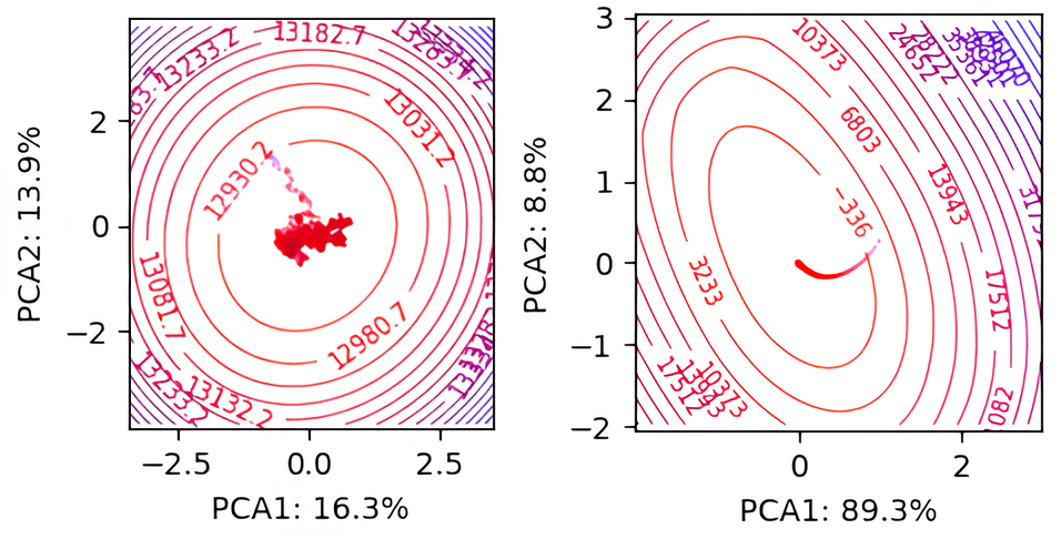
Figure 1: Projection of high-dimensional latent state trajectories under standard PC inference (right), and Langevin PC sampling (left), using normalised PCA trajectories. Latent state dynamics under Langevin PC result in a principled exploration of the posterior. More examples trajectories, and further details on how these were computed may be found in Appendix A.2. Contour lines and hue correspond to values of the negative log joint probability (blue high, red low), marker brightness corresponds to time-step (earlier is lighter).

$$d{\bm{Z}}_{t} =-\nabla_{{\bm{z}}}U({\bm{Z}}_{t})dt+\sqrt{2}d{\bm{W}}_{t}$$ (3)

where $${\bm{W}}_{t} \frac{e^{-U({\bm{z}})}}{\int_{\mathbb{R}^{d}}e^{-U({\bm{z}})}dz} U({\bm{z}}) -\log p({\mathbf{x}}^{(i)},{\mathbf{z}}|\boldsymbol{\theta}) {\mathbf{x}}^{(i)}$$ is a d-dimensional Brownian motion and admits a unique invariant density equal to under mild conditions. Setting the potential energy () to , for an observation gives us:

$$d{\bm{Z}}_{t} =\nabla_{{\bm{z}}}\log p({\mathbf{x}}^{(i)},{\bm{Z}}_{t}|\boldsymbol{\theta})dt+\sqrt{2}d{\bm{W}}_{t}$$ (4)

for which the corresponding Euler–Maruyama discretisation scheme is:

$${\bm{z}}^{(t)} ={\bm{z}}^{(t-1)}+\gamma\nabla_{{\bm{z}}}\log p({\bm{x}}^{(i)},{\bm{z}}^{(t-1)}|\boldsymbol{\theta})+\sqrt{2\gamma}\eta$$ (5)

with $\eta\sim\mathcal{N}(\boldsymbol{0},{\bm{I}})$. This is simply equal to a standard PC inference iteration (Equation 1) with the addition of some scaled Gaussian noise. With the inclusion of this Gaussian noise, the resultant iterates ${\bm{z}}^{(t)}$ would thus be interpretable as samples of the true model posterior, as $t\to\infty$, up to a bias induced by discretisation (Besage, J. E, 1994; Roberts & Tweedie, 1996).

Next, we note that by treating the (biased) samples from our Langevin chain as samples from an approximate posterior instead, we may compute gradients of a Monte Carlo estimate for the evidence lower-bound with respect to our model parameters $\boldsymbol{\theta}$:

$$\nabla_{\boldsymbol{\theta}}\mathcal{L}_{\text{ELBO}} =\nabla_{\boldsymbol{\theta}}\left[\mathbb{E}_{\tilde{p}({\mathbf{z}}|{\mathbf{x}})}[\log p({\mathbf{x}},{\mathbf{z}}|\boldsymbol{\theta})-\log\tilde{p}({\mathbf{z}}|{\mathbf{x}})]\right]$$ (6)

Where the approximate posterior $$\tilde{p}({\mathbf{z}}|{\mathbf{x}}) \boldsymbol{\theta}$$ corresponds to the empirical distribution of our Langevin chain. Because we are only interested in gradients with respect to our parameters , the intractable entropy term of our sample distribution may be ignored

$$=\nabla_{\boldsymbol{\theta}}\left[\mathbb{E}_{\tilde{p}({\mathbf{z}}|{\mathbf{x}})}[\log p({\mathbf{x}},{\mathbf{z}}|\boldsymbol{\theta})]\right]$$

$$\quad-\underbrace{\nabla_{\boldsymbol{\theta}}\left[\mathbb{E}_{\tilde{p}({\mathbf{z}}|{\mathbf{x}})}[\log\tilde{p}({\mathbf{z}}|{\mathbf{x}})]\right]}_{=0}$$ (7)

$$\approx\nabla_{\boldsymbol{\theta}}\frac{1}{T}\sum_{t}\log p({\bm{x}},{\bm{z}}^{(t)}|\boldsymbol{\theta})$$ (8)

Crucially, optimisation of this ELBO simply requires computing the gradient of our negative potential energy $\log p({\bm{x}},{\bm{z}}|\boldsymbol{\theta})$, with respect to $\boldsymbol{\theta}$ rather than ${\bm{z}}$, and is (computationally) identical to the learning step in Equation 2. From the perspective of neurobiological plausibility, this result is a pleasant surprise, as there already exists a substantial literature on how the dynamics described by Equation 1 and 2 may be implemented neuronally (Friston, 2003; 2005; Shipp, 2016; Bastos et al., 2012). Thus, the Langevin PC algorithm demands no additional neurobiological machinery other than the injection of Gaussian noise into our standard PC iterates. We briefly discuss the possible implications of this in Section 5.

From the perspective of an in-silico implementation, these gradients may be collected iteratively as the Markov chain is constructed, resulting in constant memory requirements independent of the chain length $T$, while reusing portions of the same backward pass used to compute our Langevin drift: $\nabla_{{\bm{z}}}\log p({\bm{x}},{\bm{z}}|\boldsymbol{\theta})$.

2.2 Amortised Warm-Starts

It is well-known that MCMC sampling methods, while powerful in theory, are notoriously sensitive to their choice of hyperparameters in practice (Steve Brooks, Andrew Gelman, Galin Jones, Xiao-Li Meng, 2011). One such choice is the state of initialisation for a Markov chain. A poor initialisation, far from the typical set of the invariant density will result in an inefficient chain with poor mixing time. This is of particular importance if we require constructing this Markov chain within each SGD training iteration. Traditional strategies to ameliorate this issue generally appeal to burn-in, i.e the discarding of a series of initial samples (Andrew Gelman et al., 2015), or by initialising at the MAP found via numerical optimisation (Salvatier et al., 2015). Such strategies are costly, particularly for our Langevin dynamics as they require expensive and wasted network evaluations.

We resolve this issue by training an amortised warm-up model (equivalently, an approximate inference model) conditional on observations. This allows us to provide a warm-start to our Langevin chain that is ideally within the typical set. In the context of the computational neuroscience origins of predictive coding, this formulations appeal compellingly to a dichotomy frequently identified in computational neuroscience. Namely, between fast but approximate feed-forward perception, vs slower but precise recurrent processing. The joint occurence of which, within the visual cortex in particular, has long been noted for it’s importance in object recognition (lamme_distinct_2000; mohsenzadeh_ultra-rapid_2018; kar_evidence_2019).

Architecturally this network may be chosen to resemble standard encoders, in encoder-decoder frameworks such as the VAE (Kingma & Welling, 2014), however the availability of (biased) samples from the model posterior obtained through Langevin dynamics afford us greater flexibility in how we train it. Here we propose and validate three objectives for training our amortised warm-start model: the forward KL, reverse KL and Jeffrey’s divergence.

2.2.1 Forward KL

Given Langevin samples from the model posterior, the most obvious objective for optimising our approximate inference network is the expected forward Kullback–Leibler divergence between the model posterior and our approximate posterior, with expectation approximated with mini-batches of observations. Specifically, the forward KL divergence can be separated into an intractable but encoder-independent entropy term, and a cross entropy term for which we may obtain a Monte Carlo estimate using our Langevin samples:

$$D_{\mathrm{KL}}(\tilde{p}({\mathbf{z}}|{\mathbf{x}})|q({\mathbf{z}}|{\mathbf{x}},\boldsymbol{\phi})) =\mathbb{E}_{(\tilde{p}({\mathbf{z}}|{\mathbf{x}})}\left[\log\frac{\tilde{p}({\mathbf{z}}|{\mathbf{x}})}{q({\mathbf{z}}|{\mathbf{x}},\boldsymbol{\phi})}\right]$$ (9)

where we are exclusively interested in obtaining gradients with respect to $\boldsymbol{\phi}$, and as such:

$$\!\!\!\!\!\!\nabla_{\boldsymbol{\phi}}D_{\mathrm{KL}}(\tilde{p}({\mathbf{z}}|{\mathbf{x}})|q({\mathbf{z}}|{\mathbf{x}},\boldsymbol{\phi})) =-\nabla_{\boldsymbol{\phi}}\mathbb{E}_{\tilde{p}({\mathbf{z}}|{\mathbf{x}})}\left[\log q({\mathbf{z}}|{\mathbf{x}},\boldsymbol{\phi})\right]$$

$$\quad\!\!+\underbrace{\nabla_{\boldsymbol{\phi}}\mathbb{E}_{\tilde{p}({\mathbf{z}}|{\mathbf{x}})}\left[\log\tilde{p}({\mathbf{z}}|{\mathbf{x}})\right]}_{0}$$ (10)

$$\!\!\!\!\!\!\!\!\!\!\!\!\!=-\nabla_{\boldsymbol{\phi}}\mathbb{E}_{\tilde{p}({\mathbf{z}}|{\mathbf{x}})}\left[\log q({\mathbf{z}}|{\mathbf{x}},\boldsymbol{\phi})\right]$$ (11)

which is simply the cross-entropy between our empirical Langevin posterior distribution and our approximate inference model. We will denote the Monte Carlo estimate for this approximate inference objective for a mini-batch of observations and a single batch of their associated posterior samples, as $\mathcal{L}_{A_{F}}({\bm{x}},{\bm{z}})$.

2.2.2 Reverse KL

While the forward KL is readily available given our access to samples from the posterior, its well-known moment matching behaviour may result in an initialisation at the average of multiple modes and as such a low posterior probability, particularly given the Gaussian approximate posterior we will be adopting (Bishop, 2006). In such circumstances, the mode matching behaviour of the reverse KL may be more appropriate. Computing the reverse KL divergence directly is difficult given our inability to directly evaluate the true log posterior probability. We can circumvent this by appealing to the standard ELBO, evaluated using the reparameterisation trick of Kingma & Welling (2014), which admits a decomposition consisting of an encoder-independent model evidence term, and the reverse KL we wish to obtain gradients from,

$$\mathcal{L}_{A_{R}} =D_{\mathrm{KL}}(q({\mathbf{z}}|{\mathbf{x}},\boldsymbol{\phi})|p({\mathbf{z}}|{\mathbf{x}}))$$ (12)

$$=\mathbb{E}_{q({\mathbf{z}}|{\mathbf{x}},\boldsymbol{\phi})}\left[\log\frac{q({\mathbf{z}}|{\mathbf{x}},\boldsymbol{\phi})}{p({\mathbf{z}}|{\mathbf{x}})}\right]$$ (13)

where we are once again exclusively interested in obtaining gradients with respect to $\boldsymbol{\phi}$, and as such,

$$\!\!\!\!\nabla_{\boldsymbol{\phi}}D_{\mathrm{KL}}( q({\mathbf{z}}|{\mathbf{x}},\boldsymbol{\phi})|p({\mathbf{z}}|{\mathbf{x}}))$$

$$=\nabla_{\boldsymbol{\phi}}\left[D_{\mathrm{KL}}(q({\mathbf{z}}|{\mathbf{x}},\boldsymbol{\phi})|p({\mathbf{z}}|{\mathbf{x}}))-\log p({\mathbf{x}})\right]$$ (14)

$$=\nabla_{\boldsymbol{\phi}}\left[-\mathbb{E}_{q({\mathbf{z}}|{\mathbf{x}},\boldsymbol{\phi})}[\log p({\mathbf{x}}|{\mathbf{z}})]\right.$$

$$\quad\qquad+\left.D_{\mathrm{KL}}(q({\mathbf{z}};\boldsymbol{\phi})|p({\mathbf{z}}))\right]$$ (15)

$$=\nabla_{\boldsymbol{\phi}}\mathcal{L}_{\text{ELBO}}$$ (16)

2.2.3 Jeffrey’s Divergence

By averaging gradients from the forward and reverse KL divergences we may also optimise with respect to (half) the Jeffrey’s divergence, also known as the symmetrised KL (Jeffreys, 1946), which can be shown to upper bound 4 times the Jensen-Shannon divergence (Lin, 1991).

$$\nabla_{\boldsymbol{\phi}}\mathcal{L}_{A_{J}} =\frac{1}{2}\nabla_{\boldsymbol{\phi}}\left[D_{\mathrm{KL}}(p({\mathbf{z}}|{\mathbf{x}})|q({\mathbf{z}}|{\mathbf{x}},\boldsymbol{\phi}))\right.$$

$$\quad+\left.D_{\mathrm{KL}}(q({\mathbf{z}}|{\mathbf{x}},\boldsymbol{\phi})|p({\mathbf{z}}|{\mathbf{x}}))\right]$$ (17)

2.3 Adaptive Preconditioning

There now exists a sizeable literature approaching gradient-based sampling from the perspective of optimisation in the space of probability measures (Jordan et al., 1998; Wibisono, 2018). This framing has led to the development of analogues to well-known methods from the classical optimisation literature, such as Nesterov’s acceleration (Ma et al., 2019). Similar analogues to preconditioning have also emerged in the literature, with (Girolami & Calderhead, 2011), demonstrating that an appropriately chosen, possibly position-specific, preconditioning matrix may be used to exploit the natural Riemannian geometry over the induced distributions, improving mixing time and sampling efficiency. A number of works have subsequently capitalized on this technique with a variety of Riemannian metrics, primarily within the context of stochastic gradient Langevin dynamics (SGLD) - a technique that applies Langevin dynamics to noisy mini-batch gradients over deep neural network parameters to obtain posterior samples (Welling & Teh, 2011; Ahn et al., 2012; Patterson & Teh, 2013; Li et al., 2015).

Here we adopt the adaptive second-moment computation of the Adam (Kingma & Ba, 2017) optimizer as our preconditioning matrix, computed with iterates over the log unnormalised probability $\log p({\mathbf{x}},{\mathbf{z}}_{t})$. The resultant algorithm may be considered analogous to the use of the diagonal RMSProp preconditioner for SGLD by Li et al. (2015), with key differences being in the use of a debiasing step, the use of non-stochastic gradients, and the inclusion of the gradient over the log prior in our second-moment calculations. We note that the Itô SDE associated with an overdamped Langevin diffusion with position-dependent metric tensor $G({\bm{X}}_{t})$, may be written as (Girolami & Calderhead, 2011; Ma et al., 2015; Roberts & Stramer, 2002; Xifara et al., 2014):

$$d{\bm{Z}}_{t}=G({\bm{X}}_{t})\nabla_{z}\log p({\mathbf{x}},{\mathbf{z}}|\boldsymbol{\theta})dt +\Gamma({\bm{Z}}_{t})dt$$ (18)

$$+\sqrt{2G({\bm{Z}}_{t})}d{\bm{W}}_{t}$$ (19)

where the term $\Gamma({\bm{Z}}_{t})$ accounts for changes in local curvature of the manifold, and is defined as:

$$\Gamma_{i}({\bm{Z}}_{t})=\sum_{j}\frac{G_{ij}({\bm{Z}}_{t})}{\partial Z_{j}}$$ (20)

The resultant discretization given by the Euler-Murayama scheme follows analogously to that in Equation 5. We follow identically to Ahn et al. (2012) and Li et al. (2015) and choose to ignore the $\Gamma_{i}({\bm{X}}_{t})$ term in our final discretized algorithm; valid under the assumption that our manifold changes slowly. Our final preconditioned algorithm with amortised warm-starts is described in Algorithm 1.

3 Related Works

Functionally similar algorithms to the one we propose here, have been independently developed from different theoretical perspectives (Hoffman, 2017; Taniguchi et al., 2022). Most notably, (Hoffman, 2017) proposed evolving latent states, also initialized by an inference network, using multiple iterations of Metropolis-adjusted Hamiltonian Monte Carlo (HMC) dynamics, with the final state being used to update the parameters of a generative model.

More recently, (Taniguchi et al., 2022) proposed the application of Metropolis-adjusted Langevin dynamics directly to the parameters of an amortisation network rather than datapoint-wise latent states, leveraging these iterates to also jointly learn a generative model or decoder network. Our work contributes to this growing literature by introducing an approach grounded in computational neuroscience, specifically through the lens of PC. Moreover, to the best of our knowledge, our work is the first to propose and empirically evaluate the use of the Forward KL and Jeffrey’s divergence as optimization objectives for a warm-start or inference network, as well as the adaptive preconditioning described herein for improving step size robustness in the unadjusted Langevin algorithm, particularly in the context of learning generative models.

4 Results

For all experiments considered here, we adopt generative and warm-start models that are largely coincident with the encoder, and decoder respectively from the VAE architecture of Higgins et al. (2016), with minor modifications, adopted from more recent VAE models (Child, 2021; Vahdat & Kautz, 2021), such as SiLU activation functions and softplus parameterised variances. Complete details of model architecture and hyperparameters can be found in Appendix A.1

Algorithm 1 Preconditioned Langevin PC with Amortized Warm-Starts trained with Jeffrey’s Divergence. For the version corresponding to warm-starts with just the reverse KL, remove the forward KL accumulation and the coefficient of $\frac{1}{2}$ from the reverse KL gradients.

0:  $\mathcal{D}$: Data-generating distribution

0:  $p({\mathbf{x}},{\mathbf{z}}|\boldsymbol{\theta})$: Generative model ($\boldsymbol{\theta}$)

0:  $q({\mathbf{z}}|{\mathbf{x}},\boldsymbol{\phi})$: Approximate inference model ($\boldsymbol{\phi}$)

0:  $\beta$: Preconditioning decay rate

0:  $\gamma,\alpha,T$: Langevin step size, parameter learning rate, and number of sampling steps

  for ${\mathbf{x}}\sim\mathcal{D}$ do

     ${\bm{g}}_{\boldsymbol{\theta}},{\bm{g}}_{\boldsymbol{\phi}},{\bm{m}}^{(0)}\leftarrow\boldsymbol{0}$

     ${\bm{z}}^{(0)}\sim q({\mathbf{z}}|{\bm{x}},\boldsymbol{\phi})$

     ${\bm{g}}_{\boldsymbol{\phi}}\mathrel{+}=\frac{1}{2}\nabla_{\boldsymbol{\phi}}\mathcal{L}_{A_{R}}$ $\triangleright$ Reverse KL gradients

     for $t\in\{1,2,\dots,T\}$ do

        ${\bm{g}}_{{\bm{z}}}\leftarrow\nabla_{{\bm{z}}}\log p({\mathbf{x}},{\bm{z}}^{(t-1)}|\boldsymbol{\theta})$ $\triangleright$ Drift

        ${\bm{m}}^{(t)}\leftarrow\beta\cdot{\bm{m}}^{(t-1)}+(1-\beta)\cdot({\bm{g}}_{{\bm{z}}}^{T}{\bm{g}}_{{\bm{z}}})$

        $\hat{{\bm{m}}}^{(t)}\leftarrow\sqrt{{\bm{m}}^{(t)}/(1-\beta^{t})}$ $\triangleright$ Bias correction

        ${\bm{z}}^{(t)}\leftarrow\gamma\cdot{\bm{g}}_{{\bm{z}}}\oslash\hat{{\bm{m}}}^{(t)}+\eta$, $\eta\sim\mathcal{N}(\boldsymbol{0},\text{diag}(2\gamma\cdot\hat{{\bm{m}}}))$

        ${\bm{g}}_{\boldsymbol{\theta}}\mathrel{+}=\nabla_{\boldsymbol{\theta}}\log p({\mathbf{x}},{\bm{z}}^{(t-1)}|\boldsymbol{\theta})$

        ${\bm{g}}_{\boldsymbol{\phi}}\mathrel{+}=\frac{1}{2T}\nabla_{\boldsymbol{\phi}}\mathcal{L}_{A_{F}}$ $\triangleright$ Forward KL gradients

     end for

     $\boldsymbol{\theta}\mathrel{+}=\alpha\cdot{\bm{g}}_{\boldsymbol{\theta}}$ $\triangleright$ Generative model update

     $\boldsymbol{\phi}\mathrel{+}=\alpha\cdot{\bm{g}}_{\boldsymbol{\phi}}$ $\triangleright$ Warm start model update

  end for

4.1 Approximate Inference Objectives

We begin by investigating the performance of our three approximate inference objectives, the forward KL, reverse KL and Jeffrey’s divergence on the quality of our samples when trained with CIFAR-10 (Krizhevsky, 2009), SVHN (Netzer et al., 2011) and CelebA (64x64) (Liu et al., 2015). As a baseline, we also test with no amortized warm-starts, instead using samples from our prior, for which we adopt an isotropic Gaussian with variance 1, to initialise our Langevin chain. For all tests, we also adopt this prior initialisation for the first 50 batches of training to ameliorate the effects of any poor initialisation in our warm-start models.

To quantify sample quality we compute the the standard Fréchet distance with Inceptionv3 representations (FID) (Heusel et al., 2017) using 50,000 samples. We observe a largely consistent relationship for the forward KL, with the objective exhibiting both poor performance in terms of sample quality and training instabilities resulting from an increasingly poor initialisation as training progresses. We validate this by recording changes in log probability and the L2 normed gradient of the log probability for random samples during their sampling trajectories for the three objectives. We observe significantly qualitatively different behaviours for the forward KL initialisations, observing drift-dominant conditions with dynamics dominated by maxima-seeking behaviour suggesting poor initialisation far from the mode. Example recordings of the change in log probability $\Delta\log p({\bm{x}},{\bm{z}})$ may be found in Figure 3. Further examples, and the equivalent normed gradient plots can be found in Appendix A.3.

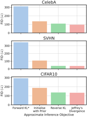
Figure 2: FID when using amortised warm-starts trained with our three approximate inference objectives, and baseline with no warm-start model, using initialisation with the prior. ^∗ Values for the forward KL objective are reported for 1 epoch due to the instability of this objective resulting in exploding gradients.

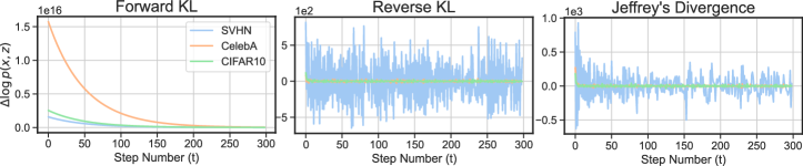
Figure 3: Changes in log probability ($\Delta\log p({\bm{x}},{\bm{z}})$) during Langevin sampling show forward KL initialisation results in long periods of drift-dominant conditions far from the mode.

In comparison we observe clear improvements in sample quality and FID when using amortised warm-starts trained with Jeffrey’s divergence or the reverse KL over the baseline encoder-only models. Due to the improved performance of the Jeffrey’s divergence objective in terms of the FID, and qualitatively more diverse sample quality, we adopt this objective for all subsequent experiments. FID values for the three objectives can be found in Figure 2, note that due to exploding gradients for the forward KL objective at later epochs, the FID values in for the forward KL correspond to performance at 1 epoch.

4.2 Preconditioning Induced Robustness

We assess the impact of preconditioning on increasing step sizes by testing models with and without preconditioning as we vary the Langevin step size from 0.001 to 0.5. We observe a substantial protective effect on the degradation of sample quality as step size increases in terms of the FID (Figure 4) of the resultant models, with the strength of this protective effect generally correlating with the strength of the preconditioning parameter $\beta$.

We also find that while preconditioned models exhibit better sample quality over their non-preconditioned counterparts, over the majority of step sizes tested, this trend begins to reverse at the very lowest Langevin step-sizes (1e-3), where non-preconditioned models reach parity or even improved performance. This relationship appears to mirror that of adaptive optimizers for SGD as used in practice, where adaptive optimizers exhibit greater robustness to a wide range of learning rates, but risk being outperformed by standard SGD optimization with a carefully finetuned learning rate.

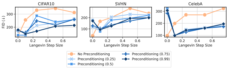
Figure 4: FID for Langevin PC models with and without preconditioning across different step-sizes. Numbers in brackets correspond to the preconditioning decay rate ($\beta$). Models trained with preconditioned Langevin dynamics experience significantly less degradation in sample quality at higher step-sizes. With stronger preconditioning generally correlating to the greatest robustness against inference learning rate.

4.3 Samples and Metrics

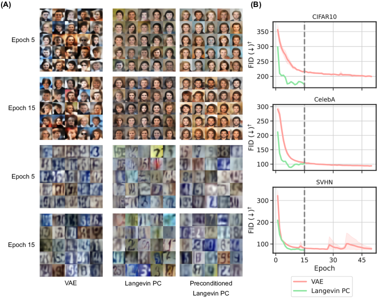
Figure 5: (A) Samples from identical generative models trained as VAEs (left), with LPC (middle), and with preconditioned LPC (right) on CelebA 64x64 (top), and SVHN (bottom). Epoch 50 samples for VAE models can be found in Appendix A.3. (B) Sample FID curves of VAE and LPC models throughout training. LPC models generally converge in significantly fewer epochs than their equivalent VAE trained models, with certain models converging in as few as 3 epochs. ^† Note: FID values reported in this graph are calculated online during training using significantly fewer samples than the post-training values reported in Table 1, and may thus differ in precise value.

We trained identical generative models using the standard VAE objective, alongside the LPC methodologies described herein. VAE models were hyperparameter tuned on learning rates with the best performing model with respect to FID being chosen for comparison. LPC models were analogously tuned on inference learning rate and preconditioning strength. Remaining hyperparameters were kept constant between runs such as optimizer, batch size and prior variance, to ensure a fair and like-for-like comparison. Full experimental details may be found in Appendix A.1, alongside the optimal hyperparameters selected for each dataset.

LPC and VAE models were trained for 15 and 50 epochs respectively. To evaluate sample quality we computed FID (using 50,000 samples), as well as density and coverage (Naeem et al., 2020) - a more robust alternative to precision and recall metrics - also using Inceptionv3 embeddings.

LPC models demonstrated comparative or better performance to their VAE counterparts. In particular, LPC models out-performed VAE models trained for more than 3 times as many SGD iterations (50 epochs vs 15), on SVHN and CIFAR10, in terms of FID, as well as on CelebA and CIFAR10 with respect to density and coverage. Samples from LPC models were also markedly less blurry - or more sharp - in comparison to VAE counterparts, an issue known to plague VAE models. (See Figure 5, for some non-cherry picked examples).

Table 1: Comparative evaluation of FID, Density, and Coverage for LPC and VAE models across different datasets.

Dataset	FID (↓)	Density (↑)	Coverage (↑)
LPC (15 Epochs)
CelebA	$97.49$	$0.54$	$0.13$
SVHN	$39.64$	$0.33$	$0.42$
CIFAR10	$113.29$	$0.63$	$0.13$
VAE (15 Epochs)
CelebA	$90.63$	$0.10$	$0.08$
SVHN	$53.88$	$0.60$	$0.39$
CIFAR10	$183.21$	$0.06$	$0.03$
VAE (50 Epochs)
CelebA	$82.09$	$0.16$	$0.12$
SVHN	$44.76$	$0.65$	$0.48$
CIFAR10	$145.87$	$0.14$	$0.06$

5 Discussion

We have presented an algorithm for training generic deep generative models that builds upon the PC framework of computational neuroscience and consists of three primary components: an unadjusted overdamped Langevin sampling, an amortised warm-start model, and an optional light-weight diagonal preconditioning. We have evaluated three different objectives for training our amortised warm-start model: the forward KL, reverse KL and the Jeffrey’s divergence, and found consistent improvements when using the reverse KL and Jeffrey’s divergence over baselines with no warm-starts (Figure 2). We have also evaluated our proposed form of adaptive preconditioning and observed an increased robustness to increaing Langevin step size (Figure 4). Finally, we have evaluated the resultant Langevin PC algorithm by training like-for-like models with the standard VAE methodology or the proposed Langevin PC algorithm. We have observed comparative or improved performance in a number of key metrics including sample quality, diversity and coverage (Table 1), while observing training convergence in a fraction of the number of SGD training iterations (Figure 5B).

5.1 Future directions

Langevin predictive coding opens doors in two different directions. The first is in regards to PC as an instantiation of the Bayesian brain hypothesis and as a candidate computational theory of cortical dynamics. In this setting, the introduction of Gaussian noise into the PC framework may represent more than simply an implementational detail associated with Langevin sampling but rather a deeper phenomena rooted in the ability of biological learning systems such as the brain to utilise sources of endogenous noise to their advantage.

It is well known that neuronal systems, including their dynamics and responses, are rife with noise at multiple levels (Faisal et al., 2008; Shadlen & Newsome, 1998). These sources of noise arise from, amongst other things, stochastic processes occuring at the sub-cellular level, impacting neuronal response through, for example, fluctuations in membrane-potential (Derksen & Verveen, 1966). Yet the precise role of such randomness, in information processing, continues to be an open question (McDonnell & Ward, 2011; Deco et al., 2013). The Langevin PC algorithm suggests one such role may be in the principled exploration of the latent space of hypotheses under one’s generative model.

Secondly, from the perspective of Langevin PC as an in-silico generative modelling algorithm we note a number of interesting avenues that we have not had the time to explore here. These include:

• Models with a hierarchy of stochastic variables, such as those found in most state of the art VAE models (Child, 2021; Vahdat & Kautz, 2021; Hazami et al., 2022). Which may require adopting a corresponding top-down hierarchical warm-start model.

• Automatic convergence criteria for determining when our Markov chain has converged to a certain level of error (Roy, 2020).

• Underdamped Langevin dynamics, which incorporate auxiliary momentum variables into the Langevin sampling to achieve an accelerated rate of convergence (Cheng et al., 2018; Ma et al., 2019).

5.2 Limitations

The methods we propose here are not without limitation. When implemented on current in-silico autograd frameworks, the need to enact multiple sequential iterations of Langevin dynamics for each SGD iteration requires additional computational cost and thus wall-clock time. In practice, this additional wall-clock time is counteracted, to an extent, by the increased efficiency of the Langevin PC algorithm in terms of the number of SGD iterations required to obtain similar or better performance as their VAE counterparts. When accounted for, we nonetheless observed end-to-end wall clock times for training that were approximately x7 and x11 slower for LPC algorithms using the reverse KL and Jeffrey’s divergence respectively. (See Appendix A.4 for per batch timings and relative slow downs).

We note that this additional cost is isolated to training, whereas the cost of sampling LPC models remain equivalent to their VAE counterparts - requiring a single ancestral sample, or forward evaluation, through the generative model to obtain. For models deployed for long-term use, such inference costs account for the bulk of computational cost. Therefore, LPC may be a viable candidate to improve model quality without increasing inference cost when deployed. We also speculate that the form of these dynamics - precision-weighted prediction errors with additive Gaussian noise - may render them a good candidate for implementation on analog hardware, where such dynamics would be enacted by the intrinsic but noisy fast-timescale physics of such systems.

Appendix A Appendix

A.1 Experimental Details

All experiments in this paper adopted the following network architectures for the generative model and approximate inference models. These models are derived from the encoder/decoder VAE architectures of (Higgins et al., 2016) with slight modifications such as the use of the SiLU activation function adopted in more recent VAE models such as (Hazami et al., 2022; Vahdat & Kautz, 2021).

Generative Model ($\log p({\mathbf{x}},{\mathbf{z}}|\boldsymbol{\theta})$	Warm-Start/Encoder Model ($\log q({\mathbf{z}}|{\mathbf{x}},\phi)$)
Latent Dim = 40	Obs Dim = (64, 64) or (32, 32) or (28, 28)
Linear(256)	If Input = (64,64): Conv(32, 3, 3, 1)
else: Conv(32)
SiLU	SiLU
Conv(64, 4, 1, 0)	Conv(32)
SiLU	SiLU
Conv(64)	Conv(64)
SiLU	SiLU
Conv(32)	If Obs Dim = (28, 28): Conv(64, 3)
else: Conv(64)
SiLU	SiLU
If obs dim = (64, 64): Conv(32)
else if obs dim = (28, 28): Conv(32, 3, 1, 0)
else: Conv(32, 3, 1, 1)	Conv(256, 4)
SiLU	SiLU
Conv(3)	Linear(2*40)
(Softplus(beta=0.3) applied to variance component)

Table 2: Layer argument definitions are Conv(Number of out channels, kernel size, stride, padding), and Linear(Output dimensions) for 2d convolution and linear layers respectively. Kernel size, stride and padding are 4x4, 2, and 1 respectively if not explicitly stated.

Hyperparameter	Value
Optimizer	Adam
Learning Rate ($\alpha$)	1e-3
Batch size	64
Output Likelihood	Discretised Gaussian
Max Sampling Steps ($T$)	300
Preconditioning Decay Rate ($\beta$)	0.99

Table 3: Default hyperparameters used in experiments unless explicitly stated. Note: some of these are varied as part of ablation tests, see main text for more details.

Optimal learning rates for VAE were found to be 1e-3, 8e-4 and 1e-3 for CIFAR10, CelebA and SVHN respectively. For LPC, optimal inference learning rates were found to be 1e-1, 1e-1, and 1e-3 with $\beta$ equal to 0.25, 0.25 and 0 (No preconditioning), for CIFAR10, CelebA and SVHN respectively.

A.2 Low-Dimensional Projection of Inference and Sampling Trajectories

The problem of visualising high-dimensional trajectories is a well-known one which generally arises in the context of visualising the stochastic gradient descent trajectories of high-dimensional weights in neural networks (Gallagher & Downs, 2003; Li et al., 2017; Lipton, 2016).

Here we adapt the method suggested by (Li et al., 2017) to visualise the inference or sampling trajectories of our latent states ${\mathbf{z}}^{(t)}$. We apply principle component analysis (PCA) to the series of vectors pointing from our final state to our intermediate states, i.e. $[{\mathbf{z}}^{(1)}-{\mathbf{z}}^{(T)},\dots,{\mathbf{z}}^{(T-1)}-{\mathbf{z}}^{(T)}]$, and project our trajectories on the first two principle components. We visualise the projected trajectories on top of the loss landscape of the negative potential (log joint probability) by evaluating our generative model across a grid of latent states linearly interpolated in the direction of the principle components around the final state.

Projections of an example batch of sampling trajectories can be seen in Figure 6.

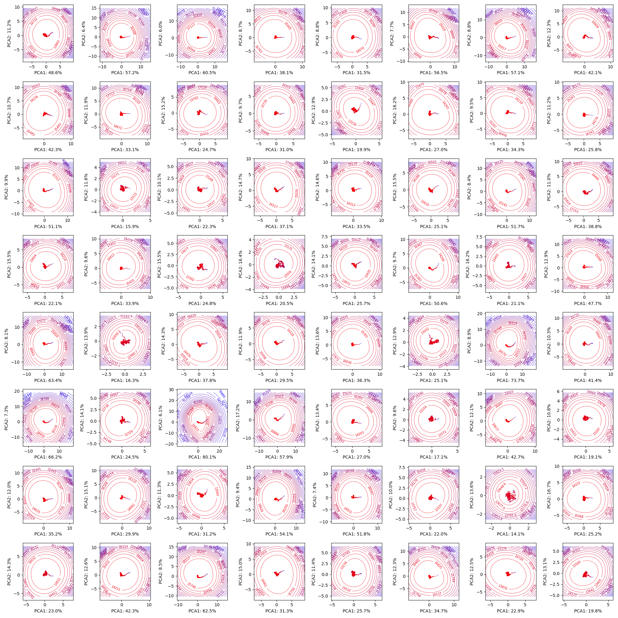
Figure 6: Projection of a 64 sample batched high-dimensional latent state trajectories under Langevin PC sampling. Contour lines and hue correspond to values of the negative log joint probability (blue high, red low), marker brightness corresponds to time-step (earlier is lighter).

A.3 Additional Samples and Figures

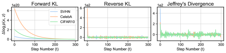
Figure 7: Log probability changes during Langevin sampling for samples from training batch 600 for our three approximate inference objectives.

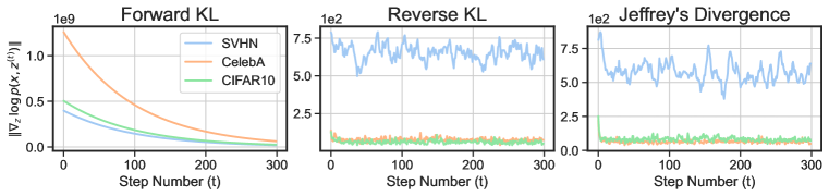
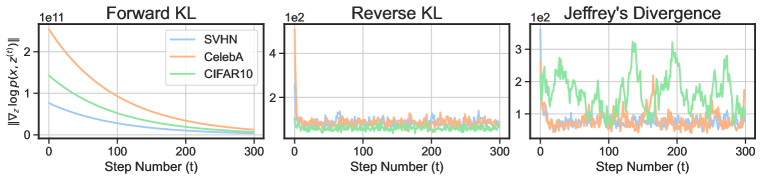
Figure 8: L2 normed log probability during Langevin sampling for samples from training batch 300 (top) and 600 (bottom), for our three approximate inference objectives.

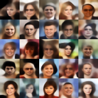
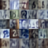
Figure 9: Epoch 50 samples from VAEs trained on CelebA 64x64 (left), and SVHN (right)

A.4 Wall Clock Time

Table 4: Batch times and end to end slowdowns for LPC algorithms as recorded on an Nvidia 4090. End to end refers to 15 epochs for LPC algorithms, and 50 epochs for VAE algorithms.

Algorithm	Per batch time (ms)	Per batch slowdown	End to end slowdown
VAE	0.022	x1	x1
LPC (Reverse)	0.533	x24	x7
LPC (Jeffreys)	0.798	x36	x11

References

- Ahn et al. (2012) Sungjin Ahn, Anoop Korattikara, and Max Welling. Bayesian Posterior Sampling via Stochastic Gradient Fisher Scoring, June 2012. URL http://arxiv.org/abs/1206.6380. arXiv:1206.6380 [cs, stat].
- Andrew Gelman et al. (2015) Andrew Gelman, John B. Carlin, Hal S. Stern, David B. Dunson, Aki Vehtari, and Donald B. Rubin. Bayesian Data Analysis. Chapman and Hall/CRC, New York, 3 edition, July 2015. ISBN 978-0-429-11307-9. doi: 10.1201/b16018.
- Bastos et al. (2012) Andre M. Bastos, W. Martin Usrey, Rick A. Adams, George R. Mangun, Pascal Fries, and Karl J. Friston. Canonical microcircuits for predictive coding. Neuron, 76(4):695–711, November 2012. ISSN 1097-4199. doi: 10.1016/j.neuron.2012.10.038.
- Besage, J. E (1994) Besage, J. E. Discussion of the paper by grenander and miller. Journal of the Royal Statistical Society: Series B (Methodological), 56(4):581–603, 1994. doi: https://doi.org/10.1111/j.2517-6161.1994.tb02001.x. URL https://rss.onlinelibrary.wiley.com/doi/abs/10.1111/j.2517-6161.1994.tb02001.x. tex.eprint: https://rss.onlinelibrary.wiley.com/doi/pdf/10.1111/j.2517-6161.1994.tb02001.x.
- Bishop (2006) Christopher M. Bishop. Pattern recognition and machine learning. Springer-Verlag, Berlin, Heidelberg, 2006. ISBN 0-387-31073-8.
- Bogacz (2017) Rafal Bogacz. A tutorial on the free-energy framework for modelling perception and learning. Journal of Mathematical Psychology, 76:198–211, February 2017. ISSN 0022-2496. doi: 10.1016/j.jmp.2015.11.003. URL https://www.sciencedirect.com/science/article/pii/S0022249615000759.
- Cheng et al. (2018) Xiang Cheng, Niladri S. Chatterji, Peter L. Bartlett, and Michael I. Jordan. Underdamped Langevin MCMC: A non-asymptotic analysis, January 2018. URL http://arxiv.org/abs/1707.03663. arXiv:1707.03663 [cs, stat].
- Child (2021) Rewon Child. Very Deep VAEs Generalize Autoregressive Models and Can Outperform Them on Images, March 2021. URL http://arxiv.org/abs/2011.10650. arXiv:2011.10650 [cs].
- Clark (2013) Andy Clark. Whatever next? Predictive brains, situated agents, and the future of cognitive science. Behavioral and Brain Sciences, 36(3):181–204, June 2013. ISSN 0140-525X, 1469-1825. doi: 10.1017/S0140525X12000477. Publisher: Cambridge University Press.
- Deco et al. (2013) Gustavo Deco, Viktor K. Jirsa, and Anthony R. McIntosh. Resting brains never rest: computational insights into potential cognitive architectures. Trends in Neurosciences, 36(5):268–274, May 2013. ISSN 1878-108X. doi: 10.1016/j.tins.2013.03.001.
- Derksen & Verveen (1966) H. E. Derksen and A. A. Verveen. Fluctuations of Resting Neural Membrane Potential. Science, 151(3716):1388–1389, March 1966. doi: 10.1126/science.151.3716.1388. URL https://www.science.org/doi/10.1126/science.151.3716.1388. Publisher: American Association for the Advancement of Science.
- Faisal et al. (2008) A. Aldo Faisal, Luc P. J. Selen, and Daniel M. Wolpert. Noise in the nervous system. Nature Reviews Neuroscience, 9(4):292–303, April 2008. ISSN 1471-0048. doi: 10.1038/nrn2258. URL https://www.nature.com/articles/nrn2258. Number: 4 Publisher: Nature Publishing Group.
- Feldman & Friston (2010) Harriet Feldman and Karl Friston. Attention, Uncertainty, and Free-Energy. Frontiers in Human Neuroscience, 4:215, 2010. ISSN 1662-5161. doi: 10.3389/fnhum.2010.00215. URL https://www.frontiersin.org/article/10.3389/fnhum.2010.00215.
- Fountas et al. (2022) Zafeirios Fountas, Anastasia Sylaidi, Kyriacos Nikiforou, Anil K. Seth, Murray Shanahan, and Warrick Roseboom. A Predictive Processing Model of Episodic Memory and Time Perception. Neural Computation, 34(7):1501–1544, June 2022. ISSN 0899-7667. doi: 10.1162/neco˙a˙01514. URL https://doi.org/10.1162/neco_a_01514.
- Friston (2003) Karl Friston. Learning and inference in the brain. Neural Networks, 16(9):1325–1352, November 2003. ISSN 08936080. doi: 10.1016/j.neunet.2003.06.005. URL https://linkinghub.elsevier.com/retrieve/pii/S0893608003002454.
- Friston (2005) Karl Friston. A theory of cortical responses. Philosophical Transactions of the Royal Society B: Biological Sciences, 360(1456):815–836, April 2005. ISSN 0962-8436. doi: 10.1098/rstb.2005.1622. URL https://www.ncbi.nlm.nih.gov/pmc/articles/PMC1569488/.
- Friston (2018) Karl Friston. Does predictive coding have a future? Nature Neuroscience, 21(8):1019–1021, August 2018. ISSN 1546-1726. doi: 10.1038/s41593-018-0200-7. URL https://www.nature.com/articles/s41593-018-0200-7. Bandiera_abtest: a Cg_type: Nature Research Journals Number: 8 Primary_atype: News & Views Publisher: Nature Publishing Group Subject_term: Computational neuroscience;Neural circuits;Neuronal physiology Subject_term_id: computational-neuroscience;neural-circuit;neuronal-physiology.
- Friston & Kiebel (2009) Karl Friston and Stefan Kiebel. Predictive coding under the free-energy principle. Philosophical Transactions of the Royal Society of London. Series B, Biological Sciences, 364(1521):1211–1221, May 2009. ISSN 1471-2970. doi: 10.1098/rstb.2008.0300.
- Gallagher & Downs (2003) M. Gallagher and T. Downs. Visualization of learning in multilayer perceptron networks using principal component analysis. IEEE transactions on systems, man, and cybernetics. Part B, Cybernetics: a publication of the IEEE Systems, Man, and Cybernetics Society, 33(1):28–34, 2003. ISSN 1083-4419. doi: 10.1109/TSMCB.2003.808183.
- Girolami & Calderhead (2011) Mark Girolami and Ben Calderhead. Riemann manifold Langevin and Hamiltonian Monte Carlo methods. Journal of the Royal Statistical Society: Series B (Statistical Methodology), 73(2):123–214, 2011. ISSN 1467-9868. doi: 10.1111/j.1467-9868.2010.00765.x. URL https://onlinelibrary.wiley.com/doi/abs/10.1111/j.1467-9868.2010.00765.x. _eprint: https://onlinelibrary.wiley.com/doi/pdf/10.1111/j.1467-9868.2010.00765.x.
- Hazami et al. (2022) Louay Hazami, Rayhane Mama, and Ragavan Thurairatnam. Efficient-VDVAE: Less is more, April 2022. URL http://arxiv.org/abs/2203.13751. arXiv:2203.13751 [cs].
- Heusel et al. (2017) Martin Heusel, Hubert Ramsauer, Thomas Unterthiner, Bernhard Nessler, and Sepp Hochreiter. GANs Trained by a Two Time-Scale Update Rule Converge to a Local Nash Equilibrium, June 2017. URL https://arxiv.org/abs/1706.08500v6.
- Higgins et al. (2016) Irina Higgins, Loic Matthey, Arka Pal, Christopher Burgess, Xavier Glorot, Matthew Botvinick, Shakir Mohamed, and Alexander Lerchner. beta-VAE: Learning Basic Visual Concepts with a Constrained Variational Framework. November 2016. URL https://openreview.net/forum?id=Sy2fzU9gl.
- Hoffman (2017) Matthew D. Hoffman. Learning Deep Latent Gaussian Models with Markov Chain Monte Carlo. In Proceedings of the 34th International Conference on Machine Learning, pp. 1510–1519. PMLR, July 2017. URL https://proceedings.mlr.press/v70/hoffman17a.html. ISSN: 2640-3498.
- Hoffman & Gelman (2011) Matthew D. Hoffman and Andrew Gelman. The No-U-Turn Sampler: Adaptively Setting Path Lengths in Hamiltonian Monte Carlo, November 2011. URL http://arxiv.org/abs/1111.4246. arXiv:1111.4246 [cs, stat].
- Hohwy et al. (2008) Jakob Hohwy, Andreas Roepstorff, and Karl Friston. Predictive coding explains binocular rivalry: an epistemological review. Cognition, 108(3):687–701, September 2008. ISSN 0010-0277. doi: 10.1016/j.cognition.2008.05.010.
- Hosoya et al. (2005) Toshihiko Hosoya, Stephen A. Baccus, and Markus Meister. Dynamic predictive coding by the retina. Nature, 436(7047):71–77, July 2005. ISSN 1476-4687. doi: 10.1038/nature03689.
- Jeffreys (1946) Harold Jeffreys. An Invariant Form for the Prior Probability in Estimation Problems. Proceedings of the Royal Society of London. Series A, Mathematical and Physical Sciences, 186(1007):453–461, 1946. ISSN 0080-4630. URL https://www.jstor.org/stable/97883. Publisher: The Royal Society.
- Jordan et al. (1998) Richard Jordan, David Kinderlehrer, and Felix Otto. The Variational Formulation of the Fokker–Planck Equation. SIAM Journal on Mathematical Analysis, 29(1):1–17, January 1998. ISSN 0036-1410. doi: 10.1137/S0036141096303359. URL https://epubs.siam.org/doi/abs/10.1137/S0036141096303359. Publisher: Society for Industrial and Applied Mathematics.
- Kanai et al. (2015) Ryota Kanai, Yutaka Komura, Stewart Shipp, and Karl Friston. Cerebral hierarchies: predictive processing, precision and the pulvinar. Philosophical Transactions of the Royal Society B: Biological Sciences, 370(1668):20140169, May 2015. doi: 10.1098/rstb.2014.0169. URL https://royalsocietypublishing.org/doi/10.1098/rstb.2014.0169. Publisher: Royal Society.
- Kingma & Ba (2017) Diederik P. Kingma and Jimmy Ba. Adam: A Method for Stochastic Optimization, January 2017. URL http://arxiv.org/abs/1412.6980. arXiv:1412.6980 [cs].
- Kingma & Welling (2014) Diederik P. Kingma and Max Welling. Auto-Encoding Variational Bayes. arXiv:1312.6114 [cs, stat], May 2014. URL http://arxiv.org/abs/1312.6114. arXiv: 1312.6114.
- Krizhevsky (2009) Alex Krizhevsky. Learning Multiple Layers of Features from Tiny Images. 2009. URL https://api.semanticscholar.org/CorpusID:18268744.
- Li et al. (2015) Chunyuan Li, Changyou Chen, David Carlson, and Lawrence Carin. Preconditioned Stochastic Gradient Langevin Dynamics for Deep Neural Networks, December 2015. URL http://arxiv.org/abs/1512.07666. arXiv:1512.07666 [stat].
- Li et al. (2017) Hao Li, Zheng Xu, Gavin Taylor, Christoph Studer, and Tom Goldstein. Visualizing the Loss Landscape of Neural Nets, December 2017. URL https://arxiv.org/abs/1712.09913v3.
- Lin (1991) J. Lin. Divergence measures based on the Shannon entropy. IEEE Transactions on Information Theory, 37(1):145–151, January 1991. ISSN 1557-9654. doi: 10.1109/18.61115. Conference Name: IEEE Transactions on Information Theory.
- Lipton (2016) Zachary C. Lipton. Stuck in a What? Adventures in Weight Space, February 2016. URL http://arxiv.org/abs/1602.07320. arXiv:1602.07320 [cs].
- Liu et al. (2015) Ziwei Liu, Ping Luo, Xiaogang Wang, and Xiaoou Tang. Deep Learning Face Attributes in the Wild. In Proceedings of International Conference on Computer Vision (ICCV), December 2015.
- Ma et al. (2015) Yi-An Ma, Tianqi Chen, and Emily B. Fox. A Complete Recipe for Stochastic Gradient MCMC, October 2015. URL http://arxiv.org/abs/1506.04696. arXiv:1506.04696 [math, stat].
- Ma et al. (2019) Yi-An Ma, Niladri Chatterji, Xiang Cheng, Nicolas Flammarion, Peter Bartlett, and Michael I. Jordan. Is There an Analog of Nesterov Acceleration for MCMC?, October 2019. URL http://arxiv.org/abs/1902.00996. arXiv:1902.00996 [cs, math, stat].
- McDonnell & Ward (2011) Mark D. McDonnell and Lawrence M. Ward. The benefits of noise in neural systems: bridging theory and experiment. Nature Reviews Neuroscience, 12(7):415–425, July 2011. ISSN 1471-0048. doi: 10.1038/nrn3061. URL https://www.nature.com/articles/nrn3061. Number: 7 Publisher: Nature Publishing Group.
- Millidge et al. (2020) Beren Millidge, Alexander Tschantz, and Christopher L. Buckley. Predictive Coding Approximates Backprop along Arbitrary Computation Graphs. arXiv:2006.04182 [cs], October 2020. URL http://arxiv.org/abs/2006.04182. arXiv: 2006.04182.
- Mumford (1992) D. Mumford. On the computational architecture of the neocortex. II. The role of cortico-cortical loops. Biological Cybernetics, 66(3):241–251, 1992. ISSN 0340-1200. doi: 10.1007/BF00198477.
- Naeem et al. (2020) Muhammad Ferjad Naeem, Seong Joon Oh, Youngjung Uh, Yunjey Choi, and Jaejun Yoo. Reliable Fidelity and Diversity Metrics for Generative Models, February 2020. URL https://arxiv.org/abs/2002.09797v2.
- Neal (2011) Radford M. Neal. MCMC using Hamiltonian dynamics. May 2011. doi: 10.1201/b10905. URL http://arxiv.org/abs/1206.1901. arXiv:1206.1901 [physics, stat].
- Netzer et al. (2011) Yuval Netzer, Tao Wang, Adam Coates, Alessandro Bissacco, Bo Wu, and Andrew Y. Ng. Reading Digits in Natural Images with Unsupervised Feature Learning. In NIPS Workshop on Deep Learning and Unsupervised Feature Learning 2011, 2011. URL http://ufldl.stanford.edu/housenumbers/nips2011_housenumbers.pdf.
- Patterson & Teh (2013) Sam Patterson and Yee Whye Teh. Stochastic Gradient Riemannian Langevin Dynamics on the Probability Simplex. In Advances in Neural Information Processing Systems, volume 26. Curran Associates, Inc., 2013. URL https://proceedings.neurips.cc/paper/2013/hash/309928d4b100a5d75adff48a9bfc1ddb-Abstract.html.
- Pouget et al. (2013) Alexandre Pouget, Jeffrey M. Beck, Wei Ji Ma, and Peter E. Latham. Probabilistic brains: knowns and unknowns. Nature Neuroscience, 16(9):1170–1178, September 2013. ISSN 1546-1726. doi: 10.1038/nn.3495. URL https://www.nature.com/articles/nn.3495. Number: 9 Publisher: Nature Publishing Group.
- Rao & Ballard (1999) Rajesh P. N. Rao and Dana H. Ballard. Predictive coding in the visual cortex: a functional interpretation of some extra-classical receptive-field effects. Nature Neuroscience, 2(1):79–87, January 1999. ISSN 1546-1726. doi: 10.1038/4580. URL https://www.nature.com/articles/nn0199_79. Number: 1 Publisher: Nature Publishing Group.
- Roberts & Stramer (2002) G. O. Roberts and O. Stramer. Langevin Diffusions and Metropolis-Hastings Algorithms. Methodology And Computing In Applied Probability, 4(4):337–357, December 2002. ISSN 1573-7713. doi: 10.1023/A:1023562417138. URL https://doi.org/10.1023/A:1023562417138.
- Roberts & Rosenthal (1998) Gareth O. Roberts and Jeffrey S. Rosenthal. Optimal scaling of discrete approximations to Langevin diffusions. Journal of the Royal Statistical Society: Series B (Statistical Methodology), 60(1):255–268, 1998. ISSN 1467-9868. doi: 10.1111/1467-9868.00123. URL https://onlinelibrary.wiley.com/doi/abs/10.1111/1467-9868.00123. _eprint: https://onlinelibrary.wiley.com/doi/pdf/10.1111/1467-9868.00123.
- Roberts & Tweedie (1996) Gareth O. Roberts and Richard L. Tweedie. Exponential convergence of Langevin distributions and their discrete approximations. Bernoulli, 2(4):341–363, December 1996. ISSN 1350-7265. URL https://projecteuclid.org/journals/bernoulli/volume-2/issue-4/Exponential-convergence-of-Langevin-distributions-and-their-discrete-approximations/bj/1178291835.full. Publisher: Bernoulli Society for Mathematical Statistics and Probability.
- Rossky et al. (1978) P. J. Rossky, J. D. Doll, and H. L. Friedman. Brownian dynamics as smart Monte Carlo simulation. The Journal of Chemical Physics, 69(10):4628–4633, November 1978. ISSN 0021-9606. doi: 10.1063/1.436415. URL https://aip.scitation.org/doi/10.1063/1.436415. Publisher: American Institute of Physics.
- Roy (2020) Vivekananda Roy. Convergence Diagnostics for Markov Chain Monte Carlo. Annual Review of Statistics and Its Application, 7(1):387–412, 2020. doi: 10.1146/annurev-statistics-031219-041300. URL https://doi.org/10.1146/annurev-statistics-031219-041300. _eprint: https://doi.org/10.1146/annurev-statistics-031219-041300.
- Salvatier et al. (2015) John Salvatier, Thomas Wiecki, and Christopher Fonnesbeck. Probabilistic Programming in Python using PyMC, July 2015. URL https://arxiv.org/abs/1507.08050v1.
- Shadlen & Newsome (1998) Michael N. Shadlen and William T. Newsome. The Variable Discharge of Cortical Neurons: Implications for Connectivity, Computation, and Information Coding. Journal of Neuroscience, 18(10):3870–3896, May 1998. ISSN 0270-6474, 1529-2401. doi: 10.1523/JNEUROSCI.18-10-03870.1998. URL https://www.jneurosci.org/content/18/10/3870. Publisher: Society for Neuroscience Section: ARTICLE.
- Shipp (2016) Stewart Shipp. Neural Elements for Predictive Coding. Frontiers in Psychology, 7:1792, 2016. ISSN 1664-1078. doi: 10.3389/fpsyg.2016.01792. URL https://www.frontiersin.org/article/10.3389/fpsyg.2016.01792.
- Steve Brooks, Andrew Gelman, Galin Jones, Xiao-Li Meng (2011) Steve Brooks, Andrew Gelman, Galin Jones, Xiao-Li Meng (ed.). Handbook of Markov Chain Monte Carlo. Chapman and Hall/CRC, New York, May 2011. ISBN 978-0-429-13850-8. doi: 10.1201/b10905.
- Taniguchi et al. (2022) Shohei Taniguchi, Yusuke Iwasawa, Wataru Kumagai, and Yutaka Matsuo. Langevin Autoencoders for Learning Deep Latent Variable Models, September 2022. URL https://arxiv.org/abs/2209.07036v2.
- Vahdat & Kautz (2021) Arash Vahdat and Jan Kautz. NVAE: A Deep Hierarchical Variational Autoencoder, January 2021. URL http://arxiv.org/abs/2007.03898. arXiv:2007.03898 [cs, stat].
- Welling & Teh (2011) M. Welling and Y. Teh. Bayesian Learning via Stochastic Gradient Langevin Dynamics. June 2011. URL https://www.semanticscholar.org/paper/Bayesian-Learning-via-Stochastic-Gradient-Langevin-Welling-Teh/aeed631d6a84100b5e9a021ec1914095c66de415.
- Wibisono (2018) Andre Wibisono. Sampling as optimization in the space of measures: The Langevin dynamics as a composite optimization problem, June 2018. URL http://arxiv.org/abs/1802.08089. arXiv:1802.08089 [cs, math, stat].
- Xifara et al. (2014) Tatiana Xifara, Chris Sherlock, Samuel Livingstone, Simon Byrne, and Mark Girolami. Langevin diffusions and the Metropolis-adjusted Langevin algorithm. Statistics & Probability Letters, 91:14–19, August 2014. ISSN 01677152. doi: 10.1016/j.spl.2014.04.002. URL http://arxiv.org/abs/1309.2983. arXiv:1309.2983 [math, stat].
- Zahid et al. (2023a) Umais Zahid, Qinghai Guo, and Zafeirios Fountas. Predictive Coding as a Neuromorphic Alternative to Backpropagation: A Critical Evaluation, April 2023a. URL http://arxiv.org/abs/2304.02658. arXiv:2304.02658 [cs, q-bio].
- Zahid et al. (2023b) Umais Zahid, Guo Qinghai, and Zafeirios Fountas. Curvature-Sensitive Predictive Coding with Approximate Laplace Monte Carlo, March 2023b.