Twisted Magnetic Knots and Links

Abstract

For magnetic knots and links in plasmas we introduce an internal twist and study their dynamical behavior in numerical simulations. We use a set of helical and non-helical configurations and add an internal twist that cancels the helicity of the helical configurations or makes a non-helical system helical. These fields are then left to relax in a magnetohydrodynamic environment. In line with previous works we confirm the importance of magnetic helicity in field relaxation. However, an internal twist, as could be observed in coronal magnetic loops, does not just add or subtract helicity, but also introduces an alignment of the magnetic field with the electric current, which is the source term for helicity. This source term is strong enough to lead to a significant change of magnetic helicity, which for some cases leads to a loss of the stabilizing properties expressed in the realizability condition. Even a relatively weak internal twist in these magnetic fields leads to a strong enough source term for magnetic helicity that for various cases even in a low diffusion environment we observe an inversion in sign of magnetic helicity within time scales much shorter than the diffusion time. We conclude that in solar and stellar fields an internal twist does not automatically result in a structurally stable configuration and that the alignment of the magnetic field with the electric current must be taken into account.

I Introduction

The majority (over $99$%) of the observable matter in the universe is known to be in a state of plasma. Being a plasma, the electric conductivity is generally high and we observe electric currents and the magnetic fields these currents generate. These magnetic fields have been observed in planets, our Sun, stars, magnetars and galaxies.

Through the Lorentz force the magnetic field acts on the medium. At the same time, the motions of the medium leads to a change in electric current and the magnetic field. This non-linear interaction gives rise to various physically relevant effects. For instance, it can be used to explain the exponential amplification of a weak magnetic field (dynamo effect) in stars and galaxies (see e.g. Krause-Radler-1971-SolMagFields, ; BrandenbSubramanianReview2005, ). Other phenomena for which this interaction is crucial are solar coronal mass ejections (e.g. Barnes-2007-670-L53-ApJL, ) and stellar flares (e.g. Schrijver2009AdSpR43, ).

For laboratory and astrophysical plasmas we know that magnetic fields and electric currents have a significant effect on the dynamics and evolution of the system (e.g. MoffattBook1978, ; Biskamp-2003-Magnetohydrodynamic_Turbulence, ; Priest-2014-MHDSun, ). This is particularly true for magnetically dominated regions like the solar corona (Kasper-Klein-2021-127-8-PRL, ) where the magnetic pressure is larger than the hydrostatic pressure and magnetic forces dominate. In laboratory devices, the magnetic field is particularly important in confining hot plasmas in fusion devices like tokamaks or the Large Helical Device in Toki (Motojima2006LHD, ).

During solar maxima we can observe large-scale magnetic flux tubes on the solar surface (e.g. Ballegooijen-2004-612-519-ApJ, ). Those are a result of the dynamo action within the Sun which is responsible for the 11 year solar cycle. While the plasma motions give rise to particular magnetic field structure, the magnetic field in turn affects the plasma motions. Here, the geometry of the field lines plays an important role in the dynamics. For instance, a strong magnetic flux tube will rise due to magnetic buoyancy and a high curvature in the field lines gives rise to additional Lorentz forces. Finally, reconnection events near magnetic null points (Filippov-1999-185-2-SolPhys, ) (where the magnetic field vanishes) give rise to strong particle acceleration Pontin-Hornig-2005-99-77-GApFD .

While it should be evident that the field’s geometry affects the dynamics, it is less evident that its topology, i.e. field line connectivity, has a strong effect. The most used quantifier for the magnetic field topology is the magnetic helicity, which measures the linkage, twisting, braiding and knottedness of the magnetic field (MoffattBook1978, ). For astrophysical parameter regimes we know that this quantity changes on much longer time scales than the dynamics of the system. For instance, we have 11 years for the solar magnetic cycle, which compares to millions of years for the magnetic helicity decay time (e.g. BrandenbSubramanianReview2005, ).

This conservation has dramatic consequences for the plasma dynamics. For a freely relaxing field Woltjer-1958-489-91-PNAS, derived a minimum energy state with the restriction of magnetic helicity conservation. This state has the form of a linear force-free field with vanishing Lorentz force. Calculations by Taylor-1974-PrlE, and Taylor1986, in the fusion plasma context showed that a minimum energy state is a non-linear force-free state. ArnoldHopf1986, then demonstrated that the magnetic energy is bound from below by the presence of magnetic helicity, the so called realizability condition. This puts severe restrictions on the final equilibrium state, and the intermediate states the system is allowed to go through during its evolution.

Magnetic helicity is also being exploited in turbulent dynamo theory. In a turbulent plasma it has been shown (e.g. Frisch-Pouquet-Leorat-1975-JFluidMech, ; KleeorinRuzmaikin82, ; alpha2_periodic13, ) that helicity conservation leads to an inverse cascade where small-scale magnetic energy is transformed into large-scale energy. As a result, an initially weak small-scale magnetic field is being transformed into a strong large-scale field. This effect has been used to explain the existence of strong large-scale magnetic fields in planets, stars and galaxies.

Following these early analytical results and with the rise of computing power, various numerical calculations on magnetic field relaxation have been performed. Ideal magnetohydrodynamics (MHD) simulations that preserve the field’s topology were proposed by Craig-Sneyd-1986-311-451-ApJ, and used by Craig-Sneyd-1990-357-653-ApJ, to study the stability of coronal flux tubes in high magnetic Reynolds number regimes. Using resistive MHD simulations of relaxing magnetic braids Yeates_Topology_2010, demonstrated that the relaxed state proposed by Taylor-1974-PrlE, is not necessarily reached, particularly in presence of further topological invariants. Further works on resistive magnetic field relaxation by fluxRings10, and knotsDecay11, showed the restricting effect of the realizability condition, but also highlighted that magnetic fields with no helicity that are topologically non-trivial exhibit a behavior reminiscent of a restricted relaxation.

Magnetic helicity is a second order invariant of MHD. Higher order invariants can be defined, like those by Ruzmaikin-Akhmetiev-1994-331-1-PhysPlasm, . They introduced third and fourth order invariants. However, in presence of even a small amount of magnetic resistivity, magnetic field line reconnection destroys these invariants which makes them less suitable for studying real plasmas. Other fourth order invariants are the quadratic helicities (e.g. Akhmetev-2012-278-10-ProcSteklov, ; helicity2, ; Akhmetev-Candelaresi-2018-84-6-JPlasmPh, ). Those have been shown to pose certain restrictions to the plasma dynamics, similar to the helicity.

Since authors have almost exclusively focused on the magnetic helicity as topological quantifier, there is little work on topologically non-trivial non-helical fields. Furthermore, the premise that magnetic helicity is conserved within dynamical time scales has often been taken for granted in high Reynolds number regimes. However, the rate of change for the helicity also depends on the alignment of the electric current density with the magnetic field which can be significant in some environments. Here we will present a series of topologically non-trivial magnetic field configuration that undergo a resistive relaxation using the MHD framework. Those consist of knots and rings and can be helical or non-helical. We also add an internal twist to the flux tubes that can add to the helicity content or cancel it.

II Methods

II.1 Knot Construction

We construct a set of magnetic knots of which some have an internal twist. Starting at the central spine of the knot we then construct the full tube with finite width, and leave the space outside these tubes with no magnetic field. The equation describing their center line is given as

$$\bm{x}(s)=\left(\begin{array}[]{c}(C+\sin(sn_{\rm f}))\sin[s(n_{\rm f}-1)]\\ (C+\sin(sn_{\rm f}))\cos[s(n_{\rm f}-1)]\\ D\cos(sn_{\rm f})\end{array}\right),$$ (1)

where $C$ specifies the knot size in the $xy$-plane, $D$ the extension in the $z$-direction, $s\in[0,2\pi]$ is the knot parameter and $n_{\rm f}$ the number of foils of the knot ($n_{\rm f}=3$ for a trefoil knot). Here we choose $n_{\rm f}\in\{3,4,5\}$, $C=2$ and $D=2.5$. Only for the trivial ring we choose $D=0$ and $n_{\rm f}=0$. As width for the flux tubes we choose $0.5$.

The magnetic field $\bm{B}$ is tangent to the central spine. So, we can write

$$\hat{\bm{B}}=\bm{x}^{\prime}(s)/|\bm{x}^{\prime}(s)|.$$ (2)

In order to construct a space filling field $\bm{B}$ for every position vector $\bm{r}$ in our domain we find the closest point on the spine to $\bm{r}$. This will give us the minimal curve parameter $s$ and with $\bm{x}^{\prime}(s)$ it gives us $\hat{\bm{B}}$ at the point $\bm{r}$. To find the appropriate magnetic field strength at this position we need to take into account distance to the curve, which can be easily computed as $|\bm{r}-\bm{x}(s)|$. Using a field strength profile we obtain the preliminary strength. In order to satisfy $\mbox{\boldmath$\nabla$}{}\cdot\bm{B}=0$ we need to take into account the curvature, which we can easily find as $\bm{x}^{\prime\prime}(s)$.

So far we have constructed a magnetic knot with finite width, but no internal twist. By adding a component that is not tangent to $\bm{x}(s)$ we can add such a twist to the field. An example magnetic trefoil knot is shown in Figure 1, where we chose $n_{\rm f}=3$ and a twist parameter of $1.22$.

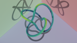
Figure 1: Magnetic streamlines for the twisted trefoil knot with helicity at time $0$.

Apart from the class of knots described in equation (1) we also study one that requires a different description, the $8_{18}$ knot. Its central spine is given as

$$\bm{x}(s)=\left(\begin{array}[]{c}(C+\sin(4s))\sin(3s)\\ (C+\sin(4s))\cos(3s)\\ D\cos(8s)\end{array}\right),$$ (3)

with the same parameters as in equation (1). A rendering of the $8_{18}$ knot can be seen in Figure 6 (panel a) .

Apart from knots we also investigate the relaxation of links that are topologically non-trivial. One of them is the Borromean rings configuration. Unlike in its usual depiction, we do not project it onto a plane and choose a more symmetric representation consisting of three magnetic flux ovals. Those are arranged such that by removing one, the remaining two constitute two unlinked and topologically trivial flux rings. A rendering of the Borromean rings can be seen in Figure 5.

The last configuration consists of one flux ring that is linked with two others on opposing sides, like a short chain where the flux rings are the links. We can think of this configuration as a sort of double Hopf link where each of the two links contribute to the magnetic helicity content. By changing the sign of the flux in one of the outer rings we can construct topologically different cases, one with helicity and one without. A rendering of the triple ring configurations rings can be seen in Figure 3.

Since our computational code uses the magnetic vector potential $\bm{A}$ instead of the magnetic field $\bm{B}=\mbox{\boldmath$\nabla$}{}\times\bm{A}$ for the computation, we need as last step of the construction to compute the inverse curl. We can do this by first taking the curl

$$\bm{J}=\mbox{\boldmath$\nabla$}{}\times\bm{B},$$ (4)

which gives us the current density $\bm{J}$. We then express the current density using the magnetic vector potential as

$$\bm{J} = \mbox{\boldmath$\nabla$}{}\times\mbox{\boldmath$\nabla$}{}\times\bm{A}$$ (5)

$$= -\Delta\bm{A}+\mbox{\boldmath$\nabla$}{}(\mbox{\boldmath$\nabla$}{}\cdot\bm{A}).$$

Using the Coulomb gauge $\mbox{\boldmath$\nabla$}{}\cdot\bm{A}=0$ we can then perform a Fourier transform on the problem

$${\cal F}\{\bm{J}\}(\bm{k})=-k^{2}{\cal F}\{\bm{A}\}(\bm{k}),$$ (6)

invert it in $k$-space

$${\cal F}\{\bm{A}\}(\bm{k})=-{\cal F}\{\bm{J}\}(\bm{k})/k^{2},$$ (7)

solve this algebraic equation and transform this solution back into real space. Since all of our initial conditions are $0$ at the domain boundaries we have periodic initial conditions and the Fourier method leads to valid initial vector potentials $\bm{A}$, such that $\mbox{\boldmath$\nabla$}{}\times\bm{A}$ matches our initial construction of $\bm{B}$, up to small numerical errors.

II.2 Simulation Setup

The magnetic knot or link is the initial condition of our numerical experiments. We place the configuration into a Cartesian box with size $[8,8,8]$. Being periodic, there are no fluxes outside the domain.

In our model we make use of the magnetohydrodynamics equations of a viscous, diffusive, compressible gas

$$\frac{\partial\bm{A}}{\partial t} = \bm{u}\times\bm{B}+\eta\mbox{\boldmath$\nabla$}{}^{2}\bm{A},$$ (8)

$$\frac{{\rm D}{}\bm{u}}{{\rm D}{}t} = -c_{\rm s}^{2}\mbox{\boldmath$\nabla$}{}\ln{\rho}+\frac{\bm{J}\times\bm{B}}{\rho}+\bm{F}_{\rm visc},$$ (9)

$$\frac{{\rm D}{}\ln{\rho}}{{\rm D}{}t} = -\mbox{\boldmath$\nabla$}{}\cdot\bm{u},$$ (10)

with the fluid velocity $\bm{u}$, constant magnetic resistivity (diffusivity) $\eta$, advective derivative ${\rm D}{}/{\rm D}{}t=\partial/\partial t+\bm{u}\cdot\mbox{\boldmath$\nabla$}{}$, sound speed $c_{\rm s}=\gamma p/\rho$, density $\rho$, electric current density $\bm{J}=\mbox{\boldmath$\nabla$}{}\times\bm{B}$ and viscous force $\bm{F}_{\rm visc}$. The viscous force captures the friction between molecules and is given as $\bm{F}_{\rm visc}=\rho^{-1}\mbox{\boldmath$\nabla$}{}\cdot 2\nu\rho\mbox{\boldmath${\sf S}$}{}$, with the traceless rate of strain tensor $S_{ij}=\frac{1}{2}(u_{i,j}+u_{j,i})-\frac{1}{3}\delta_{ij}\mbox{\boldmath$\nabla$}{}\cdot\bm{u}$. We make implicitly use of an equation of state of an ideal monatomic gas, as we eliminated pressure $p$ for density $\rho$. To solve the equations we make use of the PencilCode Brandenburg-2020-Zenodo ; PencilCodeCollaboration-2021-58-2807-JOpSoSoft (https://github.com/pencil-code), which is a sixth order in space and fourth order in time finite difference code.

To keep kinetic and magnetic dissipation low we choose for the viscosity and magnetic resistivity $\nu=\eta=10^{-3}$ for most of our simulations. That way, the magnetic helicity won’t be significantly affected by magnetic diffusion during dynamically relevant times. In a comparison we will also show a few simulations using $\nu=\eta=5\times 10^{-4}$.

For the boundary conditions we choose periodic boundaries for all of our setups. Not only is this a computationally unproblematic condition, but it helps us conserving energy (magnetic and kinetic) and magnetic helicity together with current helicity.

II.3 Magnetic Helicity Dissipation

In an ideal fluid with no viscosity and no magnetic diffusion ($\nu=\eta=0$) the magnetic helicity

$$H_{\rm m}=\int_{V}\bm{A}\cdot\bm{B}\ {\rm d}{}V$$ (11)

is exactly conserved. $\nu$ and $\eta$ are finite, albeit very small, for physically interesting objects, like stars, galaxies, planetary interiors and fusion devices. From the MHD equations (8)–(10) we can easily derive the rate of change of the magnetic helicity as

$$\frac{\partial H_{\rm m}}{\partial t}=-2\eta\int_{V}\bm{J}\cdot\bm{B}\ {\rm d}{}V.$$ (12)

Here we see that for $\eta=0$ magnetic helicity is conserved. For a finite $\eta$ the rate of dissipation depends on the magnetic field strength, the current density and their alignment. In turbulent media the current can reach relatively high values as the magnetic field undergoes repeated reconnection events. So, even with a small $\eta$ we cannot exclude a significant change in the magnetic helicity content. Due to its importance in helicity conservation, we will monitor this value for our simulations.

III Results

III.1 Geometry Evolution

Before analyzing the evolution of the magnetic field and helicity in time we study the geometric evolution of the field lines. For the visualization of the magnetic streamlines we make use of the open-source tool BlenDaViz and trace a number of magnetic streamlines. The streamlines have their seeds where the field strength is relatively strong, so we avoid noise generated in weak field domains. Here we compare the topological structure of a selection of magnetic fields at their initial configuration and final state when we stop the calculations.

For all of our calculations we observe a fast dynamical regime until a simulation time of less than $100$. This regime is dominated by the Lorentz force that causes some of the configurations to contract. As the flux tubes approach, large currents are being generated which then leads to energy loss through Ohmic heating. After this regime, the resulting magnetic field is subject to a slow diffusion of time scale of $2000$ code time units.

III.1.1 Knots

In Figure 2 we show the initial field configuration for the trefoil knots together with the final field configurations after magnetic relaxation. For a fair comparison the final time is $t=150$ in code units for all configurations. The internal twist is ascending from left to right and is chosen such that the second knot (panels b and e) has a twist that generates a helicity exactly opposite of the helicity from the knotedness. The highly twisted knot has a helicity of equal strength, but opposite sign of the untwisted knot (panels c and f) .

From the magnetic helicity conservation and the realizability condition we would expect that after relaxation, and the accompanying field line reconnection, the two helical cases (a and c) should approximately stay helical while the non-helical case should lose all its initial structure. However, all three configurations clearly show a twist and with that a helical field at final times. This is on contrast to previous findings where non-helical fields would evolve into a state with no discernible structure fluxRings10 . This is clearly due to a generation of magnetic helicity within dynamical time scales, as we will discuss in more detail further below. This helicity generation is clearly not strong enough for the untwisted knot to be transformed into a non-helical field, which would then lose its initial structure. But it is fast enough for the twisted knot to generate a large enough amount of helicity, in a time much shorter than the diffusive time, so that the final structure is similarly twisted as the plain knot.

\begin{overpic}[width=281.85034pt]{n3_r256_tw0_t0} \put(5.0,5.0){\large\lx@texthl@color{a) $t=0$, tw$=0$}} \end{overpic}

\begin{overpic}[width=281.85034pt]{n3_r256_tw061009_t0} \put(5.0,5.0){\large\lx@texthl@color{b) $t=0$, tw$=1$}} \end{overpic}

\begin{overpic}[width=281.85034pt]{n3_r256_tw1_219755_t0} \put(5.0,5.0){\large\lx@texthl@color{c) $t=0$, tw$=2$}} \end{overpic}

\begin{overpic}[width=281.85034pt]{n3_r256_tw0_tf} \put(5.0,5.0){\large\lx@texthl@color{d) $t=150$, tw$=0$}} \end{overpic}

\begin{overpic}[width=281.85034pt]{n3_r256_tw061009_tf} \put(5.0,5.0){\large\lx@texthl@color{e) $t=150$, tw$=1$}} \end{overpic}

\begin{overpic}[width=281.85034pt]{n3_r256_tw1_219755_tf} \put(5.0,5.0){\large\lx@texthl@color{f) $t=150$, tw$=2$}} \end{overpic}

Figure 2: Initial magnetic streamlines for the trefoil knot configuration (top) using different twist parameter ${\rm tw}$ such that the left has no twist, the middle has a twist that reduces the helicity to zero and the right a strong twist with opposite helicity to the left one. The lower figures show the streamlines at time $150$.

For the $4$-foil and $5$-foil knot configurations we observe qualitatively the same behaviour. Since the initial helicity is larger than for the trefoil knot the final state is more twisted. For the non-helical case with the opposing internal twist, we observe a significant generation of twist and therefore helicity. To conserve space we moved the results for the $4$-foil and $5$-foil knots to appendix A.

III.1.2 Triple Rings

For the triple rings configurations we have five realizations divided into two sets. One set derives from the non-helical configuration and the other form the helical. By adding an internal twist to the non-helical we can induce a magnetic helicity content of the same size as the untwisted helical triple ring. For the helical triple rings we can add a twist so that the helicity exactly vanishes and an opposite twist to double the magnetic helicity compared to the untwisted case.

The three linked rings, by contrast to the knots, do not show much unexpected behaviour. Here, the helical configurations retain their topological structure during the relaxation, while the non-helical ones decay into a field that is more trivial (see Figure 3 and Figure 4). Unlike the twisted non-helical knots, the twisted non-helical triple ring field (Figure 4, panels a and c) does not show any significant generation of helicity. With that the relaxed field is roughly trivial.

\begin{overpic}[width=281.85034pt]{linked_tori_h0_r256_tw0_t0} \put(5.0,5.0){\large\lx@texthl@color{a) $t=0$, tw$=0$, $H_{0}=0$}} \end{overpic}

\begin{overpic}[width=281.85034pt]{linked_tori_h0_r256_tw0_271_t0} \put(5.0,5.0){\large\lx@texthl@color{b) $t=0$, tw$=1$, $H_{0}=0$}} \end{overpic}

\begin{overpic}[width=281.85034pt]{linked_tori_h0_r256_tw0_tf} \put(5.0,5.0){\large\lx@texthl@color{c) $t=150$, tw$=0$, $H_{0}=0$}} \end{overpic}

\begin{overpic}[width=281.85034pt]{linked_tori_h0_r256_tw0_271_tf} \put(5.0,5.0){\large\lx@texthl@color{d) $t=150$, tw$=1$, $H_{0}=0$}} \end{overpic}

Figure 3: Initial magnetic streamlines for the triple ring configurations (top). With twist parameter ${\rm tw}=0$ this would be a non-helical field (hence $H_{0}=0$) . The lower figures show the streamlines at time $150$.

\begin{overpic}[width=281.85034pt]{linked_tori_h2_r256_tw-0_271_t0} \put(5.0,5.0){\large\lx@texthl@color{a) $t=0$, tw$=-1$, $H_{0}=2$}} \end{overpic}

\begin{overpic}[width=281.85034pt]{linked_tori_h2_r256_tw0_t0} \put(5.0,5.0){\large\lx@texthl@color{b) $t=0$, tw$=0$, $H_{0}=2$}} \end{overpic}

\begin{overpic}[width=281.85034pt]{linked_tori_h2_r256_tw0_271_t0} \put(5.0,5.0){\large\lx@texthl@color{c) $t=0$, tw$=1$, $H_{0}=2$}} \end{overpic}

\begin{overpic}[width=281.85034pt]{linked_tori_h2_r256_tw-0_271_tf} \put(5.0,5.0){\large\lx@texthl@color{d) $t=150$, tw$=-1$, $H_{0}=2$}} \end{overpic}

\begin{overpic}[width=281.85034pt]{linked_tori_h2_r256_tw0_tf} \put(5.0,5.0){\large\lx@texthl@color{e) $t=150$, tw$=0$, $H_{0}=2$}} \end{overpic}

\begin{overpic}[width=281.85034pt]{linked_tori_h2_r256_tw0_271_tf} \put(5.0,5.0){\large\lx@texthl@color{f) $t=150$, tw$=1$, $H_{0}=2$}} \end{overpic}

Figure 4: Initial magnetic streamlines for the triple ring configurations (top). With twist parameter ${\rm tw}=0$ this would be a helical field (hence $H_{0}=2$) . The left field has negative twist parameter and the right one positive. With the amount of negative twist the magnetic helicity of the left configuration is zero and the helicity of the right configuration is double to the untwisted case. The lower figures show the streamlines at time $150$.

We attribute this different behavior to the absence of any significant magnetic helicity generation from the internal twist. Currently we cannot explain why this is the case for the other test configurations, but not for the triple rings configuration.

III.1.3 Borromean Rings

For the untwisted Borromean rings we observe the same behaviour as in the work by knotsDecay11, . This is not surprising, as the simulation setup is very close to theirs and we make use of the same numerical code. Here we see that the non-helical Borromean rings undergo a series of reconnection events and relax into a configuration consisting of two separate and oppositely twisted fields (Figure 5, panel c).

The Borromean rings configuration with the internal twist, however, relaxes into a relatively compact field (panel d) . This field has a clear twist, which is a consequence of the magnetic helicity conservation in this low resistivity system. Like the triple-ring, and in contrast to the knots, we observe a behavior predicted from the magnetic helicity conservation.

\begin{overpic}[width=281.85034pt]{borromean_r256_tw0_t0} \put(5.0,5.0){\large\lx@texthl@color{a) $t=0$, tw$=0$}} \end{overpic}

\begin{overpic}[width=281.85034pt]{borromean_r256_tw0_0351_t0} \put(5.0,5.0){\large\lx@texthl@color{b) $t=0$, tw$=1$}} \end{overpic}

\begin{overpic}[width=281.85034pt]{borromean_r256_tw0_tf} \put(5.0,5.0){\large\lx@texthl@color{c) $t=150$, tw$=0$}} \end{overpic}

\begin{overpic}[width=281.85034pt]{borromean_r256_tw0_0351_tf} \put(5.0,5.0){\large\lx@texthl@color{d) $t=150$, tw$=1$}} \end{overpic}

Figure 5: Initial magnetic streamlines for the Borromean rings configurations (top) with (left) and without (right) internal twist. The lower figures show the streamlines at time $150$. Note the slightly changed perspective compared to the other streamline plots.

III.1.4 $8_{18}$ Knot

The plain $8_{18}$ knot is a non-helical configuration. With helicity conservation we expect a topologically trivial relaxed field at final simulation time. Although we indeed do not observe any significant change in magnetic helicity the final state appears to be a topologically non-trivial bundle of twisted field lines (Figure 6 panel c). However, upon closer inspection, we see that this bundle has only a small net twist, which makes it topologically trivial.

The twisted $8_{18}$ knot is a helical field with its helicity coming entirely from the twist. If its magnetic helicity is approximately conserved during its relaxation, we should see a topologically non-trivial field at the end of the simulation. This is indeed what we observe in panel d, where there is a clear twist at the final time.

\begin{overpic}[width=281.85034pt]{iucaa_r256_tw0_t0} \put(5.0,5.0){\large\lx@texthl@color{a) $t=0$, tw$=0$}} \end{overpic}

\begin{overpic}[width=281.85034pt]{iucaa_r256_tw-4_t0} \put(5.0,5.0){\large\lx@texthl@color{b) $t=0$, tw$=-1$}} \end{overpic}

\begin{overpic}[width=281.85034pt]{iucaa_r256_tw0_tf} \put(5.0,5.0){\large\lx@texthl@color{c) $t=150$, tw$=0$}} \end{overpic}

\begin{overpic}[width=281.85034pt]{iucaa_r256_tw-4_tf} \put(5.0,5.0){\large\lx@texthl@color{d) $t=150$, tw$=-1$}} \end{overpic}

Figure 6: Initial magnetic streamlines for the $8_{18}$ knot configurations (top) with and without internal twist. The lower figures show the streamlines at time $150$.

III.2 Magnetic Helicity

In the limit of vanishing magnetic resistivity, we know that the magnetic helicity is conserved (see equation (12)). However, this is only true if the $\bm{J}\cdot\bm{B}$ term is not so large as to compensate for a small $\eta$. If there is a net alignment between the magnetic field $\bm{B}$ and electric current density $\bm{J}$ then we should see dissipation. For a net anti-alignment we would observe an increase in helicity. Potential loci for this to happen are reconnection regions, since there $\bm{J}$ and $\bm{B}$ are relatively aligned. Furthermore, the current in these regions typically increases significantly which leads to Ohmic heating.

Other sources of $\bm{J}$–$\bm{B}$ alignment are magnetic twist. For an untwisted magnetic flux tube the generating currents are purely toroidal. Adding a twist has two effects. First, the toroidal magnetic field component is now aligned with the toroidal current that generates the untwisted part of the magnetic field. Second, the twist component is generated by an axial magnetic field and is aligned with the axial magnetic field of the untwisted magnetic field component.

To better understand the helicity evolution for our simulations we monitor the volume averaged magnetic helicity in time. The definition of this average is

$$\langle\bm{A}\cdot\bm{B}\rangle=\frac{1}{V}\int_{V}\bm{A}\cdot\bm{B}\ {\rm d}{}V.$$ (13)

Since we are also interested in the generation of helicity we also monitor the spatially averaged current helicity

$$\langle\bm{J}\cdot\bm{B}\rangle=\frac{1}{V}\int_{V}\bm{J}\cdot\bm{B}\ {\rm d}{}V.$$ (14)

III.2.1 Knots

For the untwisted knots we observe a relatively slow loss of helicity (Figure 7, solid lines). While the initial loss is fast, after some short time it slows down. Nevertheless, the loss is faster than the expected resistive decay time of $\tau_{\rm res}=L^{2}/\eta\approx 1000$, where $L\approx 1$ is a typical length scale of the system. So we already see that even without internal twist, the contribution of the $\bm{J}$–$\bm{B}$-alignment is significant.

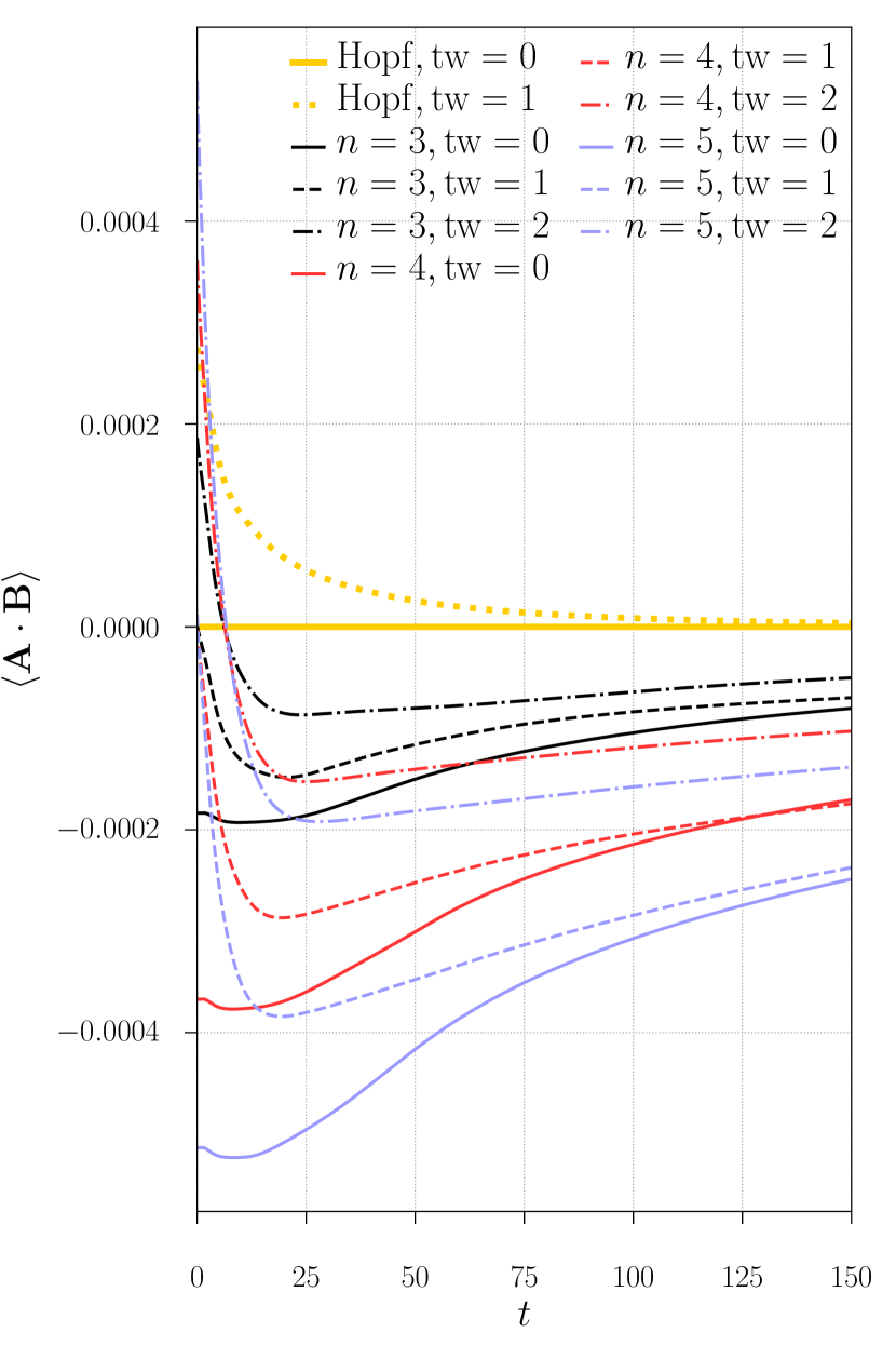
Figure 7: Mean magnetic helicity in dependence of time for the knot configurations and the Hop link using different twist parameters ${\rm tw}$.

For the twisted knots with zero helicity (Figure 7, dashed lines) we see a significant generation of negative helicity at initial times. The time scales are much shorter than the diffusion time. This change is again due to the net alignment of $\bm{J}$ and $\bm{B}$, which is even more significant than for the untwisted knots.

For the highly twisted knots with opposite magnetic helicity we see a strong initial decrease of helicity. Similar to the previous cases, this is due to an even stronger alignment of $\bm{J}$ and $\bm{B}$. Within this very short time period we even observe a sign change and an approach to the magnetic helicity of the untwisted case.

The $\bm{J}\cdot\bm{B}$ term is so dominant, that within much less than the diffusion time we see a significant decrease in magnetic helicity for the twisted cases. This effect is increases with twist parameter (see Figure 8).

For comparison we also plot the Hopf link in the same graph. This configuration is helical due to the mutual linking of two magnetic flux rings. Similarly to the knots we can add an internal twist to the magnetic flux tubes to reduce the helicity content to $0$. Unlike the twisted knots with zero initial helicity, the twisted Hopf link with no initial helicity does not show any significant change within dynamical times. This shows that a twist does not necessarily lead to a $\bm{J}$–$\bm{B}$ alignment.

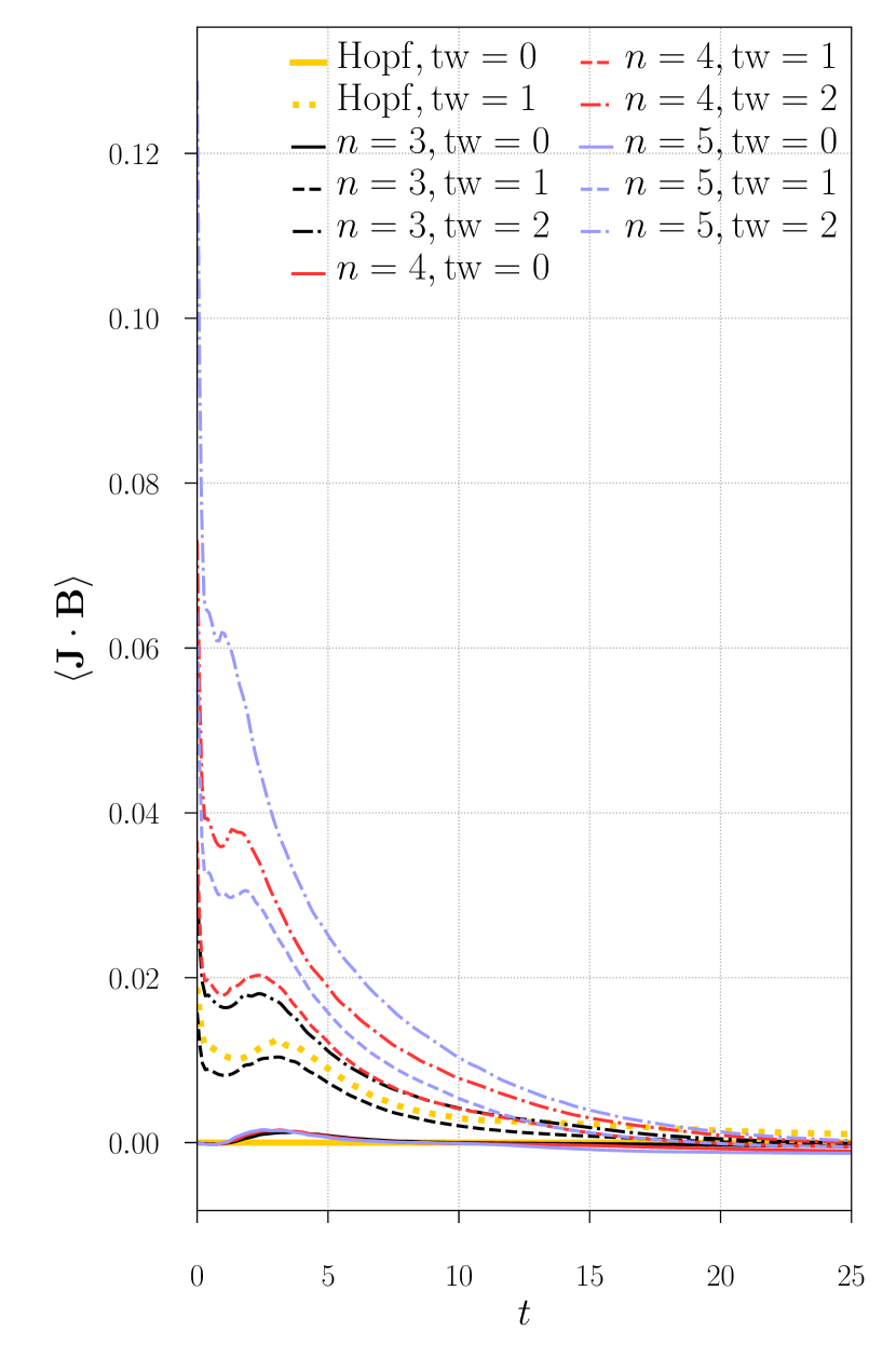
Figure 8: Mean current helicity in dependence of time for the knot configurations and the Hop link using different twist parameters ${\rm tw}$.

III.2.2 Triple Rings

While the twisted knots showed a significant change in magnetic helicity at time scales much shorter than the diffusive time, the twisted triple ring configurations exhibit a less dramatic behavior (see Figure 9). This behavior is more reminiscent of what we would expect if we assumed that helicity was conserved due to the small magnetic diffusivity $\eta$. The reason is a much weaker alignment of the current density and the magnetic field, even for the case of a strong internal twist. Although currently we cannot give an explanation on why the triple rings behave differently, it shows that an internal twist does not necessarily lead to helicity decay or generation.

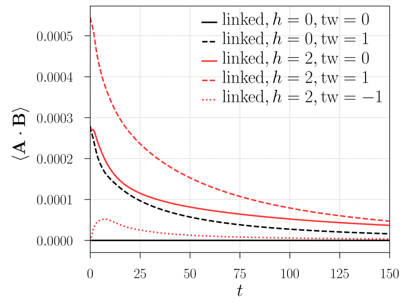
Figure 9: Mean magnetic helicity in dependence of time for the linked triple rings configurations using different twist parameter ${\rm tw}$. Cases labeled as $h=0$ are the triple rings with no helicity if the twist was zero. Those labeled $h=2$ are the ones with helicity if the twist was zero.

III.2.3 Borromean Rings and $8_{18}$ Knot

The twisted Borromean rings and the $8_{18}$ knot both show similar decay rates for the magnetic helicity (Figure 10). Within time scales as short as ca. $1\%$ of the diffusive time scale the helicity already dissipates. This should be contrasted to the near conservation for the case of no internal twist.

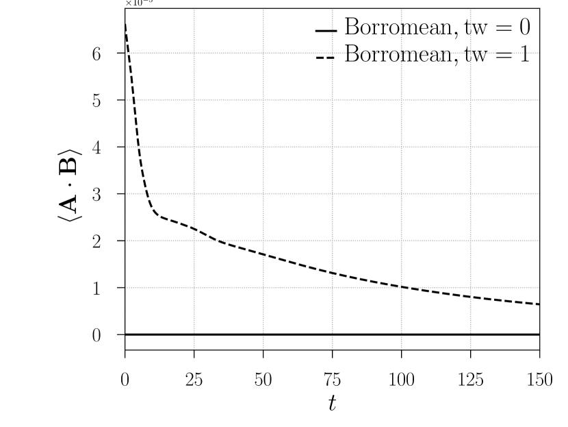
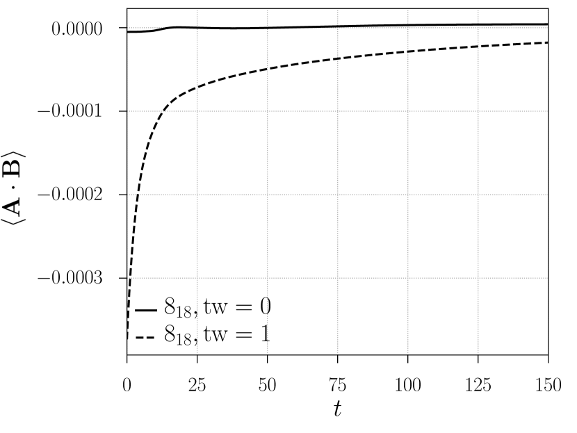
Figure 10: Mean magnetic helicity in dependence of time for the Borromean rings (upper panel) and $8_{18}$ knot (lower panel) configurations using different twist parameter ${\rm tw}$.

The different behavior of the twist and no-twist case can be explained by the alignment of $\bm{J}$ and $\bm{B}$. From Figure 11 we see that the untwisted Borromean rings and untwisted $8_{18}$ knot have a constantly low helicity production term. This contrasts to the much larger values for the twisted cases. So, similarly to the knots, the internal twist leads to helicity decay due to a significant alignment of $\bm{J}$ and $\bm{B}$.

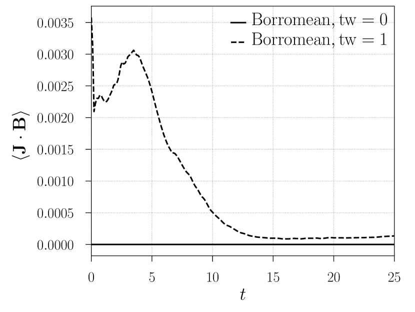
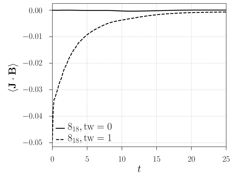
Figure 11: Mean current helicity in dependence of time for the Borromean rings (upper panel) and $8_{18}$ knot (lower panel) configurations using different twist parameter ${\rm tw}$.

III.3 Magnetic Energy

From previous studies fluxRings10 ; knotsDecay11 we know that magnetic knots and links have a slow energy decay compared to topologically trivial configurations. It has been shown that, rather than the actual linking, the magnetic helicity content is the determining factor for the speed of energy decay fluxRings10 .

Here we have a set of test cases that can either corroborate those findings or put a caveat to them. If the magnetic helicity alone was the determining factor, then for the helical cases we should see a slow decay while for the twisted zero-helicity cases we should see a faster energy decay.

To test this hypothesis we plot the spatially averaged magnetic energy density for the triple ring configurations with and without twist (Figure 12) and then normalize to its initial value ar $t=0$. This spatial average is analogous to what we did for the helicities, i.e.

$$\langle\bm{B}^{2}\rangle=\frac{1}{V}\int_{V}\bm{B}^{2}\ {\rm d}{}V.$$ (15)

There we see that it is indeed the magnetic helicity that determines the speed of the energy decay. For the two non-helical configurations there is a steeper decay than for the three helical cases.

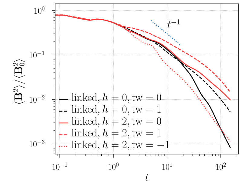
Figure 12: Normalized magnetic energy in dependence of time for the triple rings configurations using different twist parameter ${\rm tw}$. For guidance we add a power law of $t^{-1}$.

Of course we could have just picked the set of test cases that exactly proved our hypothesis. So, we also plot the magnetic energy for the knots (Figure 13). There we can clearly see that the energy decay is of the same speed for all test cases, independent of the type of knot (3, 4 or 5-foil) and the internal twist ${\rm tw}$. Unlike the previous studies this suggests that it is the field line topology manifested as knottedness and twist that is more of a determinant than the initial helicity itself. Here we emphasize initial, as the helicity can rapidly change even in our low resistivity environment, as we have seen in the previous section. This non-conservation is the reason for the similar energy decay.

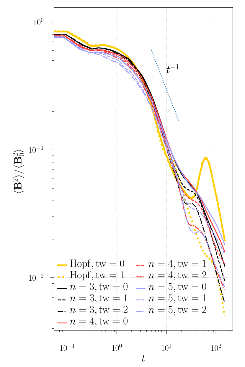
Figure 13: Normalized magnetic energy in dependence of time for the knot configurations using different twist parameter ${\rm tw}$. For guidance we add a power law of $t^{-1}$.

Since for the Borromean rings and the $8_{18}$ knot we also observe a rapid loss of magnetic helicity we would expect that the helical and non-helical cases exhibit a similar decay rate for the magnetic energy. From Figure 14 we see that this is indeed the case. The decay rates are almost indistinguishable.

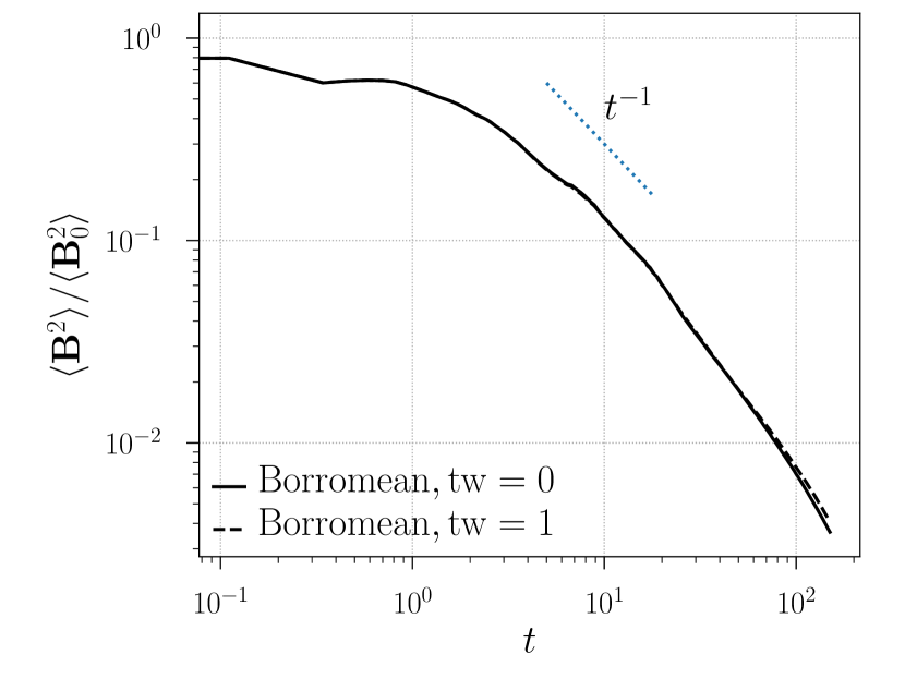
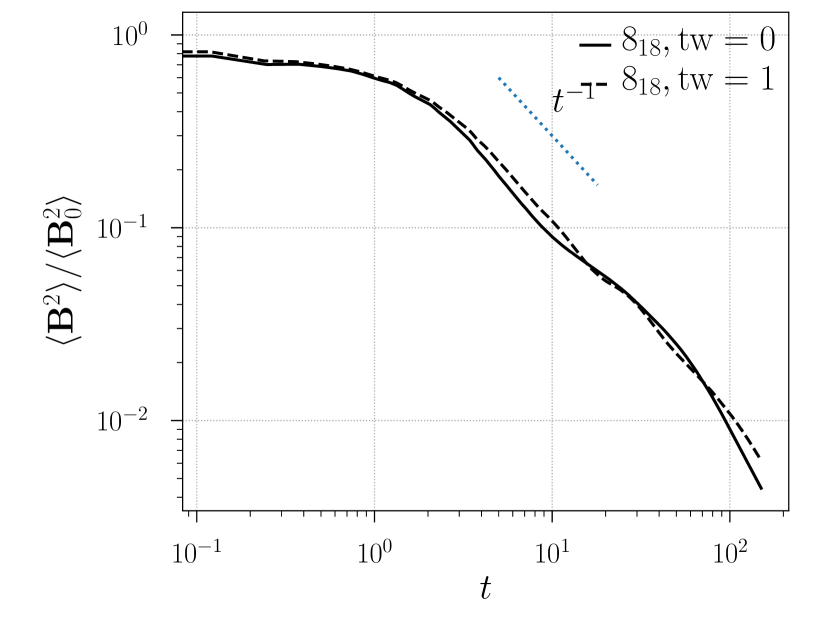
Figure 14: Normalized magnetic energy in dependence of time for the Borromean rings configurations (top panel) and $8_{18}$ knot (bottom panel) using different twist parameter ${\rm tw}$. For guidance we add a power law of $t^{-1}$.

While the realizability condition provides a lower bound of the magnetic energy in presence of magnetic helicity, an initially helical field is no guarantee that the energy decays only slowly. The observed helicity losses at time scales much shorter than the diffusive time annul such decay restrictions. We saw that only for the triple rings there is a relative conservation of helicity and with that a slow energy decay.

IV Effect of Low Magnetic Resistivity

The $\bm{J}\cdot\bm{B}$-term that is responsible for the generation and annihilation of magnetic helicity, is clearly large enough to lead to significant changes in the helicity within dynamical time scales. Since we have a prefactor of the magnetic resistivity $\eta$ in equation (12) we expect an insignificant change in helicity in low resistivity systems, like the solar atmosphere or laboratory plasmas.

At the same time we know that with reduced resistivity, plasmas are more turbulent and magnetic reconnection is more efficient. For reconnection to happen we need alignment of $\bm{J}$ and $\bm{B}$. So, it is conceivable that in the low resistivity regime a reduced $\eta$ is compensated by an increased $\bm{J}\cdot\bm{B}$.

In this section we like to study the rate of change of magnetic helicity for low dissipation regimes. We repeat the numerical experiment for the trefoil knot with strong internal twist, i.e. with internal twist that changes the sign of the magnetic helicity. We halve the magnetic resistivity $\eta$ to $5\times 10^{-4}$, as well as the viscosity $\nu$ to $5\times 10^{-4}$ in order to keep the Prandtl number at $1$.

We first observe that the alignment of the electric current density $\bm{J}$ and the magnetic field $\bm{B}$ is stronger with reduced magnetic diffusion (see Figure 15). At early times (until ca. $t=5$) the difference is relatively small by ca. $30\%$. At later times, the relative difference is more of a factor of $4$, where $\bm{J}\cdot\bm{B}$ is small for both cases. For the helicity production this quantity is relevant, but also carries a prefactor of $\eta$, which is half for the low diffusion case.

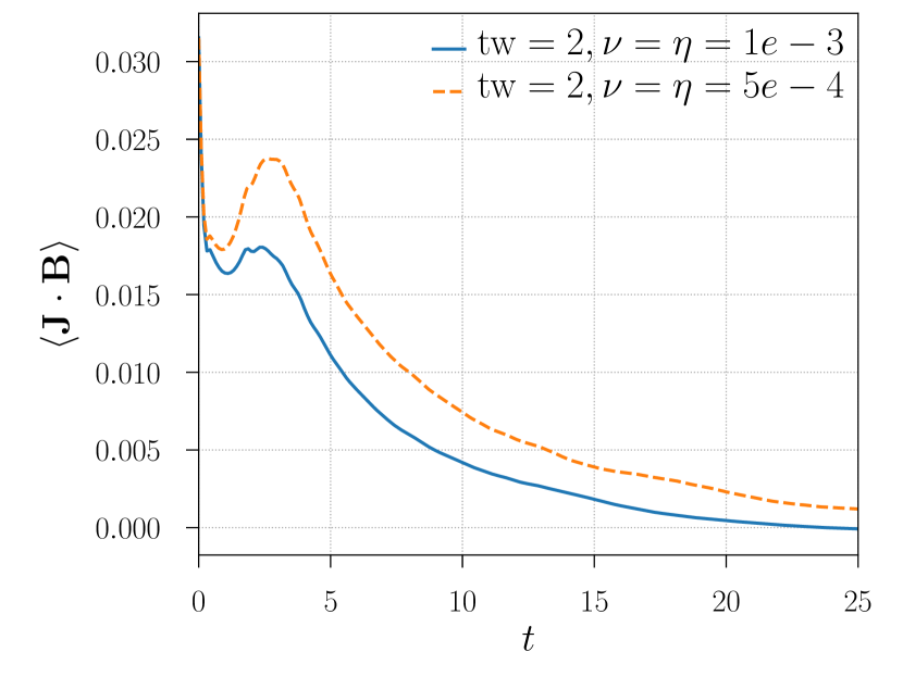
Figure 15: Alignment of the electric current density $\bm{J}$ and magnetic field $\bm{B}$ for the trefoil knot with twist $2$ and comparing high and low diffusivity.

The observed increase of the $\bm{J}$–$\bm{B}$ alignment is, however, not strong enough to compensate for the halved prefactor $\eta$ in the helicity production. For the helicity we observe a significantly smaller drop for the low diffusion case (see Figure 16). From the realizability condition, we would therefore expect a smaller drop in magnetic energy, at least for those times. This is indeed what we observe (see Figure 17). However, for later times there is a drop in magnetic helicity even for the low diffusion case, which is why we also observe a significant drop in magnetic energy at time $t>40$.

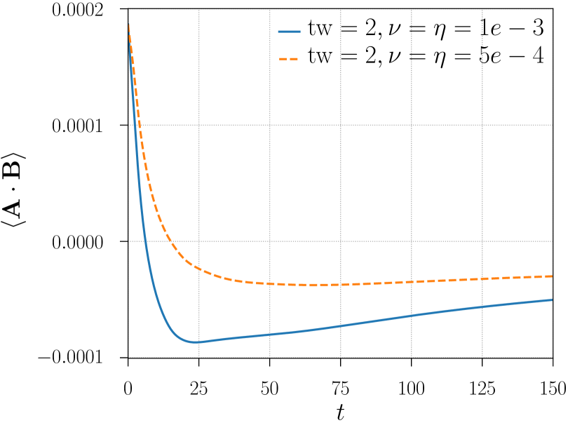
Figure 16: Mean magnetic helicity in dependence of time for the trefoil knot with twist $2$ and comparing high and low diffusivity.

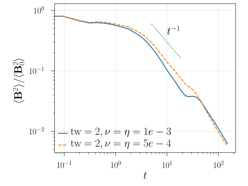
Figure 17: Normalized magnetic energy in dependence of time for the trefoil knot with twist $2$ and comparing high and low diffusivity.

V Conclusions

In our study we investigated the the robustness of the role of magnetic helicity in the relaxation of topologically non-trivial magnetic flux tubes in a plasma environment. This was done by simulating the visco-resistive relaxation of magnetic knots and links. To contrast the effect of topology and magnetic helicity we vary the internal twist of the fields.

While we confirm the importance of the realizability condition as restriction of the field relaxation, the presence of magnetic helicity does not automatically lead to a restricted decay. One reason for this is the presence of source terms for the magnetic helicity. Especially for fields with an internal twist we see that this term can be so large to significantly change the helicity content within dynamical time scales. With the loss of helicity, the restrictions on the relaxation do not hold.

This has implications for solar magnetic fields, as they show topologically non-trivial forms and can contain an internal twist. Here we should keep in mind that through the twist the alignment of the magnetic field with the electric current density is significant and can potentially lead to changes in helicity. However, to draw more precise conclusions for solar magnetic fields, either in the convection zone, chromosphere or corona, we would require a study that incorporates parameters found in such environments, such as density and temperature gradients.

In order to apply our findings to laboratory or stellar plasmas we also need to consider the scaling of all of our terms, particularly the $\bm{J}$–$\bm{B}$ alignment. If we were to reduce the scale of our systems while keeping the magnetic field strength $\bm{B}$ constant, our currents $\bm{J}$ would increase due to the larger spatial variations. The same argument can be applied to the magnetic vector potential $\bm{A}$ which would decrease in strength. The result is a smaller magnetic helicity density $h=\bm{A}\cdot\bm{B}$ and a larger $\bm{J}$–$\bm{B}$ alignment. The increased $\bm{J}$–$\bm{B}$ alignment leads to an increased loss/generation rate of magnetic helicity that is inversely proportional to the scaling. So, a half size system would lose/generate the same amount of helicity in half the time.

However, if we ask about the loss of normalized (to time $0$) helicity we introduce one more scaling by dividing by the initial magnetic helicity. The loss of this quantity happens then on a quarter of the time of the un-scaled system. Furthermore, in turbulent scenarios it is usually the resistive time scale that is important, which is $\tau_{\rm res}=L^{2}/\eta$. With changing scale $L$ our normalized magnetic helicity would then change at the same diffusive times as in the un-scaled system.

Author Declarations

Conflict of Interest

The authors have no conflicts to disclose.

Author Contributions

Simon Candelaresi: Conceptualization (lead); Data curation (lead); Formal analysis (lead); Investigation (lead); Methodology (lead); Visualization (lead); Writing – original draft (lead). Software (supporting); Validation (supporting); Celine Beck: Software (lead); Validation (lead); Investigation (supporting); Methodology (supporting); Formal analysis (supporting); Writing – original draft (supporting).

Data Availability Statement

The data that support the findings of this study are available from the corresponding author upon reasonable request.

Appendix A Field Evolution

For completeness we show the evolution of the knots that have been mentioned only in passing. Those are the $4$ and $5$-foil knots. The qualitative evolution is the same as for the trefoil knot (see Figure 18 and Figure 19) with the appearance of a twisted structure even for the initially non-helical case.

\begin{overpic}[width=281.85034pt]{n4_r256_tw0_t0} \put(5.0,5.0){\large\lx@texthl@color{a) $t=0$, tw$=0$}} \end{overpic}

\begin{overpic}[width=281.85034pt]{n4_r256_tw1_041975_t0} \put(5.0,5.0){\large\lx@texthl@color{b) $t=0$, tw$=1$}} \end{overpic}

\begin{overpic}[width=281.85034pt]{n4_r256_tw2_08283_t0} \put(5.0,5.0){\large\lx@texthl@color{c) $t=0$, tw$=2$}} \end{overpic}

\begin{overpic}[width=281.85034pt]{n4_r256_tw0_tf} \put(5.0,5.0){\large\lx@texthl@color{d) $t=150$, tw$=0$}} \end{overpic}

\begin{overpic}[width=281.85034pt]{n4_r256_tw1_041975_tf} \put(5.0,5.0){\large\lx@texthl@color{e) $t=150$, tw$=1$}} \end{overpic}

\begin{overpic}[width=281.85034pt]{n4_r256_tw2_08283_tf} \put(5.0,5.0){\large\lx@texthl@color{f) $t=150$, tw$=2$}} \end{overpic}

Figure 18: Initial magnetic streamlines for the $4$-foil knot configuration (top) using different twist parameter ${\rm tw}$ such that the left has no twist, the middle has a twist that reduces the helicity to zero and the right a strong twist with opposite helicity to the left one. The lower figures show the streamlines at time $150$.

\begin{overpic}[width=281.85034pt]{n5_r256_tw0_t0} \put(5.0,5.0){\large\lx@texthl@color{a) $t=0$, tw$=0$}} \end{overpic}

\begin{overpic}[width=281.85034pt]{n5_r256_tw1_497275_t0} \put(5.0,5.0){\large\lx@texthl@color{b) $t=0$, tw$=1$}} \end{overpic}

\begin{overpic}[width=281.85034pt]{n5_r256_tw2_99621_t0} \put(5.0,5.0){\large\lx@texthl@color{c) $t=0$, tw$=2$}} \end{overpic}

\begin{overpic}[width=281.85034pt]{n5_r256_tw0_tf} \put(5.0,5.0){\large\lx@texthl@color{d) $t=150$, tw$=0$}} \end{overpic}

\begin{overpic}[width=281.85034pt]{n5_r256_tw1_497275_tf} \put(5.0,5.0){\large\lx@texthl@color{e) $t=150$, tw$=1$}} \end{overpic}

\begin{overpic}[width=281.85034pt]{n5_r256_tw2_99621_tf} \put(5.0,5.0){\large\lx@texthl@color{f) $t=150$, tw$=2$}} \end{overpic}

Figure 19: Initial magnetic streamlines for the $5$-foil knot configuration (top) using different twist parameter ${\rm tw}$ such that the left has no twist, the middle has a twist that reduces the helicity to zero and the right a strong twist with opposite helicity to the left one. The lower figures show the streamlines at time $150$.

References

- (1) The Pencil Code, a modular MPI code for partial differential equations and particles: multipurpose and multiuser-maintained. Journal of Open Source Software, 6:2807, 2021. doi:10.21105/joss.02807.
- (2) P. M. Akhmet’ev. Quadratic helicities and the energy of magnetic fields. P. Steklov Inst. Math., 278:10–21, 2012. doi:10.1134/S0081543812060028.
- (3) P. M. Akhmetev, S. Candelaresi, and A. Y. Smirnov. Calculations for the practical applications of quadratic helicity in MHD. Phys. Plasmas, 24:102128, 2017. doi:10.1063/1.4996288.
- (4) P. M. Akhmetev, S. Candelaresi, and A. Y. Smirnov. Minimum quadratic helicity states. J. Plasma Phys., 84:775840601, 2018. doi:10.1017/S0022377818001095.
- (5) V. I. Arnold. The asymptotic Hopf invariant and its applications. Sel. Math. Sov., 5:327–345, 1986. doi:10.1007/978-3-642-31031-7_32.
- (6) G. Barnes. On the relationship between coronal magnetic null points and solar eruptive events. Astrophys. J. Lett., 670:L53, 2007. doi:10.1086/524107.
- (7) D. Biskamp. Magnetohydrodynamic Turbulence. Cambridge University Press, 2003. doi:10.1017/CBO9780511535222.
- (8) F. Boris. Observation of a 3d magnetic null point in the solar corona. Sol. Phys., 185:297–309, 1999. doi:10.1023/A:1005124915577.
- (9) A. Brandenburg. Scientific usage of the Pencil Code, July 2020. doi:10.5281/zenodo.3947506.
- (10) A. Brandenburg and K. Subramanian. Astrophysical magnetic fields and nonlinear dynamo theory. Phys. Rep., 417:1–209, 2005. doi:10.1016/j.physrep.2005.06.005.
- (11) S. Candelaresi and A. Brandenburg. Decay of helical and nonhelical magnetic knots. Phys. Rev. E, 84:016406, 2011. doi:10.1103/PhysRevE.84.016406.
- (12) S. Candelaresi and A. Brandenburg. Kinetic helicity needed to drive large-scale dynamos. Phys. Rev. E, 87:043104, 2013. doi:10.1103/PhysRevE.87.043104.
- (13) I. J. D. Craig and A. D. Sneyd. A dynamic relaxation technique for determining the structure and stability of coronal magnetic fields. Astrophys. J., 311:451–459, 1986. doi:10.1086/164785.
- (14) I. J. D. Craig and A. D. Sneyd. Nonlinear development of the kink instability in coronal flux tubes. Astrophys. J., 357:653–661, 1990. doi:10.1086/168954.
- (15) F. Del Sordo, S. Candelaresi, and A. Brandenburg. Magnetic-field decay of three interlocked flux rings with zero linking number. Phys. Rev. E, 81:036401, 2010. doi:10.1103/PhysRevE.81.036401.
- (16) U. Frisch, A. Pouquet, J. Léorat, and A. Mazure. Possibility of an inverse cascade of magnetic helicity in magnetohydrodynamic turbulence. J. Fluid Mech., 68:769–778, 1975.
- (17) J. D. Hunter. Matplotlib: A 2d graphics environment. Comput. Sci. Eng., 9:90–95, 2007. doi:10.1109/MCSE.2007.55.
- (18) J. C. Kasper, K. G. Klein, E. Lichko, Jia Huang, C. H. K. Chen, S. T. Badman, J. Bonnell, P. L. Whittlesey, R. Livi, D. Larson, M. Pulupa, A. Rahmati, D. Stansby, K. E. Korreck, M. Stevens, A. W. Case, S. D. Bale, M. Maksimovic, M. Moncuquet, K. Goetz, J. S. Halekas, D. Malaspina, Nour E. Raouafi, A. Szabo, R. MacDowall, Marco Velli, Thierry Dudok de Wit, and G. P. Zank. Parker solar probe enters the magnetically dominated solar corona. Phys. Rev. Lett., 127:255101, 2021. doi:10.1103/PhysRevLett.127.255101.
- (19) N. I. Kleeorin and A. A. Ruzmaikin. Dynamics of the average turbulent helicity in a magnetic field. Magnetohydrodynamics, 18:116, 1982.
- (20) F. Krause and K. H. Rädler. Dynamo theory of the Sun’s general magnetic fields on the basis of a mean-field magnetohydrodynamics. In R. Howard, editor, Solar Magnetic Fields, volume 43 of IAU Symposium, page 770, 1971. doi:10.1017/S0074180900023238.
- (21) H. K. Moffatt. Magnetic field generation in electrically conducting fluids. Camb. Univ. Press, 1978. doi:10.1017/S002211207923067X.
- (22) O. Motojima, K. Ida, K.Y. Watanabe, Y. Nagayama, A. Komori, T. Morisaki, B.J. Peterson, Y. Takeiri, K. Ohkubo, K. Tanaka, T. Shimozuma, S. Inagaki, T. Kobuchi, S. Sakakibara, J. Miyazawa, H. Yamada, N. Ohyabu, K. Narihara, K. Nishimura, M. Yoshinuma, S. Morita, T. Akiyama, N. Ashikawa, C.D. Beidler, M. Emoto, T. Fujita, T. Fukuda, H. Funaba, P. Goncharov, M. Goto, T. Ido, K. Ikeda, A. Isayama, M. Isobe, H. Igami, K. Ishii, K. Itoh, O. Kaneko, K. Kawahata, H. Kawazome, S. Kubo, R. Kumazawa, S. Masuzaki, K. Matsuoka, T. Minami, S. Murakami, S. Muto, T. Mutoh, Y. Nakamura, H. Nakanishi, Y. Narushima, M. Nishiura, A. Nishizawa, N. Noda, T. Notake, H. Nozato, S. Ohdachi, Y. Oka, S. Okajima, M. Osakabe, T. Ozaki, A. Sagara, T. Saida, K. Saito, M. Sakamoto, R. Sakamoto, Y. Sakamoto, M. Sasao, K. Sato, M. Sato, T. Seki, M. Shoji, S. Sudo, N. Takeuchi, H. Takenaga, N. Tamura, K. Toi, T. Tokuzawa, Y. Torii, K. Tsumori, T. Uda, A. Wakasa, T. Watari, I. Yamada, S. Yamamoto, K. Yamazaki, M. Yokoyama, and Y. Yoshimura. Overview of confinement and MHD stability in the Large Helical Device. Nucl. Fusion, 45:S255, 2005. doi:10.1088/0029-5515/45/10/S21.
- (23) https://github.com/SimonCan/BlenDaViz.
- (24) D.I. Pontin, G. Hornig, and E.R. Priest. Kinematic reconnection at a magnetic null point: fan-aligned current. Geophys. Astro. Fluid, 99:77–93, 2005. doi:10.1080/03091920512331328071.
- (25) E. Priest. Magnetohydrodynamics of the Sun. Cambridge University Press, 2014. doi:10.1017/CBO9781139020732.
- (26) A. Ruzmaikin and P. Akhmetiev. Topological invariants of magnetic fields, and the effect of reconnections. Phys. Plasmas, 1:331–336, 1994. doi:10.1063/1.870835.
- (27) C. J. Schrijver. Driving major solar flares and eruptions: A review. Advances in Space Research, 43:739–755, March 2009. doi:10.1016/j.asr.2008.11.004.
- (28) J. B. Taylor. Relaxation of toroidal plasma and generation of reverse magnetic fields. Phys. Rev. Lett., 33:1139–1141, 1974. doi:10.1103/PhysRevLett.33.1139.
- (29) J. B. Taylor. Relaxation and magnetic reconnection in plasmas. Rev. Mod. Phys., 58:741–763, 1986. doi:10.1103/RevModPhys.58.741.
- (30) A. A. van Ballegooijen. Observations and modeling of a filament on the sun. Astrophys. J., 612:519, 2004. doi:10.1086/422512.
- (31) L. Woltjer. A theorem on force-free magnetic fields. Proc. Nat. Acad. Sci. USA, 44:489–491, 1958. doi:10.1073/pnas.44.6.489.
- (32) A. R. Yeates, G. Hornig, and A. L. Wilmot-Smith. Topological constraints on magnetic relaxation. Phys. Rev. Lett., 105:085002, 2010. doi:10.1103/PhysRevLett.105.085002.