Smeared end-of-the-world branes

Abstract

We uncover new non-supersymmetric boundary conditions in 10- and 11-dimensional supergravity whereby spacetime ends on a smeared distribution of D- and M-branes respectively. For example, we find a solution of type IIB supergravity where the AdS${}_{5}\times\mathbb{S}^{5}$ vacuum ends on an $SO(6)$-invariant distribution of D3-branes. These distributions give a stringy completion of simple models of tensionful end-of-the-world branes considered previously in the literature. However we find that our solutions are all unstable to the fragmentation of the end-of-the-world brane into its constituents.

Introduction. How can spacetime end? This is an old question whose answer is relevant in big bang cosmologies as well as in string theory and holography. In this work we study how spacetime can end on a dynamical object, an “end-of-the-world (ETW) brane,” in the context of string theory realizations of the AdS/CFT correspondence. In particular, we consider the holographic duals of boundary conformal field theories (BCFTs) where the ETW brane is dual to the boundary of the BCFT.

In addition to being ingredients in the holographic dictionary, ETW branes are also useful tools for studying aspects of the black hole information problem. They appear in the “West Coast” description of islands in Penington et al. (2022); some non-generic microstates are dual to black hole spacetimes with an ETW brane behind the horizon Cooper et al. (2019); and a cousin of ETW branes, domain walls between two different regions of spacetime, are an important ingredient in the islands description of the Page curve of evaporating black holes Almheiri et al. (2019); Penington (2020); Almheiri et al. (2020); Penington et al. (2022); Geng and Karch (2020); Chen et al. (2020).

There are several known string theory realizations of supersymmetric ETW branes. For example, within AdS/CFT, there are supersymmetric BCFTs given by parallel D3 branes ending on a network of five-branes Gomis and Romelsberger (2006); D’Hoker et al. (2007a, b), and M2 branes ending on M5 branes Bachas et al. (2014), holographically dual to intricate supergravity backgrounds. The former is a fibration which is locally AdS${}_{4}\times\mathbb{S}^{2}\times\mathbb{S}^{2}\times\Sigma$ with $\Sigma$ a strip together with a three-form flux background and axiodilaton which vary over $\Sigma$.

Because these proper string theory realizations of ETW branes are rather complicated, most recent efforts in the literature focus on toy models of ETW branes, going back to Takayanagi (2011) (building on Karch and Randall (2001) and related works), in which spacetime ends on a tensionful brane, perhaps with matter living on it, in such a way as to respect the Israel junction condition. This simple model has been embedded string theory in realizations where the ETW brane is an orientifold or a pair of orientifolds Fujita et al. (2011), but generally it is an ad hoc model.

In this Letter we attempt to embed this simple model into the lamppost examples of AdS/CFT, namely the AdS${}_{5}\times\mathbb{S}^{5}$ vacuum of type IIB supergravity (SUGRA), and the AdS${}_{4}\times\mathbb{S}^{7}$ and AdS${}_{7}\times\mathbb{S}^{4}$ vacua of M-theory. The main players in our supergravity realizations of ETW branes are the Ramond-Ramond (RR) fluxes that support Freund-Rubin compactifications like the AdS${}_{5}\times\mathbb{S}^{5}$ vacuum of type IIB SUGRA, and the compact or “internal” space in the compactification, in that case the $\mathbb{S}^{5}$. We study backgrounds with rotational symmetry on the internal space, and where the remaining non-compact space has a boundary, an ETW brane. That boundary must be charged to be consistent with RR flux ending on it, i.e. it carries $N$ units of 3-brane charge, and the rotational symmetry then implies that the brane charge sourcing that flux must be homogeneously distributed over the internal space. This distribution of brane charge leads to a modified version of the Israel junction condition, with a non-compact part that can be interpreted as the junction condition for the ETW brane, and a component in the internal directions that amounts to force balance on the ETW brane. In the context of the $\mathbb{S}^{5}$ compactification of type IIB SUGRA, the ETW brane is a smeared distribution of 3-branes, while in the $\mathbb{S}^{7}$ and $\mathbb{S}^{4}$ compactifications of 11d supergravity we have smeared distributions of 2- and 5-branes respectively.

We uncover solutions consistent with these boundary conditions in all three of these cases, focusing on the $\mathbb{S}^{5}$ compactification of type IIB SUGRA in the body of this Letter and leaving the 11d SUGRA examples to the Appendix. All of the solutions we find rely upon a nontrivial warpfactor for the internal space, although numerically the solutions are nearly AdS${}_{p}\times\mathbb{S}^{q}$ up until very close to the ETW brane. Our solutions are all new, although a domain wall similar to our type IIB SUGRA solution was briefly considered in Kraus (1999).

In a companion paper Harvey et al. we present an argument (building on Reeves et al. (2021)) for a criterion for whether a holographic ETW brane is sensible as a low-energy effective theory, but does not admit a completion into a theory of quantum gravity. The solutions we uncover fail that criterion, as does the ad hoc model Takayanagi (2011) and many generalizations thereof. Consistent with that argument, we find that our solutions are unstable to fragmentation, whereby the individual branes that make up the smeared ETW brane are unstable to fluctuations in their transverse directions.

The remainder of this Letter is organized as follows. We begin with a brief review of type IIB SUGRA and its $SO(6)$ invariant compactification on a $\mathbb{S}^{5}$. We then allow for spacetime to end on a smeared distribution of 3-branes and uncover the appropriate generalization of the Israel junction condition. We then present an asymptotically AdS${}_{5}\times\mathbb{S}^{5}$ solution consistent with the ETW brane boundary condition, and demonstrate that it is unstable. In our discussion we present a candidate brane interpretation and boundary condition dual to the ETW brane and relegate our 11d examples to the Appendix.

Type IIB SUGRA compactified on $\mathbb{S}^{5}$. The bosonic action of type IIB SUGRA is

$$S_{\rm IIB} =S_{\rm NS}+S_{\rm RR}+S_{\rm CS}\,,$$

$$S_{\rm NS} =\frac{1}{2\kappa_{10}^{2}}\int d^{10}x\sqrt{-G_{S}}\,e^{-2\Phi}\left(R+4(\partial\Phi)^{2}-\frac{1}{2}|H_{3}|^{2}\right)\,,$$

$$S_{\rm RR} =-\frac{1}{4\kappa_{10}^{2}}\int d^{10}x\sqrt{-G_{S}}\left(|F_{1}|^{2}+|\widetilde{F}_{3}|^{2}+\frac{1}{2}|\widetilde{F}_{5}|^{2}\right)\,,$$

$$S_{\rm CS} =-\frac{1}{4\kappa_{10}^{2}}\int C_{4}\wedge H_{3}\wedge F_{3}\,,$$ (1)

where $2\kappa_{10}^{2}=(2\pi)^{7}\ell_{s}^{8}$, $(G_{S})_{MN}$ is the string frame metric, $\Phi$ is the dilaton, $B_{2}$ is the Neveu-Schwarz B-field, and $(C_{0},C_{2},C_{4})$ are the Ramond-Ramond potentials. The field strengths are defined by

$$\begin{split}H_{3}&=dB_{2}\,,\\ F_{1}&=dC_{0}\,,\\ F_{3}&=dC_{2}\,,\qquad\widetilde{F}_{3}=F_{3}-C_{0}\wedge H_{3}\,,\\ F_{5}&=dC_{4}\,,\qquad\widetilde{F}_{5}=F_{5}+\frac{1}{2}(B_{2}\wedge F_{3}-C_{2}\wedge H_{3})\,,\end{split}$$ (2)

with the on-shell five-form flux being self-dual, $\widetilde{F}_{5}=\star\widetilde{F}_{5}$.

We go to Einstein frame

$$G_{MN}=e^{-\frac{1}{2}\Phi}(G_{S})_{MN}\,,$$ (3)

and combine the 0-form RR potential with the dilaton into a complex axiodilaton $\tau=C_{0}+ie^{-\Phi}$. Then

$$\begin{split}S_{\rm IIB}&=\frac{1}{2\kappa_{10}^{2}}\int d^{10}x\sqrt{-G}\left(R(G)-\frac{|\partial\tau|^{2}}{2(\text{Im}(\tau))^{2}}\right.\\ &\qquad\qquad\left.-\frac{\mathcal{M}_{ij}}{2}F_{3}^{i}\cdot F_{3}^{j}-\frac{1}{4}|\widetilde{F}_{5}|^{2}\right)+S_{\rm CS}\,,\end{split}$$ (4)

where $F_{3}^{i}=(H_{3},F_{3})$ and

$$\mathcal{M}_{ij}=\frac{1}{\text{Im}(\tau)}\begin{pmatrix}|\tau|^{2}&-\text{Re}(\tau)\\ -\text{Re}(\tau)&1\end{pmatrix}\,.$$ (5)

Type IIB SUGRA has an AdS${}_{5}\times\mathbb{S}^{5}$ solution supported by $N=\frac{L^{4}}{4\pi\ell_{s}^{4}}$ units of five-form flux through a $\mathbb{S}^{5}$,

$$\begin{split}ds^{2}&=L^{2}(ds^{2}_{\rm AdS_{5}}+d\Omega_{5}^{2})\,,\\ F_{5}&=4L^{4}\left(\text{vol}_{\rm AdS_{5}}+\text{vol}_{\mathbb{S}^{5}}\right)\,,\end{split}$$ (6)

with constant $\tau$ and all other fields vanishing. Here $ds^{2}_{\rm AdS_{5}}$ is the line element on a unit radius AdS₅, $\text{vol}_{\rm AdS_{5}}$ its volume form, $d\Omega_{5}^{2}$ is the line element on a round unit radius $\mathbb{S}^{5}$ and $\text{vol}_{\mathbb{S}^{5}}$ its volume form.

Now consider the $SO(6)$ invariant compactification of type IIB SUGRA on a $\mathbb{S}^{5}$ with $N$ units of D3-brane flux through it. The Einstein-frame metric and five-form flux for such a background are

$$ds_{10}^{2}=e^{-\frac{10}{3}\phi}ds^{2}_{5} +e^{2\phi}d\Omega_{5}^{2}\,,$$ (7)

$$F_{\mu\nu\rho\sigma\tau}=4L^{4}e^{-\frac{40}{3}\phi}\varepsilon_{\mu\nu\rho\sigma\tau}\,, \quad F_{\alpha\beta\gamma\delta\epsilon}=4L^{4}\varepsilon_{\alpha\beta\gamma\delta\epsilon}\,.$$

Here $ds_{5}^{2}$ refers to a 5d metric $g_{\mu\nu}(x^{\rho})$, $\mu,\nu,..$ to 5d indices and $\alpha,\beta,..$ to angles on the $\mathbb{S}^{5}$. The warpfactor in front of the $\mathbb{S}^{m}$ is parameterized by $\phi(x^{\mu})$. The three-form fluxes to vanish and we consistently set the axiodilaton to a constant. In terms of five-dimensional quantities the 10d equations read

$$\begin{split}R_{\mu\nu}-\frac{R}{2}g_{\mu\nu}&=\frac{40}{3}\left(\partial_{\mu}\phi\partial_{\nu}\phi-\frac{1}{2}(\partial\phi)^{2}g_{\mu\nu}\right)\\ &-\frac{1}{2}4e^{-\frac{16}{3}\phi}\left(2L^{8}e^{-8\phi}-5\right)g_{\mu\nu}\,,\\ \Box\phi&=4e^{-\frac{16}{3}\phi}\left(1-L^{8}e^{-8\phi}\right)\,,\end{split}$$ (8)

These equations follow from an effective 5d action for the 5d metric coupled to a scalar $\phi$ with potential $V$,

$$\begin{split}S_{5}&=\frac{\text{vol}(\mathbb{S}^{5})}{2\kappa_{10}^{2}}\int d^{5}x\sqrt{-g}\left(R-\frac{40}{3}(\partial\phi)^{2}-V(\phi)\right)\,,\\ V&(\phi)=4e^{-\frac{16}{3}\phi}\left(2L^{8}e^{-8\phi}-5\right)\,,\end{split}$$ (9)

which has a global minimum at $e^{\phi}=L$. Freezing $\phi$ to that value we have Einstein gravity with a cosmological constant,

$$S_{5}=\frac{\text{vol}(\mathbb{S}^{5})}{2\kappa_{10}^{2}}\int d^{5}x\sqrt{-g}\left(R+12L^{-\frac{16}{3}}\right)\,,$$ (10)

which has an AdS₅ vacuum with radius of curvature $L_{\rm eff}^{2}=L^{\frac{16}{3}}$. A small fluctuation of $\phi$ around this saddle point value $\phi=\ln L+\delta\phi$ leads to the quadratic effective action

$$S_{\rm quad}=-\frac{80\text{vol}(\mathbb{S}^{5})}{6\kappa_{10}^{2}}\int d^{5}x\sqrt{-g}\left(\frac{1}{2}(\partial\delta\phi)^{2}+\frac{16}{L_{\rm eff}^{2}}\delta\phi^{2}\right)\,,$$ (11)

which means that the dual operator is irrelevant with dimension $\Delta=8$. This operator is known: it is $\text{tr}(F^{4})+(\text{SUSY})$ Gubser et al. (1998). We henceforth work in $L=1$ units. Asymptotically AdS${}_{5}\times\mathbb{S}^{5}$ regions then have $\phi\to 0$.

Smeared ETW Branes. Now suppose the 10d spacetime above has an $SO(6)$-invariant boundary. Letting $\rho$ be a coordinate in the non-compact five-dimensional part of the geometry, we mean that there is an ETW brane at $\rho=\bar{\rho}$. Having in mind that the dual of type IIB SUGRA and the ETW brane should be a suitable conformally invariant boundary condition for the dual $\mathcal{N}=4$ super-Yang Mills theory, and so invariant under an $SO(2,3)$ boundary conformal symmetry, we also impose a $SO(2,3)$ isometry in the bulk. The corresponding five-dimensional geometry and five-form form flux then read

$$ds^{2}_{5} =e^{2A(\rho)}\left(\frac{-dt^{2}+dx^{2}+dy^{2}+dz^{2}}{z^{2}}\right)+d\rho^{2}\,,$$

$$F_{txyz\rho} =\frac{4e^{-\frac{40}{3}\phi(\rho)+4A(\rho)}}{z^{4}}\Theta(\rho-\bar{\rho})\,.$$ (12)

The five-form equation of motion including a fully antisymmetric source $\mathcal{S}_{4}^{MNPQ}$ at the ETW brane is

$$D_{M}F^{MNPQR}=\mathcal{S}_{4}^{NPQR}\,,$$ (13)

which reads (for $\tilde{g}$ the metric of a round unit $\mathbb{S}^{5}$)

$$\frac{1}{\sqrt{-G}}\partial_{\rho}\left(\sqrt{-G}\,F^{\rho txyz}\right)=-\frac{4\sqrt{\tilde{g}}}{\sqrt{-G}}\delta(\rho-\bar{\rho})=\mathcal{S}_{4}^{txyz}\,,$$ (14)

which reconstructs a coupling of the ETW brane to the four-form potential,

$$\frac{1}{2\kappa_{10}^{2}}\int d^{10}x\sqrt{\tilde{g}}\,4\delta(\rho-\bar{\rho})C_{txyz}\,.$$ (15)

This is the RR coupling of a distribution of $\overline{\text{D}3}$ branes located at $\rho=\bar{\rho}$ and smeared homogeneously over the $\mathbb{S}^{5}$. If we let $\Sigma=\text{vol}_{\mathbb{S}^{5}}=d^{5}\theta\,\sqrt{\tilde{g}}$ denote the smearing form, then the total boundary term, the sum of the Gibbons-Hawking term and the action of this distribution of 3-branes, reads

$$\begin{split}S_{\rm bdy}&=\frac{1}{2\kappa_{10}^{2}}\left(2\int d^{9}x\sqrt{-H}\,K(H)\right.\\ &\left.-4\left(\int d^{4}\sigma\sqrt{-\text{P}[G]}\wedge\Sigma-\int C_{4}\wedge\Sigma\right)\right)\,.\end{split}$$ (16)

Here $H$ is the induced metric on the boundary and $K(H)$ is the trace of its extrinsic curvature. We let $\sigma^{a}$ denote coordinates on the 3-branes and $\text{P}[G]$ is the pullback of the metric to its worldvolume. In the absence of worldvolume flux we may consistently set $\tau$ to a constant value and the three-form fluxes to vanish.

The analogue of the Israel junction condition is

$$\begin{split}K(H)_{\mu\nu}-K(H)H_{\mu\nu}&=-2e^{-5\phi}H_{\mu\nu}\,,\\ K(H)_{\alpha\beta}-K(H)H_{\alpha\beta}&=0\,.\end{split}$$ (17)

The angular part corresponds to the fact that the ETW brane, being a distribution of 3-branes at various angles on the $\mathbb{S}^{5}$, only carries energy-momentum in the 5d part of the geometry. On (12) these conditions reduce to

$$\begin{split}K(h)_{\mu\nu}-K(h)h_{\mu\nu}&=-2e^{-\frac{20}{3}\phi}h_{\mu\nu}\,,\\ \frac{8}{3}\phi^{\prime}+K(h)&=0\,,\end{split}$$ (18)

where $h$ is the induced metric on the boundary as determined from the 5d metric $g$. The effective action of the ETW brane is

$$\tilde{S}_{\rm ETW}=-\frac{4\text{vol}(\mathbb{S}^{5})}{2\kappa_{10}^{2}}\left(\int d^{4}x\sqrt{-h}\,e^{-\frac{20\phi}{3}}-\int C_{4}\right)\,.$$ (19)

The first term generates a boundary stress tensor, the RHS of the first line of (18). The second line is (after using the first line) the equation of motion for the position of the ETW brane in the $\rho$-direction, i.e. it expresses the statement that the gravitational and RR forces on the smeared branes balance. Since $K(h)_{\mu\nu}=-A^{\prime}h_{\mu\nu}$ and $K(h)=-4A^{\prime}$, the boundary conditions at $\rho=\bar{\rho}$ read

$$\begin{split}A^{\prime}&=-\frac{2}{3}e^{-\frac{20}{3}\phi}\,,\\ \phi^{\prime}&=-e^{-\frac{20}{3}\phi}\,.\end{split}$$ (20)

We are now ready to solve the equations of motion (8) for the warpfactors $A(\rho)$ and $\phi(\rho)$, subject to this ETW brane boundary condition. The scalar equation of motion and the 5d Einstein’s equation contracted with the null vector $u^{\mu}\partial_{\mu}=ze^{-A}\partial_{t}+\partial_{\rho}$ read

$$\begin{split}\phi^{\prime\prime}+4A^{\prime}\phi^{\prime}&=4e^{-\frac{16}{3}\phi}\left(1-e^{-8\phi}\right)\,,\\ A^{\prime\prime}-e^{-2A}&=-\frac{40}{9}\phi^{\prime 2}\,.\end{split}$$ (21)

Upon substituting the boundary conditions (20), the $\rho\rho$ component of Einstein’s equation in (8) imposes further constraint on the initial data at $\rho=\bar{\rho}$,

$$e^{-2A}=\frac{5}{3}e^{-\frac{16}{3}\phi}\,.$$ (22)

Thus, $\{A,\phi^{\prime},A^{\prime}\}$ at the ETW brane are completely determined by the value of $\phi$ there, which we regard as an initial condition when solving the equations (21) numerically. We tune this initial condition so that the 5d geometry is asymptotically AdS₅ at large $\rho$, which requires $\phi\to 0$.

Solution. We numerically solved (21) setting $\bar{\rho}=0$ as a choice of coordinates. We have found a solution which has an asymptotically AdS${}_{5}\times\mathbb{S}^{5}$ region at large $e^{\rho}$, which we present in Fig. 1. We are unable to tune the initial conditions so that we exactly achieve the desired boundary condition $\lim_{\rho\to\infty}\phi=0$. For $\rho\gtrsim 5$, $\phi$ begins to grow exponentially, as one would expect since it is dual to an irrelevant operator and the growing mode can be interpreted as a source for the dual operator which requires exponentially good fine-tuning to set to vanish.

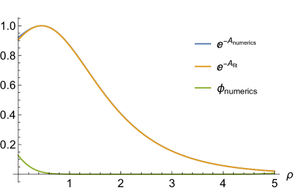
Figure 1: The profiles for $\phi$ (green) and $e^{-A}$ (blue) in our numerical solution compared to a fit (orange) of $e^{-A}$ to $\frac{1}{\cosh(\rho-\rho_{0})}$ where with the fit $\rho_{0}\approx 0.453$. Because this fit is very good our solution is well-approximated by a simple model of AdS₅ spacetime ending on a tensionful brane of tension $T\approx 1.27$.

For $\rho\lesssim 5$, however, we find that our solution is very well-approximated by pure AdS₅ cut off by a tensionful brane with tension $T\approx 1.27$, as plotted in Fig. 1. The deviations from pure AdS₅ are concentrated in the part of the spacetime very close to the ETW brane where $\phi$ is appreciable, and even then the deviations in $e^{-A}$ are only at the percent level.

An important property of holographic ETW branes is whether they are connected to the AdS part of the boundary by null geodesics that traverse a finite amount of boundary time. When that is the case two-point functions in the dual BCFT have singularities at cross-ratios other than those mandated by operator-product-expansion limits Reeves et al. (2021). As we show in Harvey et al. and discuss in the Appendix these null geodesics exist when

$$\phi_{b}=\int_{\bar{\rho}}^{\infty}d\rho\,e^{-A(\rho)}\,,$$ (23)

is less than $\pi$. As we explain in Harvey et al. we expect $\phi_{b}\geq\pi$ in healthy, UV-completable models of quantum gravity, in which case these singularities only appear when the dual BCFT is formulated on a hemisphere. Numerically evaluating this quantity we find $\phi_{b}\approx 2.01<\pi$.

We thus expect that our smeared ETW brane is somehow unstable. With that in mind consider the effective action for a single $\overline{\text{D}3}$ brane in the distribution,

$$S=-\frac{1}{(2\pi)^{3}\ell_{s}^{4}}\left(\int d^{4}\sigma\sqrt{-\text{P}[g]}-\int C_{4}\right)\,,$$ (24)

located at some point on the $\mathbb{S}^{5}$. When it sits at $\rho=\bar{\rho}$ it is extended along an AdS₄ submanifold inside of the five-dimensional part of the geometry, and its intersection with the conformal boundary of the space corresponds to the boundary of the dual BCFT.

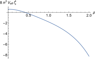
Figure 2: The effective potential for a single 3-brane as a function of its radial position $\rho$. The potential is globally maximized at $\rho=\bar{\rho}=0$, indicating an instability to separating from the smeared ETW brane.

Now suppose the brane sits at some other constant value of $\rho$, in which case it still ends on the boundary of the dual BCFT. The effective potential for $\rho$ is

$$V_{\rm eff}\propto e^{4A-\frac{20}{3}\phi}-4\int_{\bar{\rho}}^{\rho}d\rho^{\prime}e^{4A(\rho^{\prime})-\frac{40}{3}\phi(\rho^{\prime})}\,,$$ (25)

where the first term comes from the tension part of the brane action and the second from the Wess-Zumino term. We plot this effective potential in Fig. 2. It is extremized at $\rho=\bar{\rho}$, which it must since the angular part of the Israel junction condition implies force balance on the smeared ETW brane. However, the potential is not minimized at $\rho=\bar{\rho}$, but instead globally maximized. In fact the most energetically favorable possibility is that this single 3-brane separates from the rest of its distribution and tends towards the conformal boundary as $\rho\to\infty$. This is our anticipated instability.

Discussion. In this Letter we endeavoured to embed the simple model of Takayanagi (2011) for ETW branes in holography into the lamppost examples of AdS/CFT. We mandated that our supergravity backgrounds were invariant under rotations of the “internal space,” the $\mathbb{S}^{5}$ for the AdS${}_{5}\times\mathbb{S}^{5}$ vacuum of type IIB SUGRA, with an ETW brane dual to a conformal boundary of the dual CFT. Because these vacua are supported by RR fluxes the ETW brane carries RR charge, and in particular is a smeared distribution of branes. In the body of this Letter we presented a solution whereby an asymptotically AdS${}_{5}\times\mathbb{S}^{5}$ solution of type IIB SUGRA ends on a smeared distribution of 3-branes in such a way as to respect the appropriate analogue of the Israel junction condition. The ensuing geometry is quite nearly AdS${}_{5}\times\mathbb{S}^{5}$ for most of the spacetime up to a region very close to the smeared ETW brane. However, we found an instability whereby the individual 3-branes making up the ETW brane are unstable to the fluctuations of their transverse scalars.

While this solution is very well approximated by AdS${}_{5}\times\mathbb{S}^{5}$ cut off by a tensionful brane wrapping the $\mathbb{S}^{5}$, we stress that all of the details of type IIB SUGRA, including the effective potential for the $\mathbb{S}^{5}$ warpfactor and the angular part of the Israel junction condition, are all important in finding it. In particular, the angular part of the junction condition expresses the statement that the 3-branes at the end of the spacetime are in equilibrium, with the gravitational and RR forces on them balancing.

We also adapted our methods to search for $SO(6)$-invariant domain walls that connect two asymptotically AdS${}_{5}\times\mathbb{S}^{5}$ regions, one supported by $N_{+}$ units of five-form flux and the other by $N_{-}$ units. The putative domain wall is a smeared distribution of 3-branes that sources the difference in flux. It is straightforward to find the Israel junction condition for these putative interfaces as a function of the fluxes and to solve the equations of motion of type IIB SUGRA subject to those boundary conditions. However, unlike the ETW brane we found in the main text, we have not found solutions that respect the boundary conditions far away from the interface. We can tune initial conditions at an interface to achieve an asymptotically AdS${}_{5}\times\mathbb{S}^{5}$ region on one side of the interface, or the other, but not both.

Let us present a candidate for the (evidently, unstable) boundary condition dual to this unstable ETW brane. Since the ETW brane carries $N$ units of 3-brane charge, we have $N$ “color” branes ending on $N$ “ETW” branes. Let us for the moment take $N=1$. Our bulk solution suggests that this configuration would involve a single color brane and a single ETW brane in 10d flat space. In this suggestion there is a color brane extended in the $0123$ directions of flat space, ending on an ETW brane extended along the $0124$ directions at $x^{3}=0$. Both the color and ETW branes are semi-infinite, the former extended along $x^{3}>0$ and the latter along $x^{4}>0$. At small string coupling the semi-infinite color and ETW branes join into a single 3-brane. This is a non-supersymmetric, unstable “2 ND” intersection for which the boundary conditions for the fields on the color brane are known. In particular the scalar $\phi^{4}$ obeys a Neumann condition at $x^{3}=0$ but the remaining five scalars $\phi^{5,..,9}$ obey a Dirichlet condition. This configuration thus breaks the $SO(6)$ R-symmetry down to the $SO(5)$ that rotates the 56789 directions. For $N>1$ we can now consider $N$ semi-infinite color branes ending on $N$ semi-infinite ETW branes, with a similar $SO(6)\to SO(5)$ breaking boundary condition for each of the color branes, but now we can choose different $SO(5)$ subgroups for each. Such an arrangement will at finite $N$ completely break the $SO(6)$ R-symmetry. Our candidate dual to our bulk solution is precisely this in the $N\to\infty$ limit where the $SO(6)$ symmetry is restored by a uniform distribution of $SO(6)\to SO(5)$ breaking boundary conditions for each of the color branes.

From this point of view the instability of our ETW brane is perhaps not so surprising. However we stress that one necessarily confronts these 2 ND intersections when taking the model of Takayanagi (2011) seriously and attempting to embed it into string theory without using orientifolds.

There are two main lessons we learn from our analysis. The first is the importance of embedding models of ETW branes into string theory, especially from the point of view of checking stability. The second is that our solutions are non-trivial checks of the swampland criterion for ETW branes to appear in Harvey et al. , building on the work of Reeves et al. (2021), discussed in the last Subsection.

Acknowledgments. We would like to thank A. Karch, D. Neuenfeld, M. Rozali, J. Sorce, and J. Sully for enlightening discussions. This work was supported in part by an NSERC Discovery Grant.

Appendix A Light crossing and ETW branes

Consider the holographic dual of a BCFT, where the bulk spacetime has a line element

$$ds^{2}=d\rho^{2}+e^{2A(\rho)}\left(\frac{-dt^{2}+d\vec{x}^{2}+dz^{2}}{z^{2}}\right)\,,$$ (26)

for $\rho\geq\bar{\rho}$ with an ETW brane located at $\rho=\bar{\rho}$. In particular, consider the gravity dual of a two-point function of BCFT operators $\langle O(t_{1},\vec{x}_{1},z_{1})O(t_{2},\vec{x}_{2},z_{2})\rangle$. Owing to the existence of the boundary, conformal symmetry constrains this correlation function to be a kinematical prefactor times a function of a single conformally-invariant cross-ratio formed from $x_{1}$ and $x_{2}$. The authors of Reeves et al. (2021) have argued that these two-point functions have “unphysical” singularities, meaning singularities at cross-ratios that do not correspond to OPE limits either of the two $O$’s with each other, or an $O$ with the boundary, corresponding in the bulk to null geodesics that connect $x_{1}$ and $x_{2}$ by bouncing off the ETW brane. They show that this is the case both in the simple model Takayanagi (2011) of spacetime ending on a tensionful brane as well as for a stringy realization of an interface CFT, namely $\mathcal{N}=4$ super-Yang Mills subject to a supersymmetric Janus deformation. More generally one expects this to be true by the standard geometric optics argument for large dimension boundary operators, or by rewriting the boundary-to-boundary propagator as a sum over worldlines. The ensuing “unphysical” singularity is the AdS/BCFT version of the “looking for a bulk point” singularity of Maldacena et al. (2017).

However these null geodesics do not necessarily exist. Performing a coordinate transformation $d\phi=-e^{-A}d\rho$, the line element (26) becomes

$$ds^{2}=\frac{e^{2A(\rho)}}{z^{2}}\left(-dt^{2}+d\vec{x}^{2}+dz^{2}+z^{2}d\phi^{2}\right)\,.$$ (27)

From the coordinate transformation, we have

$$\phi=\int_{\rho}^{\infty}e^{-A(\rho^{\prime})}d\rho^{\prime}\,.$$ (28)

In this coordinate system, $\rho=\infty$ corresponds to $\phi=0$ and we define $\phi_{b}$ to be the location of ETW brane at $\rho=\bar{\rho}$. We note that $-dt^{2}+d\vec{x}^{2}+dz^{2}+z^{2}d\phi^{2}$ is just a wedge of flat space written as $\mathbb{R}^{d-1}$ times a wedge of $\mathbb{R}^{2}$ described in polar coordinates with $z$ the radius and $\phi$ the angle. Null geodesics in this space are just straight lines. One can always boost so that such a geodesic sits at constant $\vec{x}$, so that the motion takes place in $(t,z,\phi)$. Clearly, a null ray starting from AdS boundary cannot travel to the ETW brane if $\phi_{b}\geq\pi$. Therefore, the ETW brane can be reached from the AdS boundary by a null geodesic only when

$$\phi_{b}=\int_{\bar{\rho}}^{\infty}e^{-A}d\rho<\pi\,.$$ (29)

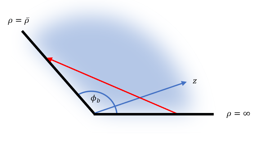
Figure 3: Null ray (red) traveling from the AdS boundary ($\rho=\infty$) to an ETW brane ($\rho=\bar{\rho}$) for $\phi_{b}<\pi$

Appendix B Smeared ETW branes in 11d SUGRA

In this Appendix we uncover realizations of smeared ETW branes in 11d SUGRA, in the context of the AdS${}_{4}\times\mathbb{S}^{7}$ and AdS${}_{7}\times\mathbb{S}^{4}$ vacua of M-theory. The derivation of these backgrounds closely follows that presented in the main text for the $SO(6)$-invariant compactification of type IIB SUGRA.

We begin with a brief primer to 11d supergravity, whose bosonic fields are a metric $G_{\mu\nu}$ and a Ramond-Ramond potential $C_{3}$. The bosonic action is given by

$$\begin{split}S_{11}=&\frac{1}{2\kappa^{2}_{11}}\int d^{11}x\sqrt{-G}\left(R-\frac{1}{2}|F_{4}|^{2}\right)\\ &\qquad\qquad-\frac{1}{12\kappa_{11}^{2}}\int C_{3}\wedge F_{4}\wedge F_{4}\,,\end{split}$$ (30)

and the field equations are

$$\begin{split}R_{MN}-\frac{R}{2}G_{MN}&=\frac{1}{2}F_{MPQR}F_{N}^{PQR}-\frac{1}{96}G_{MN}F_{PQRS}F^{PQRS}\,,\\ D_{M}F^{MNPQ}&=\frac{1}{2\times 4!^{2}}\epsilon^{NPQS_{1}...S_{4}T_{1}...T_{4}}F_{S_{1}...S_{4}}F_{T_{1}...T_{4}}\,,\end{split}$$ (31)

where $\epsilon^{NPQS_{1}...S_{4,7}T_{1}...T_{4,7}}$ is the 11d Levi-Civita tensor. These equations have AdS${}_{4}\times\mathbb{S}^{7}$ and AdS${}_{7}\times\mathbb{S}^{4}$ solutions respectively supported by a stack of M2 or M5 branes.

B.1 Asymptotically AdS${}_{4}\times\mathbb{S}^{7}$ geometries

We begin with the $SO(8)$ invariant compactification of 11d SUGRA on an $\mathbb{S}^{7}$, with $N$ units of flux through it. We parameterize the most general $SO(8)$-invariant line element and conserved four-form flux as

$$\begin{split}ds_{11}^{2}&=e^{-7\phi}g_{\mu\nu}dx^{\mu}dx^{\nu}+e^{2\phi}d\Omega^{2}_{4}\,,\\ F_{\mu\nu\rho\sigma}&=6L^{6}e^{-21\phi}\varepsilon_{\mu\nu\rho\sigma}\,,\end{split}$$ (32)

where $g_{\mu\nu}$ is a four-dimensional metric and $\epsilon_{\mu\nu\rho\sigma}$ its corresponding Levi-Civita tensor. This ansatz automatically satisfies the RR three-form equations of motion. The four-dimensional part of the 11d line element is scaled by the warpfactor $\phi(\rho)$ as a good choice of Weyl shift such that, upon dimensional reduction, the action is in Einstein-Hilbert form. Indeed, after dimensional reduction on the $\mathbb{S}^{7}$ the action reads

$$S_{4}=\frac{\text{vol}(\mathbb{S}^{7})}{2\kappa^{2}_{11}}\int d^{4}x\sqrt{-g}\left(R-\frac{63}{2}(\partial\phi)^{2}-V(\phi)\right)+(\text{bdy})\,,$$ (33)

where $R$ is the 4d scalar curvature and the potential is given by

$$V(\phi)=6e^{-9\phi}\left(3L^{12}e^{-12\phi}-7\right)\,,$$ (34)

with a unique minimum at $e^{\phi}=L$. Freezing $\phi$ to that value gives the Einstein-Hilbert action with negative cosmological constant

$$S_{4}=\frac{\text{vol}(\mathbb{S}^{7})}{2\kappa^{2}_{11}}\int d^{4}x\sqrt{-g}\left(R+\frac{24}{L^{9}}\right)+(\text{bdy})\,,$$ (35)

for $\Lambda=-\frac{12}{L^{9}}=-\frac{3}{L^{2}_{\rm eff}}$. We henceforth choose $L=1$ as a choice of units so that the effective AdS₄ radius is $L_{\rm eff}=\frac{1}{2}$. Small fluctuations of $\phi$ around this minimum, $\phi=\delta\phi$, are described by the quadratic action

$$S_{\rm quad}=-\frac{63\,\text{vol}(\mathbb{S}^{7})}{2\kappa^{2}_{11}}\int d^{4}x\sqrt{-g}\left(\frac{1}{2}(\partial\delta\phi)^{2}+\frac{9}{L^{2}_{\rm eff}}\delta\phi^{2}\right)\,.$$ (36)

These fluctuations have an effective mass-squared $m^{2}L^{2}_{\rm eff}=18$ so that the dual operator is dimension $\Delta=6$ and so irrelevant. Asymptotically AdS${}_{4}\times\mathbb{S}^{7}$ regions thus have $\phi\to 0$. For reference the equations of motion for $g_{\mu\nu}$ and $\phi$ are

$$R_{\mu\nu}-\frac{R}{2}g_{\mu\nu} =\frac{63}{2}\left(\partial_{\mu}\phi\partial_{\nu}\phi-\frac{1}{2}(\partial\phi)^{2}g_{\mu\nu}\right)$$ (37)

$$\qquad\quad-\frac{1}{2}6e^{-9\phi}\left(3L^{12}e^{-12\phi}-7\right)g_{\mu\nu}\,,$$

$$\square\phi =6e^{-9\phi}\left(1-L^{12}e^{-12\phi}\right)\,.$$

B.1.1 ETW brane

Mirroring the discussion in the main text we endeavor to put an $SO(8)$-invariant ETW brane into this geometry. Mandating that the bulk geometry has a $SO(2,2)\times SO(8)$ isometry we parameterize the 4d line element as

$$ds^{2}=e^{2A(\rho)}\left(\frac{-dt^{2}+dx^{2}+dz^{2}}{z^{2}}\right)+d\rho^{2}\,,$$ (38)

the warpfactor $\phi$ is fixed to be a function of $\rho$ alone, $\phi=\phi(\rho)$, and take the spacetime to exist only for $\rho\geq\bar{\rho}$ where the ETW brane is located. With this parameterization we have

$$F_{txz\rho}=\frac{6e^{-21\phi+3A}}{z^{3}}\Theta(\rho-\bar{\rho})\,.$$ (39)

This flux is conserved except at the ETW brane,

$$\begin{split}D_{M}F^{Mtxz}=\frac{6\sqrt{\tilde{g}}}{\sqrt{-G}}\delta(\rho-\bar{\rho})=\mathcal{S}^{txz}_{3}\,,\end{split}$$ (40)

where $\tilde{g}$ is the metric on a unit $\mathbb{S}^{7}$ and $\mathcal{S}_{3}$ encodes the RR charge density of the ETW brane. We infer that the boundary is equipped with a density of M2 branes uniformly distributed over the $\mathbb{S}^{7}$. The total boundary term is then a sum of the Gibbons-Hawking term together with the action of the distribution of M2 branes,

$$S_{\rm bdy} =\frac{1}{2\kappa_{11}^{2}}\bigg{(}2\int d^{10}x\sqrt{-H}\,K(H)$$ (41)

$$-6\left(\int d^{3}\sigma\,\sqrt{-\text{P}[G]}\wedge\Sigma+\int C_{3}\wedge\Sigma\right)\bigg{)}\,,$$

where $\Sigma=\text{vol}_{\mathbb{S}^{7}}=d^{7}\theta\sqrt{\tilde{g}}$ is the smearing form and $H$ is the induced metric on the boundary.

The analogue of the Israel Junction condition is

$$\begin{split}K(H)_{\mu\nu}-K(H)H_{\mu\nu}&=-3e^{-7\phi}H_{\mu\nu}\,,\\ K(H)_{\alpha\beta}-K(H)H_{\alpha\beta}&=0\,.\end{split}$$ (42)

Upon using the trace of the first line, the angular part can be shown to be equivalent to the statement that the distribution of M2 branes are in equilibrium. Expressed in terms of $A$ and $\phi$ the junction condition simplifies to

$$\begin{split}A^{\prime}&=-\frac{3}{2}e^{-\frac{21}{2}\phi}\,,\\ \phi^{\prime}&=-e^{-\frac{21}{2}\phi}\,.\end{split}$$ (43)

at $\rho=\bar{\rho}$.

B.1.2 Solution

We find it convenient to numerically solve the scalar equation along with the component of the Einstein’s equations in (53) obtained after contraction with the null vector $u^{\mu}\partial_{\mu}=ze^{-A}\partial_{t}+\partial_{\rho}$. These are

$$\begin{split}A^{\prime\prime}-e^{-2A}&=-\frac{63}{4}\phi^{\prime 2}\,,\\ \phi^{\prime\prime}+3A^{\prime}\phi^{\prime}&=6e^{-9\phi}\left(1-e^{-12\phi}\right)\,.\end{split}$$ (44)

Using the Israel junction condition (43), the $\rho\rho$-component of the Einstein’s equations imposes a further constraint on the data at $\rho=\bar{\rho}$,

$$e^{-2A}=7e^{-9\phi}\,.$$ (45)

This, together with the junction condition, determines $(A,\phi^{\prime},A^{\prime})$ in terms of $\phi$ there.

Our strategy is to solve the equations (44) by shooting from $\rho=\bar{\rho}$ and dialing the “initial condition” $\phi(\bar{\rho})$ until we achieve the asymptotically AdS${}_{4}\times\mathbb{S}^{7}$ boundary condition $\phi\to 0$ as $\rho\to\infty$. We are unable to impose this boundary condition exactly, but we have found a solution which obeys it up to a fairly large value of $\rho\lesssim 4$. The solution is plotted in Fig. 4. The 4d part of the solution is very close to pure AdS₄ cut off by a tensionful brane of tension $T\approx 1.89$.

We have discussed the quantity $\phi_{b}$, which when $<\pi$ indicates that the ETW brane can be reached by a null geodesic from the AdS boundary. This solution has

$$\phi_{b}=\int_{0}^{\infty}d\rho\,e^{-A(\rho)}\approx 2.06<\pi\,.$$ (46)

We also consider the effective potential for a single M2 brane separated from the distribution at $\rho=\bar{\rho}=0$, but extended along an AdS₃ slice at constant $\rho$ and at a fixed angle on the $\mathbb{S}^{7}$. Its effective potential obeys

$$V_{\rm eff}\propto e^{3A-\frac{21}{2}\phi}-6\int^{\rho}_{0}d\rho^{\prime}\,e^{3A(\rho^{\prime})-21\phi(\rho^{\prime})}\,,$$ (47)

and it is globally maximized at $\rho=0$. As for our smeared distribution of 3-branes, this indicates an instability to fragmentation.

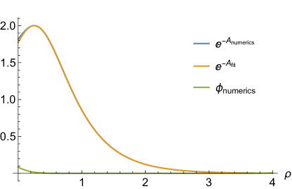
Figure 4: The numerical profiles for $\phi(\rho)$ (green) and $e^{-A(\rho)}$ (blue) for an asymptotically AdS${}_{4}\times\mathbb{S}^{7}$ geometry ending on a distribution of M2 branes at $\rho=0$. The 4d geometry is very close to that of empty AdS₄ ending on a tensionful brane of tension $T\approx 1.89$, as indicated by the fit (orange).

B.2 Asymptotically AdS${}_{7}\times\mathbb{S}^{4}$ geometries

Now consider the $SO(5)$-invariant compactification on a $\mathbb{S}^{4}$ with $N$ units of flux through it. The most general line element and conserved four-form flux consistent with $SO(5)$ isometry are

$$\begin{split}ds^{2}&=e^{-\frac{8}{5}\phi}g_{\mu\nu}dx^{\mu}dx^{\nu}+e^{2\phi}d\Omega^{2}_{4}\,,\\ F_{\alpha\beta\gamma\delta}&=3L^{3}\varepsilon_{\alpha\beta\gamma\delta}\,,\end{split}$$ (48)

where $\varepsilon_{\alpha\beta\gamma\delta}$ is the Levi-Civita tensor on a unit $\mathbb{S}^{4}$. The flux satisfies the RR equations of motion. The seven-dimensional effective action is

$$S_{7}=\frac{\text{vol}(\mathbb{S}^{4})}{2\kappa^{2}_{11}}\int d^{7}x\sqrt{-g}\left(R-\frac{36}{5}(\partial\phi)^{2}-V(\phi)\right)+(\text{bdy})\,,$$ (49)

where $R$ is the 7d scalar curvature and the potential is

$$V(\phi)=3e^{-\frac{18}{5}\phi}\left(\frac{3L^{6}}{2}e^{-6\phi}-4\right)\,,$$ (50)

which has a unique minimum at $e^{\phi}=L$. Freezing $\phi$ to that value gives the Einstein-Hilbert action with negative cosmological constant

$$S_{7}=\frac{\text{vol}(\mathbb{S}^{4})}{2\kappa^{2}_{11}}\int d^{7}x\sqrt{-g}\left(R+\frac{15}{2L^{\frac{18}{5}}}\right)+(\text{bdy})\,,$$ (51)

i.e. $\Lambda=-\frac{15}{4L^{\frac{18}{5}}}=-\frac{15}{L^{2}_{\rm eff}}$. We henceforth work in $L=1$ units for which $L_{\rm eff}=2$. Small fluctuations of $\phi$ around the minimum are described by a quadratic action

$$S_{\rm quad}=-\frac{72\,\text{vol}(\mathbb{S}^{4})}{10\kappa^{2}_{11}}\int d^{7}x\sqrt{-g}\left(\frac{1}{2}(\partial\delta\phi)^{2}+\frac{36}{L^{2}_{\rm eff}}\delta\phi^{2}\right)\,.$$ (52)

These fluctuations have an effective mass-squared $m^{2}L^{2}_{\rm eff}=72$, and so the dual operator is irrelevant with $\Delta=12$. Asymptotically AdS${}_{7}\times\mathbb{S}^{4}$ geometries then have $\phi\to 0$. For reference the equations of motion are

$$R_{\mu\nu}-\frac{R}{2}g_{\mu\nu} =\frac{36}{5}\left(\partial_{\mu}\phi\partial_{\nu}\phi-\frac{1}{2}(\partial\phi)^{2}g_{\mu\nu}\right)$$ (53)

$$\qquad-\frac{3}{2}e^{-\frac{18}{5}\phi}\left(\frac{3L^{6}}{2}e^{-6\phi}-4\right)g_{\mu\nu}\,,$$

$$\square\phi =3e^{-\frac{18}{5}\phi}\left(1-L^{6}e^{-6\phi}\right)\,.$$

B.2.1 ETW brane

We would like to find an asymptotically AdS${}_{7}\times\mathbb{S}^{4}$ geometry that ends on an ETW brane in an $SO(5)$-invariant way, and for which the ETW brane is dual to a conformally invariant boundary condition. Such a geometry is invariant under an $SO(2,5)\times SO(5)$ isometry and is constrained to take the form

$$ds^{2}_{7}=e^{2A(\rho)}\left(\frac{-dt^{2}+d\vec{x}^{2}+dz^{2}}{z^{2}}\right)+d\rho^{2}\,,$$ (54)

together with $\phi=\phi(\rho)$. The seven-form flux then reads

$$F_{t1\ldots 4z\rho}=\frac{3e^{-\frac{48}{5}\phi+6A}}{z^{6}}\Theta(\rho-\bar{\rho})\,,$$ (55)

which is conserved except at the ETW brane. Its divergence computes the RR charge density of the ETW brane,

$$\begin{split}D_{M}F^{Mt1234z}=-\frac{3\sqrt{\tilde{g}}}{\sqrt{-G}}\delta(\rho-\bar{\rho})=\mathcal{S}^{t1\ldots 4z}_{6}\,,\end{split}$$ (56)

corresponding to a uniform distribution of $\overline{\text{M}5}$ branes smeared over the $\mathbb{S}^{4}$. The boundary term in the action is then the sum of the Gibbons-Hawking term and the action for this distribution of $\overline{\text{M}5}$ branes,

$$S_{\rm bdy} =\frac{1}{2\kappa_{11}^{2}}\bigg{(}2\int d^{10}x\sqrt{-H}\,K(H)$$ (57)

$$\quad-3\left(\int d^{6}\sigma\,\sqrt{-\text{P}[G]}\wedge\Sigma+\int C_{6}\wedge\Sigma\right)\bigg{)}\,,$$

where $\Sigma=\text{vol}_{\mathbb{S}^{4}}=d^{4}\theta\sqrt{\tilde{g}}$ is the smearing form with $\tilde{g}$ the metric on a unit $\mathbb{S}^{4}$.

The corresponding Israel junction conditions at $\rho=\bar{\rho}$ read

$$\begin{split}K(H)_{\mu\nu}-K(H)H_{\mu\nu}&=-\frac{3}{2}e^{-4\phi}H_{\mu\nu}\,,\\ K(H)_{\alpha\beta}-K(H)H_{\alpha\beta}&=0\,.\end{split}$$ (58)

Using the trace of the first line, the angular part implies that the $\overline{\text{M}5}$ branes are in equilibrium. In terms of the quantities $A$ and $\rho$ the junction conditions become

$$\begin{split}A^{\prime}&=-\frac{3}{10}e^{-\frac{24}{5}\phi}\,,\\ \phi^{\prime}&=-e^{-\frac{24}{5}\phi}\,,\end{split}$$ (59)

at $\rho=\bar{\rho}$.

B.2.2 Solution

We seek to find an asymptotically AdS${}_{7}\times\mathbb{S}^{4}$ solution consistent with the ETW boundary condition (59). Again it is convenient to solve the $uu$ component of the Einstein’s equations in (53), where $u^{\mu}\partial_{\mu}=ze^{-A}\partial_{t}+\partial_{\rho}$, along with the scalar equation of motion. These are

$$\begin{split}A^{\prime\prime}-e^{-2A}&=-\frac{36}{25}\phi^{\prime 2}\,,\\ \phi^{\prime\prime}+6A^{\prime}\phi^{\prime}&=3e^{-\frac{18}{5}\phi}\left(1-e^{-6\phi}\right)\,.\end{split}$$ (60)

Using the junction condition (59) the $\rho\rho$-component of Einstein’s equations imposes a further constraint on the data at $\rho=\bar{\rho}$,

$$e^{-2A}=\frac{2}{5}e^{-\frac{18}{5}\phi}\,.$$ (61)

The data $(A,\phi^{\prime},A^{\prime})$ at $\rho=\bar{\rho}$ are then determined in terms of $\phi$ there which acts as an initial condition for our numerical evolution.

We then shoot from the ETW brane subject to these boundary conditions and tune the initial condition $\phi(\bar{\rho})$ so as to achieve the asymptotically AdS${}_{7}\times\mathbb{S}^{4}$ boundary condition $\phi\to 0$ as $\rho\to\infty$. We have found a solution, presented in Fig. 5, which accomplishes this for fairly large $\rho\lesssim 7$. For that solution we have also computed

$$\phi_{b}=\int_{0}^{\infty}d\rho\,e^{-A(\rho)}\approx 2.26<\pi\,,$$ (62)

which implies that the ETW brane and the AdS₇ boundary are connected by null geodesics. As with our other examples the noncompact part of the geometry is quite nearly pure AdS, cut off by a tensionful brane of tension $T\approx 0.974$.

We have also studied the effective potential for a single $\overline{\text{M}5}$ brane separated from the rest of the distribution. As in our examples above its effective potential for $\rho$, provided that it is extended along an AdS₆ slice and sitting at a fixed angle on the $\mathbb{S}^{4}$, is globally maximized at $\rho=\bar{\rho}=0$. As a result this ETW brane is also unstable to fragmentation.

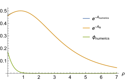
Figure 5: The numerical profiles for $\phi(\rho)$ (green) and $e^{-A(\rho)}$ (blue) for our asymptotically AdS${}_{7}\times\mathbb{S}^{4}$ geometry that ends on a distribution of $\overline{\text{M}5}$ branes at $\rho=0$. The 7d geometry is quite nearly empty AdS₇ cut off by a tensionful brane of tension $T\approx 0.974$ as indicated by the fit (orange).