Primordial Black Holes from Conformal Higgs

Abstract

Scale-invariant extensions of the electroweak theory are not only attractive because they can dynamically generate the weak scale, but also due to their role in facilitating supercooled first-order phase transitions. We study the minimal scale-invariant $U(1)_{\rm D}$ extension of the standard model and show that Primordial Black Holes (PBHs) can be abundantly produced. The mass of these PBHs is bounded from above by that of the moon due to QCD catalysis limiting the amount of supercooling. Lunar-mass PBHs, which are produced for dark Higgs vev $v_{\phi}\simeq 20\leavevmode\nobreak\ \rm TeV$, correspond to the best likelihood to explain the HSC lensing anomaly. For $v_{\phi}\gtrsim 400\leavevmode\nobreak\ \rm TeV$, the model can explain hundred per cent of dark matter. At even larger hierarchy of scales, it can contribute to the $511\leavevmode\nobreak\ \rm keV$ line. While the gravitational wave (GW) signal produced by the HSC anomaly interpretation is large and detectable by LISA above astrophysical foreground, the dark matter interpretation in terms of PBHs can not be entirely probed by future GW detection. This is due to the dilution of the signal by the entropy injected during the decay of the long-lived $U(1)_{\rm D}$ scalar. This extended lifetime is a natural consequence of the large hierarchy of scales.

I.   INTRODUCTION

Stellar-mass and supermassive black holes are at the forefront of astrophysical research, particularly following the detection of gravitational waves by LIGO/Virgo [1] and Pulsar Timing Arrays (PTA) [2, 3, 4]. However, general relativity allows black holes to have any mass. Sub-solar mass black holes can form from the gravitational collapse of large overdensities in the primordial plasma [5] and could explain $100\leavevmode\nobreak\ \%$ of the observed dark matter relic density in the mass range $10^{-16}M_{\odot}\lesssim M_{\rm PBH}\lesssim 10^{-10}M_{\odot}$ [6, 7, 8, 9]. The production of Primordial Black Holes (PBHs) by “late-blooming” during supercooled first-order phase transition, introduced in 1981 [10, 11, 12, 13, 14, 15], has received considerable attention recently [16, 17, 18, 19, 20, 21, 22, 23, 24, 25], also in relation with the PTA signal [26, 27, 28, 29].

In this letter, we investigate whether the electroweak phase transition (EWPT), minimally extended by new physics, can generate PBHs. Apart from its second derivative around $\left<H\right>\simeq 246\leavevmode\nobreak\$GeV measured in 2011 [30, 31], the shape of the Higgs potential remains unconstrained [32]. In 1976, Gildener and S. Weinberg [33] suggested that the Higgs mass could vanish at tree level and be dynamically generated when quantum loop corrections, introduced by Coleman and E. Weinberg (CW) in 1973 [34], drive the Higgs quartic to negative values in the infrared. The original model has been ruled out by the large top mass [35], necessitating the introduction of additional bosonic fields into the Standard Model (SM) to make it viable. One of the simplest scale-invariant extensions of electroweak theory involves a complex scalar field $\phi$, neutral under the SM but charged under an additional $U(1)_{\rm D}$ gauge group [35]. This model has attracted considerable attention due to its small number of new parameters and potential implications for dark matter, leptogenesis and neutrino oscillations [36, 37, 38, 39, 40, 41, 42, 43, 44, 45]. Phase transitions driven by a Coleman-Weinberg potential plus thermal corrections:

$$V(\phi)\simeq\frac{g^{2}T^{2}\phi^{2}}{2}+\frac{\beta_{\lambda}\phi^{4}}{4}\left[\log{\left(\frac{\phi}{v_{\phi}}\right)-\frac{1}{4}}\right],$$ (1)

are known to be strongly first order (1stOPT) and supercooled [46, 47]. We have Taylor-expanded thermal corrections around the symmetric minima $\phi=0$. We have introduced the beta function $\beta_{\lambda}$ of the quartic coupling $\lambda\phi^{4}$ and the coupling $g$ with particles of the plasma. For the $U(1)_{\rm D}$ model with gauge coupling $g_{\rm D}$ studied in this letter, one has $\beta_{\lambda}\simeq 3g_{\rm D}^{4}/8\pi^{2}$ and $g^{2}\simeq g_{\rm D}^{2}/12$. Spontaneous breaking $\left<\phi\right>\neq 0$ is communicated to the Higgs field $H$ through the mixing $\lambda|H|^{2}\phi^{2}$. The scalar $\phi$ can be interpreted as the “Higgs of the Higgs” [48]. Thanks to the logarithmic potential, the temperature $T_{n}$ at which bubbles nucleate and percolate is exponentially suppressed for $\beta_{\lambda}\ll 1$:

$$T_{n}\leavevmode\nobreak\ \ll\leavevmode\nobreak\ T_{c}\,\exp\left(-\frac{16\pi}{3S_{\rm c}}\frac{g}{\beta_{\lambda}}\right),\quad S_{c}\simeq 130,$$ (2)

with respect to the critical temperature $T_{c}$ when the 1stOPT becomes energetically allowed. $S_{c}$ is the bounce action at percolation. Coleman-Weinberg dominance in the potential in Eq. (1) additionally implies that the bounce action cost $S_{3}/T$ – which controls the bubble nucleation rate per unit of volume $\Gamma_{{\rm V}}=T^{4}\exp(S_{3}/T)$ – decreases only logarithmically with the temperature. This implies that the completion rate of the PT:

$$\beta\leavevmode\nobreak\ \equiv\leavevmode\nobreak\ \frac{d\log{\Gamma_{{\rm V}}}}{dt}\simeq\left(\frac{3\beta_{\lambda}}{16\pi g}S_{c}^{2}-4\right)H,$$ (3)

can be relatively small for $\beta_{\lambda}\ll 1$.

We investigate the minimal $U(1)_{D}$ scale-invariant extension of the electroweak theory. We study the tunneling dynamics both numerically [49] and analytically taking into account QCD catalysis and collider constraints. We find that the two essential conditions for the formation of PBHs in observable quantities – significant supercooling ($T_{n}\ll T_{c}$) and a slow rate of completion ($\beta/H\lesssim 8$) [21] – can be satisfied as soon as the Dark Higgs Vacuum Expectation Value (VEV) is larger than $v_{\phi}\gtrsim 10\leavevmode\nobreak\ \rm TeV$. The mass of the PBH is given by the mass of the moon or smaller, giving possible explanation of lensing anomalies [50, 51, 52], Dark Matter [6, 7, 8, 9], the 511 keV excess [53, 54, 55] and other cosmic rays [56, 57, 58, 59, 60, 61, 62, 63, 64, 65, 66]. The gravitational wave detection prospects are calculated in all the parameter space, accounting for astrophysical foregrounds. We account for the matter era following the phase transition resulting from the dark Higgs becoming long-lived at large VEV.

II.   SCALE INVARIANT EXTENSION OF THE ELECTROWEAK THEORY

The scalar potential — We extend the SM with a complex scalar field $\Phi$ charged under a hidden $U(1)_{\rm D}$ dark photon $V_{\mu}$ with coupling constant $g_{\rm D}$ [35]:

$$\mathcal{L}_{\rm tree}=\left|D_{\mu}\Phi\right|^{2}-V_{\rm tree}(|\Phi|,|H|),$$ (4)

with $D_{\mu}=\partial_{\mu}+ig_{\rm D}t^{a}V_{\mu}^{a}$. Supposing Bardeen’s conjecture that scale-invariance is a fundamental symmetry of Nature at tree level [67], the only allowed operators in the scalar potential are:

$$V_{\rm tree}(|\Phi|,|H|)=\lambda_{h}|H|^{4}+\lambda_{\phi}|\Phi|^{4}-\lambda_{h\phi}|\Phi|^{2}|H|^{2},$$ (5)

where $\lambda_{h\phi}$ is the mixing coupling with the SM Higgs $H$. In the unitarity gauge, we can parameterize the scalar fields as:

$$H=\left(0,\frac{h}{\sqrt{2}}\right),\qquad\Phi=\frac{\phi}{\sqrt{2}}.$$ (6)

Scale-invariance is violated by quantum interactions encoded in Renormalized Group Equations (RGE), see e.g. [41]. In App. B, we show that upon assuming the ordering $g_{\rm D}^{2}\gg\lambda_{\phi},\lambda_{h\phi}$, the 1-loop corrected potential is well approximated by its leading-log term:

$$V_{T=0}(\phi)=\beta_{\lambda}\frac{\phi^{4}}{4}\left[\textrm{log}\left(\frac{\phi}{v_{\phi}}\right)-\frac{1}{4}\right],\quad\beta_{\lambda}\simeq 6\alpha_{\rm D}^{2}.$$ (7)

We use the full RGE improved coupling $\lambda_{\phi}(\phi)$ in our numerical computations. The Coleman-Weinberg potential in Eq. (7) generates a VEV for the $U(1)_{\rm D}$ field $\left<\phi\right>=v_{\phi}$, which through the mixing $\lambda_{h\phi}h^{2}\phi^{2}$ generates a VEV for the Higgs $\left<h\right>=v_{\rm EW}$. Fixing the Higgs VEV to $v_{\rm EW}=246\leavevmode\nobreak\ \rm GeV$ and its mass to $m_{h}=125\leavevmode\nobreak\ \rm GeV$ implies:

$$\lambda_{h}=\frac{m_{h}^{2}}{2v_{\rm EW}^{2}}\simeq 0.13,\quad\lambda_{h\phi}=\frac{m_{h}^{2}}{v_{\phi}^{2}}\simeq 0.02\left(\frac{1\leavevmode\nobreak\ \rm TeV}{v_{\phi}}\right)^{2}.$$ (8)

At finite temperature the potential for $\phi$ receives thermal corrections which under the ordering $g_{\rm D}^{2}\gg\lambda_{\phi},\lambda_{h\phi}$ are dominated by the dark photon $V_{\mu}$. The 1-loop and Daisy contributions read [68]:

$$V_{\rm T}(\phi)=\frac{T^{4}}{2\pi^{2}}J_{B}\left(\frac{m_{V}^{2}(\phi)}{T^{2}}\right)+\frac{T}{12\pi}\left[m_{V}^{3}-\left(m_{V}^{2}+\Pi_{V}\right)^{3/2}\right],$$ (9)

with $m_{V}^{2}(\phi)=g_{\rm D}^{2}\phi^{2}$ and $\Pi_{V}=g_{\rm D}^{2}T^{2}/6$ [69].
QCD catalysis — In App. B, we show that the motion of the Higgs field can be safely neglected during the tunneling if $v_{\phi}\gtrsim\leavevmode\nobreak\ \rm TeV$. An exception arises if the universe super-cools below the temperature of QCD confinement $T_{n}\lesssim\Lambda_{\rm QCD}$. Then the top chiral condensate induces a negative linear slope in the Higgs direction $-\frac{y_{t}}{\sqrt{2}}\left<t_{\rm L}t_{\rm R}\right>h$ [47], see also [70, 71, 72, 73, 74, 75, 76]. The Higgs acquires a VEV $\left<h\right>_{{\rm QCD}}^{3}=\frac{4y_{t}}{\sqrt{2}\lambda_{h}}\left<t_{\rm L}t_{\rm R}\right>\sim\Lambda_{\rm QCD}^{3}$ which through the mixing $\lambda_{h\phi}$ induces a negative mass for the hidden scalar $\phi$:

$$V_{\rm QCD}(\phi)=-\frac{1}{4}\lambda_{h\phi}\left<h\right>_{{\rm QCD}}^{2}\phi^{2}\Theta(T-\Lambda_{\rm QCD}).$$ (10)

Since both the Higgs quartic $\lambda_{h}$ and the top Yukawa $y_{t}$ diverges below $\Lambda_{\rm QCD}$, it is not possible to predict the precise value of $\left<h\right>_{{\rm QCD}}$ [72, 75]. Waiting for further studies, we approximate the temperature dependence of QCD effects with a $\Theta$ function and fix $\left<h\right>_{{\rm QCD}}=100\leavevmode\nobreak\ \rm MeV$.
Bubble nucleation — The thermal corrections in Eq. (9) generates a barrier between the minima in $\phi=0$ and $\phi=v_{\phi}$. Thermal fluctuation can drive the field over the barrier with a rate per unit of volume [77]:

$$\Gamma_{{\rm V}}(T)\simeq T^{4}\left(\frac{S_{3}/T}{2\pi}\right)^{3/2}{\rm exp}\left(-S_{3}/T\right),$$ (11)

where $S_{3}$ is the $O_{3}$-symmetric bounce action. We wrote a C++ undershooting-overshooting software program ${\tt CCBounce}$ [49] to find the tunneling trajectory and compute the bounce action $S_{3}$. We found it to be well approximated by the thick-wall formula:

$$\frac{S_{3}}{T}\simeq\frac{A}{\textrm{log}\left(\frac{M}{T}\right)}\quad\text{with}\quad M=0.43\,g_{\rm D}\,v_{\phi},\quad$$ (12)

$$A=\frac{127.3}{g_{\rm D}^{3}}\sqrt{1-\left(\frac{T_{{\rm QCD}}}{T}\right)^{\!2}},\quad T_{{\rm QCD}}=\frac{\sqrt{6\lambda_{\rm h\sigma}}}{g_{\rm D}}\left<h\right>_{{\rm QCD}}.$$

$T_{{\rm QCD}}$ is the temperature when the QCD contribution in Eq. (10) becomes larger than the thermal barrier of $\phi$ and below which the EW-PT must necessarily complete. We refer to App. B for more details on the bounce action calculation and in particular Fig. 5 for a comparison of the thick-wall formula with the proper numerical treatment.

Nucleation happens when the decay rate in Eq. (11) multiplied by the causal volume becomes comparable to the Hubble expansion rate: $\Gamma_{{\rm V}}(T_{n})\simeq H^{4}(T_{n})$. Plugging Eq. (12), we deduce the nucleation temperature:

$$T_{n}/T_{\rm eq}\simeq 5\,\exp\left[-\frac{127}{g_{\rm D}^{3}S_{c}}\right],\quad S_{c}\simeq 4\ln{\frac{T_{n}}{H(T_{n})}}\simeq 130,$$ (13)

where we neglected the QCD contribution for clarity. We use a proper root solving algorithm to find $T_{n}$ in our plots. In the absence of QCD, effects, the bounce action $S_{3}/T$ flattens at low temperature, causing the absence of solution for $\Gamma_{{\rm V}}(T_{n})\simeq H^{4}(T_{n})$ below the temperature [78, 79, 80]:

$$T_{n}^{\rm min}\simeq\sqrt{MH_{n}},$$ (14)

where $H_{n}\equiv H(T_{n})$ and $M$ given by Eq. (12). Instead, QCD confinement generates a sharp decrease of $S_{3}/T$ down to zero below the temperature $T_{{\rm QCD}}$.

We can now evaluate the rate of PT completion $\beta\equiv d\log{\Gamma_{{\rm V}}}/dt$ at nucleation. Above QCD confinement $T_{n}\gg T_{{\rm QCD}}$, it decreases logarithmically with the temperature

$$\beta/H_{n}\simeq-4+\frac{127}{g_{\rm D}^{3}\ln^{2}{\left(\frac{M}{T_{n}}\right)}}.$$ (15)

Instead, around $T_{n}\sim T_{{\rm QCD}}$ the PT completion rate diverges as $\beta/H_{n}\propto 1/(T_{{\rm QCD}}-T_{n})$. We conclude that the PT rate $\beta/H$ is minimized for coupling $g_{\rm D}$ associated with the longest supercooling stage while not being catalyzed by QCD $\Lambda_{\rm QCD}\lesssim T_{n}\ll T_{\rm eq}$. The nucleation temperature $T_{n}$ and the PT rate $\beta/H_{n}$ in scale-invariant SM+$U(1)_{\rm D}$ are shown in Fig. 1.

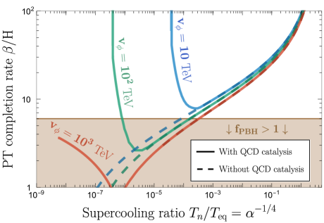
Figure 1: The PT completion rate $\beta/H$ becomes lower as the amount of supercooling increases, until QCD effects kick in around $T_{n}\simeq T_{{\rm QCD}}$ in Eq. (12). The lines are obtained from varying $g_{\rm D}$. The parameter $\alpha$ along the horizontal axis is the latent heat fraction.

The latent heat $\Delta V\simeq\beta_{\lambda}v_{\phi}^{4}/16$ dominates the energy density of the universe, generating an inflationary period, below the temperature $T_{\rm eq}$:

$$T_{\rm eq}\simeq\frac{g_{\rm D}v_{\phi}}{10.85}\left(\frac{100}{g_{*}}\right)^{1/4}.$$ (16)

Reheating after matter domination — Supercooled PTs proceed with ultra-relativistic bubble wall Lorentz factor $\gamma\gg 1$ [81, 82, 83, 84]. Bubble growth convert the latent heat into scalar field gradient stored in the walls and plasma excitation resulting from the friction operating on the walls. The fraction stored in the former at percolation is given by:

$$\kappa_{\rm coll}=\frac{\gamma_{\rm coll}}{\gamma_{\rm max}},$$ (17)

where $\gamma_{\rm coll}$ is the wall Lorentz factor at collision accounting for friction [83], while $\gamma_{\rm max}$ is the same quantity neglecting friction. We refer to App. C for the details. The main dark Higgs decay channel is into two Higgs $\phi\to hh$. However the decay rate is suppressed by the small mixing $\lambda_{h\phi}$:

$$\Gamma_{\phi\to hh}=\frac{\lambda_{h\phi}^{2}v_{\phi}^{2}}{32\pi m_{\phi}}=0.3H_{n}\left(\frac{0.5}{g_{\rm D}}\right)^{6}\left(\frac{10^{3}\leavevmode\nobreak\ \rm TeV}{v_{\phi}}\right)^{5},$$ (18)

where $m_{\phi}=\beta_{\lambda}v_{\phi}$ is the scalar mass and $H_{n}^{2}=\Delta V/3M_{\rm pl}^{2}$ is the Hubble rate at percolation. The other decay channel, through Higgs mixing, is further suppressed by $(v_{\rm EW}/v_{\phi})^{2}$:

$$\Gamma_{\phi\to h\to SM}=\Gamma_{h}\sin^{2}(\theta_{h\phi})\simeq\Gamma_{h}\left(\frac{3\lambda_{h\phi}v_{\rm EW}}{11\beta_{\lambda}v_{\phi}}\right)^{2},$$ (19)

where $\Gamma_{h}\simeq 4.1\leavevmode\nobreak\ \rm MeV$ is Higgs decay width [85] and $\theta_{h\phi}$ is the angle diagonalizing the mass matrix given by Eq. (74) in App. B. The universe after percolation contains a matter component occupying a fraction $\kappa_{\rm coll}$ in Eq. (17) of the total energy density. According to Eq. (18), this matter component is long-lived for $v_{\phi}\gtrsim 10^{3}\leavevmode\nobreak\ \rm TeV$. It dominates the universe below the temperature:

$$T_{\rm dom}=\kappa_{\rm coll}T_{\rm eq},$$ (20)

hence generating an early matter-domination (MD) era, which ends with the decay of $\phi$ at the temperature:

$$T_{\rm dec}=\frac{1.2}{g_{*}^{1/4}}\sqrt{M_{\rm pl}\Gamma_{\phi}}.$$ (21)

The decay of $\phi$ reheates the SM and dilutes the abundance of any relics decoupled from the SM with a factor:

$$D=1+\frac{T_{\rm dom}}{T_{\rm dec}}.$$ (22)

As discussed in the next section, this will have a minor impact on the PBH detectability but a major impact on the GW one.

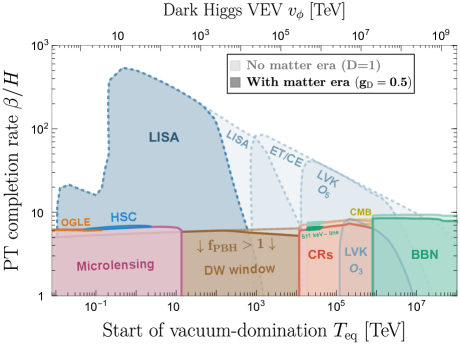
Figure 2: In an adiabatic universe, supercooled phase transition produce gravitational waves within the frequency window of future interferometers LVK run O3 [86], run $O_{5}$ [87], ET/CE [88, 89, 90] and LISA [91, 92, 93, 94] with an amplitude larger than astrophysical foregrounds from white dwarfs binaries and compact binaries [95, 96, 92, 97, 86]. Instead, in the minimal scale-invariant extension of the SM, the long lifetime of the scalar field dilute all the GW signals at large dark Higgs VEV $v_{\phi}\gtrsim 10^{4}\leavevmode\nobreak\ \rm TeV$. Instead the PBH abundance is only slighly impacted by the matter era. See Fig. 9 in App. C for more details on the experiments reach and expected astrophysical foregrounds.

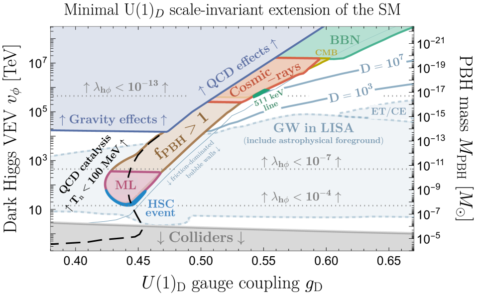
Figure 3: PBH and GW predictions in the minimal scale-invariant $U(1)_{\rm D}$ extension of the SM. The model has only two parameters: the hidden $U(1)_{\rm D}$ breaking scale $v_{\phi}$ and its gauge coupling $g_{\rm D}$. The purple region shows the microlensing constraints (ML) from HSC/subaru telecope [98, 99]. The blue U-shaped region can explain the HSC event [100, 51, 52]. The boundary of the brown region can explain dark matter. Hawking evaporation overproduce cosmic rays in the red region [53, 54, 55, 56, 57, 58, 59, 60, 61], but could contribute to the $511\leavevmode\nobreak\ \rm keV$ excess in the green spot [53, 54, 55]. Non-observation of energy injection from Hawking radiation in CMB [101, 102, 103] and BBN [56, 104, 105] exclude the yellow and green regions. See [8] for a review of PBH constraints. The GW constraints shown in light blue disappear at large $v_{\phi}\gtrsim 10^{4}\leavevmode\nobreak\ \rm TeV$ due to entropy injection following the decay of the long-lived dark Higgs. The associated dilution factor $D$ is indicated with blue lines labelled “D”. Part of the PBH DM region can not be probed with GWs. On the left of the dashed black line, the PT is catalysed by QCD confinement. In the blue region in the top-left corner, the universe can not tunnel without “QCD effects”, due to $\Gamma_{{\rm V}}=H^{4}$ having no solution $T_{n}$. However, the QCD catalysis temperature given in Eq. (12) is smaller than the Hubble scale $T_{{\rm QCD}}\lesssim H_{n}$, implying that the tunneling dynamics receives large correction from “gravity effects” [106, 107], which we leave for future research. The gray region displays collider constraints on additional Higgs boson [108, 109, 110, 111], see Fig. 8 for more details. On the right of the very thin blue line, bubble wall friction convert most of the the latent heat into the plasma, which reduces the energy fraction stored in the scalar field and therefore reduces the dilution factor $D$.

III.   PHENOMENOLOGY

Primordial black holes — Due to the stochastic nature of thermal tunneling, distinct causal patches percolate at slightly different times. Patches which percolate later hold the latent heat longer in the form of vacuum energy while their neighbors already released it into radiation-like energy density. When the latest patches finally percolate, they are overdense which, beyond a given threshold, lead to their collapse into PBHs. The PBH mass is given by the mass within the sound horizon at the time of percolation:

$$M_{\rm{PBH}}\simeq M_{\mathMoon}\leavevmode\nobreak\ \left(\frac{0.5}{g_{\rm D}}\right)^{2}\left(\frac{\lambda_{h\phi}}{1.2\times 10^{-4}}\right),$$ (23)

where $M_{\mathMoon}\simeq 3.7\times 10^{-8}M_{\odot}$ is the moon mass. The steps leading to the PBH abundance are reviewed in App. A following [21]. Normalised to the dark matter relic density, it gives:

$$f_{\rm{PBH}}\simeq\frac{1}{D}\left(\frac{\mathcal{P}_{\rm coll}}{3.1\times 10^{-12}}\right)\left(\frac{T_{\rm eq}}{1\leavevmode\nobreak\ \rm TeV}\right)\,.$$ (24)

where $\mathcal{P}_{\rm coll}$ is the fraction of causal patches collapsing into PBHs, see App. A. We added the dilution factor $D$ in Eq. (22) to account for the entropy injection resulting from the matter era after the PT. In Fig. 2, we show that supercooled PTs with $\beta/H\lesssim 7$ would produce PBHs detectable by on-going experiments, and that the effect of the dilution factor $D$ – opaque vs transparent – is very limited.

PBHs formation in the scale-invariant $U(1)_{\rm D}$ extension of the SM is shown in Fig. 3. For Higgs mixing $\lambda_{h\phi}\simeq 10^{-4}$, the scale-invariant EWPT can explain the ultra-short lensing event found in the data collected by HSC/Subaru telescope after observing M31 and which can be attributed to PBHs in the mass range $10^{-10}M_{\odot}>M_{\rm PBH}>10^{-5}M_{\odot}$ [50, 51, 52]. Instead, effects from QCD catalysis prevent the scale-invariant EWPT to explain – compare Figs. (3) and (7) – the six ultra-short lensing events observed with OGLE telescopes after five years of observation of the Galactic bulge and which could be attributed to PBHs with masses $10^{-6}M_{\odot}>M_{\rm PBH}>10^{-3}M_{\odot}$ [112, 100]. In principle, OGLE events could be explained if QCD corrections to the EW phase transition are weakened for some reasons. If one is willing to accept an amount of fine-tuning within the range $\lambda_{h\phi}\in[10^{-7},10^{-12}]$, the EWPT can explain Dark Matter. Finally, for $\lambda_{h\phi}\simeq 10^{-12}$, the scale-invariant extension of the electroweak theory can explain the $511\leavevmode\nobreak\ \rm keV$ line observed in the central region of the Milky Way [53, 54, 58, 60, 55, 64].

Gravitational waves — As the supercooled PT completes, the large latent heat $\Delta V$ is converted into scalar field gradients with an energy fraction $\kappa_{\rm coll}$. This drives bubble walls to ultra-relativistic Lorentz factors [81, 82, 83, 84]. A fraction $1-\kappa_{\rm coll}$ is converted into extremely thin shells of ultra-relativistic particles [113, 82, 83, 114, 115, 84] or ultra-relativistic shock-waves [116, 117, 118, 119], which trail bubble walls [113, 82, 83, 114, 115, 84]. The GW spectrum resulting from the scalar field gradients has been explored both analytically [120] and numerically [121, 122, 123, 124], and is described by the “bulk flow” model, reviewed in Appendix C.

In contrast, the GW emission from plasma excitation in the ultra-relativistic limit remains under-explored, due not only to the extreme thinness of the shock-waves but also to the non-linearity effects of large $\gamma$ corrections in the hydrodynamics equations [117]. Nevertheless, due to the universality of gravity, the GW emission from an extremely thin shell of the stress-energy momentum tensor should be the same, regardless of whether it originates from a scalar field gradient or hydrodynamical shock-waves. Therefore, we use the “bulk flow” model to characterize the GW spectrum across all the parameter space of this study. However, a difference might arise due to the potentially longer lifetime of shock-waves compared to scalar field gradients [117]. Such an enhancement is anticipated to be of order $\mathcal{O}(\beta/H)$, which is small in our region of interest and thus only marginally affects our plots. For simplicity, we have chosen not to include this factor in our analysis. Additional enhancement due to turbulence [125, 126, 127, 128, 129] and second order GWs [130, 131] are foreseeable and left for future works.

For large VEV $v_{\phi}\gtrsim 10^{3}\leavevmode\nobreak\ \rm TeV$, corresponding to small Higgs mixing $\lambda_{h\phi}\lesssim 10^{-5}$, the PT is followed by a matter domination era, further redshifting the GW signal according to:

$$\Omega_{\rm GW}(f)\to\frac{\Omega_{\rm GW}(D^{1/3}f)}{D^{4/3}},$$ (25)

where $D$ is given by Eq. (22) and with additional spectral distortion in the causality tail [132, 133, 134, 135, 136]. We refer to App. C for more details, and Fig. 9 for a visualisation of the GW spectra. The impact of the dilution factor on the GW detectability is visible in Figs. 2 and 3. We can see that the existence of the matter era – which is a consequence of the smallness of the Higgs mixing $\lambda_{h\phi}\ll 1$ in Eq. (8) – limits the GW detectability to $v_{\rm\phi}\lesssim 10^{4}\leavevmode\nobreak\ \rm TeV$, corresponding to PBH masses $M_{\rm PBH}\gtrsim 10^{-14}\leavevmode\nobreak\ M_{\odot}$. Part of the region explaining DM with PBHs might never be probed with GWs. As a comparison, Fig. 7 shows the GW detectability in the absence of matter era, if additional ingredient are added to the model such that the scalar field becomes short-lived [22]. In that case, all the region producing PBHs would be probed with future GW interferometers as concluded in [22].

IV.   CONCLUSION

As much as the positions of galaxies in our universe, the weak scale could emerge from quantum fluctuations. We studied the generation of the weak scale from a minimal $U(1)_{\rm D}$ scale-invariant scenario where the scalar potential driving the phase transition is dominated by quantum and thermal corrections at one-loop. The possibility for the Higgs and its heavier dark Higgs partner to lie around nearly flat directions raises the question of the hierarchy problem [137]. Any new physics interacting with this scenario should bring quadratic corrections to the scalar potential. The amount of fine-tuning can be estimated through the size of the mixing $\lambda_{h\phi}=(m_{h}/v_{\phi})^{2}$ between the SM Higgs and the dark Higgs, see the horizontal lines in Fig. 3, or $\sqrt{\lambda_{h\phi}}$ if one prefers a linear ratio of energy scales. In this work, we assume that the naturalness problems is solved by other means [138, 139, 140, 141, 142, 143, 144, 145, 146, 147] and we take the fine-tuning parameter $\lambda_{h\phi}$ as a free parameter.

Due to the logarithmic dominance of the scalar potential, the phase transition has a naturally small rate of completion $\beta/H$, leading distinct causal patches to have large difference in percolation time. Primordial Black Holes (PBHs) can be abundantly produced for $\lambda_{h\phi}\lesssim 10^{-4}$. On the upper edge of this range, PBH with lunar mass can be produced and provide an interpretation for the candidate event from the Subaru Hyper Suprime-Cam (HSC) microlensing search [50, 51, 52]. At the price of tuning down the mixing to $10^{-12}\lesssim\lambda_{h\phi}\lesssim 10^{-7}$, PBHs can explain $100\%$ of the observed dark matter (DM) relic density [6, 7, 8, 9]. For $\lambda_{h\phi}\simeq 10^{-13}$, the Hawking evaporation from the PBHs could contribute to the $511\leavevmode\nobreak\ \rm keV$ line [53, 54, 55, 56, 57, 58, 59, 60, 61]. Another consequence of the smallness of the mixing $\lambda_{h\phi}$ is the suppression of the dark Higgs decay width as $\Gamma_{\rm\phi}\propto\lambda_{h\phi}^{2}$. The decay after a matter era can generate a tremendous amount of entropy dump which dilutes the gravitational wave signal. GW constraints disappear for $\lambda_{h\phi}\lesssim 10^{-10}$, leaving PBHs as the sole detectable evidence for a scale-invariant extension of the electroweak theory across a wide range of energy scales. This includes areas that could account for 100$\%$ of DM in terms of PBHs. As pointed in [62, 63, 64, 65, 66], part of the PBH DM region will be explored with future telescopes such as e-ASTROGAM [148], AMEGO [149] and XGIS-THESEUS [150].

Acknowledgements.—The author thanks Iason Baldes, Brando Bellazzini, Raffaele Tito D’Agnolo, Alexander Kusenko, Filippo Sala, Geraldine Servant, Sunao Sugiyama, Bogumila Swiezewska, Carlo Tasillo and Tomer Volansky for useful discussions. The author thanks Sunao Sugiyama and Tomer Volansky for feedback on a preliminary version of the manuscript. The author thanks Sunao Sugiyama for generously sharing the posterior distribution of the PBH interpretation of HSC and OGLE events. Finally, the author is grateful to the Azrieli Foundation for the award of an Azrieli Fellowship.

Supplemental Material

Contents

1. I INTRODUCTION
2. II SCALE INVARIANT EXTENSION OF THE ELECTROWEAK THEORY
3. III PHENOMENOLOGY
4. IV CONCLUSION
5. A Late-blooming mechanism
6. B Scale-invariant SM extension
   1. B.1 SM only
   2. B.2 Effective potential
   3. B.3 Bounce action
   4. B.4 Collider constraints
7. C Bubble dynamics
   1. C.1 Energy budget
   2. C.2 Reheating after a matter era
   3. C.3 GW signal

Appendix A Late-blooming mechanism

Since various formulations with different predictions appeared in the literature, we report here what we believe to be the most precise derivation of the PBH abundance during supercooled PTs at this time of writing. It has been first proposed in [21] and reproduced in details in [22]. It accounts for nucleation in the full past light-cone of the collapsing patch and consider the collapse to occur after percolation, in a radiation-dominated universe.

During a supercooled PT, the latent heat $\Delta V\simeq\beta_{\lambda}v_{\phi}^{4}/16$ can dominate the energy density of the universe, leading to an inflationary stage below the temperature $T_{\rm eq}$:

$$\frac{\pi^{2}}{30}g_{*}T_{\rm eq}^{4}\equiv\Delta V,$$ (26)

which also corresponds to the maximal reheating temperature after the PT, up to ratio of $g_{*}$. Inflation ends when bubbles percolate around a temperature $T_{n}$ given by:

$$\Gamma_{{\rm V}}(T_{n})=H^{4}(T_{n})\,.$$ (27)

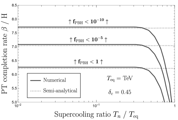
Figure 4: PBH abundance as a function of the amount of supercooling $T_{n}/T_{\rm eq}$ and rate of completion $\beta/H$.

It is convenient to approximate the tunneling rate with the bounce action Taylor-expanded around the nucleation time $t_{n}$ at first order:

$$\Gamma_{{\rm V}}(t)=\Gamma_{0}e^{\beta t}\,\qquad\text{with}\quad\Gamma_{0}=H^{4}(T_{n})e^{-\beta t_{n}}\,,$$ (28)

where the expression for $\Gamma_{0}$ follows from Eq. (27).

During the nucleation phase, the vacuum energy $\Delta V$ is converted into kinetic energy of bubble walls which redshifts akin radiation. The time and position at which a bubble nucleates are stochastic variables. Hence the percolation time of each causal patch fluctuates with respect to the background. While the average universe has already percolated and is cooling like a radiation-dominated universe, late-bloomers – patches which start nucleating later – maintain an almost constant energy density until they finally percolate and convert their vacuum energy into radiation. Hence, causal patches which nucleate the latest inflate the longest and become the densest. Late-blooming region (“late”) collapse into PBHs if the contrast radiation density with respect to the background (“bkg”) is larger than:

$$\delta(t;t_{n_{i}})=\frac{\rho_{\rm R}^{\rm late}(t;t_{n_{i}})-\rho_{\rm R}^{\rm bkg}(t)}{\rho_{\rm R}^{\rm bkg}(t)}\leavevmode\nobreak\ >\leavevmode\nobreak\ \delta_{\rm c}\simeq 0.45,$$ (29)

where $t_{n_{i}}$ is the time at which a late-bloomer nucleates its first bubble. It is also the time until which it remains $100\%$ vacuum-dominated. In presence of bubble growth, the vacuum energy density decreases as:

$$\rho_{V}(t;t_{n_{i}})=F(t;\,t_{n_{i}})\Delta V\,,$$ (30)

where $F(t;\,t_{n_{i}})$ is the volume fraction of remaining false vacuum at time $t$ [151]:

$$F(t;\,t_{n_{i}})=\textrm{exp}\left[-\int_{t_{n_{i}}}^{t}dt{{}^{\prime}}\,\Gamma_{{\rm V}}(t^{{}^{\prime}})a(t{{}^{\prime}})^{3}\frac{4\pi}{3}\left(\int_{t^{{}^{\prime}}}^{t}\frac{d\tilde{t}}{a(\tilde{t})}\right)^{\!\!3}\right],$$ (31)

where $a(t)$ is the scale factor of the universe evolving with energy density $\rho_{\rm tot}=\rho_{\rm V}+\rho_{\rm R}$. Energy-conservation in an expanding universe implies:

$$\dot{\rho}_{\rm R}(t;t_{n_{i}})+4H\rho_{\rm R}(t;t_{n_{i}})=-\dot{\rho}_{V}(t;t_{n_{i}}).$$ (32)

The critical time of nucleation postponing $t_{n_{i}}^{\rm PBH}$ beyond which a causal patch reaches the threshold in Eq. (29) can be found from numerically solving for $\rho_{\rm R}(t;t_{n_{i}})$ in Eq. (32) as a function of $t_{n_{i}}$ for late-bloomers and at $t_{n_{i}}\to 0$ for the background. The fraction $\mathcal{P}_{\rm coll}$ of causal patches which collapse into PBHs is given by the probability that causal patches remain vacuum-dominated until $t_{n_{i}}^{\rm PBH}$. Denoting by $t_{\rm PBH}$ the time when the density contrast reaches the threshold in Eq. (29), we have:

$$\mathcal{P}_{\rm coll}=\exp\left[-\int_{0}^{t_{n_{i}}^{\rm PBH}}dt{{}^{\prime}}\,\Gamma_{{\rm V}}(t{{}^{\prime}})a(t{{}^{\prime}})^{3}V(t^{\prime};t_{\rm PBH})\right]\,,$$ (33)

where $V(t^{\prime};t_{\rm PBH})$ is the comoving volume at time $t^{\prime}$ which is in causal contact with the collapsing patch at $t_{\rm PBH}$:

$$V(t^{\prime};t_{\rm PBH})=\frac{4\pi}{3}\left(r_{\rm H}(t_{\rm PBH})+r(t_{\rm PBH};t{{}^{\prime}})\right)^{3}\,,$$ (34)

with $r_{\rm H}\equiv(aH)^{-1}$ the comoving horizon and $r(t;t^{\prime})=\int_{t^{{}^{\prime}}}^{t}d\tilde{t}/a(\tilde{t})$ the light travel distance between $t^{\prime}$ and $t$.

In Ref. [21], a ready-to-use formula fitted on the numerical calculation is proposed, valid in the supercooled limit $T_{n}\ll T_{\rm eq}$:

$$\mathcal{P}_{\rm coll}\simeq\exp\left[-a\left(\frac{\beta}{H_{n}}\right)^{\!b}\left(1+\delta_{\rm c}\right)^{c\frac{\beta}{H_{n}}}\right]\,,$$ (35)

with $a\simeq 0.5646$, $b\simeq 1.266$, $c\simeq 0.6639$ and $\delta_{c}\simeq 0.45$. Since the collapse occurs during radiation, the PBH mass is given by the mass inside the sound horizon $c_{s}H^{-1}$ at the time of the collapse, e.g. [152]:

$$M_{\rm{PBH}}\simeq M_{\mathMoon}\leavevmode\nobreak\ \left(\frac{106.75}{g_{*}(T_{\rm eq})}\right)^{1/2}\left(\frac{500\leavevmode\nobreak\ \rm GeV}{T_{\rm eq}}\right)^{2},$$ (36)

where $c_{s}=1/\sqrt{3}$ was used and where $M_{\mathMoon}\simeq 3.7\times 10^{-8}M_{\odot}$ is the moon mass. Counting the number of collapsing patches in our past light-cone and weighting them by $M_{\rm{PBH}}$, we obtain the PBH abundance in unit of the DM relic density:

$$f_{\rm{PBH}}\simeq\left(\frac{\mathcal{P}_{\rm coll}}{3.1\times 10^{-12}}\right)\left(\frac{T_{\rm eq}}{1\leavevmode\nobreak\ \rm TeV}\right)\,.$$ (37)

As we show in Fig. 4, values of $\beta/H\lesssim 7$ are needed to produce PBHs in observable abundance $f_{\rm{PBH}}\gtrsim 10^{-5}$.

Appendix B Scale-invariant SM extension

B.1.   SM only

In the SM, the electroweak scale can not be explained by radiative correction alone and a mass scale must be added at tree level. This is because the one-loop contribution to the Higgs potential reads [34]:

$$V(h,T=0)=\frac{\beta_{\lambda_{h}}}{4}h^{4}\left(\ln{\left(\frac{h}{v_{\rm EW}}\right)}-\frac{1}{4}\right),\qquad(4\pi)^{2}\beta_{\lambda_{h}}=\frac{6m_{W}^{4}+3m_{Z}^{4}-12m_{t}^{4}}{v_{\rm EW}^{4}}=-0.035.$$ (38)

Due to the large top mass, the constant $\beta_{\lambda_{h}}<0$ has the wrong sign and $h=0$ is the only minima of the potential.

B.2.   Effective potential

To generate the weak scale with a scale-invariant set-up, we complete the SM with a complex scalar $\Phi=\phi e^{\varphi/\sqrt{2}}$ charged under $U(1)_{\rm D}$. The tree level potential in the unitarity gauge reads:

$$V_{\rm tree}(h,\phi)=\frac{\lambda_{h}}{4}h^{4}+\frac{\lambda_{\phi}}{4}\phi^{4}-\frac{\lambda_{h\phi}}{4}h^{2}\phi^{2}.$$ (39)

The Renormalized Group Equations (RGE) of the theory are given by, e.g. [41]:

$$(4\pi)^{2}\frac{dg_{\rm D}}{d\log{\phi}}=g_{\rm D}^{3}/3,$$ (40)

$$(4\pi)^{2}\frac{d\lambda_{\rm h\phi}}{d\log{\phi}}=\lambda_{h\phi}\left(6y_{t}^{2}+12\lambda_{h}+8\lambda_{\phi}-4\lambda_{\rm h\phi}-6g_{\rm D}^{2}\right),$$ (41)

$$(4\pi)^{2}\frac{d\lambda_{\phi}}{d\log{\phi}}=6g_{\rm D}^{4}+20\lambda_{\phi}^{2}+2\lambda_{hs}^{2}-12\lambda_{\phi}g_{\rm D}^{2}.$$ (42)

Integrating the first equation, we obtain:

$$g_{\rm D}^{2}(\phi)=\frac{g_{\rm D}^{2}(v_{\phi})}{1-\frac{g_{\rm D}^{2}(v_{\phi})}{24\pi^{2}}t},\qquad t\equiv\log\left(\frac{\phi}{v_{\phi}}\right).$$ (43)

The field excursion $\phi_{*}$ during tunneling is of the order of the nucleation temperature $\phi_{*}\sim T_{n}$, see Eq. (63) below. The interval $1\lesssim T_{n}/v_{\phi}\lesssim 10^{-10}$ characteristic of supercooled phase transition implies $-23\lesssim t\lesssim 0$. Hence, we can safely neglect the running of $g_{\rm D}$:

$$t\ll\frac{24\pi^{2}}{g_{\rm D}^{2}}\simeq 950\left(\frac{0.5}{g_{\rm D}}\right)^{2}\qquad\implies\qquad g_{\rm D}(\phi)\simeq g_{\rm D}(v_{\phi}).$$ (44)

Due to collider bounds, the Higgs-mixing is small $\lambda_{h\phi}\lesssim 10^{-2}$, cf. Eq. (8), so we can safely neglect its RGE running in Eq. (41). The integration of Eq. (42) gives:

$$\lambda_{\phi}(\phi)=\frac{3g_{\rm D}^{2}}{10}+\frac{\sqrt{21g_{\rm D}^{4}+10\lambda_{h\phi}^{2}}}{10}\tan{\left\{\frac{\sqrt{21g_{\rm D}^{4}+10\lambda_{h\phi}^{2}}}{8\pi^{2}}t-\arctan{\left[\frac{3g_{\rm D}^{2}-10\lambda_{\phi}^{0}}{\sqrt{21g_{\rm D}^{4}+10\lambda_{h\phi}^{2}}}\right]}\right\}},$$ (45)

where $\lambda_{\phi}^{0}\equiv\lambda_{\phi}(v_{\phi})$ is a boundary value. The potential at 1-loop with counterterm $\delta\lambda\phi^{4}/4$ is:

$$V_{\rm 1-loop}^{T=0}(\phi,h)=\frac{\lambda_{h}}{4}h^{4}-\frac{\lambda_{h\phi}}{4}h^{2}\phi^{2}+\delta\lambda\,\phi^{4}+\frac{\lambda_{\phi}(\phi)}{4}\phi^{4}.$$ (46)

We impose the renormalization condition that $\phi=v_{\phi}$ is the minimum of the potential:

$$\frac{\partial}{\partial\phi}\left[\delta\lambda\,\phi^{4}+\frac{\lambda_{\phi}(\phi)}{4}\phi^{4}\right]_{\phi=v_{\phi}}=0,$$ (47)

which leads to:

$$\delta\lambda=\frac{-3g_{\rm D}^{4}-\lambda_{h\phi}^{2}+6g_{\rm D}^{2}\lambda_{\phi}^{0}-32\pi^{2}\lambda^{0}_{\phi}-10(\lambda_{\phi}^{0})^{2}}{128\pi^{2}}.$$ (48)

Plugging Eqs. (45) and (48) into Eq. (46) and Taylor-expanding as a function of the logarithm $t$, we obtain:

$$V_{\rm 1-loop}^{T=0}(\phi,h)=\frac{\lambda_{h}}{4}h^{4}-\frac{\lambda_{h\phi}}{2}h^{2}\phi^{2}+\frac{\beta_{\lambda}}{4}\phi^{4}\left[\ln{\left(\frac{\phi}{v_{\phi}}\right)}-\frac{1}{4}\right]+\frac{\kappa_{\lambda}}{4}\phi^{4}\ln^{2}{\left(\frac{\phi}{v_{\phi}}\right)}+\cdots,$$ (49)

with:

$$\beta_{\lambda}=\frac{1}{(4\pi)^{2}}\left[6g_{\rm D}^{4}+20(\lambda_{\phi}^{0})^{2}+2\lambda_{h\phi}^{2}-12\lambda_{\phi}^{0}g_{\rm D}^{2}\right]\simeq 6\alpha_{\rm D}^{2},$$ (50)

$$\kappa_{\lambda}=\frac{1}{(4\pi)^{4}}\left[-36g_{\rm D}^{6}+192g_{\rm D}^{4}\lambda_{\phi}^{0}-360g_{\rm D}^{2}(\lambda_{\phi}^{0})^{2}+400(\lambda_{\phi}^{0})^{3}-12g_{\rm D}^{2}\lambda_{h\phi}^{2}+40\lambda_{\phi}^{0}\lambda_{h\phi}^{2}\right]\simeq-\frac{9\alpha_{\rm D}^{3}}{\pi},$$ (51)

where the two right-hand sides assume $g_{\rm D}^{2}\gtrsim\lambda_{\phi}^{0},\lambda_{h\phi}$. We conclude that we can safely truncate the quantum loop correction to first-order in $t$ (leading-log approximation) as long as:

$$t\leavevmode\nobreak\ \ll\leavevmode\nobreak\ \frac{8\pi^{2}}{3g_{\rm D}^{2}}\simeq 105\left(\frac{0.5}{g_{\rm D}}\right)^{2}\quad\implies\quad\kappa_{\lambda}\to 0.$$ (52)

In this study, to minimize the number of parameters, we assume $\lambda_{\phi}^{0}=\lambda_{\phi}(v_{\phi})\ll\sqrt{g_{\rm D}}$, which in practice leads us to set $\lambda_{\phi}^{0}=0$. Instead, despite its small value given by Eq. (8), we keep $\lambda_{h\phi}$ finite in our equations.

Computing the second derivative of the potential around its minimum, we get the scalar mass which is loop-suppressed with respect to the vector boson mass:

$$m_{\phi}^{2}=\beta_{\lambda}v_{\phi}^{2},\qquad\textrm{and}\qquad m_{V}^{2}=g_{\rm D}^{2}v_{\phi}^{2}.$$ (53)

The total potential is given by:

$$V(\phi)=\frac{\lambda_{\phi}(\phi)}{4}\phi^{4}+V_{\rm T}(\phi)+V_{\rm QCD}(\phi).$$ (54)

The second piece contains the finite temperature correction at one loop and the Daisy contributions which accounts for the resummation of the Matsubara zero modes [68]:

$$V_{\rm T}(\phi)=\frac{T^{4}}{2\pi^{2}}J_{B}\left(\frac{m_{V}^{2}(\phi)}{T^{2}}\right)+\frac{T}{12\pi}\left[m_{V}^{3}-\left(m_{V}^{2}+\Pi_{V}\right)^{3/2}\right],$$ (55)

with vacuum and thermal masses $m_{V}^{2}(\phi)=g_{\rm D}^{2}\phi^{2}$ and $\Pi_{V}=g_{\rm D}^{2}T^{2}/6$ respectively [69]. The third piece contains the Higgs contribution below the temperature of QCD confinement, see main text

$$V_{\rm QCD}(\phi)=-\frac{1}{2}m_{{\rm QCD}}^{2}\phi^{2},\qquad\textrm{with}\quad m_{{\rm QCD}}^{2}=\frac{1}{2}\lambda_{h\phi}\left<h\right>_{{\rm QCD}}^{2}\Theta(T-\Lambda_{\rm QCD}).$$ (56)

B.3.   Bounce action

The cost for nucleating a bubble through thermal tunneling is given by the action [77]

$$\frac{S_{3}}{T}=\frac{4\pi}{T}\int dr\,r^{2}\left[\frac{1}{2}\phi^{{}^{\prime}}(r)^{2}+V(\phi)\right],$$ (57)

where the tunneling trajectory reads

$$\phi^{{}^{\prime\prime}}(r)+\frac{2}{r}\phi^{{}^{\prime}}(r)=\frac{dV}{d\phi},\quad\phi^{{}^{\prime}}(0)=0,\quad\underset{r\to\infty}{\textrm{lim}}\,\phi(r)=0.$$ (58)

We calculate the bounce action $S_{3}$ in Eq. (57) both numerically and analytically.

Numerical method — We wrote an over-shooting/under-shooting C++ software program ${\tt CCBounce}$ [49] using the full potential in Eq. (54) and the quartic coupling being given by Eq. (45). We checked that the error is below the percent level as explained in [80, chap. 6]. Results are shown with thick lines in Fig. 5.

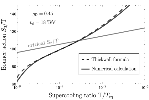
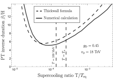
Figure 5: Bounce action $S_{3}/T$ (left) and rate $\beta/H$ of the phase transition (right). The thickwall analytical formula is a good approximation of the numerical results.

Thick-wall method — We numerically find that the field value $\phi_{*}$ at the center of a nucleated bubble is of the order of the temperature $\phi_{*}\sim T_{n}\ll v_{\phi}$. This allows two approximation schemes. First of all, we can Taylor-expand the potential $V(\phi)=V_{T=0}+V_{\rm T}+V_{{\rm QCD}}$ at first order in $\phi/T\ll 1$:

$$V(\phi)\simeq\frac{m_{\rm eff}^{2}(T)}{2}\phi^{2}-\frac{\lambda_{\rm eff}}{4}\phi^{4}$$ (59)

with

$$m_{\rm eff}^{2}(T)\simeq\frac{1}{12}\,g_{\rm D}^{2}\,T^{2}-m_{{\rm QCD}}^{2},\qquad\lambda_{\rm eff}\simeq\beta_{\lambda}\,\ln{\frac{e^{1/4}v_{\phi}}{\phi}}.$$ (60)

Second of all, we can use the thick-wall formula [79], see for instance the textbook [80, chap. 6]:

$$\frac{S_{3}}{T}=\frac{16\pi}{3\,\lambda_{\rm eff}}\frac{m_{\rm eff}}{T},\qquad\text{and}\qquad\phi_{*}=2\frac{m_{\rm eff}}{\sqrt{-\lambda_{\rm eff}}}.$$ (61)

In terms of the physical parameters, $S_{3}$ becomes:

$$\frac{S_{3}}{T}\simeq\frac{A}{\textrm{log}\left(\frac{M}{T}\right)}\quad\text{with}\quad M=0.43\,g_{\rm D}\,v_{\phi},\quad$$ (62)

$$A=\frac{127.3}{g_{\rm D}^{3}}\sqrt{1-\left(\frac{T_{{\rm QCD}}}{T}\right)^{\!2}},\quad T_{{\rm QCD}}=\frac{\sqrt{6\lambda_{\rm h\sigma}}}{g_{\rm D}}\left<h\right>_{{\rm QCD}}.$$

and the field value at the tunneling exit reads:

$$\phi_{*}\simeq\left(\frac{8}{\log{\frac{v_{\phi}}{T}}}\right)^{1/2}\frac{T}{g_{\rm D}}.$$ (63)

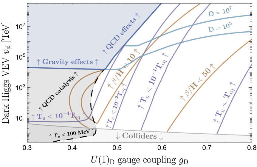
Figure 6: Parameter space of the minimal $U(1)_{\rm D}$ scale-invariant model with large amount of supercooling $T_{n}/T_{\rm eq}<1$ (purple lines) and slow completion rate encoded by $\beta/H$ (orange lines). See Fig. 3 for the rest of the legend.

For consistency, we check that the $O_{4}$-symmetric bounce for quantum tunneling which in the thick-wall limit reads [79, 80]:

$$S_{4}\simeq\frac{2\pi^{2}}{\lambda_{\rm eff}},$$ (64)

is always larger than the $O_{3}$-symmetric bounce in Eq. (61):

$$\frac{S_{3}}{T}\lesssim S_{4}\qquad\rightarrow\qquad m_{\rm eff}\lesssim T\qquad\rightarrow\qquad g_{\rm D}\lesssim 4,$$ (65)

and therefore its contribution to the tunneling can be neglected. Fig. 5 shows that the thick-wall formula compares reasonably well with the numerical formula. We can safely use it in the rest of this work. The nucleation temperature $T_{n}$ and phase transition rate $\beta/H$ are plotted in Fig. 6, and also Fig. 1 of the main text.

Validity of the single-field approximation — Apart from the QCD contribution, in the above discussion we have neglected the motion of the Higgs field $h$ during tunneling of the $U(1)_{\rm D}$ scalar $\phi$. We now check that this is a valid approximation. In the supercooling limit $T_{n}\ll T_{\rm eq}$, the exit point of tunneling $\phi_{*}$ in Eq. (63) is hierarchically small:

$$\phi_{*}\simeq\left(\frac{8}{\ln{\frac{v_{\phi}}{T_{n}}}}\right)^{1/2}\frac{T}{g_{\rm D}}\leavevmode\nobreak\ \ll\leavevmode\nobreak\ v_{\phi}.$$ (66)

The motion of $\phi$ during tunneling does induce a motion of $h$ if the negative induced mass $-\frac{1}{2}\lambda_{h\phi}\phi_{*}^{2}$ is larger than the positive thermal mass $m_{h}^{2}(T)\simeq(\frac{3g_{2}^{2}}{16}+\frac{y_{t}^{2}}{4}+\frac{\lambda_{h}}{2})T^{2}$ which implies:

$$g_{\rm D}\leavevmode\nobreak\ <\leavevmode\nobreak\ 0.4\left(\frac{8}{\ln{\frac{v_{\phi}}{T_{n}}}}\right)^{1/2}\frac{0.4\leavevmode\nobreak\ \rm TeV}{v_{\phi}}.$$ (67)

Whenever Eq. (67) is verified, during tunneling the Higgs field acquires the value $h_{\rm exit}\simeq\phi_{*}\sqrt{\lambda_{h\phi}/\lambda_{h}}$. The motion of $h$ backreacts on the tunneling if the negative induced mass $-\frac{1}{2}\lambda_{h\phi}h_{\rm exit}^{2}$ is comparable to the thermal mass $m_{\phi}^{2}(T)\simeq g_{\rm D}^{2}T^{2}/12$ which implies:

$$g_{\rm D}\leavevmode\nobreak\ <\leavevmode\nobreak\ 0.8\left(\frac{8}{\ln{\frac{v_{\phi}}{T_{n}}}}\right)^{1/4}\frac{0.4\leavevmode\nobreak\ \rm TeV}{v_{\phi}},$$ (68)

where we used $\lambda_{h\phi}=2\lambda_{h}(v_{\rm EW}/v_{\phi})^{2}$ and $\lambda_{h}\simeq 0.13$, cf. Eq. (8). We conclude that we can safely neglect the motion of the Higgs during tunneling (except for QCD catalysis discussed in the main text).

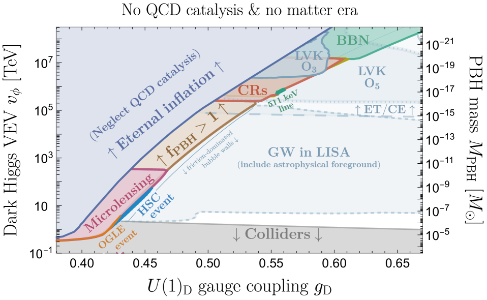
Figure 7: Same as Fig. 3 under the assumption that the QCD catalysis does not arise and that the universe follows an adiabatic evolution after the PT. The later point would arise if the dark scalar decays right after percolation, see e.g. [22]. In contrast to the minimal case presented in the main text, all the regions producing observable PBHs are testable with future GW interometers, above astrophysical foregrounds, including the region explaining DM as made of PBHs. The thin orange region in the bottom-left corner can explain the six ultra-short lensing events observed with OGLE telescopes after five years of observation of the Galactic bulge and which could be attributed to PBHs with masses $10^{-6}M_{\odot}>M_{\rm PBH}>10^{-3}M_{\odot}$ [112, 100]. This region is absent in Fig. 3, which implies that effects from QCD catalysis prevent the scale-invariant EWPT to explain OGLE events.

B.4.   Collider constraints

Mixing angle — Within a view to applying collider bounds to the SM extension we consider, we review the derivation of the mixing angle $\theta_{h\phi}$. The Lagrangian after spontaneous symmetry breaking (with quantum corrections included) reads:

$$\mathcal{L}\supset-\mu_{h}^{2}|H|^{2}-\lambda_{h}|H|^{4}-\mu_{\phi}|\Phi|^{2}-\lambda_{\phi}|\Phi|^{4}-\lambda_{h\phi}|\Phi|^{2}|H|^{2},$$ (69)

with $H=\left(0,\frac{v_{\rm EW}+\tilde{h}}{\sqrt{2}}\right)$ and $\Phi=\frac{v_{\phi}+\tilde{\phi}}{\sqrt{2}}$ the gauge eigenstates. The minimum of the potential at $(v_{\phi},\,v_{\rm EW})$ implies:

$$\mu_{h}^{2}=-\lambda_{h}v_{\rm EW}^{2}-\frac{1}{2}\lambda_{h\phi}v_{\phi}^{2},\quad\mu_{\phi}^{2}=-\lambda_{\phi}v_{\phi}^{2}-\frac{1}{2}\lambda_{h\phi}v_{\rm EW}^{2},\qquad v_{\rm EW}\simeq 246\leavevmode\nobreak\ \rm GeV.$$ (70)

The mixing angle $\theta_{h\phi}$ is defined as the rotation angle between the gauge eigenstates and the mass eigenstates:

$$\left(\begin{array}[]{c}h\\ \phi\end{array}\right)=\left(\begin{array}[]{cc}\cos{\theta_{h\phi}}&\sin{\theta_{h\phi}}\\ -\sin{\theta_{h\phi}}&\cos{\theta_{h\phi}}\end{array}\right)\left(\begin{array}[]{c}\tilde{h}\\ \tilde{\phi}\end{array}\right),$$ (71)

with associated mass eigenvalues:

$$m_{h}^{2}=2\lambda_{h}v_{\rm EW}^{2}\cos^{2}{\theta_{h\phi}}+2\lambda_{\phi}v_{\phi}^{2}\sin^{2}{\theta_{h\phi}}-\lambda_{h\phi}v_{\phi}v_{\rm EW}\sin{2\theta_{h\phi}},$$ (72)

$$m_{\phi}^{2}=2\lambda_{h}v_{\rm EW}^{2}\sin^{2}{\theta_{h\phi}}+2\lambda_{\phi}v_{\phi}^{2}\cos^{2}{\theta_{h\phi}}+\lambda_{h\phi}v_{\phi}v_{\rm EW}\sin{2\theta_{h\phi}}.$$ (73)

We find:

$$\sin{2\theta_{h\phi}} =\frac{\lambda_{h\phi}v_{\phi}v_{\rm EW}}{\sqrt{((\lambda_{\phi}v_{\phi}^{2}-\lambda_{h}v_{\rm EW}^{2})^{2}+(\lambda_{h\phi}v_{\phi}v_{\rm EW})^{2}}},$$ (74)

where $\lambda_{h\phi}=(m_{h}/v_{\phi})^{2}$, $\lambda_{h}=m_{h}^{2}/2v_{\rm EW}^{2}$ and $\lambda_{\phi}=11\beta_{\lambda}/6$.

Higgs searches — We use Eq. (74) to recast existing collider constraints on additional Higgs boson on the parameter space of the minimal scale-invariant $U(1)_{\rm D}$ extension of the SM, see Fig. 8. For $g_{\rm D}\sim 0.5$, we find that the tightest constraints are given by LEP searches $v_{\phi}\gtrsim 1.5\leavevmode\nobreak\ \rm TeV$, the mass of the dark Higgs being $m_{\phi}\gtrsim 80\leavevmode\nobreak\ \rm GeV$.

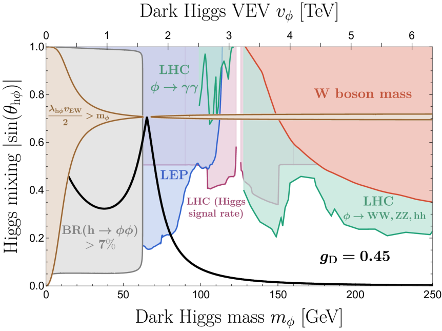
Figure 8: Collider constraints on mixing angle $\theta_{h\phi}$ in scale-invariant $U(1)_{\rm D}$ extension of the SM (black line) as a function of the extra Higgs mass $m_{\phi}$. We show LEP searches for 4-fermion final states from Higgs strahlung $e^{+}e^{-}\to Z\phi$ [108] (blue), resonant production at LHC [109] (green), electroweak fit of the W mass [109] (red), Higgs signal shape [110] (purple), Higgs decay to new particle [111] (gray). In the brown region, the scalar mass $m_{\phi}$ is induced by the Higgs VEV.

Appendix C Bubble dynamics

C.1.   Energy budget

The motion of bubble walls is subject to the driving vacuum pressure $\Delta V$ and to the retarding friction pressure which after resumming leading-logs quantum corrections (LL) reads [81, 82, 83, 84]:

$$\mathcal{P}_{\rm LL}=c_{0}\,g_{\rm D}^{3}\gamma v_{\phi}T_{n}^{3}\log\left(\frac{v_{\phi}}{T_{n}}\right),\qquad c_{0}=\mathcal{O}(1),$$ (75)

where $\gamma$ is the bubble wall Lorentz factor. We suppose the leading-order pressure $\mathcal{P}_{\rm LO}$ to be sub-dominant since it does not grow with $\gamma$ [153]. In the absence of friction $\mathcal{P}_{\rm LL}\ll\Delta V$, all the vacuum energy $E_{\rm vac}=4\pi R^{3}\Delta V/3$ of a bubble of radius $R$ is converted into kinetic energy of the wall $E_{\rm wall}=4\pi R^{2}\sigma\gamma$, where $\sigma$ is the wall surface tension. In that case, the wall Lorentz factor at collision reaches the maximal value allowed by energy conservation:

$$\gamma_{\rm max}=\frac{\Delta VR_{\rm coll}}{3\sigma}=\frac{2R_{\rm coll}}{3R_{\rm crit}}.$$ (76)

The mean bubble radius at collision is given by $R_{\rm coll}\simeq\pi^{1/3}/\beta$ [154]. We introduced $R_{\rm crit}=2\sigma/\Delta V$ which is the critical radius for nucleating a bubble, found as the saddle point of the free energy $F(R)=4\pi\sigma R^{2}-4\pi R^{3}\Delta V/3$ in the thin-wall approximation. As bubble walls accelerate, the retarding pressure $\mathcal{P}_{\rm LL}$ in Eq. (75) grows linearly with $\gamma$. The walls stops accelerating as soon as $\mathcal{P}_{\rm LL}\simeq\Delta V$, with the associated Lorentz factor:

$$\gamma_{\rm LL}\simeq\frac{\Delta V}{c_{0}\,g_{\rm D}^{3}\gamma v_{\phi}T_{n}^{3}\log\left(\frac{v_{\phi}}{T_{n}}\right)}.$$ (77)

Whether the latent heat of the PT is dominantly converted into the plasma or into the kinetic energy of the wall depends on whether Eq. (76) or (77) dominate. The Lorentz factor at bubble collision is given by the formula:

$$\gamma_{\rm coll}=\textrm{Min}\left[\gamma_{\rm max},\leavevmode\nobreak\ \gamma_{\rm LL}\right].$$ (78)

The fraction of the latent heat converted into wall kinetic energy reads (see also [155]):

$$\kappa_{\rm coll}=\frac{E_{\rm wall}}{E_{\rm vac}}=\frac{3\gamma\sigma R_{\rm coll}}{\Delta V}=\frac{\gamma_{\rm coll}}{\gamma_{\rm max}}.$$ (79)

C.2.   Reheating after a matter era

At the time of bubble percolation, the latent heat of the universe has been converted into two fluids, the radiation-like energy density $\rho_{\rm shock}$ of the ultra-relativistic shock waves generated by the work of the friction pressure, and the radiation-like energy density of the scalar field gradient $\rho_{\rm\phi}$. Both are highly peaked distribution of energy-momentum tensor. After that walls pass through each other, the highly peaked energy stored in the wall $E_{\rm wall}\simeq\gamma_{\rm coll}\sigma R_{\rm coll}^{2}$ is converted into a broadly-distributed oscillating scalar field condensate with energy $E_{\rm osc}\simeq\Delta VR_{\rm coll}^{2}\Delta R$ where $\Delta R$ is the distance between the two peaks in energy-momentum tensor after their collision. The radiation-like energy stored in the collided walls is converted into the matter-like oscillating scalar condensate $E_{\rm wall}=E_{\rm osc}$ after the time:

$$\Delta R_{\rm max}\simeq\frac{\sigma\gamma_{\rm coll}}{\Delta V}\simeq\frac{\gamma_{\rm coll}}{\gamma_{\rm max}}R_{\rm coll}\simeq\kappa_{\rm coll}R_{\rm coll}.$$ (80)

If the scalar field is long-lived $\Gamma_{\phi}\ll H$, then the scalar field energy density starts redshifting like matter with an energy density after percolation given by:

$$\rho_{\rm M}(t)=\kappa_{\rm coll}\Delta V\left(\frac{a(t_{n})}{a(t)}\right)^{3}.$$ (81)

The radiation energy density reads:

$$\rho_{\rm R}(t)=(1-\kappa_{\rm coll})\Delta V\left(\frac{a(t_{n})}{a(t)}\right)^{4}.$$ (82)

The scalar field decays after the time approximately given by its inverse decay width:

$$t_{\rm dec}\simeq\Gamma_{\phi}^{-1},\quad\implies\quad T_{\rm dec}=\frac{1.2}{g_{*}^{1/4}}\sqrt{M_{\rm pl}\Gamma_{\phi}},$$ (83)

where we also gave the associated temperature. If long-lived enough, this would lead to a matter-domination era starting at the time and temperature:

$$t_{\rm dom}\simeq t_{n}/\kappa_{\rm coll}^{2}\quad\implies\quad T_{\rm dom}\simeq\kappa_{\rm coll}T_{\rm eq},$$ (84)

obtained from equating Eqs. (81) and (82) with $a\propto t^{1/2}$. We conclude that if $t_{\rm dom}<t_{\rm dec}$ then the PT is followed by a matter era starting at $t_{\rm dom}$ and ending at $t_{\rm dec}$. A transition from a matter to radiation inject an amount of entropy in the universe, e.g. [156, 157, 158], whose magnitude is given by the dilution factor:

$$D\equiv\frac{S_{f}}{S_{i}}=1+\frac{T_{\rm dom}}{T_{\rm dec}},$$ (85)

where $S_{i}$ and $S_{f}$ is the total entropy in the universe just before and just after the decay of the scalar field, assuming an instantaneous decay. The second equality comes from evolving matter and radiation from $T_{\rm dom}$ to $T_{\rm dec}$. The entropy injection dilutes the abundance of any relic present in the universe before $t_{\rm dom}$. This is the case of PBHs and GWs. For PBHs, the abundance is simply rescaled by:

$$f_{\rm PBH}\rightarrow\frac{f_{\rm PBH}}{D}.$$ (86)

For GWs, the spectrum is rescaled by:

$$\Omega_{\rm GW}(f)\rightarrow\frac{\Omega_{\rm GW}(D^{1/3}f)}{D^{4/3}}S_{M}(f).$$ (87)

where the $D$ factors trivially correct for the redshift of the peak amplitude and frequency [136]. Instead, the effects behind $S_{M}(f)$ are more subtle and consist to change the spectral slope to $\propto f^{1}$ [132, 133, 134, 135] instead of $f^{3}$ [159, 160, 161] for modes with wavenumber $k=2\pi f$ which are super-horizon $k<H_{n}/a$ at percolation and enter the causal horizon $k=H/a$ during the matter era. In other words, $S_{M}(f)$ is designed to change the spectral slope to:

$$\Omega_{\rm GW}(f)S_{M}(f)\propto f^{1}\qquad\textrm{for}\qquad f_{\rm dec}<f<f_{\rm dom},$$ (88)

assuming continuity with the standard spectrum at $f_{\rm dom}$. We have introduced the frequencies corresponding to the causal horizon $H/2\pi$ at the beginning and end of the matter era red-shifted up to today:

$$f_{\rm dom}=\left(\frac{a_{\rm dom}}{a_{0}}\right)\frac{H_{\rm dom}}{2\pi},$$ (89)

$$f_{\rm dec}=\left(\frac{a_{\rm dec}}{a_{0}}\right)\frac{H_{\rm dec}}{2\pi},$$ (90)

with $H\simeq 0.3g_{*}^{1/2}T^{2}/M_{\rm pl}$ given by Friedman’s equation and:

$$\frac{a_{\rm dom}}{a_{0}}=\frac{1.65\times 10^{-2}\leavevmode\nobreak\ {\rm mHz}}{D^{1/3}}\leavevmode\nobreak\ \left(\frac{T_{\rm dom}}{100\leavevmode\nobreak\ \rm GeV}\right)\left(\frac{g_{*}(T_{\rm dom})}{100}\right)^{1/6}H_{\rm dom}^{-1},$$ (91)

$$\frac{a_{\rm dec}}{a_{0}}=1.65\times 10^{-2}\leavevmode\nobreak\ {\rm mHz}\leavevmode\nobreak\ \left(\frac{T_{\rm dec}}{100\leavevmode\nobreak\ \rm GeV}\right)\left(\frac{g_{*}(T_{\rm dec})}{100}\right)^{1/6}H_{\rm dec}^{-1},$$ (92)

where the dilution factor $D$ is only applied to $f_{\rm dom}$. The GW spectrum $\Omega_{\rm GW}(f)$ from bubble dynamics is presented in the next section.

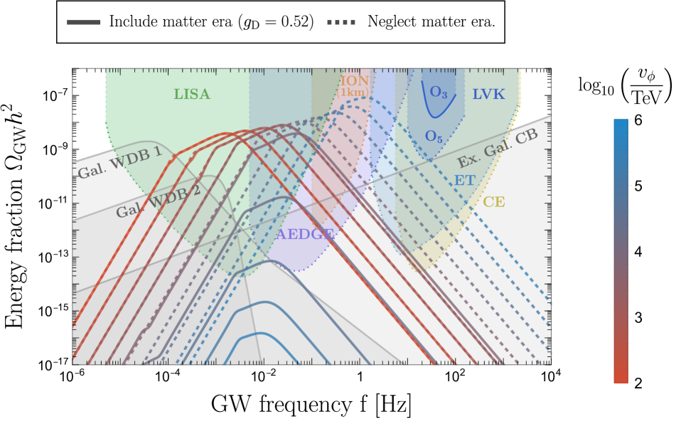
Figure 9: Gravitational waves spectrum produced by the supercooled first-order phase transition predicted in the minimal $U(1)_{\rm D}$ extension of the SM. Solid lines shows the GW spectra accounting for the matter-dominated period after the PT, which suppresses the signal at large dark Higgs VEV $v_{\phi}\gtrsim 10^{4}\leavevmode\nobreak\ \rm TeV$. In comparison, dotted lines show the same GW spectra without the matter era. The colorful regions show the existing constraints from Earth-based laser interometers LIGO-Virgo-Kagra (LVK) run O3 [86], assuming Signal-to-Noise Ratio (SNR) detection thresholds of 2, and prospective constraints from LIGO run $O_{5}$ [87], their follow-ups Einstein Telescope (ET) [88, 89] and Cosmic Explorer (CE) [90], space-based laser interferometer LISA [91, 92, 93], Earth-based atom interferometer AION [162, 163] in its space version AEDGE [164]. For LISA, ET and CE, we optimistically assume a low SNR threshold of 1 (equivalent to a 1$\sigma$ deviation from noise) after 20 years of observation [165]. The gray regions show the expected astrophysical foreground from galactic white dwarf binaries (WD B.) according to model 1 [95, 96] and 2 [92], and extragalactic compact (neutron stars and black holes) binaries (Compact B.) fitted on LIGO O3 data [86]. Instead, the contribution from extragalactic supermassive black holes binaries lies at lower frequencies [97]. All the GW constraints in Figs. 2, 3, and 7 are derived assuming that the GW spectra is above the astrophysical foregrounds inside the frequency window of experiments.

C.3.   GW signal

Scalar field gradient — A fraction $\kappa_{\rm coll}$ given by Eq. (79) of the latent heat is stored in the scalar field gradient localised in bubble walls. Initially, the GW spectrum has been calculated in the “envelop” approximation where walls are infinitely thin and collided parts are removed from the calculation [166, 167, 168, 169, 170]. The collided part were studied later both analytically [120] and numerically [121, 122, 123, 124] in what is known as the “bulk flow” model. It is found that the collided part continue to source GW after collision, generating the slow decreasing IR slope $\Omega_{\rm GW}\propto f^{1}$. The GW spectrum in the bulk flow model gives ($v_{w}=1$) [121]:

$$\Omega_{\rm GW}h^{2}\simeq\frac{1}{D^{4/3}}\frac{10^{-6}}{(g_{*}/100)^{1/3}}\left(\frac{H_{n}}{\beta}\right)^{\!2}\left(\frac{\alpha}{1+\alpha}\right)^{\!2}S(f)S_{H}(f)S_{M}(f),$$ (93)

with the redshift factor between percolation “$n$” and today “$0$”:

$$a_{n}/a_{0}=\frac{1.65\times 10^{-2}\leavevmode\nobreak\ {\rm mHz}}{D^{1/3}}\leavevmode\nobreak\ \left(\frac{T_{\rm eq}}{100\leavevmode\nobreak\ \rm GeV}\right)\left(\frac{g_{*}(T_{\rm eq})}{100}\right)^{1/6}H_{n}^{-1},$$ (94)

and the spectral shape $S(f)$ peaking on $f_{p}$:

$$S(f)=\frac{3(f/f_{\rm p})^{0.9}}{2.1+0.9(f/f_{\rm p})^{3}},\quad f_{\rm p}=\left(\frac{a_{n}}{a_{0}}\right)0.8\left(\frac{\beta}{2\pi}\right).$$ (95)

The dilution factor $D\geq 1$ given by Eq. (85) accounts for the additional redshift due to entropy injection in presence of an eventual early matter era if the scalar $\phi$ is long-lived. We added the correction factor:

$$S_{H}(f)=\frac{(f/f_{H})^{2.1}}{1+(f/f_{H})^{2.1}},\quad f_{H}=c_{*}\left(\frac{a_{n}}{a_{0}}\right)\left(\frac{H_{n}}{2\pi}\right),$$ (96)

with $c_{*}=\mathcal{O}(1)$ to impose the scaling $\Omega_{\rm GW}\propto f^{3}$ for emitted frequencies smaller than the Hubble factor $H_{\ast}/(2\pi)$ and entering during radiation [159, 160, 161, 135]. We set $c_{*}=1$ and defer the determination of $c_{*}$ for future studies, see e.g. [171, 172]. The factor $S_{\rm M}(f)$ corrects the causality tail $f^{3}\to f^{1}$ for modes entering during the matter era instead of the radiation era, as explained in Eq. (88).

Ultrarelativistic shells — We know discuss GW generation from the fraction $1-\kappa_{\rm coll}$ of latent heat stored in terms of fluid motions. In the ultra-relativistic limit, one expects bubble walls to be followed by ultra relativistic shells of particles which are generated by plasma/wall interactions [117, 113, 82, 83, 114, 115, 115, 84] which are extremely thin [113] and whose impact on the GW spectrum is not yet understood [118, 119] at the time of writing. Waiting for future studies to investigate the precise GW spectrum from ultrarelativistic shells, we posit that from the point of view of gravity, the GW production from extremely thin shells of scalar field gradient should be indistinguishable from extremely thin shells of ultra-relativistic particles. A difference could arise however due to ultra-relativistic shocks being potentially long-lived [117] while scalar field gradient having a reduced lifetime given by Eq. (80). One expect such difference to enhance the GW spectrum by a factor $\beta/H$. Since this is a small factor in the regime of interest for PBH production, we do not include it in our plot. However, we checked that the conclusion of this paper do not depend on this detail.

Hence, we suppose that the bulk flow model holds in all the parameter space. However, the friction still has an important impact on the GW spectrum through the dependence of the dilution factor on the latent heat fraction into scalar field gradient, see Eqs. (85), (84) and (79). We show a family of GW spectrum for different values of PT scale $v_{\phi}$ in Fig. 9 together with LISA reach and astrophysical foregrounds. The constraints on the scale invariant $U(1)_{\rm D}$ extension of the SM are shown in Figs. 3, 2 and 7. For large dark Higgs VEV $v_{\phi}\gtrsim 10^{4}\leavevmode\nobreak\ \rm TeV$, the extended dark Higgs lifetime generates entropy injection and suppresses all GW signals, leaving PBHs as the only possible signatures.

References

- Abbott et al. [2021a] R. Abbott et al. (LIGO Scientific, VIRGO, KAGRA), GWTC-3: Compact Binary Coalescences Observed by LIGO and Virgo During the Second Part of the Third Observing Run, (2021a), arXiv:2111.03606 [gr-qc] .
- Agazie et al. [2023] G. Agazie et al. (NANOGrav), The NANOGrav 15 yr Data Set: Evidence for a Gravitational-wave Background, Astrophys. J. Lett. 951, L8 (2023), arXiv:2306.16213 [astro-ph.HE] .
- Antoniadis et al. [2023] J. Antoniadis et al. (EPTA, InPTA:), The second data release from the European Pulsar Timing Array - III. Search for gravitational wave signals, Astron. Astrophys. 678, A50 (2023), arXiv:2306.16214 [astro-ph.HE] .
- Reardon et al. [2023] D. J. Reardon et al., Search for an Isotropic Gravitational-wave Background with the Parkes Pulsar Timing Array, Astrophys. J. Lett. 951, L6 (2023), arXiv:2306.16215 [astro-ph.HE] .
- Carr and Hawking [1974] B. J. Carr and S. W. Hawking, Black holes in the early Universe, Mon. Not. Roy. Astron. Soc. 168, 399 (1974).
- Carr et al. [2016] B. Carr, F. Kuhnel, and M. Sandstad, Primordial Black Holes as Dark Matter, Phys. Rev. D 94, 083504 (2016), arXiv:1607.06077 [astro-ph.CO] .
- Carr and Kuhnel [2020] B. Carr and F. Kuhnel, Primordial Black Holes as Dark Matter: Recent Developments, Ann. Rev. Nucl. Part. Sci. 70, 355 (2020), arXiv:2006.02838 [astro-ph.CO] .
- Carr et al. [2021] B. Carr, K. Kohri, Y. Sendouda, and J. Yokoyama, Constraints on primordial black holes, Rept. Prog. Phys. 84, 116902 (2021), arXiv:2002.12778 [astro-ph.CO] .
- Green and Kavanagh [2021] A. M. Green and B. J. Kavanagh, Primordial Black Holes as a dark matter candidate, J. Phys. G 48, 043001 (2021), arXiv:2007.10722 [astro-ph.CO] .
- Sato et al. [1981] K. Sato, M. Sasaki, H. Kodama, and K.-i. Maeda, Creation of Wormholes by First Order Phase Transition of a Vacuum in the Early Universe, Prog. Theor. Phys. 65, 1443 (1981).
- Maeda et al. [1982] K.-i. Maeda, K. Sato, M. Sasaki, and H. Kodama, Creation of De Sitter-schwarzschild Wormholes by a Cosmological First Order Phase Transition, Phys. Lett. B 108, 98 (1982).
- Sato et al. [1982] K. Sato, H. Kodama, M. Sasaki, and K.-i. Maeda, Multiproduction of Universes by First Order Phase Transition of a Vacuum, Phys. Lett. B 108, 103 (1982).
- Kodama et al. [1981] H. Kodama, M. Sasaki, K. Sato, and K.-i. Maeda, Fate of Wormholes Created by First Order Phase Transition in the Early Universe, Prog. Theor. Phys. 66, 2052 (1981).
- Kodama et al. [1982] H. Kodama, M. Sasaki, and K. Sato, Abundance of Primordial Holes Produced by Cosmological First Order Phase Transition, Prog. Theor. Phys. 68, 1979 (1982).
- Hsu [1990] S. D. H. Hsu, Black Holes From Extended Inflation, Phys. Lett. B 251, 343 (1990).
- Liu et al. [2022] J. Liu, L. Bian, R.-G. Cai, Z.-K. Guo, and S.-J. Wang, Primordial Black Hole Production during First-Order Phase Transitions, Phys. Rev. D 105, L021303 (2022), arXiv:2106.05637 [astro-ph.CO] .
- Hashino et al. [2021] K. Hashino, S. Kanemura, and T. Takahashi, Primordial Black Holes as a Probe of Strongly First-Order Electroweak Phase Transition, (2021), arXiv:2111.13099 [hep-ph] .
- He et al. [2022] S. He, L. Li, Z. Li, and S.-J. Wang, Gravitational Waves and Primordial Black Hole Productions from Gluodynamics, (2022), arXiv:2210.14094 [hep-ph] .
- Kawana et al. [2022] K. Kawana, T. Kim, and P. Lu, PBH Formation from Overdensities in Delayed Vacuum Transitions, (2022), arXiv:2212.14037 [astro-ph.CO] .
- Lewicki et al. [2023] M. Lewicki, P. Toczek, and V. Vaskonen, Primordial black holes from strong first-order phase transitions, JHEP 09, 092, arXiv:2305.04924 [astro-ph.CO] .
- Gouttenoire and Volansky [2023] Y. Gouttenoire and T. Volansky, Primordial Black Holes from Supercooled Phase Transitions, (2023), arXiv:2305.04942 [hep-ph] .
- Baldes and Olea-Romacho [2023] I. Baldes and M. O. Olea-Romacho, Primordial black holes as dark matter: Interferometric tests of phase transition origin, (2023), arXiv:2307.11639 [hep-ph] .
- Salvio [2023] A. Salvio, Supercooling in Radiative Symmetry Breaking: Theory Extensions, Gravitational Wave Detection and Primordial Black Holes, (2023), arXiv:2307.04694 [hep-ph] .
- Banerjee and Dey [2023] I. K. Banerjee and U. K. Dey, Spinning Primordial Black Holes from First Order Phase Transition, (2023), arXiv:2311.03406 [gr-qc] .
- Gehrman et al. [2023] T. C. Gehrman, B. Shams Es Haghi, K. Sinha, and T. Xu, The Primordial Black Holes that Disappeared: Connections to Dark Matter and MHz-GHz Gravitational Waves, (2023), arXiv:2304.09194 [hep-ph] .
- Afzal et al. [2023] A. Afzal et al. (NANOGrav), The NANOGrav 15 yr Data Set: Search for Signals from New Physics, Astrophys. J. Lett. 951, L11 (2023), arXiv:2306.16219 [astro-ph.HE] .
- Gouttenoire [2023a] Y. Gouttenoire, First-Order Phase Transition Interpretation of Pulsar Timing Array Signal Is Consistent with Solar-Mass Black Holes, Phys. Rev. Lett. 131, 171404 (2023a), arXiv:2307.04239 [hep-ph] .
- He et al. [2023] S. He, L. Li, S. Wang, and S.-J. Wang, Constraints on holographic QCD phase transitions from PTA observations, (2023), arXiv:2308.07257 [hep-ph] .
- Ellis et al. [2023] J. Ellis, M. Fairbairn, G. Franciolini, G. Hütsi, A. Iovino, M. Lewicki, M. Raidal, J. Urrutia, V. Vaskonen, and H. Veermäe, What is the source of the PTA GW signal?, (2023), arXiv:2308.08546 [astro-ph.CO] .
- Aad et al. [2012] G. Aad et al. (ATLAS), Observation of a new particle in the search for the Standard Model Higgs boson with the ATLAS detector at the LHC, Phys. Lett. B 716, 1 (2012), arXiv:1207.7214 [hep-ex] .
- Chatrchyan et al. [2012] S. Chatrchyan et al. (CMS), Observation of a New Boson at a Mass of 125 GeV with the CMS Experiment at the LHC, Phys. Lett. B 716, 30 (2012), arXiv:1207.7235 [hep-ex] .
- Salam et al. [2022] G. P. Salam, L.-T. Wang, and G. Zanderighi, The Higgs boson turns ten, Nature 607, 41 (2022), arXiv:2207.00478 [hep-ph] .
- Gildener and Weinberg [1976] E. Gildener and S. Weinberg, Symmetry Breaking and Scalar Bosons, Phys. Rev. D 13, 3333 (1976).
- Coleman and Weinberg [1973] S. R. Coleman and E. J. Weinberg, Radiative Corrections as the Origin of Spontaneous Symmetry Breaking, Phys. Rev. D 7, 1888 (1973).
- Hempfling [1996] R. Hempfling, The Next-To-Minimal Coleman-Weinberg Model, Phys. Lett. B 379, 153 (1996), arXiv:hep-ph/9604278 .
- Chang et al. [2007] W.-F. Chang, J. N. Ng, and J. M. S. Wu, Shadow Higgs from a Scale-Invariant Hidden U(1)(S) Model, Phys. Rev. D 75, 115016 (2007), arXiv:hep-ph/0701254 .
- Foot et al. [2007] R. Foot, A. Kobakhidze, and R. R. Volkas, Electroweak Higgs as a Pseudo-Goldstone Boson of Broken Scale Invariance, Phys. Lett. B 655, 156 (2007), arXiv:0704.1165 [hep-ph] .
- Alexander-Nunneley and Pilaftsis [2010] L. Alexander-Nunneley and A. Pilaftsis, The Minimal Scale Invariant Extension of the Standard Model, JHEP 09, 021, arXiv:1006.5916 [hep-ph] .
- Englert et al. [2013] C. Englert, J. Jaeckel, V. V. Khoze, and M. Spannowsky, Emergence of the Electroweak Scale Through the Higgs Portal, JHEP 04, 060, arXiv:1301.4224 [hep-ph] .
- Khoze [2013] V. V. Khoze, Inflation and Dark Matter in the Higgs Portal of Classically Scale Invariant Standard Model, JHEP 11, 215, arXiv:1308.6338 [hep-ph] .
- Khoze et al. [2014] V. V. Khoze, C. McCabe, and G. Ro, Higgs vacuum stability from the dark matter portal, JHEP 08, 026, arXiv:1403.4953 [hep-ph] .
- Lindner et al. [2014] M. Lindner, S. Schmidt, and J. Smirnov, Neutrino Masses and Conformal Electro-Weak Symmetry Breaking, JHEP 10, 177, arXiv:1405.6204 [hep-ph] .
- Humbert et al. [2015] P. Humbert, M. Lindner, and J. Smirnov, The Inverse Seesaw in Conformal Electro-Weak Symmetry Breaking and Phenomenological Consequences, JHEP 06, 035, arXiv:1503.03066 [hep-ph] .
- Oda et al. [2015] S. Oda, N. Okada, and D.-s. Takahashi, Classically conformal U(1)’ extended standard model and Higgs vacuum stability, Phys. Rev. D 92, 015026 (2015), arXiv:1504.06291 [hep-ph] .
- Das et al. [2016] A. Das, S. Oda, N. Okada, and D.-s. Takahashi, Classically conformal U(1)’ extended standard model, electroweak vacuum stability, and LHC Run-2 bounds, Phys. Rev. D 93, 115038 (2016), arXiv:1605.01157 [hep-ph] .
- Guth and Weinberg [1980] A. H. Guth and E. J. Weinberg, A Cosmological Lower Bound on the Higgs Boson Mass, Phys. Rev. Lett. 45, 1131 (1980).
- Witten [1981] E. Witten, Cosmological Consequences of a Light Higgs Boson, Nucl. Phys. B 177, 477 (1981).
- Hambye and Strumia [2013] T. Hambye and A. Strumia, Dynamical generation of the weak and Dark Matter scale, Phys. Rev. D88, 055022 (2013), arXiv:1306.2329 [hep-ph] .
- Gouttenoire [2023b] Y. Gouttenoire, CCBounce: a c++ code to calculate bounce action and tunneling temperature in cosmological first-order phase transition scenarios (2023b).
- Niikura et al. [2019a] H. Niikura et al., Microlensing Constraints on Primordial Black Holes with Subaru/Hsc Andromeda Observations, Nature Astron. 3, 524 (2019a), arXiv:1701.02151 [astro-ph.CO] .
- Sugiyama et al. [2023] S. Sugiyama, M. Takada, and A. Kusenko, Possible evidence of axion stars in HSC and OGLE microlensing events, Phys. Lett. B 840, 137891 (2023), arXiv:2108.03063 [hep-ph] .
- Kusenko et al. [2020] A. Kusenko, M. Sasaki, S. Sugiyama, M. Takada, V. Takhistov, and E. Vitagliano, Exploring Primordial Black Holes from the Multiverse with Optical Telescopes, Phys. Rev. Lett. 125, 181304 (2020), arXiv:2001.09160 [astro-ph.CO] .
- DeRocco and Graham [2019] W. DeRocco and P. W. Graham, Constraining Primordial Black Hole Abundance with the Galactic 511 keV Line, Phys. Rev. Lett. 123, 251102 (2019), arXiv:1906.07740 [astro-ph.CO] .
- Laha [2019] R. Laha, Primordial Black Holes as a Dark Matter Candidate Are Severely Constrained by the Galactic Center 511 keV -Ray Line, Phys. Rev. Lett. 123, 251101 (2019), arXiv:1906.09994 [astro-ph.HE] .
- Keith and Hooper [2021] C. Keith and D. Hooper, 511 keV excess and primordial black holes, Phys. Rev. D 104, 063033 (2021), arXiv:2103.08611 [astro-ph.CO] .
- Carr et al. [2010] B. J. Carr, K. Kohri, Y. Sendouda, and J. Yokoyama, New Cosmological Constraints on Primordial Black Holes, Phys. Rev. D 81, 104019 (2010), arXiv:0912.5297 [astro-ph.CO] .
- Boudaud and Cirelli [2019] M. Boudaud and M. Cirelli, Voyager 1 Further Constrain Primordial Black Holes as Dark Matter, Phys. Rev. Lett. 122, 041104 (2019), arXiv:1807.03075 [astro-ph.HE] .
- Laha et al. [2020] R. Laha, J. B. Muñoz, and T. R. Slatyer, INTEGRAL constraints on primordial black holes and particle dark matter, Phys. Rev. D 101, 123514 (2020), arXiv:2004.00627 [astro-ph.CO] .
- Dasgupta et al. [2020] B. Dasgupta, R. Laha, and A. Ray, Neutrino and positron constraints on spinning primordial black hole dark matter, Phys. Rev. Lett. 125, 101101 (2020), arXiv:1912.01014 [hep-ph] .
- Coogan et al. [2021] A. Coogan, L. Morrison, and S. Profumo, Direct Detection of Hawking Radiation from Asteroid-Mass Primordial Black Holes, Phys. Rev. Lett. 126, 171101 (2021), arXiv:2010.04797 [astro-ph.CO] .
- Korwar and Profumo [2023] M. Korwar and S. Profumo, Updated constraints on primordial black hole evaporation, JCAP 05, 054, arXiv:2302.04408 [hep-ph] .
- Ray et al. [2021] A. Ray, R. Laha, J. B. Muñoz, and R. Caputo, Near future MeV telescopes can discover asteroid-mass primordial black hole dark matter, Phys. Rev. D 104, 023516 (2021), arXiv:2102.06714 [astro-ph.CO] .
- Ghosh et al. [2022] D. Ghosh, D. Sachdeva, and P. Singh, Future constraints on primordial black holes from XGIS-THESEUS, Phys. Rev. D 106, 023022 (2022), arXiv:2110.03333 [astro-ph.CO] .
- Keith et al. [2022] C. Keith, D. Hooper, T. Linden, and R. Liu, Sensitivity of future gamma-ray telescopes to primordial black holes, Phys. Rev. D 106, 043003 (2022), arXiv:2204.05337 [astro-ph.HE] .
- Malyshev et al. [2022] D. Malyshev, E. Moulin, and A. Santangelo, Search for primordial black hole dark matter with x-ray spectroscopic and imaging satellite experiments and prospects for future satellite missions, Phys. Rev. D 106, 123020 (2022), arXiv:2208.05705 [astro-ph.HE] .
- Malyshev et al. [2023] D. Malyshev, E. Moulin, and A. Santangelo, Limits on the Primordial Black Holes Dark Matter with current and future missions, (2023), arXiv:2311.05942 [astro-ph.HE] .
- Bardeen [1995] W. A. Bardeen, On naturalness in the standard model, in Ontake Summer Institute on Particle Physics (1995).
- Dolan and Jackiw [1974] L. Dolan and R. Jackiw, Symmetry Behavior at Finite Temperature, Phys. Rev. D 9, 3320 (1974).
- Carrington [1992] M. E. Carrington, The Effective Potential at Finite Temperature in the Standard Model, Phys. Rev. D 45, 2933 (1992).
- Iso et al. [2017] S. Iso, P. D. Serpico, and K. Shimada, QCD-Electroweak First-Order Phase Transition in a Supercooled Universe, Phys. Rev. Lett. 119, 141301 (2017), arXiv:1704.04955 [hep-ph] .
- von Harling and Servant [2018] B. von Harling and G. Servant, QCD-induced Electroweak Phase Transition, JHEP 01, 159, arXiv:1711.11554 [hep-ph] .
- Hambye et al. [2018] T. Hambye, A. Strumia, and D. Teresi, Super-Cool Dark Matter, JHEP 08, 188, arXiv:1805.01473 [hep-ph] .
- Baratella et al. [2019] P. Baratella, A. Pomarol, and F. Rompineve, The Supercooled Universe, JHEP 03, 100, arXiv:1812.06996 [hep-ph] .
- Fujikura et al. [2020] K. Fujikura, Y. Nakai, and M. Yamada, A More Attractive Scheme for Radion Stabilization and Supercooled Phase Transition, JHEP 02, 111, arXiv:1910.07546 [hep-ph] .
- Bödeker [2021] D. Bödeker, Remarks on the QCD-electroweak phase transition in a supercooled universe, Phys. Rev. D 104, L111501 (2021), arXiv:2108.11966 [hep-ph] .
- Sagunski et al. [2023] L. Sagunski, P. Schicho, and D. Schmitt, Supercool exit: Gravitational waves from QCD-triggered conformal symmetry breaking, Phys. Rev. D 107, 123512 (2023), arXiv:2303.02450 [hep-ph] .
- Linde [1983] A. D. Linde, Decay of the False Vacuum at Finite Temperature, Nucl. Phys. B 216, 421 (1983), [Erratum: Nucl.Phys.B 223, 544 (1983)].
- Delle Rose et al. [2020] L. Delle Rose, G. Panico, M. Redi, and A. Tesi, Gravitational Waves from Supercool Axions, JHEP 04, 025, arXiv:1912.06139 [hep-ph] .
- Baldes et al. [2022] I. Baldes, Y. Gouttenoire, F. Sala, and G. Servant, Supercool composite Dark Matter beyond 100 TeV, JHEP 07, 084, arXiv:2110.13926 [hep-ph] .
- Gouttenoire [2022] Y. Gouttenoire, Beyond the Standard Model Cocktail, Springer Theses (Springer, Cham, 2022) arXiv:2207.01633 [hep-ph] .
- Bodeker and Moore [2017] D. Bodeker and G. D. Moore, Electroweak Bubble Wall Speed Limit, JCAP 05, 025, arXiv:1703.08215 [hep-ph] .
- Azatov and Vanvlasselaer [2021] A. Azatov and M. Vanvlasselaer, Bubble wall velocity: heavy physics effects, JCAP 01, 058, arXiv:2010.02590 [hep-ph] .
- Gouttenoire et al. [2022] Y. Gouttenoire, R. Jinno, and F. Sala, Friction pressure on relativistic bubble walls, JHEP 05, 004, arXiv:2112.07686 [hep-ph] .
- Azatov et al. [2023] A. Azatov, G. Barni, R. Petrossian-Byrne, and M. Vanvlasselaer, Quantisation Across Bubble Walls and Friction, (2023), arXiv:2310.06972 [hep-ph] .
- Zyla et al. [2020] P. A. Zyla et al. (Particle Data Group), Review of Particle Physics, PTEP 2020, 083C01 (2020).
- Abbott et al. [2021b] R. Abbott et al. (KAGRA, Virgo, LIGO Scientific), Upper limits on the isotropic gravitational-wave background from Advanced LIGO and Advanced Virgo’s third observing run, Phys. Rev. D 104, 022004 (2021b), arXiv:2101.12130 [gr-qc] .
- Aasi et al. [2015] J. Aasi et al. (LIGO Scientific), Advanced LIGO, Class. Quant. Grav. 32, 074001 (2015), arXiv:1411.4547 [gr-qc] .
- Punturo et al. [2010] M. Punturo et al., The Einstein Telescope: A third-generation gravitational wave observatory, Class. Quant. Grav. 27, 194002 (2010).
- Maggiore et al. [2020] M. Maggiore et al., Science Case for the Einstein Telescope, JCAP 03, 050, arXiv:1912.02622 [astro-ph.CO] .
- Reitze et al. [2019] D. Reitze et al., Cosmic Explorer: The U.S. Contribution to Gravitational-Wave Astronomy beyond LIGO, Bull. Am. Astron. Soc. 51, 035 (2019), arXiv:1907.04833 [astro-ph.IM] .
- Audley et al. [2017] H. Audley et al. (LISA), Laser Interferometer Space Antenna, (2017), arXiv:1702.00786 [astro-ph.IM] .
- Robson et al. [2019] T. Robson, N. J. Cornish, and C. Liu, The Construction and Use of Lisa Sensitivity Curves, Class. Quant. Grav. 36, 105011 (2019), arXiv:1803.01944 [astro-ph.HE] .
- Auclair et al. [2022a] P. Auclair et al. (LISA Cosmology Working Group), Cosmology with the Laser Interferometer Space Antenna, (2022a), arXiv:2204.05434 [astro-ph.CO] .
- Smith et al. [2019] T. L. Smith, T. L. Smith, R. R. Caldwell, and R. Caldwell, Lisa for Cosmologists: Calculating the Signal-To-Noise Ratio for Stochastic and Deterministic Sources, Phys. Rev. D 100, 104055 (2019), [Erratum: Phys.Rev.D 105, 029902 (2022)], arXiv:1908.00546 [astro-ph.CO] .
- Lamberts et al. [2019] A. Lamberts, S. Blunt, T. B. Littenberg, S. Garrison-Kimmel, T. Kupfer, and R. E. Sanderson, Predicting the Lisa White Dwarf Binary Population in the Milky Way with Cosmological Simulations, Mon. Not. Roy. Astron. Soc. 490, 5888 (2019), arXiv:1907.00014 [astro-ph.HE] .
- Boileau et al. [2022] G. Boileau, A. C. Jenkins, M. Sakellariadou, R. Meyer, and N. Christensen, Ability of Lisa to Detect a Gravitational-Wave Background of Cosmological Origin: the Cosmic String Case, Phys. Rev. D 105, 023510 (2022), arXiv:2109.06552 [gr-qc] .
- Rosado [2011] P. A. Rosado, Gravitational Wave Background from Binary Systems, Phys. Rev. D 84, 084004 (2011), arXiv:1106.5795 [gr-qc] .
- Smyth et al. [2020] N. Smyth, S. Profumo, S. English, T. Jeltema, K. McKinnon, and P. Guhathakurta, Updated Constraints on Asteroid-Mass Primordial Black Holes as Dark Matter, Phys. Rev. D 101, 063005 (2020), arXiv:1910.01285 [astro-ph.CO] .
- Sugiyama et al. [2020] S. Sugiyama, T. Kurita, and M. Takada, On the wave optics effect on primordial black hole constraints from optical microlensing search, Mon. Not. Roy. Astron. Soc. 493, 3632 (2020), arXiv:1905.06066 [astro-ph.CO] .
- Niikura et al. [2019b] H. Niikura, M. Takada, S. Yokoyama, T. Sumi, and S. Masaki, Constraints on Earth-Mass Primordial Black Holes from Ogle 5-Year Microlensing Events, Phys. Rev. D 99, 083503 (2019b), arXiv:1901.07120 [astro-ph.CO] .
- Poulin et al. [2017] V. Poulin, J. Lesgourgues, and P. D. Serpico, Cosmological Constraints on Exotic Injection of Electromagnetic Energy, JCAP 03, 043, arXiv:1610.10051 [astro-ph.CO] .
- Stöcker et al. [2018] P. Stöcker, M. Krämer, J. Lesgourgues, and V. Poulin, Exotic energy injection with ExoCLASS: Application to the Higgs portal model and evaporating black holes, JCAP 03, 018, arXiv:1801.01871 [astro-ph.CO] .
- Poulter et al. [2019] H. Poulter, Y. Ali-Haïmoud, J. Hamann, M. White, and A. G. Williams, CMB constraints on ultra-light primordial black holes with extended mass distributions, (2019), arXiv:1907.06485 [astro-ph.CO] .
- Acharya and Khatri [2020] S. K. Acharya and R. Khatri, CMB and BBN constraints on evaporating primordial black holes revisited, JCAP 06, 018, arXiv:2002.00898 [astro-ph.CO] .
- Keith et al. [2020] C. Keith, D. Hooper, N. Blinov, and S. D. McDermott, Constraints on Primordial Black Holes From Big Bang Nucleosynthesis Revisited, Phys. Rev. D 102, 103512 (2020), arXiv:2006.03608 [astro-ph.CO] .
- Coleman and De Luccia [1980] S. R. Coleman and F. De Luccia, Gravitational Effects on and of Vacuum Decay, Phys. Rev. D 21, 3305 (1980).
- Hawking and Moss [1982] S. W. Hawking and I. G. Moss, Supercooled Phase Transitions in the Very Early Universe, Phys. Lett. B 110, 35 (1982).
- Schael et al. [2006] S. Schael et al. (ALEPH, DELPHI, L3, OPAL, LEP Working Group for Higgs Boson Searches), Search for neutral MSSM Higgs bosons at LEP, Eur. Phys. J. C 47, 547 (2006), arXiv:hep-ex/0602042 .
- Ilnicka et al. [2018] A. Ilnicka, T. Robens, and T. Stefaniak, Constraining Extended Scalar Sectors at the LHC and beyond, Mod. Phys. Lett. A 33, 1830007 (2018), arXiv:1803.03594 [hep-ph] .
- Robens and Stefaniak [2015] T. Robens and T. Stefaniak, Status of the Higgs Singlet Extension of the Standard Model after LHC Run 1, Eur. Phys. J. C 75, 104 (2015), arXiv:1501.02234 [hep-ph] .
- Robens et al. [2020] T. Robens, T. Stefaniak, and J. Wittbrodt, Two-real-scalar-singlet extension of the SM: LHC phenomenology and benchmark scenarios, Eur. Phys. J. C 80, 151 (2020), arXiv:1908.08554 [hep-ph] .
- Mróz et al. [2017] P. Mróz, A. Udalski, J. Skowron, R. Poleski, S. Kozłowski, M. K. Szymański, I. Soszyński, Ł. Wyrzykowski, P. Pietrukowicz, K. Ulaczyk, D. Skowron, and M. Pawlak, No large population of unbound or wide-orbit Jupiter-mass planets, 548, 183 (2017), arXiv:1707.07634 [astro-ph.EP] .
- Baldes et al. [2021] I. Baldes, Y. Gouttenoire, and F. Sala, String Fragmentation in Supercooled Confinement and Implications for Dark Matter, JHEP 04, 278, arXiv:2007.08440 [hep-ph] .
- Jinno et al. [2022] R. Jinno, B. Shakya, and J. van de Vis, Gravitational Waves from Feebly Interacting Particles in a First Order Phase Transition, (2022), arXiv:2211.06405 [gr-qc] .
- Baldes et al. [2023] I. Baldes, M. Dichtl, Y. Gouttenoire, and F. Sala, Bubbletrons, (2023), arXiv:2306.15555 [hep-ph] .
- Espinosa et al. [2010] J. R. Espinosa, T. Konstandin, J. M. No, and G. Servant, Energy Budget of Cosmological First-order Phase Transitions, JCAP 06, 028, arXiv:1004.4187 [hep-ph] .
- Jinno et al. [2019] R. Jinno, H. Seong, M. Takimoto, and C. M. Um, Gravitational Waves from First-Order Phase Transitions: Ultra-Supercooled Transitions and the Fate of Relativistic Shocks, JCAP 10, 033, arXiv:1905.00899 [astro-ph.CO] .
- Cutting et al. [2020] D. Cutting, M. Hindmarsh, and D. J. Weir, Vorticity, Kinetic Energy, and Suppressed Gravitational Wave Production in Strong First Order Phase Transitions, Phys. Rev. Lett. 125, 021302 (2020), arXiv:1906.00480 [hep-ph] .
- Lewicki and Vaskonen [2022] M. Lewicki and V. Vaskonen, Gravitational waves from bubble collisions and fluid motion in strongly supercooled phase transitions, (2022), arXiv:2208.11697 [astro-ph.CO] .
- Jinno and Takimoto [2019] R. Jinno and M. Takimoto, Gravitational Waves from Bubble Dynamics: Beyond the Envelope, JCAP 01, 060, arXiv:1707.03111 [hep-ph] .
- Konstandin [2018] T. Konstandin, Gravitational Radiation from a Bulk Flow Model, JCAP 03, 047, arXiv:1712.06869 [astro-ph.CO] .
- Lewicki and Vaskonen [2020] M. Lewicki and V. Vaskonen, Gravitational wave spectra from strongly supercooled phase transitions, Eur. Phys. J. C 80, 1003 (2020), arXiv:2007.04967 [astro-ph.CO] .
- Lewicki and Vaskonen [2021] M. Lewicki and V. Vaskonen, Gravitational waves from colliding vacuum bubbles in gauge theories, Eur. Phys. J. C 81, 437 (2021), [Erratum: Eur.Phys.J.C 81, 1077 (2021)], arXiv:2012.07826 [astro-ph.CO] .
- Cutting et al. [2021] D. Cutting, E. G. Escartin, M. Hindmarsh, and D. J. Weir, Gravitational waves from vacuum first order phase transitions II: from thin to thick walls, Phys. Rev. D 103, 023531 (2021), arXiv:2005.13537 [astro-ph.CO] .
- Gogoberidze et al. [2007] G. Gogoberidze, T. Kahniashvili, and A. Kosowsky, The Spectrum of Gravitational Radiation from Primordial Turbulence, Phys. Rev. D 76, 083002 (2007), arXiv:0705.1733 [astro-ph] .
- Caprini et al. [2009a] C. Caprini, R. Durrer, and G. Servant, The Stochastic Gravitational Wave Background from Turbulence and Magnetic Fields Generated by a First-Order Phase Transition, JCAP 12, 024, arXiv:0909.0622 [astro-ph.CO] .
- Roper Pol et al. [2020] A. Roper Pol, S. Mandal, A. Brandenburg, T. Kahniashvili, and A. Kosowsky, Numerical Simulations of Gravitational Waves from Early-Universe Turbulence, Phys. Rev. D 102, 083512 (2020), arXiv:1903.08585 [astro-ph.CO] .
- Niksa et al. [2018] P. Niksa, M. Schlederer, and G. Sigl, Gravitational Waves produced by Compressible MHD Turbulence from Cosmological Phase Transitions, Class. Quant. Grav. 35, 144001 (2018), arXiv:1803.02271 [astro-ph.CO] .
- Auclair et al. [2022b] P. Auclair, C. Caprini, D. Cutting, M. Hindmarsh, K. Rummukainen, D. A. Steer, and D. J. Weir, Generation of gravitational waves from freely decaying turbulence, JCAP 09, 029, arXiv:2205.02588 [astro-ph.CO] .
- Domènech [2020] G. Domènech, Induced gravitational waves in a general cosmological background, Int. J. Mod. Phys. D 29, 2050028 (2020), arXiv:1912.05583 [gr-qc] .
- Domènech [2021] G. Domènech, Scalar Induced Gravitational Waves Review, Universe 7, 398 (2021), arXiv:2109.01398 [gr-qc] .
- Barenboim and Park [2016] G. Barenboim and W.-I. Park, Gravitational waves from first order phase transitions as a probe of an early matter domination era and its inverse problem, Phys. Lett. B 759, 430 (2016), arXiv:1605.03781 [astro-ph.CO] .
- Domènech et al. [2020] G. Domènech, S. Pi, and M. Sasaki, Induced gravitational waves as a probe of thermal history of the universe, JCAP 08, 017, arXiv:2005.12314 [gr-qc] .
- Ellis et al. [2020] J. Ellis, M. Lewicki, and V. Vaskonen, Updated predictions for gravitational waves produced in a strongly supercooled phase transition, JCAP 11, 020, arXiv:2007.15586 [astro-ph.CO] .
- Hook et al. [2021] A. Hook, G. Marques-Tavares, and D. Racco, Causal Gravitational Waves as a Probe of Free Streaming Particles and the Expansion of the Universe, JHEP 02, 117, arXiv:2010.03568 [hep-ph] .
- Ertas et al. [2022] F. Ertas, F. Kahlhoefer, and C. Tasillo, Turn up the volume: listening to phase transitions in hot dark sectors, JCAP 02 (02), 014, arXiv:2109.06208 [astro-ph.CO] .
- Georgi et al. [1974] H. Georgi, H. R. Quinn, and S. Weinberg, Hierarchy of Interactions in Unified Gauge Theories, Phys. Rev. Lett. 33, 451 (1974).
- Giudice [2013] G. F. Giudice, Naturalness after LHC8, PoS EPS-HEP2013, 163 (2013), arXiv:1307.7879 [hep-ph] .
- Barbieri [2013] R. Barbieri, Electroweak theory after the first Large Hadron Collider phase, Phys. Scripta T 158, 014006 (2013), arXiv:1309.3473 [hep-ph] .
- Shaposhnikov [2007a] M. Shaposhnikov, A Possible symmetry of the nuMSM, Nucl. Phys. B 763, 49 (2007a), arXiv:hep-ph/0605047 .
- Shaposhnikov [2007b] M. Shaposhnikov, Is there a new physics between electroweak and Planck scales?, in Astroparticle Physics: Current Issues, 2007 (APCI07) (2007) arXiv:0708.3550 [hep-th] .
- Meissner and Nicolai [2008] K. A. Meissner and H. Nicolai, Effective action, conformal anomaly and the issue of quadratic divergences, Phys. Lett. B 660, 260 (2008), arXiv:0710.2840 [hep-th] .
- Holthausen et al. [2012] M. Holthausen, K. S. Lim, and M. Lindner, Planck scale Boundary Conditions and the Higgs Mass, JHEP 02, 037, arXiv:1112.2415 [hep-ph] .
- Aoki and Iso [2012] H. Aoki and S. Iso, Revisiting the Naturalness Problem – Who is afraid of quadratic divergences? –, Phys. Rev. D 86, 013001 (2012), arXiv:1201.0857 [hep-ph] .
- Farina et al. [2013] M. Farina, D. Pappadopulo, and A. Strumia, A modified naturalness principle and its experimental tests, JHEP 08, 022, arXiv:1303.7244 [hep-ph] .
- Giudice et al. [2015] G. F. Giudice, G. Isidori, A. Salvio, and A. Strumia, Softened Gravity and the Extension of the Standard Model up to Infinite Energy, JHEP 02, 137, arXiv:1412.2769 [hep-ph] .
- Helmboldt et al. [2017] A. J. Helmboldt, P. Humbert, M. Lindner, and J. Smirnov, Minimal conformal extensions of the Higgs sector, JHEP 07, 113, arXiv:1603.03603 [hep-ph] .
- Tavani et al. [2018] M. Tavani et al. (e-ASTROGAM), Science with e-ASTROGAM: A space mission for MeV–GeV gamma-ray astrophysics, JHEAp 19, 1 (2018), arXiv:1711.01265 [astro-ph.HE] .
- Caputo et al. [2019] R. Caputo et al. (AMEGO), All-sky Medium Energy Gamma-ray Observatory: Exploring the Extreme Multimessenger Universe, (2019), arXiv:1907.07558 [astro-ph.IM] .
- Labanti et al. [2021] C. Labanti et al., The X/Gamma-ray Imaging Spectrometer (XGIS) on-board THESEUS: design, main characteristics, and concept of operation, in SPIE Astronomical Telescopes + Instrumentation 2020 (2021) arXiv:2102.08701 [astro-ph.IM] .
- Guth and Tye [1980] A. H. Guth and S. H. H. Tye, Phase Transitions and Magnetic Monopole Production in the Very Early Universe, Phys. Rev. Lett. 44, 631 (1980), [Erratum: Phys.Rev.Lett. 44, 963 (1980)].
- Escrivà and Romano [2021] A. Escrivà and A. E. Romano, Effects of the shape of curvature peaks on the size of primordial black holes, JCAP 05, 066, arXiv:2103.03867 [gr-qc] .
- Bodeker and Moore [2009] D. Bodeker and G. D. Moore, Can electroweak bubble walls run away?, JCAP 05, 009, arXiv:0903.4099 [hep-ph] .
- Enqvist et al. [1992] K. Enqvist, J. Ignatius, K. Kajantie, and K. Rummukainen, Nucleation and bubble growth in a first order cosmological electroweak phase transition, Phys. Rev. D 45, 3415 (1992).
- Ellis et al. [2019] J. Ellis, M. Lewicki, J. M. No, and V. Vaskonen, Gravitational wave energy budget in strongly supercooled phase transitions, JCAP 06, 024, arXiv:1903.09642 [hep-ph] .
- McDonald [1991] J. McDonald, WIMP Densities in Decaying Particle Dominated Cosmology, Phys. Rev. D 43, 1063 (1991).
- Cirelli et al. [2019] M. Cirelli, Y. Gouttenoire, K. Petraki, and F. Sala, Homeopathic Dark Matter, or how diluted heavy substances produce high energy cosmic rays, JCAP 02, 014, arXiv:1811.03608 [hep-ph] .
- Gouttenoire et al. [2023] Y. Gouttenoire, E. Kuflik, and D. Liu, Heavy Baryon Dark Matter from Confinement: Bubble Wall Velocity and Boundary Effects, (2023), arXiv:2311.00029 [hep-ph] .
- Durrer and Caprini [2003] R. Durrer and C. Caprini, Primordial Magnetic Fields and Causality, JCAP 11, 010, arXiv:astro-ph/0305059 .
- Caprini et al. [2009b] C. Caprini, R. Durrer, T. Konstandin, and G. Servant, General Properties of the Gravitational Wave Spectrum from Phase Transitions, Phys. Rev. D 79, 083519 (2009b), arXiv:0901.1661 [astro-ph.CO] .
- Cai et al. [2020] R.-G. Cai, S. Pi, and M. Sasaki, Universal Infrared Scaling of Gravitational Wave Background Spectra, Phys. Rev. D 102, 083528 (2020), arXiv:1909.13728 [astro-ph.CO] .
- Badurina et al. [2020] L. Badurina et al., AION: An Atom Interferometer Observatory and Network, JCAP 05, 011, arXiv:1911.11755 [astro-ph.CO] .
- Pro [2023] Terrestrial Very-Long-Baseline Atom Interferometry: Workshop Summary (2023) arXiv:2310.08183 [hep-ex] .
- El-Neaj et al. [2020] Y. A. El-Neaj et al. (AEDGE), AEDGE: Atomic Experiment for Dark Matter and Gravity Exploration in Space, EPJ Quant. Technol. 7, 6 (2020), arXiv:1908.00802 [gr-qc] .
- Schmitz [2021] K. Schmitz, New Sensitivity Curves for Gravitational-Wave Signals from Cosmological Phase Transitions, JHEP 01, 097, arXiv:2002.04615 [hep-ph] .
- Kamionkowski et al. [1994] M. Kamionkowski, A. Kosowsky, and M. S. Turner, Gravitational Radiation from First Order Phase Transitions, Phys. Rev. D 49, 2837 (1994), arXiv:astro-ph/9310044 .
- Caprini et al. [2008] C. Caprini, R. Durrer, and G. Servant, Gravitational Wave Generation from Bubble Collisions in First-Order Phase Transitions: an Analytic Approach, Phys. Rev. D 77, 124015 (2008), arXiv:0711.2593 [astro-ph] .
- Huber and Konstandin [2008] S. J. Huber and T. Konstandin, Gravitational Wave Production by Collisions: More Bubbles, JCAP 09, 022, arXiv:0806.1828 [hep-ph] .
- Jinno and Takimoto [2017] R. Jinno and M. Takimoto, Gravitational Waves from Bubble Collisions: an Analytic Derivation, Phys. Rev. D 95, 024009 (2017), arXiv:1605.01403 [astro-ph.CO] .
- Weir [2016] D. J. Weir, Revisiting the Envelope Approximation: Gravitational Waves from Bubble Collisions, Phys. Rev. D 93, 124037 (2016), arXiv:1604.08429 [astro-ph.CO] .
- Zhong et al. [2021] H. Zhong, B. Gong, and T. Qiu, Gravitational waves from bubble collisions in FLRW spacetime 10.1007/JHEP02(2022)077 (2021), arXiv:2107.01845 [gr-qc] .
- Giombi and Hindmarsh [2023] L. Giombi and M. Hindmarsh, General relativistic bubble growth in cosmological phase transitions, (2023), arXiv:2307.12080 [astro-ph.CO] .