Horizon brightened accelerated radiation in the background of braneworld black holes

Abstract

The concept of horizon brightened acceleration radiation (HBAR) has brought to us a distinct mechanism of particle production in curved spacetime. In this manuscript we examine the HBAR phenomena for a braneworld black hole (BBH) which emerges as an effective theory in our $(3+1)$ dimensional universe due to the higher dimensional gravitational effects. Despite being somewhat similar to the Reissner-Nordstr$\ddot{\rm o}$m solution in general relativity, the BBH is unique with respect to its charge term which is rather the tidal charge. In this background, we study the transition probability of the atom due to the atom-field interaction and the associated HBAR entropy. Both the quantities acquire modifications over the standard Schwarzschild results and turn out to be the function of the tidal charge. This modifications appear solely due to the bulk gravitational effects as induced on the 3-brane. Studying the Wien’s displacement, we observe an important feature that the wavelengths of HBAR corresponding to the Schwarzschild and the BBH, deviate from each other depending on their masses. This deviation is found to be more pronounced for the mass values slightly greater or comparable to the Planck mass.

I Introduction

In recent times some observational setup have been hypothesised to detect the thermal radiation due to the black holes and Unruh-Fulling (UF) effect [1, 2]. These are designed in order to probe the curved/flat spacetime by studying the interaction of atomic detector and quantum fields. Since the work by Scully et. al. [1], this alternative mechanism, which implements the techniques from quantum optics to study the acceleration radiation in curved/flat spacetime, earned significant attraction. It was shown in [1] that the transition probability for an accelerated atomic detector, interacting with single mode of photon within a high quality factor microwave cavity can be significantly increased than that of the standard transition probability in UF effect. Their work is conceptualised by the virtual processes which we frequently encounter in quantum field theory such as Lamb shift, Raman scattering, etc. In terms of atom-field interaction, a two level atom makes a transition to its excited state with the simultaneous emission of a virtual photon. Subsequently, the atom promptly comes back to its ground state by absorbing the emitted photon. It was shown that the UF effect can be perceived by interrupting a virtual process as a result of which the emitted virtual photon turns into the real photon [1]. Later, this alternative technique has been implemented in case of a black hole spacetime where the two levels atomic detectors are freely falling in the black hole spacetime while passing through a cavity [2]. The cavity is placed near the event horizon of the black hole in order to restrict the exposure of the detector from the Hawking radiated particles. A mode selector is designed which selects one cavity mode traversing in the direction opposite to that of the infalling atoms. This generates a relative acceleration between the atom and the field mode. This relative acceleration is the sole ingredient for the occurrence of acceleration radiation in the black hole spacetime. In particular due to the acceleration the atom gets away from its original point of virtual emission and triggers a nonzero probability of not absorbing the emitted photon. This transforms a virtual photon into a real one in the final state of the system [1, 2]. Subsequently, these radiated photons get detected by an asymptotic observer and the transition probability for the atoms along with the temperature and the entropy associated with this radiation can be examined. This kind of radiation which originates out of a different mechanism than the Hawking radiation, is known as horizon brightened acceleration radiation (HBAR) and the associated entropy is named as the HBAR entropy. It is worth to be mentioned that the atom acquires acceleration by extracting energy from some external force agency which drives the centre of mass motion of the atom [1, 2]. This mechanism has revealed many interesting findings which can be found in the following references [2, 3, 4, 5, 6, 7, 8, 9, 10]. Note that until now all the literature on HBAR are developed in the background of four dimensional black hole spacetime emerging from Einstein’s general relativity (GR). Therefore it is an immediate question to ask that what would be the fate of the HBAR phenomena in the context of the alternative theories of gravity. Undoubtedly, extra dimensional theories are a few of the very important frameworks in the genre of alternative theories of gravity. Studying this HBAR phenomena in the context of the extra dimensional black hole spacetime would be a new entrant.

Within the domain of gravitational Physics extra dimensional models are competent to explain some of the observational phenomena such as the late time accelerated expansion of the universe, galaxy rotation curve, which otherwise successful Einstein’s theory of GR cannot fully decode [11, 12, 13]. In general, extra dimensional models are described in $D>4$ dimensional spacetime, where $D$ is the dimension of the higher dimensional spacetime and our $(3+1)$ dimensional Universe emerges as a hypersurface of this bulk higher dimensional spacetime, known as the visible/ TeV brane. Writing the bulk gravitational field equations, the $(3+1)$ dimensional effective Einstein’s equation can be derived on the visible brane while projecting the bulk quantities on to the brane. Among the large variety of extra dimensional theories the noncompact geometry of extra dimension is of particular interest and these models are significant in exploring the cosmological aspects. One of these kind of theories is the 5-dimensional Randall-Sundrum (RS) warped geometry model, abbreviated as RS2 [14]. From the functional perspective this model consists of single positive tension brane resembling our universe, while the negative tension brane is located at an infinite distance, resulting in a noncompact large extra dimensional scenario. For a literature survey on the RS2 model and some of its implications, we refer our readers to the following literature [15, 16, 17, 18]. In the background of RS2 model, Dadhich et. al. have shown that an exact static and spherically symmetric black hole solution can be obtained on the visible brane which almost coincides with the Reissner-Nordstr$\ddot{\rm o}$m (RN) solution[19]. However, the charge of the $(3+1)$ dimensional effective black hole spacetime is not electric charge by nature, rather it is tidal charge originating from the bulk curvature effect. The appearance of the tidal charge in $(3+1)$ dimensional effective theory is solely due to the gravitational effects in five spacetime dimensions, where such tidal correction term emerges in addition to the Schwarzschild potential. In this manuscript we name this black hole as BBH. Remarkably, this tidal charge appears in the linear order of the BBH metric and thus its negative value can be considered as an independent case. Rather it is a new possibility which we never encounter in the RN solution of GR. Therefore this black hole spacetime on the visible brane brings out two distinctive features than the black hole solutions in GR such as : 1) it resembles with the RN black hole solution with a gravitational charge instead of an electric charge of the black hole and 2) the gravitational charge could be a negative charge which is never possible for a standard RN metric. Several literature based on the BBH can be found in [20, 21, 22, 23, 24, 25].

These interesting features of BBH has led us to explore the phenomena of HBAR in this background. We consider the BBH solution as obtained in [19] and study the transition probability of the atoms due to the atom-field interaction and the corresponding HBAR entropy emerging due to acceleration radiation of the atom. We summarise our findings as follows

1. We compute the transition probability while allowing upto the quadratic order of the tidal charge. This leads to the modified transition probability where the modifications become proportional to the quadratic power of the tidal charge. This outcome signifies that the transition rate is indifferent to the sign of the tidal charge.

2. HBAR entropy exhibits a similar area-entropy relation as one obtains for the standard black hole solutions. However it acquires modifications which are dependent on the tidal charge of the BBH.

3. Implementing the theory of Wien displacement, we present a comparative study between the wavelengths of the emitted radiation which correspond to the maximum transition probability in both the standard Schwarzschild and BBH spacetime. The wavelength corresponding to the standard Schwarzschild spacetime depends on the parameters such as the mass of the black hole $(M)$ and the 4 dimensional Planck mass ($M_{p}$). Whereas the same for the BBH turns out to be the function of $M,\,M_{p},\,q,\,\tilde{M}_{p}$, where $q,\tilde{M}_{p}$ denote the tidal charge and five dimensional Planck mass respectively.

4. The tidal charge ($q$) can be constrained by Eq. (10). We obey this condition throughout the phenomenological exploration of the model.

5. Exploring the parameter space of the wavelengths, we get certain amount of deviations in their values, notably in the region where the mass of the black hole ($M$) is slightly greater or equal to the Planck mass $(M_{p})$.

6. We also examine the variation of the wavelengths with respect to the tidal charge where the plot for standard Schwarzschild black hole shows no alteration. However, a decreasing pattern in the wavelength of the emitted radiation with increasing tidal charge can be noted for the BBH.

These alterations in the HBAR radiation spectrum, entropy and incoming wavelength of the emitted radiation are due to the effective description of the bulk gravitational degrees of freedom on the $(3+1)$ dimensional brane. For the first time, our study reveals the fate of HBAR radiation in the background of an extra dimensional theory.

I.1 Black hole solution on the brane

In extra dimensional scenario the bulk gravitational equations are considered to be higher dimensional Einstein’s field equations. Therefore, the lower dimensional effective theory can be extracted from the higher dimensional Einstein’s equations while taking the projections of the bulk equations and parameters on to the brane. In this section, we briefly discuss the construction of a black hole solution on the visible brane due to the higher dimensional curvature effect as described in [19]. The authors of [19] have implemented a “geometrical approach” to perceive the five dimensional RS2 model, the technique of which has been introduced by Shiromizu et. al. in [26]. The projection of the bulk metric $\widetilde{g}_{AB}$ on the brane turns out to be $g_{AB}=\,\widetilde{g}_{AB}\,-n_{A}n_{B}$, where $g_{AB}$ depict the induced brane metric and $n_{A}$ is the normal to the brane. According to the proposition in [26], upon using the bulk gravitational equation, the Gauss-Codazzi equation which yields the projection of five dimensional Riemann curvature tensor on the visible brane and $Z_{2}$ symmetry of the extra dimension, one obtains the effective gravitational equations on the brane. The branes are located at the orbifold fixed points and the visible brane (our universe) is at $\chi=0$, where $\chi$ symbolises the extra dimensional coordinate. Therefore, the $(3+1)$-dimensional gravitational field equation becomes [19],

$$G_{\mu\nu}=-\Lambda g_{\mu\nu}+\kappa^{2}T_{\mu\nu}+\tilde{\kappa}^{4}S_{\mu\nu}-\mathcal{E}_{\mu\nu}$$ (2)

where $G_{\mu\nu}$, $g_{\mu\nu}$ denote the effective Einstein tensor and metric on the visible brane and $\lambda$ denotes the brane tension. In the above equation $\kappa^{2}=\frac{8\pi}{M_{p}^{2}}$ and $\tilde{\kappa}^{2}=\frac{8\pi}{\tilde{M}_{p}^{3}}$. Here, $\Lambda$ is the induced cosmological constant on the brane. These set of bulk and brane parameters are associated with each other as below,

$$M_{p}=\sqrt{\frac{3}{4\pi}}\left(\frac{\tilde{M}_{p}^{3}}{\sqrt{\lambda}}\right),\,\,\,\,\,\,\,\,\Lambda=\frac{4\pi}{\tilde{M}_{p}^{3}}\left[\tilde{\Lambda}+\left(\frac{4\pi}{3\tilde{M}_{p}^{3}}\right)\lambda^{2}\right]~{}.$$ (3)

In the above equation $\tilde{\Lambda}$ denotes the bulk cosmological constant. In the RS2 scenario, $\tilde{M}_{p}$ can be considered to be much smaller than $M_{p}$. $T_{\mu\nu}$ is the net energy-momentum tensor on the brane and $S_{\mu\nu}$ is the squared energy-momentum tensor which carries the effect of the bulk on the matter fields residing on the visible brane [19]. For the present purpose, we intend to derive the bulk solution of the gravitational equations which demands $S_{\mu\nu}=T_{\mu\nu}=0$. Moreover considering $\tilde{\Lambda}=-\frac{4\pi\lambda^{2}}{3\tilde{M}_{p}^{3}}$, one can produce zero cosmological constant on the brane, that is $\Lambda=0$. Thus, Eq. (2) becomes,

$$R_{\mu\nu}=-\mathcal{E}_{\mu\nu},\,\,\,\,\,\,\,\,\,R=0=\mathcal{E}_{\mu}\,^{\mu}$$ (4)

where $R_{\mu\nu}$ is the induced Ricci tensor and $\mathcal{E}_{\mu\nu}$ is the projection of the bulk Weyl tensor on the visible brane. This $\mathcal{E}_{\mu\nu}$ can be written as,

$$\mathcal{E}_{\mu\nu}=^{(5)}C_{\mu a\nu b}\,n^{a}n^{b}~{}.$$ (5)

Eq. (4) dictates that the induced Weyl curvature term can be portrayed as the source term on the brane representing the effects of nonlocal gravitational degrees of freedom in the bulk. Exploiting Weyl symmetry one can write that $\mathcal{E}_{\mu\nu}$ is symmetric and traceless. For a vacuum solution on the visible brane one gets,

$$\nabla^{\mu}\mathcal{E}_{\mu\nu}=0,$$ (6)

due to the Binachi identity, where $\nabla^{\mu}$ is the covariant derivative defined with respect to the metric on the visible brane. Equation $\nabla^{\mu}\mathcal{E}_{\mu\nu}=0$ and Eq. (4) form a set of closed equations which upon solving yields the geometry of the visible brane. For a detailed discussion, we refer our readers to [19, 27].

For the solutions of these equations, it was shown that the spherically symmetric and static solution can be achieved on the visible brane by decomposing $\mathcal{E}_{\mu\nu}$ in the form of irreducible representation in terms of four velocity $u_{\mu}$. This produces two equations such as for the effective energy density on the brane ($\mathcal{U}(r)$) and the anisotropic stress ($\mathcal{P}(r)$). Here $r$ symbolises the radial distance. Note that $\mathcal{E}_{\mu\nu}$ is antisymmetric and tracefree. Thus, it exhibits similar algebraic properties as the energy momentum tensor of the electromagnetic field [19, 28]. This implies that the effective bulk Weyl term on the visible brane has a correspondence with the electromagnetic energy-momentum tensor in GR, that is $-\mathcal{E}_{\mu\nu}\leftrightarrow T_{\mu\nu}^{(em)}$. Similarly the conservation equation for the energy momentum tensor in GR corresponds to Eq. (6) in the context of braneworld scenario. This has led the authors of [19] to consider a $(3+1)$-dimensional effective theory on the visible brane where a tidal correction term resembling the RN correction term, appears along with the Schwarzschild potential in the metric. This correction term can be depicted as,

$$\Phi=\,-\frac{M}{M_{p}^{2}r}+\frac{Q}{2r^{2}}~{}.Eq.$$ (7)

Choosing the equation of state as $\mathcal{U}+\frac{\mathcal{P}}{2}=0$, one obtains the solution for conservation equation (Eq. (6)) as, $\mathcal{U}=\left(\frac{\kappa}{\tilde{\kappa}}\right)^{4}\,\frac{Q}{r^{4}}$. This solution is compatible to Eq. (7) and it can be confirmed that Eq. (7) and the solution for $\mathcal{U}$ satisfy Eq. (4). The spacetime metric corresponding to these solutions turns out to be as follows,

$$ds^{2}=-f(r)dt^{2}+\frac{dr^{2}}{f(r)}+r^{2}\,(d\theta^{2}+\sin^{2}\theta\,d\phi^{2})$$ (8)

where, $f(r)=1-\frac{2M}{M_{p}^{2}\,r}+\frac{Q}{r^{2}}$. The charge $Q$ can be redefined in terms of a dimensionless charge $q$ as $q=Q\tilde{M}_{p}^{2}$. Thus, the lapse function $f(r)$ in terms of the new dimensionless charge $q$ can be redefined as $f(r)=1-\frac{2M}{M_{p}^{2}\,r}+\frac{q}{\tilde{M}_{p}^{2}r^{2}}$. Below we briefly mention the properties of such a BBH.

• Note that in Eq. (8), the tidal charge correction term is linear in $q$ which is different than that of the RN solution in GR. Therefore, the features of this BBH will depend on the sign of $q$. For the radius of the horizon, the $(3+1)$-dimensional standard RN solutions emerge when $q\geq 0$ as below,

  $$r_{\pm}=\frac{M}{M_{p}^{2}}\left[1\pm\sqrt{1-\frac{q\,M_{p}^{4}}{M^{2}\,\tilde{M}_{p}^{2}}}\right]~{}.$$ (9)

  Similar to the RN black hole in GR, these two horizons fall within the Schwarzschild radius $r_{s}=\frac{2M}{M_{p}^{2}}$, that is $r_{-}\leq r_{+}\leq r_{s}$.

• Some distinctive features can be perceived for the case $q<0$. This predicts the existence of one horizon, however, located outside $r_{s}$. This can be depicted as follows

  $$r_{+}=\frac{M}{M_{p}^{2}}\left[1+\sqrt{1-\frac{q\,M_{p}^{4}}{M^{2}\,\tilde{M}_{p}^{2}}}\right]~{}.$$ (10)

  In GR we never encounter such possibilities. This enlarged radius of the horizon implies a larger Bekenstein-Hawking entropy and reduction in the temperature of the BBH than the Schwarzschild case. Therefore, $q<0$ case suggests that the bulk gravitational effects assist to create a stronger gravitational field on the visible brane. On the other hand as the $q>0$ case for the BBH exactly matches with the RN black hole in GR, this suppresses the strength of the gravitational field on the visible brane. A more detailed discussion can be found in [19, 28] (sections (4-5)).

I.2 Trajectory of a freely falling atomic detector in the BBH

In this section, we study the trajectory of a freely falling atomic detector in the background of a BBH with the metric ansatz given in Eq. (8). The set of equations which yields the trajectory of the detector are as follows,

$$\frac{dt}{dr}=-\,\frac{1}{f(r)\,\sqrt{1-f(r)}},\,\,\,\,\,\,\,\,\,\,\,\,\,\,\,\,\,\,\frac{dt}{d\tau}=\frac{1}{f(r)}~{},$$ (11a)

$$\,\,\,\,\,\,\,\,\,\,\,\,\,\frac{d\tau}{dr}=\,-\frac{1}{\sqrt{1-f(r)}}~{}.$$ (11b)

We take the induced tidal charge $Q$ to be a small quantity and allow upto its quadratic order ($\mathcal{O}(Q^{2})$) in our analysis. Expanding $\frac{1}{f(r)}$ upto the quadratic order in $Q$, we obtain,

$$\frac{1}{f(r)}\approx\bigg{(}1-\frac{2M}{M_{p}^{2}r}\bigg{)}^{-1}\,\bigg{[}1-\frac{Q}{r\left(r-\frac{2M}{M_{p}^{2}}\right)}+\frac{Q^{2}}{r^{2}\left(r-\frac{2M}{M_{p}^{2}}\right)^{2}}\bigg{]}$$ (12a)

$$\frac{1}{\sqrt{1-f(r)}}\approx\,M_{p}\,\sqrt{\frac{r}{2M}}\,\left[1+\,\frac{Q\,M_{p}^{2}}{4\,r\,M}+\,\frac{3\,Q^{2}\,M_{p}^{4}}{32\,M^{2}\,r^{2}}\right]~{}.$$ (12b)

Integrating Eq. (s)(11a,11b), one gets,

$$t(r) = -\,\frac{2\sqrt{2}\,M^{1/2}\,r^{1/2}}{M_{p}}-\frac{M_{p}}{3}\,\sqrt{\frac{2}{M}}\,r^{3/2}$$ (13)

$$+\,\frac{2M}{M_{p}^{2}}\,{\rm ln}\,\left\lvert\frac{1+\,M_{p}\,\sqrt{\frac{r}{2M}}}{1-\,M_{p}\,\sqrt{\frac{r}{2M}}}\right\rvert+\,\frac{Q\,M_{p}^{5}\,r^{3/2}}{(2M)^{\frac{3}{2}}\,(2M-M_{p}^{2}\,r)}$$

$$+\,\frac{7\sqrt{2}\,Q^{2}\,M_{p}^{3}}{16\,(r\,M)^{3/2}}\left(1-\frac{2M}{M_{p}^{2}\,r}\right)^{-2}\,\left[1-\frac{5M_{p}^{2}\,r}{14\,M}\right]$$

$$+\,\frac{M_{p}^{6}\,Q^{2}}{8\,M^{3}}\,{\rm ln}\,\left\lvert\frac{1+\,M_{p}\,\sqrt{\frac{r}{2M}}}{1-\,M_{p}\,\sqrt{\frac{r}{2M}}}\right\rvert+\,{\rm const.}$$

$$\tau(r)=\,-\,\frac{M_{p}\,r^{3/2}}{3}\,\sqrt{\frac{2}{M}}-\,\frac{Q\,M_{p}^{3}\,r^{1/2}}{(2\,M)^{3/2}} + \,\frac{3\,Q^{2}\,M_{p}^{5}\,r^{-1/2}}{16\,\sqrt{2}\,M^{5/2}}$$ (14)

$$+ \,{\rm const.}~{}.$$

Defining,

$$\frac{dr_{*}}{dr}=\,\frac{1}{f(r)},$$ (15)

we obtain,

$$r_{*}(r) = \,r+\,\frac{2M}{M_{p}^{2}}\,{\rm ln}\,\left\lvert\frac{M_{p}^{2}\,r}{2\,M}-\,1\right\rvert+\,Q\,\left(r-\frac{2\,M}{M_{p}^{2}\,r}\right)^{-1}$$ (16)

$$+\,\frac{M_{p}^{6}\,Q^{2}}{8\,M^{3}}\,{\rm ln}\,\left\lvert 1-\frac{2\,M}{M_{p}^{2}\,r}\right\rvert+\,\frac{M_{p}^{6}\,Q^{2}}{4\,M^{2}}\,\frac{M_{p}^{2}\,r-\,3\,M}{(M_{p}^{2}\,r-\,2\,M)^{2}}$$

$$+\,{\rm const.}~{}.$$

These set of equations is depicting the trajectory of the freely falling atomic detector as a function of radial distance $(r)$ in the BBH spacetime. At this stage we introduce the dimensionless forms of the parameters $(r,\,\tau,\,t,\,Q,\,\omega,\,\nu)$ using $r_{+}$ as the unit of distance [2]. We consider $c=1$, and write down the parameters as follows,

$$\,\,r=\,r_{+}\,r_{dl}~{},\,\,\,\,\,\,\,\,\,\,\,\,\,\,\,\,\,\,\,\,\,t=\,r_{+}\,t_{dl}~{},\,\,\,\,\,\,\,\,\,\,\,\,\,\,\,\,\,\,\,\,\,\tau=\,\,r_{+}\,\tau_{dl}~{},\\$$ (17a)

$$Q=\,r_{+}^{2}\,Q_{dl}\,\,\,\,\,\,\,\,\,\,\,\,\,\,\omega=\,\frac{\omega_{dl}}{r_{+}}\,\,\,\,\,\,\,\,\,\,\,\,\,\,\,\nu=\,\frac{\nu_{dl}}{r_{+}}\,\,\,\,\,\,\,\,\,\,\,g^{2}_{dl}=\,g^{2}\,r_{+}^{2}~{}.$$ (17b)

Here all the parameters with the subscript $dl$ symbolise the dimensionless form. Using this parametrisation, Eq. (s)(13), (14,16) become,

$$t_{dl}(r_{dl}) = -2r_{dl}^{1/2}-\frac{2r_{dl}^{3/2}}{3}+(1+Q_{dl}+Q_{dl}^{2})$$ (18)

$${\rm ln}\left\lvert\frac{\sqrt{r_{dl}}+1}{\sqrt{r_{dl}}-\,1}\right\rvert-\,2Q_{dl}\sqrt{r_{dl}}+\,\frac{Q_{dl}\,r_{dl}^{3/2}}{3}$$

$$-\,\frac{Q_{dl}^{2}\,r_{dl}^{1/2}\,(r_{dl}-\,1)}{4}+\,\frac{Q_{dl}^{2}\,r_{dl}^{1/2}}{4\,(r_{dl}-\,1)}$$

$$-\,\frac{7\,Q_{dl}^{2}\,r_{dl}^{1/2}}{4\,(r_{dl}-\,1)}+\,\frac{3\,Q_{dl}^{2}\,r_{dl}^{3/2}}{2\,(r_{dl}-\,1)}$$

$$\tau_{dl}(r_{dl}) = \,-\,\frac{2\,r_{dl}^{3/2}}{3}+\,Q_{dl}\,\left(\frac{r_{dl}^{3/2}}{3}-\,r_{dl}^{1/2}\right)$$ (19)

$$+\,Q_{dl}^{2}\,\left(\frac{3\,r_{dl}^{1/2}}{2}+\,\frac{3\,r_{dl}^{-1/2}}{4}-\,\frac{r_{dl}^{3/2}}{4}\right)~{},$$

$$r_{*}^{dl}(r_{dl}) = \,r_{dl}+\,(1+Q_{dl}+Q_{dl}^{2})\,{\rm ln}\,\left\lvert r_{dl}-\,1\right\rvert-\,Q_{dl}$$ (20)

$$-\,\frac{Q^{2}_{dl}}{2}-\,Q^{2}_{dl}\,{\rm ln}\,r_{dl}~{}.$$

We further obtain,

$$(r_{*}^{dl}-t_{dl})(r_{dl}) = r_{dl}+2r_{dl}^{1/2}+\frac{2r_{dl}^{3/2}}{3}$$

$$+2(1+Q_{dl}+Q_{dl}^{2}){\rm ln}\left\lvert\sqrt{r_{dl}}-1\right\rvert$$

$$-Q_{dl}\left(1-2r_{dl}^{1/2}+\frac{r_{dl}^{3/2}}{3}\right)$$

$$-\frac{Q_{dl}^{2}}{2}\bigg{(}1+2{\rm ln}r_{dl}+\frac{7\sqrt{r_{dl}}}{2}-\frac{r_{dl}^{3/2}}{2}\bigg{)}~{}.$$

These equations describe the trajectory of the atomic detector as a function of $r_{dl}$ in the background of the BBH.

II Acceleration radiation from the freely falling atoms in the BBH spacetime

In this section we follow the procedure developed in [1, 2] and consider the Klein Gordon equation for a massless scalar photon with wave function $\Psi$ as,

$$\frac{1}{\sqrt{-g}}\partial_{\mu}\left(\sqrt{-g}\,g^{\mu\nu}\partial_{\nu}\right)\Psi=0~{}.$$ (22)

Imposing the s-wave approximation in the above equation one obtains,

$$\frac{1}{T(t)}\frac{d^{2}T}{dt^{2}}-\frac{f(r)}{r^{2}R(r)}\frac{d}{dr}\left(r^{2}f(r)\frac{dR(r)}{dr}\right)=0,$$ (23)

where using the method of separation of variables we write, $\Psi(t,r)=T(t)\,R(r)$. Subsequently, one can write the general solution for the Eq. (23) as follows,

$$\Psi_{\nu}(t,r)={\rm exp}\left[-i\nu t+i\nu\int\,\frac{dr}{f(r)}\right].$$ (24)

Here, $\nu$ depicts the frequency of the photon field as detected by the asymptotic observer. We now turn our attention to examine the transition probability of the freely falling detector while interacting with the field mode.

The interaction Hamiltonian for the system reads

$$\hat{\mathcal{H}}_{I}(\tau)=\hbar\mathcal{G}\left[\hat{b}_{\nu}\Psi_{\nu}+h.c.\right]\,\left[\hat{\sigma}e^{-i\omega\tau}+h.c.\right],$$ (25)

which leads one to obtain the transition probability as follows,

$$P_{\rm exc}=\,g^{2}\,\left\lvert\int d\tau\,\,e^{i\nu t(r)-i\nu r_{*}(r)}\,e^{i\omega\tau(r)}\right\rvert^{2}.$$ (26)

We recast Eq. (26) in terms of the dimensionless parameters as follows,

$$P_{\rm exc}=\,g^{2}_{dl}\,\left\lvert\bigintsss_{r_{dl}=\infty}^{1}\,\,\,\frac{d\tau_{dl}}{dr_{dl}}\,dr_{dl}\,\,e^{-i\nu_{dl}(r_{*}^{dl}-\,t_{dl})}\,e^{i\omega_{dl}\tau_{dl}}\right\rvert^{2},$$ (27)

where,

$$\frac{d\tau_{dl}}{dr_{dl}} = \,-\,r_{dl}^{1/2}+\,\frac{Q_{dl}}{2}\,\left[r_{dl}^{1/2}-\,r_{dl}^{-1/2}\right]$$ (28)

$$+\,\frac{3\,Q_{dl}^{2}}{8}\,\bigg{[}2\,r_{dl}^{-1/2}-\,r_{dl}^{-3/2}-\,r_{dl}^{1/2}\bigg{]}.$$

Changing the variable $r_{dl}^{3/2}=\,y$ in the above equations we obtain,

$$\tau_{dl}(y) = \,-\frac{2\,y}{3}+\,Q_{dl}\,\bigg{(}\frac{y}{3}-\,y^{1/3}\bigg{)}$$ (29)

$$+\,Q_{dl}^{2}\,\bigg{(}\frac{3\,y^{1/3}}{2}+\,\frac{3\,y^{-1/3}}{4}-\,\frac{y}{4}\bigg{)}~{},$$

$$(r_{*}^{dl}-t_{dl})(y) = y^{2/3}+2{\rm ln}\left\lvert y^{1/3}-1\right\rvert+2y^{1/3}+\frac{2y}{3}$$

$$- Q_{dl}\bigg{(}1-2{\rm ln}\left\lvert y^{1/3}-1\right\rvert-2y^{1/3}+\frac{y}{3}\bigg{)}$$

$$- \frac{Q_{dl}^{2}}{2}\bigg{(}1-4{\rm ln}\left\lvert 1-y^{-1/3}\right\rvert+\frac{7y^{1/3}}{2}-\frac{y}{2}\bigg{)}~{},$$

$$\frac{d\tau_{dl}}{dr_{dl}}(y) = ty^{1/3}+\frac{Q_{dl}}{2}\bigg{(}y^{1/3}-y^{-1/3}\bigg{)}$$ (31)

$$+\frac{3Q_{dl}^{2}}{8}\bigg{(}2y^{-1/3}-y^{-1}-y^{1/3}\bigg{)}~{}.$$

We write the transition probability in terms of $y$ in Appendix (A).

To perform the integration, we change the integration variable $y=\,1+\frac{3\,x}{2\,\omega_{dl}}$, where we take $\omega_{dl}\gg\,1$, and keep upto $\mathcal{O}\left(\frac{x}{\omega_{dl}}\right)^{2}$ in subsequent analysis. Note that within the logarithmic terms we keep upto the cubic order of the same. Thus, the above equations turn out to be

$$\tau_{dl}(x)=\,-\frac{2}{3}-\,\frac{x}{\omega_{dl}}+\,Q_{dl}\,\bigg{(}\frac{x^{2}}{4\,\omega_{dl}^{2}}-\,\frac{2}{3}\bigg{)}+\,2\,Q_{dl}^{2}~{},$$ (32)

$$(r_{*}^{dl}-t_{dl})(x) = \frac{11}{3}+\frac{2x}{\omega_{dl}}-\frac{x^{2}}{6\omega_{dl}^{2}}+2{\rm ln}\Big{(}\frac{x}{2\omega_{dl}}\Big{)}$$

$$-\frac{Q_{dl}}{2}\bigg{[}\frac{x}{\omega_{dl}}-\frac{x^{2}}{6\omega_{dl}^{2}}-4{\rm ln}\Big{(}\frac{x}{2\omega_{dl}}\Big{)}-\frac{4}{3}\bigg{]}$$

$$- 2Q_{dl}^{2}\bigg{[}1-{\rm ln}\Big{(}\frac{x}{2\omega_{dl}}\Big{)}+\frac{5x}{4\omega_{dl}}-\frac{85x^{2}}{96\omega_{dl}^{2}}\bigg{]}~{},$$

$$\frac{d\tau_{dl}}{dr_{dl}}(x) = -\bigg{(}1+\frac{x}{2\omega_{dl}}-\frac{x^{2}}{4\omega_{dl}^{2}}\bigg{)}+\frac{Q_{dl}}{2}\bigg{(}\frac{x}{\omega_{dl}}$$ (34)

$$-\frac{3x^{2}}{4\omega_{dl}^{2}}\bigg{)}-\frac{3Q_{dl}^{2}}{8}\frac{x^{2}}{\omega_{dl}^{2}}~{}.$$

In terms of these new parametrisation, we get the excitation probability as follows,

$$P_{\rm exc} = \frac{g^{2}_{dl}}{\omega_{dl}^{2}}\Bigg{|}\bigintsss_{0}^{\infty}dx\left[1-\frac{Q_{dl}x}{2\omega_{dl}}+\frac{5Q_{dl}x^{2}}{8\omega^{2}_{dl}}+\frac{3Q_{dl}^{2}x^{2}}{8\omega^{2}_{dl}}\right]$$ (35)

$$e^{-i\nu_{dl}\phi(x)}\,{\rm Exp}\Bigg{[}i\,\omega_{dl}\Bigg{\{}-\frac{2}{3}-\frac{x}{\omega_{dl}}+\frac{Q_{dl}x^{2}}{4\omega_{dl}^{2}}-\frac{2Q_{dl}}{3}$$

$$+2Q_{dl}^{2}\Bigg{\}}\Bigg{]}\Bigg{|}^{2}~{}.$$

Here,

$$\phi(x) = \,\frac{11}{3}+\frac{2\,x}{\omega_{dl}}-\frac{x^{2}}{6\,\omega_{dl}^{2}}+2\,{\rm ln}\,\frac{x}{2\,\omega_{dl}}$$

$$+Q_{dl}\bigg{[}2\,{\rm ln}\,\frac{x}{2\,\omega_{dl}}-\frac{x}{2\,\omega_{dl}}+\frac{2}{3}+\frac{x^{2}}{12\,\omega_{dl}^{2}}\bigg{]}$$

$$+Q_{dl}^{2}\bigg{[}2\,{\rm ln}\,\frac{x}{2\,\omega_{dl}}-\frac{5\,x}{2\,\omega_{dl}}-2+\frac{85\,x^{2}}{48\,\omega_{dl}^{2}}\bigg{]}~{}.$$

Upon simplification one gets,

$$P_{exc} = \frac{g^{2}_{dl}}{\omega_{dl}^{2}}\Bigg{|}\bigintssss_{0}^{\infty}dx\left[1-\frac{Q_{dl}x}{2\omega_{dl}}+\frac{5Q_{dl}x^{2}}{8\omega^{2}_{dl}}+\frac{3Q_{dl}^{2}x^{2}}{8\omega^{2}_{dl}}\right]$$ (37)

$$\bigg{[}e^{-2i\widetilde{\nu_{dl}}{\rm ln}x-ix+\frac{iQ_{dl}x^{2}}{4\omega_{dl}}}\bigg{]}{\rm Exp}\bigg{[}-\frac{2i\nu_{dl}x}{\omega_{dl}}\bigg{(}1-\frac{Q_{dl}}{4}$$

$$-\frac{5Q_{dl}^{2}}{4}\bigg{)}+\frac{i\nu_{dl}x^{2}}{6\omega_{dl}^{2}}\left(1-\frac{Q_{dl}}{2}-\frac{85Q_{dl}^{2}}{8}\right)\bigg{]}\Bigg{|}^{2}$$

where, $\widetilde{\nu_{dl}}=\,\nu_{dl}\,\left(1+Q_{dl}+Q_{dl}^{2}\right)$. One can also write Eq. (37) as follows,

$$P_{exc} = \,\frac{g^{2}_{dl}}{\omega_{dl}^{2}}\,\,\Bigg{|}\bigintssss_{0}^{\infty}\,dx\,\left(1-A\,x+B\,x^{2}\right)\,x^{-2i\,\widetilde{\nu_{dl}}}$$ (38)

$$e^{-ip_{1}\,x+\,ip_{2}\,x^{2}}\Bigg{|}^{2},$$

where,

$$\,\,A=\frac{Q_{dl}}{2\,\omega_{dl}},\,\,\,\,\,\,\,\,\,\,\,\,\,\,\,\,\,\,\,\,\,\,\,B=\frac{(5+3\,Q_{dl})\,Q_{dl}}{8\,\omega_{dl}^{2}},\\$$ (39a)

$$p_{1}=1+\frac{2\,\nu_{dl}}{\omega_{dl}}\left(1-\frac{Q_{dl}}{4}-\frac{5\,Q_{dl}^{2}}{4}\right)\,\,\,\,{\rm and}$$ (39b)

$$p_{2}=\,\frac{Q_{dl}}{4\,\omega_{dl}}+\frac{\nu_{dl}}{6\,\omega_{dl}^{2}}\left(1-\frac{Q_{dl}}{2}-\frac{85\,Q_{dl}^{2}}{8}\right)~{}.$$ (39c)

The exact integration of Eq. (38) yields hypergeometric function which is quite complex to tackle. Thus, we approximate $e^{ip_{2}\,x^{2}}\sim\,(1+ip_{2}\,x^{2})$, where it is considered that $p_{2}\,x^{2}\,<\,1$ for any value of $x$.

This approximation is legitimate as $\omega_{dl}^{2}\gg\,1$ appears in the denominator of $p_{2}$ while a small parameter such as $Q_{dl}$ appears in the numerator. Therefore, their ratio turns out to be a small quantity and one can proceed with the leading order approximation. Therefore, the transition probability becomes,

$$P_{exc} = \frac{g^{2}_{dl}}{\omega_{dl}^{2}}\Bigg{|}\bigintssss_{0}^{\infty}dx\left(1-Ax+Bx^{2}\right)(1+ip_{2}x^{2})$$ (40)

$$x^{-2i\widetilde{\nu_{dl}}}e^{-ip_{1}x}\Bigg{|}^{2}=\frac{g^{2}_{dl}}{\omega_{dl}^{2}}\Big{|}\,I\,\Big{|}^{2}~{}.$$

We compute the above integral in Appendix (B) which leads us to the form of the transition probability as follows

$$P_{exc} = \frac{4\,\pi g^{2}_{dl}\,\nu_{dl}}{\omega_{dl}^{2}\left(1+\frac{2\nu_{dl}}{\omega_{dl}}\right)^{2}}\bigg{[}1+Q_{dl}+3\,Q_{dl}^{2}\left(1+\frac{4\,\nu_{dl}}{3\,\omega_{dl}}\right)\bigg{]}$$ (41)

$$\times\frac{1}{e^{4\pi\,\nu_{dl}(1+Q_{dl}+Q_{dl}^{2})}-1}~{}.$$

At this stage we transform all the dimensionless parameters to their respective dimensionful counterpart and write the transition probability as below,

$$P_{exc}=\frac{4\,\pi g^{2}\,\nu\,r_{+}}{\omega^{2}\left(1+\frac{2\nu}{\omega}\right)^{2}}\,\frac{1+\frac{Q}{r_{+}^{2}}+\left(3+\frac{4\nu}{\omega}\right)\frac{Q^{2}}{r_{+}^{4}}}{e^{4\pi\nu\,r_{+}\left(1+\frac{Q}{r_{+}^{2}}+\frac{Q^{2}}{r_{+}^{4}}\right)}-1}~{}.$$ (42)

In Eq. (42) we use,

$$r_{+}^{2}=\,\frac{4\,M^{2}}{M_{p}^{4}}\left(1-\,\frac{Q\,M_{p}^{4}}{4\,M^{2}}-\,\frac{Q^{2}\,M_{p}^{8}}{16\,M^{4}}\right)^{2}$$ (43)

which leads to the following equations where we keep upto the quadratic order in $Q$.

$$\frac{Q}{r_{+}^{2}}=\frac{QM_{p}^{4}}{4M^{2}}\left(1-\frac{QM_{p}^{4}}{4M^{2}}-\frac{Q^{2}M_{p}^{8}}{16M^{4}}\right)^{-2}$$

$$\approx\frac{QM_{p}^{4}}{4M^{2}}+\frac{Q^{2}M_{p}^{8}}{8M^{4}}~{}$$ (44)

$${\rm and}\,\,\,\,\,\,\,\,\,\,\,\,\,\,\,\,\frac{Q^{2}}{r_{+}^{4}}\approx\frac{Q^{2}M_{p}^{8}}{16M^{4}}~{}.$$ (45)

Using these approximations, the excitation probability in Eq. (42) takes the form

$$P_{exc} \approx \frac{4\pi g^{2}\nu}{\omega^{2}\left(1+\frac{2\nu}{\omega}\right)^{2}}\Bigg{[}\frac{2M}{M_{p}^{2}}+\frac{3Q^{2}M_{p}^{6}}{8M^{3}}\left(1+\frac{4\nu}{3\omega}\right)\Bigg{]}$$ (46)

$$\times\frac{1}{e^{\frac{8\pi M\nu}{M_{p}^{2}}\left(1+\frac{Q^{2}M_{p}^{8}}{16M^{4}}\right)}-1}~{}.$$

The final form of the transition probability depicts a dependence on the parameter $Q^{2}$ which is an induced gravitational charge due to the extra dimensional spacetime. A further simplification leads us to obtain,

$$P_{exc}\approx\frac{4\pi g^{2}\nu}{\omega^{2}\left(1+\frac{2\nu}{\omega}\right)^{2}}\Bigg{[}\frac{2M}{M_{p}^{2}}+\frac{3Q^{2}M_{p}^{6}}{8M^{3}}\Bigg{]}$$

$$\frac{1}{e^{\frac{8\pi M\nu}{M_{p}^{2}}\left(1+\frac{Q^{2}M_{p}^{8}}{16M^{4}}\right)}-1}.$$ (47)

It can be realised from the above equation that when $\nu\gg 1$ the transition probability becomes exponentially suppressed resulting no acceleration radiation. However, the atomic frequency $\omega$ can be much greater than $1$. Therefore, for the occurrence of acceleration radiation it is legitimate to consider $\nu\ll\omega$. This leads us to the transition probability as follows,

$$P_{exc}\approx\frac{4\,\pi g^{2}\,\nu}{\omega^{2}}\,\Bigg{[}\frac{2M}{M_{p}^{2}}+\,\frac{3\,Q^{2}M_{p}^{6}}{8\,M^{3}}\Bigg{]}\frac{1}{e^{\frac{8\pi M\nu}{M_{p}^{2}}\left(1+\frac{Q^{2}\,M_{p}^{8}}{16\,M^{4}}\right)}-1}\,.$$

(48)

Proceeding similarly as above the absorption probability for the atom can be written as,

$$P_{abs} \approx \frac{4\,\pi g^{2}\,\nu}{\omega^{2}}\,\Bigg{[}\frac{2M}{M_{p}^{2}}+\,\frac{3\,Q^{2}M_{p}^{6}}{8\,M^{3}}\Bigg{]}\frac{1}{1-e^{-\frac{8\pi M\nu}{M_{p}^{2}}\left(1+\frac{Q^{2}\,M_{p}^{8}}{16\,M^{4}}\right)}}~{}.$$

III HBAR entropy of the BBH

In this section, we aim to find the rate of change of entropy corresponding to the acceleration radiation in the background of the BBH spacetime. We follow the trick from quantum optics as used in [1, 2], where obtaining the density matrix of the field is the first concern. Thus, we write the microscopic change in the field density matrix as, $\delta\rho_{i}$ due to a single atom. Consequently, the macroscopic change in the same due to the $\Delta\mathcal{N}$ number of atoms can be written as [1, 2],

$$\Delta\rho=\,\sum_{i}\delta\rho_{i}=\,\Delta\mathcal{N}\,\delta\rho=\,\kappa\,\Delta t\,\delta\rho$$ (50)

$$\implies\,\frac{\Delta\rho}{\Delta t}=\,\kappa\,\delta\rho$$ (51)

Here $\kappa$ depicts the rate at which the atoms fall into the event horizon of the black hole. Using the Lindblad master equation for the density matrix one obtains,

$$\dot{\rho}_{n,n}= - \Gamma_{\rm abs}\left[n\rho_{n,n}-(n+1)\rho_{n+1,n+1}\right]$$ (52)

$$- \Gamma_{\rm exc}\left[(n+1)\rho_{n,n}-n\rho_{n-1,n-1}\right],$$

where, $\Gamma_{\rm exc},\,\Gamma_{\rm abs}$ symbolise emission and absorption rates of the photons in the cavity by the atom and these rates are defined as, $\Gamma_{\rm exc/abs}=\kappa\,P_{\rm exc/abs}$.

The steady state solution for the density matrix of the field becomes,

$$\rho_{n,n}^{\mathcal{S}}=\,\left(\frac{\Gamma_{\rm exc}}{\Gamma_{\rm abs}}\right)^{n}\,\left(1-\frac{\Gamma_{\rm exc}}{\Gamma_{\rm abs}}\right).$$ (53)

This is the equation of motion for the density matrix of the emitted photon fields due to the HBAR. In [1, 2] and the present manuscript, one can realise that there is a change in the mathematical treatment in this section. In the earlier sections the system is studied with respect to the acceleration radiation, transition probability of the atom, etc. However, in this section the mathematical treatment is performed in terms of the density matrix of the field $(\rho)$, its equation of motion, etc. Once the density matrix of the field is obtained, one can conveniently derive the Von Neumann entropy for the system.

Due to the real photon production the time rate of change of entropy becomes,

$$\dot{S}_{\rho}=\,-\,k_{B}\,\sum_{n,\nu}\,\dot{\rho}_{n,n}\,{\rm ln}(\rho_{n,n}).$$ (54)

Using the steady state solution of the density matrix, the above equation can approximately be written as,

$$\dot{S}_{\rho}\,\approx\,-\,k_{B}\,\sum_{n,\nu}\,\dot{\rho}_{n,n}\,{\rm ln}(\rho^{\mathcal{S}}_{n,n}).$$ (55)

Furthermore using Eq. (53) in Eq. (55) we obtain,

$$\dot{S}_{\rho}\, = \,-\,k_{B}\,\sum_{n,\nu}\,\dot{\rho}_{n,n}\Bigg{[}n\,{\rm ln}\,e^{-\,\frac{8\pi M\nu}{M_{p}^{2}}\left(1+\frac{Q^{2}\,M_{p}^{8}}{16\,M^{4}}\right)}$$

$$+\,{\rm ln}\left(1-\,e^{-\,\frac{8\pi M\nu}{M_{p}^{2}}\left(1+\frac{Q^{2}\,M_{p}^{8}}{16\,M^{4}}\right)}\right)\Bigg{]}$$

$$\approx \,k_{B}\,\sum_{n,\nu}\,n\,\dot{\rho}_{n,n}\,\left[\frac{8\pi M\nu}{M_{p}^{2}}\left(1+\frac{Q^{2}\,M_{p}^{8}}{16\,M^{4}}\right)\right]$$

$$= \,\frac{8\pi Mk_{B}}{M_{p}^{2}}\left(1+\frac{Q^{2}\,M_{p}^{8}}{16\,M^{4}}\right)\sum_{\nu}\dot{\bar{n}}_{\nu}\,\nu~{}.$$ (57)

Here, $\dot{\bar{n}}_{\nu}$ depicts flux of the produced photons in the cavity. The area of the black hole can be written as $A_{\rm BH}=\,4\pi\,r_{+}^{2}$. One can now write the rate of change of the black hole mass as below,

$$\dot{M}_{\rm BH}=\,\dot{M}_{\rm photon}+\,\dot{M}_{\rm atom}~{}.$$ (58)

The area of the black hole can be written as,

$$A_{\rm BH} = 4\pi r_{+}^{2}=4\pi\left(\frac{2M_{\rm BH}}{M_{p}^{2}}\right)^{2}$$ (59)

$$\times \left(1-\frac{Q\,M_{p}^{4}}{4\,M_{\rm BH}^{2}}-\frac{Q^{2}\,M_{p}^{8}}{16\,M_{\rm BH}^{4}}\right)^{2}$$

$$\approx \frac{16\pi}{M_{p}^{4}}\,\left(M_{\rm BH}^{2}-\frac{QM_{p}^{4}}{2}-\frac{Q^{2}M_{p}^{8}}{16M_{\rm BH}^{2}}\right)~{}.$$

Thus, differentiating $A_{\rm BH}$ with respect to time we obtain,

$$\dot{A}_{\rm BH}=\,\frac{32\pi\,M_{\rm BH}\,\dot{M_{\rm BH}}}{M_{p}^{4}}\,\left(1+\frac{Q^{2}\,M_{p}^{8}}{16\,M_{\rm BH}^{4}}\right)~{}.$$ (60)

Further, we obtain,

$$\frac{\dot{A}_{\rm BH}}{A_{\rm BH}} = \frac{2\dot{M}_{\rm BH}}{M_{BH}}\left(1+\frac{Q^{2}\,M_{p}^{8}}{16\,M_{\rm BH}^{4}}\right)$$ (61)

$$\times \left(1-\frac{Q\,M_{p}^{4}}{2\,M_{\rm BH}^{2}}-\frac{Q^{2}\,M_{p}^{8}}{16\,M_{\rm BH}^{4}}\right)^{-1}$$

$$\approx \frac{2\dot{M}_{\rm BH}}{M_{BH}}\left(1+\frac{QM_{p}^{4}}{2M_{\rm BH}^{2}}+\frac{3Q^{2}M_{p}^{8}}{8M_{\rm BH}^{4}}\right)~{}.$$

Therefore, one can write,

$$\dot{A}_{\rm BH} = \frac{2\dot{M}_{\rm BH}}{M_{BH}}\left(\dot{M}_{\rm photon}+\dot{M}_{\rm atom}\right)$$ (62)

$$\times \left(1+\frac{QM_{p}^{4}}{2M_{\rm BH}^{2}}+\frac{3Q^{2}M_{p}^{8}}{8M_{\rm BH}^{4}}\right)$$

and recast Eq. (62) as follows,

$$\dot{A}_{\rm BH} = \dot{A}_{\rm photon}+\dot{A}_{\rm atom}~{}.$$ (63)

Note that here,

$$\dot{A}_{\rm photon(atom)}$$ (64)

$$= \frac{2A_{\rm BH}\,\dot{M}_{\rm photon(atom)}}{M_{BH}}\left(1+\frac{QM_{p}^{4}}{2M_{\rm BH}^{2}}+\frac{3Q^{2}M_{p}^{8}}{8M_{\rm BH}^{4}}\right)$$

$$\simeq \frac{2\dot{M}_{\text{photon(atom)}}}{M_{BH}}\frac{16\pi M_{BH}^{2}}{M_{p}^{4}}\biggr{[}1-\frac{QM_{p}^{4}}{2M_{BH}^{2}}-\frac{Q^{2}M_{p}^{8}}{16M_{BH}^{4}}\biggr{]}$$

$$\times \left[1+\frac{QM_{p}^{4}}{2M_{\rm BH}^{2}}+\frac{3Q^{2}M_{p}^{8}}{8M_{\rm BH}^{4}}\right]$$

$$\simeq \frac{32\pi\dot{M}_{\text{photon(atom)}}M_{BH}}{M_{p}^{4}}\left(1+\frac{Q^{2}M_{p}^{8}}{16M_{BH}^{4}}\right)~{}.$$

Eq. (63) represents that the rate of change in the area of the black hole is a summation of the rate of change in the area due to the photon emission and atomic cloud near the black hole. At this stage we consider the change in the area of the black hole only due to the photon emission and write Eq. (57) as follows,

$$\dot{S}_{\rho} = \,\frac{8\pi Mk_{B}}{\hbar\,M_{p}^{2}}\left(1+\frac{Q^{2}\,M_{p}^{8}}{16\,M^{4}}\right)\sum_{\nu}\,\hbar\,\dot{\bar{n}}_{\nu}\,\nu$$ (65)

$$= \,\frac{8\pi Mk_{B}}{\hbar\,M_{p}^{2}}\left(1+\frac{Q^{2}\,M_{p}^{8}}{16\,M^{4}}\right)\dot{M}_{\rm photon}\,c^{2}\,,$$

where $\sum_{\nu}\,\hbar\,\dot{\bar{n}}_{\nu}\,\nu=\dot{M}_{\rm photon}\,c^{2}$ represents the power transported by the emitted photons. However, in our manuscript we take $c=\hbar=1$, which cast the above equation as follows,

$$\dot{S}_{\rho}=\,\frac{8\pi Mk_{B}}{M_{p}^{2}}\left(1+\frac{Q^{2}\,M_{p}^{8}}{16\,M^{4}}\right)\dot{M}_{\rm photon}~{}.$$ (66)

We replace $\dot{M}_{\rm photon}$, $A_{\rm BH}$ from Eq. (64) and Eq. (59) respectively in the above equation with the identification $M_{BH}=M$ and allowing upto the $\mathcal{O}(Q^{2})$ we obtain,

$$\dot{S}_{\rho}\approx\,\frac{k_{B}\,M_{p}^{2}\dot{A}_{\rm photon}}{4}\,=\frac{k_{B}\dot{A}_{\rm photon}}{4G}.$$ (67)

Eq. (67) depicts the relation between the rate of change of HBAR entropy and the area of a BBH.

A new feature can be observed in this regard. Unlike the 4 dimensional RN scenario, changing the sign of $Q$, modifies the measure of the radius of the outer event horizon for a BBH (note the discussion in the subsection(I.1), below Eq. (10)). If $q$ ($=Q\tilde{M}_{p}^{2}$) is positive then the radius of the outer event horizon is smaller than the Schwarzschild radius. Whereas for a negative value of $q$, $r_{+}$ turns out to be larger than the same. This implies that the two BBHs carrying equal but opposite charges and same masses possess different Bekenstein Hawking entropy. On contrary, under the same condition the rate of change of HBAR entropy due to the outgoing photons comes out to be identical for these two BBHs (see Eq. (67)). Now for two standard 4 dimensional RN black holes with equal and opposite charges and same masses the HBAR and the Bekenstein-Hawking entropy remain same. Thus it is plausible to assert that when two black holes with identical masses and equal but opposing charges, possess different radii of the event horizon, exhibit same HBAR entropy but different Bekenstein-Hawking entropy, can be classified as the BBHs. This feature is unique to the BBHs and can never be obtained for a standard 4 dimensional RN black hole.

IV Wien displacement due to the HBAR

In this section, we present a comparative study of the HBAR in the background of a Schwarzschild black hole and BBH via examining the possible changes in the Wein’s displacement of the wavelengths of radiation.

For a standard Schwarzschild black hole the excitation probability of the atom can be written as follows [2],

$$P_{exc}\,(\nu)|_{\rm sc}\,d\nu\approx\frac{4\pi g^{2}r_{g}\nu}{\omega^{2}}\,\left(1+\frac{2\nu}{\omega}\right)^{-2}\,\frac{d\nu}{e^{4\pi r_{g}\nu}-1}.$$

(68)

In Eq. (68), we use $r_{g}=\frac{2GM}{c^{2}}=\,2GM=\frac{2M}{M_{p}^{2}}$ and identify the temperature of the thermal bath as $T_{\rm sc}=\frac{M_{p}^{2}}{8\pi M}$ from the thermal distribution. At this stage we express Eq. (68) in terms of the wavelength of the emitted photon ($\nu=\frac{1}{\lambda}$). Substituting $\nu=\frac{1}{\lambda}$ in the right hand side of Eq. (68) and expressing $P_{exc}(\nu)d\nu$ as $P(\lambda)\rvert_{sc}d\lambda$, we obtain

$$P_{exc}\,(\lambda)|_{\rm sc}\,d\lambda=\,\frac{8\pi Mg^{2}\,(\omega\,\lambda-4)}{\lambda^{4}\,\omega^{3}\,M_{p}^{2}}\,\frac{d\lambda}{e^{\frac{1}{\lambda T_{\rm sc}}}-1}~{}.$$ (69)

We aim to find the maximum excitation probability ($P_{exc}\,(\lambda)|_{\rm sc}$) with respect to the wavelength of the radiation $(\lambda)$. It is important to note that throughout our analysis $\nu\ll\omega$ and hence $\frac{\nu}{\omega}\ll 1$. Using $\nu=\frac{1}{\lambda}$ in the above inequality, we obtain $\omega\lambda\gg 1$. Therefore, $P_{exc}\,(\lambda)|_{\rm sc}\,d\lambda$ in the above approximation takes the form

$$P_{exc}\,(\lambda)|_{\rm sc}\,d\lambda\simeq\,\frac{8\pi Mg^{2}}{\lambda^{3}\,\omega^{2}\,M_{p}^{2}}\,\frac{d\lambda}{e^{\frac{1}{\lambda T_{\rm sc}}}-1}$$ (70)

We take the denominator $z(\lambda)=\omega^{2}\lambda^{3}\,M_{p}^{2}\,\left(e^{1/(\lambda T_{\rm sc})}-1\right)$. In order to find the maximum of the transition probability, $z(\lambda)$ must have a minimum value with respect to $\lambda$, which yields

$$\frac{dz(\lambda)}{d\lambda}=\,0\implies\,1-e^{-1/(\lambda_{\rm sc}\,T_{\rm sc})}=\,\frac{1}{3\,\lambda_{\rm sc}\,T_{\rm sc}}~{}.$$ (71)

We replace $\lambda=\lambda_{\rm sc}$, which implies that at $\lambda_{\rm sc}$, $z(\lambda)$ is at its minimum. This further indicates that $P_{exc}\,(\lambda)|_{\rm sc}$ will be at its maximum. For convenience, we take $1/(\lambda_{\rm sc}\,T_{\rm sc})=f$ and to solve the transcendental equation as in Eq. (71) we plot these two functions $\left(1-e^{-f}\right)$ and $\frac{f}{3}$ which yields the intersection point of these two functions. Thus, we obtain, $f=\frac{1}{\lambda_{\rm sc}\,T_{\rm sc}}=2.82$ and note that $\frac{d^{2}z(\lambda)}{d\lambda^{2}}|_{\lambda=\lambda_{\rm sc}}\,>\,0$, which establishes that $P_{exc}\,(\lambda)|_{\rm sc}$ is at its maximum value for $\lambda=\lambda_{\rm sc}$. In addition the equation $\frac{1}{\lambda_{\rm sc}\,T_{\rm sc}}=2.82={\rm constant}$ confirms the Wien’s displacement law. We run this same analysis for the transition probability in the BBH spacetime. We recast the transition probability of Eq. (48) as below,

$$P_{exc}(\nu)d\nu\approx\frac{8\pi g^{2}\nu M}{M_{p}^{2}\omega^{2}}\left(1-\frac{4\nu}{\omega}\right)\Bigg{[}1+\frac{3Q^{2}M_{p}^{8}}{16M^{4}}\Bigg{]}\frac{d\nu}{e^{\nu/T_{\rm BBH}}-1}$$

$$\implies P_{exc}\,(\lambda)\,d\lambda=\frac{8\,\pi g^{2}M(4-\omega\lambda)}{\lambda^{4}\,\omega^{3}\,M_{p}^{2}}\,\Bigg{[}1+\,\frac{3\,Q^{2}M_{p}^{8}}{16\,M^{4}}\Bigg{]}\frac{d\lambda}{e^{1/(\lambda\,T_{\rm BBH})}-1}\,,$$

(72)

where $T_{\rm BBH}\approx\frac{M_{p}^{2}}{8\pi M}\,\left(1-\frac{Q^{2}M_{p}^{8}}{16M^{4}}\right)=T_{\rm sc}\,\left(1-\frac{Q^{2}M_{p}^{8}}{16M^{4}}\right)$. Performing the similar analysis as done for the Schwarzschild case, we obtain, $\frac{1}{\lambda_{\rm BBH}\,T_{\rm BBH}}=2.82$. This leads us to write,

$$\lambda_{\rm BBH} = \,\frac{8\pi\,M}{2.82\,M_{p}^{2}}\,\left[1-\frac{q^{2}\,M_{p}^{8}}{16\,\widetilde{M_{p}}^{4}\,M^{4}}\right]$$ (73)

$$= \,\frac{8\pi\,\beta}{2.82\,M_{p}}\,\left[1-\frac{q^{2}}{16\,\alpha^{4}\,\beta^{4}}\right]~{}.$$

In the above equation we write the black hole and the five dimensional Planck mass parameters in terms of the four- dimensional Planck mass as $M=\,\beta M_{p}$, $\tilde{M}_{p}=\alpha M_{p}$. As $\tilde{M}_{p}\ll M_{p}$, $\alpha\ll 1$ and $\beta\geq 1$. Similarly in case of the Schwarzschild background one obtains $\lambda_{\rm sc}$ in terms of $\beta$ as follows,

$$\lambda_{\rm sc}=\frac{8\pi\,\beta}{2.82\,M_{p}}.$$ (74)

IV.1 Analysis of the Wien’s displacement pattern

In this section, we analyse the variation of $\lambda_{\rm sc\,(BBH)}$ with respect to $\beta$ and $q$, the dimensionless tidal charge of the black hole.

Figure 1: $\lambda_{\rm sc(BBH)}$ vs $\beta$ plot for $M_{p}\sim 10^{19}$ GeV

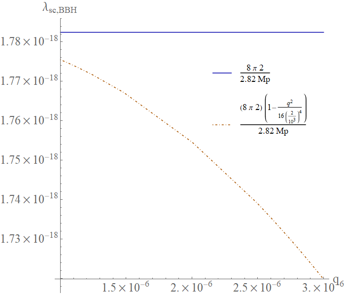
Figure 2: $\lambda_{\rm sc(BBH)}$ vs $q$ plot for $M_{p}\sim 10^{19}$ GeV

In Figure (1), we consider two values for $q$, such as $3.5\times 10^{-6}$ and $3\times 10^{-6}$, while we keep $\alpha=10^{-3}$. The chosen values for $q$ is restricted by the conditions $q<4\alpha^{2}\beta^{2}$ from Eq. (73) and a more stringent one appears from Eq. (10) as $q<\alpha^{2}\beta^{2}$. Therefore, throughout this analysis we choose the parameter space for $q$ such that it complies with the latter one. We list our analysis as below.

• For these choices of parameters $\lambda_{\rm sc\,(BBH)}$, both become $\mathcal{O}(10^{-19})\,{\rm GeV}^{-1}$. Evidently, the wavelengths corresponding to the emitted photon fields for both the black hole spacetimes are extremely small and far beyond the observational capacity.

• Although values for the $\lambda_{\rm sc\,(BBH)}$ is small, it is noteworthy that there are deviations in the values of $\lambda_{\rm sc}$ and $\lambda_{\rm BBH}$ with respect to the variation in $\beta$. The deviations are more evident for the smaller values of $\beta$. This suggests that for the black hole masses slightly greater or comparable to the Planck mass, the HBAR from the BBH and Schwarzschild black hole can be distinguished.

• For the larger value of $\beta$ the plots tentatively coincide with the standard Schwarzschild outcome. This dictates that for the BBHs with the masses larger than the Planck mass, the Schwarzschild potential $2M/M_{p}^{2}$ dominates over the tidal charge correction term in the metric of the BBH (see Eq. (8)) which eventually leads to the above outcome.

Subsequently, in Figure(2), we consider $\beta=2$ and $\alpha=10^{-3}$, while vary $q$ from $10^{-6}$ to $3\times 10^{-6}$. We list our analysis as below,

• Eqs. (10) and (73) dictate that $q$ cannot be increased arbitrarily. Thus obeying this constraint we obtain Figure (2) which showcase an attenuation in the wavelengths with the increasing values of $q$. A possible argument is that increase in the parameter $q$ implies an increment in the tidal effect, originating from the induced gravitational field on the brane. This increasing tidal effect leads to the squeezing of the wavelength of the emitted photons, which may alter the wavelengths of the emitted photons.

• For smaller value of $q$, the two curves corresponding to the standard Schwarzschild and BBH coincides. The Schwarzschild term will gradually become more dominating for decreasing tidal charge.

V Discussion

The phenomena of particle production in flat/ curved spacetime is consistently progressing since its proposition in the year 1973 [29, 30, 31, 32, 33, 34]. Plethora of novel outcomes, new techniques have been divulged in the studies of particle production and as well for its detection. In recent times, Scully etal.[1] have demonstrated that employing the quantum optical technique an alternative mechanism can be emanated which is based on the concept of virtual transition. This mechanism is designed using the model of cavity quantum electrodynamics and it reveals some distinctive features of the particle production due to the acceleration radiation in flat/ curved spacetime. In regard to the curved spacetime, for example the black hole spacetime we call this radiation process as HBAR. HBAR phenomena is well explored within the framework of GR, whereas its fate in the context of alternative theories of gravity have been rarely investigated. Thus, in this work we study the phenomena of HBAR in the background of a BBH spacetime which emerges as the lower dimensional effective theory on the visible brane from a five dimensional gravitational theory. We find the transition probability of the atoms and the HBAR entropy while allowing upto the quadratic power of the tidal charge. Our results depict that the transition probability depends on the quadratic power of the tidal charge and thus independent of the sign of the charge. However, its dependence on the tidal charge reflects the influence of bulk curvature effect in HBAR in the background of a higher dimensional theory. As mentioned in section (IV.1), we perform a comparative study between the behaviour of the wavelengths $\lambda_{\rm sc}$ and $\lambda_{\rm BBH}$ of the radiated photon fields, which corresponds to the maximum transition probability in the standard Schwarzschild and BBH spacetimes respectively. For this analysis, we follow the theory of Wien displacement. The values of $\lambda_{\rm sc\,(BBH)}$ come out to be extremely small [see Figures (1) and (2)] and currently far beyond the observational scope. However, Figure (1) dictates a theoretically alluring outcome that $\lambda_{\rm sc}$ and $\lambda_{\rm BBH}$ differ from each other for a certain mass range of the black hole, that is for, $M$ slightly greater or equal to $M_{p}$. We hope that a thorough investigation of this mass range of the black holes which can be categorised as the micro size black holes may shed some light upon the gravitational effects of the background spacetime and as well the acceleration radiation in such geometries. Figure (2) describes the decreasing pattern of the $\lambda_{\rm BBH}$ with increasing tidal charge of the black hole. This outcome also possesses theoretical merit such as this attenuating feature of the wavelength may arise due to the increasing tidal effect (as the tidal charge $q$ is increasing in the figure (2)) which emerges due to the projection of the bulk gravitational field on the $(3+1)$-dimensional visible brane. As a future direction, we hope to report soon the prominence of HBAR for other modified theories of gravity such as the higher curvature gravity theories.

Appendix A Some important equations

In this Appendix, we present some important equations used in the main text. We start by considering,

$$y=\,1+\,\frac{3\,x}{2\,\omega_{dl}}~{}.$$ (75)

Thus, we have (since $\frac{3x}{2\omega_{dl}}<1$)

$$y^{1/3}=\left(1+\frac{3x}{2\omega_{dl}}\right)^{1/3}\approx 1+\frac{x}{2\omega_{dl}}-\frac{x^{2}}{4\omega_{dl}^{2}}+\frac{5x^{3}}{24\omega_{dl}^{3}}$$

(76)

$$y^{-1/3}=\left(1+\frac{3x}{2\omega_{dl}}\right)^{-1/3}\approx 1-\frac{x}{2\omega_{dl}}+\frac{x^{2}}{2\omega_{dl}^{2}}-\frac{7x^{3}}{12\omega_{dl}^{3}}$$

(77)

$$y^{2/3}=\,\left(1+\,\frac{3\,x}{2\,\omega_{dl}}\right)^{2/3}\approx\,1+\frac{x}{\omega_{dl}}-\,\frac{x^{2}}{4\,\omega_{dl}^{2}}+\,\frac{x^{3}}{6\,\omega_{dl}^{3}}$$

(78)

$$P_{{\rm exc}}=\frac{4g^{2}_{dl}}{9}\Bigg{|}\bigintssss_{y=1}^{\infty}dyy^{-1/3}\Bigg{[}-y^{1/3}+\frac{Q_{dl}}{2}\left\{y^{1/3}-y^{-1/3}\right\}+\frac{3Q_{dl}^{2}}{8}\left\{2y^{-1/3}-y^{-1}-y^{-1/3}\right\}\Bigg{]}$$ (79)

$$\times {\rm exp}\bigg{[}-i\nu_{dl}\bigg{\{}y^{2/3}+2{\rm ln}\left(y^{1/3}-1\right)+2y^{1/3}+\frac{2y}{3}+2Q_{dl}{\rm ln}\left(y^{1/3}-1\right)-Q_{dl}+2Q_{dl}y^{1/3}-\frac{Q_{dl}y}{3}+2Q_{dl}^{2}{\rm ln}\left(1-y^{-1/3}\right)$$

$$- \frac{Q_{dl}^{2}}{2}-\frac{7Q_{dl}^{2}y^{1/3}}{4}+\frac{Q_{dl}^{2}y}{4}\bigg{\}}\bigg{]}{\rm exp}\bigg{[}i\omega_{dl}\bigg{\{}-\frac{2y}{3}+Q_{dl}\left(\frac{y}{3}-y^{1/3}\right)+Q_{dl}^{2}\left(\frac{3\,y^{1/3}}{2}+\frac{3\,y^{-1/3}}{4}-\frac{y}{4}\right)\bigg{\}}\bigg{]}\Bigg{|}^{2}$$

Appendix B Integration of eq.(40)

From Eq.(40), we write,

$$I=\,\bigintssss_{0}^{\infty}\,dx\,\left(1-A\,x+B\,x^{2}\right)\,(1+ip_{2}\,x^{2})\,x^{-2i\,\widetilde{\nu_{dl}}}\,e^{-ip_{1}\,x}$$

(80)

We take, $x=\frac{x^{\prime}}{p_{1}}$ which yields Eq (80) as below.

$$I = (p_{1})^{2i\widetilde{\nu_{dl}}-1}\bigintssss_{0}^{\infty}dx^{\prime}\left(1-\frac{Ax^{\prime}}{p_{1}}+\frac{Bx^{\prime 2}}{p_{1}^{2}}\right)$$ (81)

$$\times (x^{\prime})^{-2i\widetilde{\nu_{dl}}}e^{-ix^{\prime}}+ip_{2}(p_{1})^{2i\widetilde{\nu_{dl}}-3}\bigintssss_{0}^{\infty}dx^{\prime}\left(1-\frac{Ax^{\prime}}{p_{1}}+\frac{Bx^{\prime 2}}{p_{1}^{2}}\right)(x^{\prime})^{2-2i\widetilde{\nu_{dl}}}e^{-ix^{\prime}}~{}.$$

Integrating term by term we obtain, Let us take,

$$T_{1} =\,\int_{0}^{\infty}dx^{\prime}\,(x^{\prime})^{-2i\,\widetilde{\nu_{dl}}}\,e^{-i\,x^{\prime}}$$

$$=\,-\,2\,\widetilde{\nu_{dl}}\,e^{-\pi\,\widetilde{\nu_{dl}}}\,\,\Gamma[-\,2\,i\widetilde{\nu_{dl}}]$$ (82)

$$T_{2} =-\frac{A}{p_{1}}\int_{0}^{\infty}dx^{\prime}(x^{\prime})^{1-2i\widetilde{\nu_{dl}}}e^{-ix^{\prime}}$$

$$=-\frac{2iA}{p_{1}}\left\{\widetilde{\nu_{dl}}(1-2i\widetilde{\nu_{dl}})\right\}e^{-\pi\widetilde{\nu_{dl}}}\Gamma[-2i\widetilde{\nu_{dl}}]$$ (83)

$$T_{3} =\frac{B}{p_{1}^{2}}\int_{0}^{\infty}dx^{\prime}(x^{\prime})^{2-2i\widetilde{\nu_{dl}}}e^{-ix^{\prime}}$$

$$=\frac{4\,B}{p_{1}^{2}}\,\left\{\widetilde{\nu_{dl}}\,(1-i\,\widetilde{\nu_{dl}})\,(1-\,2i\,\widetilde{\nu_{dl}})\right\}\,e^{-\pi\,\widetilde{\nu_{dl}}}\,\,\Gamma[-\,2i\,\widetilde{\nu_{dl}}]$$ (84)

$$T_{4} =\int_{0}^{\infty}dx^{\prime}(x^{\prime})^{2-2i\widetilde{\nu_{dl}}}e^{-ix^{\prime}}$$

$$=4\,\left\{\widetilde{\nu_{dl}}\,(1-i\,\widetilde{\nu_{dl}})\,(1-\,2i\,\widetilde{\nu_{dl}})\right\}\,e^{-\pi\,\widetilde{\nu_{dl}}}\,\,\Gamma[-\,2\,i\widetilde{\nu_{dl}}]$$ (85)

$$T_{5} =-\frac{A}{p_{1}}\int_{0}^{\infty}dx^{\prime}(x^{\prime})^{3-2i\widetilde{\nu_{dl}}}e^{-ix^{\prime}}$$

$$=\frac{4iA}{p_{1}}\left\{\widetilde{\nu_{dl}}(1-i\widetilde{\nu_{dl}})(1-2i\widetilde{\nu_{dl}})(3-2i\widetilde{\nu_{dl}})\right\}$$

$$\times e^{-\pi\widetilde{\nu_{dl}}}\Gamma[-2i\widetilde{\nu_{dl}}]$$ (86)

$$T_{6} =\frac{B}{p_{1}^{2}}\int_{0}^{\infty}dx^{\prime}(x^{\prime})^{4-2i\widetilde{\nu_{dl}}}e^{-ix^{\prime}}$$

$$=-\frac{8B}{p_{1}^{2}}\bigg{\{}\widetilde{\nu_{dl}}(1-i\widetilde{\nu_{dl}})(1-2i\widetilde{\nu_{dl}})(2-i\widetilde{\nu_{dl}})$$

$$(3-2i\widetilde{\nu_{dl}})\bigg{\}}e^{-\pi\widetilde{\nu_{dl}}}\Gamma[-2i\widetilde{\nu_{dl}}]$$ (87)

Using $\frac{\nu_{dl}}{\omega_{dl}}\ll\,1$ and allowing all expansions upto the $\mathcal{O}(Q_{dl}^{2})$, one obtains $\frac{A}{p_{1}}\,\sim\,A$ and $\frac{B}{p_{1}^{2}}\,\sim\,B$. Thus we get,

$$T_{1} + T_{2}+T_{3}=\Bigg{[}-\frac{i\nu_{dl}}{\omega_{dl}}Q_{dl}(1+Q_{dl})-2\nu_{dl}\bigg{\{}1+Q_{dl}$$

$$\left(1+\frac{\nu_{dl}}{\omega_{dl}}\right)+Q_{dl}^{2}\left(1+\frac{2\nu_{dl}}{\omega_{dl}}\right)\bigg{\}}\Bigg{]}e^{-\pi\widetilde{\nu_{dl}}}\Gamma[-2i\widetilde{\nu_{dl}}]$$

$$T_{4} +T_{5}+T_{6}=\bigg{[}4\nu_{dl}\bigg{\{}1+Q_{dl}\left(1+\frac{11\nu_{dl}}{2\omega_{dl}}\right)$$ (89)

$$+Q^{2}_{dl}\left(1+\frac{11\nu_{dl}}{\omega_{dl}}\right)\bigg{\}}-8\nu_{dl}^{3}\bigg{\{}1+3Q_{dl}\left(1+\frac{\nu_{dl}}{3\,\omega_{dl}}\right)$$

$$+6Q_{dl}^{2}\left(1+\frac{2\nu_{dl}}{3\omega_{dl}}\right)\bigg{\}}+\frac{6\,i\nu_{dl}}{\omega_{dl}}\,Q_{dl}\left(1+Q_{dl}\right)$$

$$-12\,i\,\nu_{dl}^{2}\left\{1+2Q_{dl}\left(1+\frac{\nu_{dl}}{\omega_{dl}}\right)+3Q_{dl}^{2}\left(1+\frac{2\nu_{dl}}{\omega_{dl}}\right)\right\}\bigg{]}$$

$$e^{-\pi\,\widetilde{\nu_{dl}}}\,\,\Gamma[-\,2i\,\widetilde{\nu_{dl}}]$$

Eq (81) yields,

$$|\,I\,|^{2} = \frac{1}{p_{1}^{2}}\Bigg{|}\bigg{\{}-2\nu_{dl}+Q_{dl}\nu_{dl}\left(\frac{\nu_{dl}}{\omega_{dl}}-2\right)(1+2Q_{dl})\bigg{\}}$$ (90)

$$-i\Bigg{\{}\frac{2\nu_{dl}^{3}}{\omega_{dl}}Q_{dl}(1+3Q_{dl})\Bigg{\}}\Bigg{|}^{2}e^{-2\pi\widetilde{\nu_{dl}}}\Big{|}\Gamma[-2i\widetilde{\nu_{dl}}]\Big{|}^{2}$$

$$= \frac{1}{p_{1}^{2}}\Big{|}G-iH\Big{|}^{2}e^{-2\pi\widetilde{\nu_{dl}}}\Big{|}\Gamma[-2i\widetilde{\nu_{dl}}]\Big{|}^{2}]$$

$$= \frac{1}{p_{1}^{2}}(G^{2}+H^{2})e^{-2\pi\widetilde{\nu_{dl}}}\Big{|}\Gamma[-2i\widetilde{\nu_{dl}}]\Big{|}^{2}$$

$$= \frac{4\nu_{dl}^{2}}{p_{1}^{2}}\bigg{[}1+2Q_{dl}\left(1-\frac{\nu_{dl}}{2\omega_{dl}}\right)+5Q_{dl}^{2}\left(1-\frac{3\nu_{dl}}{2\omega_{dl}}\right)\bigg{]}$$

$$e^{-2\pi\widetilde{\nu_{dl}}}\Big{|}\Gamma[-2i\widetilde{\nu_{dl}}]\Big{|}^{2}~{}.$$

In the above equation, $G=-2\nu_{dl}+Q_{dl}\nu_{dl}\left(\frac{\nu_{dl}}{\omega_{dl}}-2\right)(1+2\,Q_{dl})$ and $H=\frac{2\,\nu_{dl}^{3}}{\omega_{dl}}\,Q_{dl}(1+3\,Q_{dl})$. We also use, $\Big{|}\Gamma[-i\,z]\Big{|}^{2}=\,\frac{\pi}{z\,{\rm Sinh}(\pi\,z)}$ in the above equation where $z=2\,\widetilde{\nu_{dl}}$. Thus we obtain,

$$|\,I\,|^{2} = \frac{4\pi\nu_{dl}^{2}}{p_{1}^{2}\widetilde{\nu_{dl}}}\bigg{[}1+2Q_{dl}\left(1-\frac{\nu_{dl}}{2\omega_{dl}}\right)+5Q_{dl}^{2}\left(1-\frac{3\nu_{dl}}{2\omega_{dl}}\right)\bigg{]}$$ (91)

$$\frac{1}{e^{4\pi\widetilde{\nu_{dl}}}-1}$$

In Eq. (91), we explicitly use the form of $p_{1}$ from Eq. (39c) and obtain the transition probability as,

$$P_{exc} = \frac{4\pi g^{2}_{dl}\nu_{dl}}{\omega_{dl}^{2}\left(1+\frac{2\nu_{dl}}{\omega_{dl}}\right)^{2}}\bigg{[}1+2Q_{dl}\left(1-\frac{\nu_{dl}}{2\omega_{dl}}\right)+5Q_{dl}^{2}\times$$ (92)

$$\left(1-\frac{3\nu_{dl}}{2\omega_{dl}}\right)\bigg{]}\left(1+Q_{dl}+Q^{2}_{dl}\right)^{-1}\bigg{[}1-\frac{Q_{dl}\nu_{dl}}{2\omega_{dl}}(1$$

$$+ 5Q_{dl})\left(1+\frac{2\nu_{dl}}{\omega_{dl}}\right)^{-1}\bigg{]}^{-2}\,\frac{1}{e^{4\pi\,\widetilde{\nu_{dl}}}-1}~{}.$$

We further approximate the above equation while allowing upto the linear order of $\frac{\nu_{dl}}{\omega_{dl}}$ and quadratic order of $Q_{dl}$. This yields,

$$P_{exc} = \frac{4\,\pi g^{2}_{dl}\,\nu_{dl}}{\omega_{dl}^{2}\left(1+\frac{2\nu_{dl}}{\omega_{dl}}\right)^{2}}\bigg{[}1+Q_{dl}+3\,Q_{dl}^{2}\left(1+\frac{4\,\nu_{dl}}{3\,\omega_{dl}}\right)\bigg{]}$$ (93)

$$\times \frac{1}{e^{4\pi\,\widetilde{\nu_{dl}}}-1}~{}.$$