INTERACTING URN MODELS WITH STRONG REINFORCEMENT

Abstract.

We disprove a conjecture by Launay [16] that almost surely one color monopolizes all the urns for the interacting urn model with polynomial reinforcement and parameter $p>0$. Moreover, we prove that the critical parameter $p_{m}$ converges to $1/2$ as $m$, the degree of the polynomial, goes to infinity.

In the case $p=1$, Launay [17] proved that a.s. one color monopolizes all the urns if the reinforcement sequence is non-decreasing and reciprocally summable. We give a short proof of that result and generalize it to a larger class of reinforcement sequences.

1. General introduction

1.1. Definitions and main results

The Pólya urn model and its variants are basic models of random processes with reinforcement. Recently, there is a growing interest in the study of systems of interacting urns, see e.g. [1] [4] [7] [8] [10] [13] [14] [19] [21]. In this paper, we study a model of (strongly) reinforced interacting urns introduced by Launay [16].

The aim of this paper is to disprove a conjecture by Launay [16] on this model and generalize the results in [17].

Let $\{W(n)\}_{n\in\mathbb{N}}$ be a positive sequence ($W(0)=0$ is allowed). Given $d$ urns of black and red balls, labeled by $u_{1},u_{2},\cdots,u_{d}$, we let $\eta:=\{\eta_{n}^{(1)}\}_{1\leq i\leq d,n\geq 1}$ be i.i.d. Bernoulli(p) random variables where $p\in[0,1]$. For $i\in\{1,2,\cdots,d\}$, we denote by $B_{n}(i)$ and $R_{n}(i)$, respectively, the number of black and red balls in the urn $u_{i}$ at time step $n$. Then, $B_{n}^{*}:=\sum_{i=1}^{d}B_{n}(i)$, resp. $R_{n}^{*}:=\sum_{i=1}^{d}R_{n}(i)$, is the total number of black balls, resp. red balls, in the system at time step $n$. At time 0, the initial composition is given by $(B_{0},R_{0})\in\mathbb{N}^{2d}$. For $n\in\mathbb{N}$, at time $n+1$, for $i\in\{1,2,\cdots,d\}$, we define a Bernoulli random variable $\xi_{n+1}(i)$ by

(1) $$\mathbb{P}(\xi_{n+1}(i)=1|\mathcal{G}_{n},\eta)=\frac{\mathds{1}_{\{\eta_{n+1}^{(i)}=1\}}W(B_{n}^{*})}{W(B_{n}^{*})+W(R_{n}^{*})}+\frac{\mathds{1}_{\{\eta_{n+1}^{(i)}=0\}}W(B_{n}(i))}{W(B_{n}(i))+W(R_{n}(i))}$$

where $\mathcal{G}_{n}:=\sigma(B_{m},R_{m}:m\leq n)$ with $B_{m}:=(B_{m}(i))_{1\leq i\leq d}$ and $R_{m}:=(R_{m}(i))_{1\leq i\leq d}$. Now set

(2) $$B_{n+1}(i):=B_{n}(i)+\xi_{n+1}(i),\quad R_{n+1}(i):=R_{n}(i)+1-\xi_{n+1}(i)$$

In particular, for any $i\in\{1,2,\cdots,d\}$ and $n\in\mathbb{N}$

(3) $$B_{n}(i)+R_{n}(i)=B_{0}(i)+R_{0}(i)+n,\quad B^{*}_{n}+R_{n}^{*}=dn+B_{0}^{*}+R_{0}^{*}$$

This process $(B_{n},R_{n})_{n\in\mathbb{N}}$ is called the interacting urn mechanism (IUM) with reinforcement sequence $\{W(n)\}_{n\in\mathbb{N}}$ and interaction parameter $p$. We denote its law by $\mathbb{P}_{p}^{W}$.

Remark 1.1.

In words, we draw at each step and for each urn a red or black ball from either all the urns combined (with probability $p$) or the urn alone (with probability $1-p)$ and add a new ball of the same color to this urn. The probability of drawing a ball of a certain color is proportional to $W(k)$ where $k$ is the number of balls of this color. The case $d=1$ is an ordinal-dependent version of Pólya’s urn, see e.g. Section 3.2 [20] or Appendix [11].

Unless otherwise specified, we assume $d=2$ (i.e. two urns) for simplicity. Note that many results in this paper can be generalized to the cases $d\geq 2$. Let

(4) $$x_{n}:=\frac{B_{n}(1)}{n+B_{0}(1)+R_{0}(1)},\quad y_{n}:=\frac{B_{n}(2)}{n+B_{0}(2)+R_{0}(2)}$$

be the proportion of black balls in $u_{1}$ and $u_{2}$, respectively, at time step $n$.

For an IUM with $p>0$, there is a tendency for different components to adopt a common behavior. For example, for IUM with linear reinforcements, e.g. $W(n)=n$, in [10], it has been shown that the urns synchronize a.s. as long as $p>0$, i.e.

$$\lim_{n\to\infty}x_{n}=\lim_{n\to\infty}y_{n}\quad\text{exists}\quad a.s.$$

but $\mathbb{P}(\lim_{n\to\infty}(x_{n},y_{n})\in\{(0,0),(1,1)\})<1$. However, IUM with strong reinforcement may exhibit very different behaviors.

Assumption 1.1 (Strong reinforcement).

Throughout this paper, we focus on strong reinforcement sequences, i.e. $\{W(n)\}_{n\in\mathbb{N}}$ satisfies

(5) $$\sum_{n=1}^{\infty}\frac{1}{W(n)}<\infty$$

As we will see later, for some IUMs with weak interaction (i.e. $p$ is small), the reinforcement is strong enough so that one color can maintain its advantage in a single urn while it is at a disadvantage globally, in which case the urns do not synchronize. On the other hand, for strong interaction, the phenomena of domination and monopoly may occur.

Definition 1 (Domination and monopoly).

We denote by

$$\mathcal{D}=\left\{\lim_{n\rightarrow\infty}(x_{n},y_{n})=(0,0)\right\}\cup\left\{\lim_{n\rightarrow\infty}(x_{n},y_{n})=(1,1)\right\}$$

the event that eventually the number of balls of one color is negligible with respect to the number of balls of the other color, and call this event domination. Further, we denote by

$$\mathcal{M}=\left\{R^{*}_{n+1}=R^{*}_{n}\text{ eventually for all }n\right\}\cup\left\{B^{*}_{n+1}=B^{*}_{n}\text{ eventually for all }n\right\}$$

the event that eventually only balls of one color are added to the urns, and call this event monopoly.

Remark 1.2.

Immediately, we have $\mathcal{M}\subset\mathcal{D}$, and thus $\mathbb{P}(\mathcal{M})\leq\mathbb{P}(\mathcal{D})$.

Launay [16] proved that IUM with exponential reinforcement exhibits a phase transition at $p=1/2$.

Theorem 1.1 (Theorem 3.2 [16]).

Assume $W(n)=\rho^{n},n\in\mathbb{N}$, for some $\rho>1$. If $p\geq 1/2$, then $\mathbb{P}_{p}^{W}(\mathcal{M})=1$. If $p<1/2$, then with positive probability, there exists a finite (random) time $n_{0}$ such that

(6) $$\xi_{n}(1)=\eta_{k+1}^{(1)},\quad\xi_{n}(2)=1,\quad\forall n>n_{0}$$

That is, at any time $n>n_{0}$, black balls are added to the first urn if and only if $\eta_{n}^{(1)}=1$ (i.e. all the urns combined), and only black balls are added to the second urn.

Remark 1.3.

As $\rho$ tends to $\infty$, this reinforcement mechanism converges to the “generalized” reinforcement, which was introduced and studied by Launay and Limic in [18].

1.1.1. Polynomial reinforcement

Launay conjectured that for polynomial reinforcement, $\mathbb{P}_{p}^{W}(\mathcal{M})=1$ for any $p>0$.

Definition 2 (Polynomial reinforcement).

For any $m\geq 2$, let $(B_{n},R_{n})_{n\in\mathbb{N}}$ is an IUM with $(B^{*}_{0},R_{0}^{*})\in\mathbb{N}^{+}\times\mathbb{N}^{+}$ and parameter $p\in[0,1]$. The reinforcement sequence is given by

(7) $$W(n):=a_{m}n^{m}+a_{m-1}n^{m-1}+\cdots+a_{0},\quad n\in\mathbb{N}$$

where $a_{m}>0,a_{0},a_{1},\cdots,a_{m-1}\geq 0$. We denote its law by $\mathbb{P}_{p}^{(m)}$. We define the critical parameter

(8) $$p_{m}=\inf\{0\leq q\leq 1:\mathbb{P}_{p}^{(m)}(\mathcal{D})=1,\ \forall p\geq q\}$$

Remark 1.4.

(i) As we will see later, the asymptotic behavior of $(x_{n},y_{n})$ depends only on $m$ and $p$ but not on $a_{m},a_{m-1},\cdots,a_{0}$. This is why we use the notation $\mathbb{P}_{p}^{(m)}$.
(ii) Note that $\mathbb{P}^{(m)}_{1}(\mathcal{D})=1$ by Theorem 2.3 [17]. Thus, the set in the right-hand side of (8) is non-empty.

The following theorem implies that $\mathbb{P}_{p}^{(m)}(\mathcal{M})\leq\mathbb{P}_{p}^{(m)}(\mathcal{D})<1$ for small $p$, which disproves Launay’s conjecture.

Theorem 1.2.

Let $m\geq 2$, for any $p\in[0,1]$, $\mathbb{P}_{p}^{(m)}((x_{n},y_{n})\ \text{converges})=1$ . Moreover, there exists $q_{m}>0$ such that if $p<q_{m}$, then

$$\mathbb{P}_{p}^{(m)}(\lim_{n\to\infty}(x_{n},y_{n})=(u_{m},1-u_{m}))>0$$

and thus $\mathbb{P}_{p}^{(m)}(\mathcal{D})<1$, where $u_{m}$ is the unique solution of the equation

$$u=\frac{(1-p)u^{m}}{u^{m}+(1-u)^{m}}+\frac{p}{2}$$

on $[0,1/2)$. In particular, $p_{m}\geq q_{m}>0$.

For $m=2$, we give a lower bound for the critical parameter $p_{2}$.

Proposition 1.3.

If $p<1-\sqrt{2}/2$, then

$$\mathbb{P}^{(2)}_{p}(\lim_{n\to\infty}(x_{n},y_{n})=(\frac{1-\sqrt{1-2p}}{2},\frac{1+\sqrt{1-2p}}{2}))>0$$

In particular, the critical parameter $p_{2}\geq 1-\sqrt{2}/2$.

For exponential reinforcement, the critical parameter is $1/2$ by Theorem 1.1. Moreover, by the law of large numbers, a.s. on the event that (6) occurs, $(x_{n},y_{n})$ converges to $(p,1)$. We show that polynomial reinforcement is weaker than exponential reinforcement in the sense that $p_{m}<1/2$. On the other hand, for large $m$, we expect that the polynomial reinforcement is very strong in the sense that $\lim_{m\to\infty}p_{m}=1/2$, and with positive probability, $\lim_{n\to\infty}(x_{n},y_{n})$ is in a small neighborhood of $(p,1)$. The following theorem validates this statement.

Theorem 1.4.

For any $m\geq 2$, $p_{m}<1/2$. Moreover, $\lim_{m\to\infty}p_{m}=1/2$. More precisely, given $p<1/2$, for large $m$, there exists $s_{m}\in(0,1)\times(0,1)$ such that

$$\mathbb{P}_{p}^{(m)}(\lim_{n\to\infty}(x_{n},y_{n})=s_{m})>0,\quad\lim_{m\to\infty}s_{m}=(p,1)$$

For polynomial reinforcement, almost surely, domination implies monopoly.

Proposition 1.5.

$\mathbb{P}_{p}^{(m)}(\mathcal{D}\backslash\mathcal{M})=0$. In particular, $\mathbb{P}_{p}^{(m)}(\mathcal{M})=1$ if $p>p_{m}$.

1.1.2. Urns with simultaneous drawing

The case $p=1$ was studied in [17]. The main result of [17] is the following where $d\geq 2$ is arbitrary.

Theorem 1.6 (Theorem 2.3 [17]).

For $d\geq 2$, assume that $\{W(n)\}_{n\in\mathbb{N}}$ is non-decreasing and satisfies (5), then $\mathbb{P}_{1}^{W}(\mathcal{M})=1$.

Remark 1.5.

The case $d=1$ was proved by Davis [11] where the assumption that $W$ is non-decreasing is not needed. An elegant proof using a continuous time construction of urn processes can be found in [11] or [20]

We prove a stronger result and will not limit ourselves to two-color urns. In this case, it is convenient to assume that we have only a single urn of $N_{c}$ $(N_{c}\geq 2)$ colors. Let $N_{n}(i)$ be the number of balls of the $i$-th color in this urn at time step $n$, and write $N_{n}:=(N_{n}(i))_{1\leq i\leq N_{c}}$. Let $\mathcal{G}_{n}:=\sigma(N_{m}:m\leq n)$. At time 0, assume $N_{0}(i)=a_{i}\in\mathbb{N}^{+}$ ($i=1,2,\cdots,N_{c}$). At time $n+1$, conditional on $\mathcal{G}_{n}$, the law of $(N_{n+1}(i)-N_{n}(i))_{1\leq i\leq N_{c}}$ follows a multinomial distribution $M(d;W(N_{n}(i))/\sum_{j=1}^{N_{c}}W(N_{j}(n)),1\leq i\leq N_{c})$. Note that the case $N_{c}=2$ is the model studied in [17]. For $N_{c}\geq 2$, we define the event monopoly by

$$\mathcal{M}=\left\{\exists i\in\{1,2,\cdots,N_{c}\},\ s.t.\ N_{n+1}(j)=N_{n}(j)\text{ for all large n and }\ j\neq i\right\}$$

Theorem 1.7.

Assume that (5) holds and there exists a positive constant $C$ such that

(9) $$W(n)\sum_{k=n}^{\infty}|\frac{1}{W(k)}-\frac{1}{W(k+1)}|\leq C,\quad\forall n\geq 1$$

Then, $\mathbb{P}_{1}^{W}(\mathcal{M})=1$.

Remark 1.6.

If $\{W(n)\}$ is non-decreasing and satisfies (5), then (9) holds with $C=1$. Thus, Theorem 1.7 implies Theorem 1.6.

A direct consequence of Theorem 1.7 is the following.

Corollary 1.8.

Assume that (5) holds and there exists a positive constant $C$ such that

(10) $$W(n)\sum_{k=n}^{\infty}\frac{1}{W(k)}\leq C,\quad\forall n\geq 1$$

Then, $\mathbb{P}_{1}^{W}(\mathcal{M})=1$.

Example 1.1.

(i) Let $\{W(n)\}_{n\in\mathbb{N}}$ be such that

$$W(2n)=n^{4},\quad W(2n+1)=n^{4}-n^{3}+1,\quad n\in\mathbb{N}$$

Then (5) and (9) are satisfied but $W$ is not an increasing function. By Theorem 1.7, one color monopolizes a.s..
(ii) Let $\{W(n)\}_{n\in\mathbb{N}}$ be such that

$$W(2n)=e^{n},\quad W(2n+1)=e^{n-1},\quad n\in\mathbb{N}$$

Then (5) and (10) are satisfied but $W$ is not an increasing function. Indeed,

$$\frac{W(2n+1)}{W(2n)}=\frac{1}{e},\quad\quad n\in\mathbb{N}$$

By Corollary 1.8, one color monopolizes a.s..

1.2. Introduction to the proofs and the techniques

1.2.1. Stochastic approximation algorithms

The type of stochastic approximation process we will be interested in is a Robbins-Monro algorithm. For an introduction to stochastic approximation algorithms, see e.g. [3] [5] [6] [12].

Let $\{W(n)\}_{n\in\mathbb{N}}$ be a polynomial reinforcement sequence as in (7). We show that the random process defined by (4) is generated by a stochastic approximation algorithm.

Proposition 1.9.

Under $\mathbb{P}_{p}^{(m)}$, $\{(x_{n},y_{n})\}_{n\in\mathbb{N}}$ defined in (4) satisfies the following recursion:

(11) $$(x_{n+1},y_{n+1})-(x_{n},y_{n})=\frac{1}{n+1}(F^{(m)}(x_{n},y_{n})+\varepsilon_{n+1}+\eta_{n+1}),\quad n\in\mathbb{N}$$

where $F^{(m)}=(F_{1}^{(m)},F_{2}^{(m)})$ is a vector function on $[0,1]^{2}$ defined by

$$F_{1}^{(m)}(x,y)=-x+\frac{(1-p)x^{m}}{x^{m}+(1-x)^{m}}+\frac{p(x+y)^{m}}{(x+y)^{m}+(2-x-y)^{m}}$$

$$F_{2}^{(m)}(x,y)=-y+\frac{(1-p)y^{m}}{y^{m}+(1-y)^{m}}+\frac{p(x+y)^{m}}{(x+y)^{m}+(2-x-y)^{m}}$$

$\{\varepsilon_{n+1}\}_{n\in\mathbb{N}}=\{(\varepsilon_{n}(1),\varepsilon_{n}(2))\}_{n\in\mathbb{N}}$ is a bounded martigale difference sequence, and $\{\eta_{n+1}\}_{n\in\mathbb{N}}=\{(\eta_{n+1}(1),\eta_{n+1}(2))\}_{n\in\mathbb{N}}$ satisfies

$$\|\eta_{n}\|\leq\frac{C}{n+1},\quad\forall n\in\mathbb{N}$$

for some positive constant $C$.

Proof.

By (1), for any $n\in\mathbb{N}$,

$$\mathbb{E}(\xi_{n+1}(1)|\mathcal{G}_{n})=(1-p)\frac{W(B_{n}(i))}{W(B_{n}(1))+W(R_{n}(1))}+p\frac{W(B_{n}^{*})}{W(B_{n}^{*})+W(R_{n}^{*})}$$

Divide the numerator and denominator by $a_{m}(n+1)^{m}$ and use (3),

$$\mathbb{E}(\xi_{n+1}(1)|\mathcal{G}_{n}) =(1-p)\frac{x_{n}^{m}+O(\frac{1}{n})}{x_{n}^{m}+(1-x_{n})^{m}+O(\frac{1}{n})}+p\frac{(x_{n}+y_{n})^{m}+O(\frac{1}{n})}{(x_{n}+y_{n})^{m}+(2-x-y)^{m}+O(\frac{1}{n})}$$

$$=\frac{(1-p)x_{n}^{m}}{x_{n}^{m}+(1-x_{n})^{m}}+\frac{p(x_{n}+y_{n})^{m}}{(x_{n}+y_{n})^{m}+(2-x_{n}-y_{n})^{m}}+O(\frac{1}{n})$$

By (2), we have

$$x_{n+1}-x_{n} =\frac{B_{n+1}(1)-B_{n}(1)-x_{n}}{n+1+B_{0}(1)+R_{0}(1)}=\frac{-x_{n}+\mathbb{E}(\xi_{n+1}(1)|\mathcal{G}_{n})}{n+1+B_{0}(1)+R_{0}(1)}+\frac{\xi_{n+1}(1)-\mathbb{E}(\xi_{n+1}(1)|\mathcal{G}_{n})}{n+1+B_{0}(1)+R_{0}(1)}$$

$$=\frac{1}{n+1}(F_{1}^{(m)}(x_{n},y_{n})+\varepsilon_{n+1}(1)+\eta_{n+1}(1))$$

where

(12) $$\varepsilon_{n+1}(1):=\frac{n+1}{n+1+B_{0}(1)+R_{0}(1)}\left(\xi_{n+1}(1)-\mathbb{E}(\xi_{n+1}(1)|\mathcal{G}_{n})\right)$$

and

$$\eta_{n+1}(1):=(n+1)\frac{-x_{n}+\mathbb{E}(\xi_{n+1}(1)|\mathcal{G}_{n})}{n+1+B_{0}(1)+R_{0}(1)}-F_{1}^{(m)}(x_{n},y_{n})=O(\frac{1}{n})$$

The equation for $y_{n+1}-y_{n}$ is proved similarly. ∎

Remark 1.7.

Our approach applies to more general cases where the conditional probability of drawing a color depends only on the relative frequency. In the case of polynomial reinforcement, asymptotically (up to a small error term), the conditional probability of drawing a black ball depends only on $F^{(m)}(x_{n},y_{n})$.

We are interested in the planar linear system $(dx/dt,dy/dt)=F^{(m)}(x,y)$, i.e.

(13) $$\left\{\begin{aligned} \frac{dx}{dt}&=-x+\frac{(1-p)x^{m}}{x^{m}+(1-x)^{m}}+\frac{p(x+y)^{m}}{(x+y)^{m}+(2-x-y)^{m}}\\ \frac{dy}{dt}&=-y+\frac{(1-p)y^{m}}{y^{m}+(1-y)^{m}}+\frac{p(x+y)^{m}}{(x+y)^{m}+(2-x-y)^{m}}\end{aligned}\right.$$

with initial condition $(x(0),y(0))\in[0,1]^{2}$. Note that if $(x(t),y(t))$ is a solution to (13) with $(x(0),y(0))\in[0,1]^{2}$, then $(x(t),y(t))\in[0,1]^{2}$ for all $t\in[0,\infty)$.

Definition 3 (Equilibrium point).

A point $(x,y)\in[0,1]^{2}$ is called an equilibrium of (13) if $F^{(m)}(x,y)=0$. It is said to be a stable (resp. strictly stable) equilibrium if all the eigenvalues of $DF^{(m)}(x,y)$ have nonpositive (resp. negative) eigenvalues, and it is called unstable if one of the eigenvalues of $DF^{(m)}(x,y)$ has positive real part. Let $\Lambda^{(m)}$ be the set of all equilibrium points, and let $\mathcal{E}_{s}^{(m)}$ be the set of strictly stable equilibria of (13).

Note that

$$DF^{(m)}(x,y)=\left(\begin{array}[]{ll}-1+m(1-p)f(x)+\frac{mp}{2}f(\frac{x+y}{2})&\frac{mp}{2}f(\frac{x+y}{2})\\ \frac{mp}{2}f(\frac{x+y}{2})&-1+m(1-p)f(y)+\frac{mp}{2}f(\frac{x+y}{2})\end{array}\right)$$

where $f$ is defined by

(14) $$f(t):=\frac{t^{m-1}(1-t)^{m-1}}{[t^{m}+(1-t)^{m}]^{2}},\quad t\in[0,1]$$

$DF^{(m)}(x,y)$ is a real symmetric matrix and thus has two real eigenvalues:

(15) $$\lambda_{\pm}(x,y) =-1+\frac{mp}{2}f(\frac{x+y}{2})+m(1-p)\frac{f(x)+f(y)}{2}$$

$$\pm\frac{1}{2}\sqrt{m^{2}(1-p)^{2}(f(x)-f(y))^{2}+m^{2}p^{2}f^{2}(\frac{x+y}{2})}$$

Therefore, for $(x,y)\in\Lambda^{(m)}$,

$$(x,y)\in\mathcal{E}_{s}^{(m)}\Leftrightarrow\lambda_{+}(x,y)<0,\quad(x,y)\ \text{is stable (resp. unstable)}\Leftrightarrow\lambda_{+}(x,y)\leq 0\ (\text{resp.}>0)$$

Example 1.2.

$(1/2,1/2)\in\Lambda^{(m)}$ is unstable since $\lambda_{+}(\frac{1}{2},\frac{1}{2})=m-1>0$. $(0,0)$ and $(1,1)$ are strictly stable equilibria since $\lambda_{+}(0,0)=\lambda_{+}(1,1)=-1$.

For the equilibria set, we prove the following result.

Proposition 1.10.

$\Lambda^{(m)}$ is a finite set including $(0,0),(1/2,1/2),(1,1)$. Moreover, if $p=0$,

$$\Lambda^{(m)}=\{0,\frac{1}{2},1\}\times\{0,\frac{1}{2},1\}$$

If $p>0$, then

$$\Lambda^{(m)}\backslash\{(0,0),(\frac{1}{2},\frac{1}{2}),(1,1)\}\subset\left((0,\frac{1}{2})\times(\frac{1}{2},1)\right)\cup\left((\frac{1}{2},1)\times(0,\frac{1}{2})\right)$$

For the cases $m=3,p=0.4$ and $m=5,p=0.3$, $\Lambda^{(m)}$ are plotted in Figure 1 ($\Lambda^{(m)}$ is the set of intersection points of the two curves).

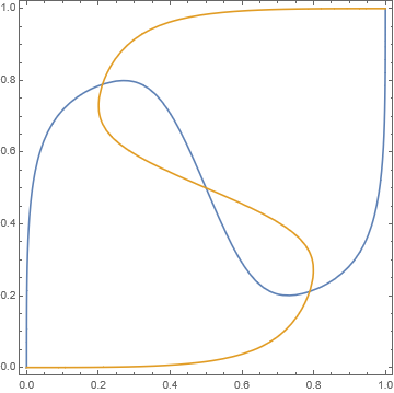
(a) m=3, p=0.4

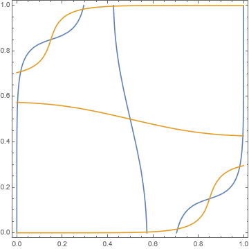
(b) m=5, p=0.3

Figure 1. $F_{1}^{(m)}(x,y)=0$ in blue and $F_{2}^{(m)}(x,y)=0$ in orange

It turns out that the system (13) is a gradient system. We define $L^{(m)}:[0,1]^{2}\to\mathbb{R}$ by

(16) $$L^{(m)}(x,y)=(1-p)G^{(m)}(x)+(1-p)G^{(m)}(y)+2pG^{(m)}(\frac{x+y}{2})$$

where

$$G^{(m)}(t):=\int_{0}^{t}\frac{u^{m}}{u^{m}+(1-u)^{m}}du,\quad t\in[0,1]$$

Example 1.3.

For $m=2,3$, we have

$$L^{(2)}(x,y) =\frac{1-p}{4}\log(x^{2}+(1-x)^{2})+\frac{1-p}{4}\log(y^{2}+(1-y)^{2})$$

$$+\frac{p}{2}\log((x+y)^{2}+(2-x-y)^{2})-p\log 2-\frac{x^{2}}{2}+\frac{x}{2}-\frac{y^{2}}{2}+\frac{y}{2}$$

and

$$L^{(3)}(x,y) =\frac{1-p}{9}\left(\log(x^{3}+(1-x)^{3})+\log(y^{3}+(1-y)^{3})\right)+\frac{2p}{9}\log((x+y)^{3}+(2-x-y)^{3})$$

$$-\frac{2p}{3}\log 2-\frac{4+p}{12}x^{2}-\frac{4+p}{12}y^{2}+\frac{pxy}{6}+\frac{x+y}{3}$$

The proof of the following result is direct and is omitted here.

Proposition 1.11.

For any $m\geq 2$, let $L^{(m)}$ be as in (16). We have

$$\operatorname{grad}L^{(m)}=F^{(m)}$$

In particular, $L^{(m)}$ is a strict Lyapunov function for $F^{(m)}$, i.e. $L^{(m)}$ is strictly monotone along any integral curve of $F^{(m)}$ outside $\Lambda^{(m)}$

Thus, the stochastic approximation algorithm (11) is a stochastic gradient scheme. By results from stochastic approximation theory, we have the following result which implies the first assertion in Theorem 1.2.

Proposition 1.12.

Let $m\geq 2$ and $p\in[0,1]$, almost surely for $\mathbb{P}_{p}^{(m)}$, $\lim_{n\to\infty}(x_{n},y_{n})$ exists and belongs to $\Lambda^{(m)}$.

Proof.

This is a direct result of Corollary 6.6 [3] and Proposition 1.10. ∎

Definition 4 (Attractor).

Let $\{\Phi_{t}\}_{t\in\mathbb{R}}$ be the flow generated by (13). A subset $A\subset[0,1]^{2}$ is an attractor for $\{\Phi_{t}\}_{t\in\mathbb{R}}$ provided:
(i) $A$ is nonempty, compact and invariant (i.e. $\Phi_{t}A=A,\ \forall t\in\mathbb{R})$; and
(ii) $A$ has a neighborhood $U\subset[0,1]^{2}$ such that $\operatorname{dist}\left(\Phi_{t}x,A\right)\rightarrow 0$ as $t\rightarrow\infty$ uniformly in $x\in U$.

By ODE theory, see e.g. Theorem 3.13 [2] or Theorem 9.4 [24], $(x,y)$ is an attractor if $(x,y)\in\mathcal{E}_{s}^{(m)}$. Then, by Theorem 7.3 [3], we have the following result.

Proposition 1.13.

For any $(x,y)\in\mathcal{E}_{s}^{(m)}$, we have

$$\mathbb{P}_{p}^{(m)}(\lim_{n\to\infty}(x_{n},y_{n})=(x,y))>0$$

By Proposition 1.13, to prove Theorem 1.2, it suffices to show that if $p$ is small, then $(u_{m},1-u_{m})\in\mathcal{E}_{s}^{(m)}$. For the cases $m=3,p=0.2$ and $m=4,p=0.15$, the vector fields generated by (13) are plotted in Figure 2. Readers can find strictly stable equilibria $(u_{m},1-u_{m})$, $m=3,4$, inside the red circles.

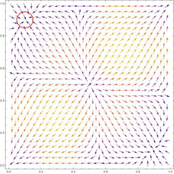
(a) m=3, p=0.2

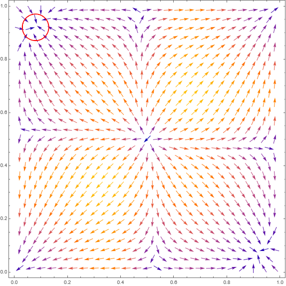
(b) m=4, p=0.15

Figure 2. The vector fields generated by (13) for small p

On the other hand, for unstable equilibria, we prove the following result.

Proposition 1.14.

If $(x,y)\in\Lambda^{(m)}$ is unstable, then

(17) $$\mathbb{P}_{p}^{(m)}(\lim_{n\to\infty}(x_{n},y_{n})=(x,y))=0$$

Proof.

Since $(x,y)$ is unstable, it is not on the boundary of $[0,1]^{2}$, and thus there exists a neighborhood $\mathcal{N}$ of $(x,y)$ such that any $(u,v)\in\mathcal{N}$ is bounded away from the boundary. Now we show that there exists a constant $b>0$ such that for any $\theta\in[0,2\pi]$,

$$\mathbb{E}(\bigg{|}\varepsilon_{n+1}(1)\cos\theta+\varepsilon_{n+1}(2)\sin\theta\bigg{|}\mid\mathcal{G}_{n})\geq b\mathds{1}_{\{(x_{n},y_{n})\in\mathcal{N}\}}$$

By the definitions (1) and (12), we can find positive constants $C_{1},C_{2}$ such that if $(x_{n},y_{n})\in\mathcal{N}$, then with probability lower bounded by $C_{1}$, $\varepsilon_{n+1}(1)\geq C_{2}$ and $\varepsilon_{n+1}(2)\geq C_{2}$. Therefore, for any $\theta\in[0,\pi/2]$,

$$\mathbb{E}(\bigg{|}\varepsilon_{n+1}(1)\cos\theta+\varepsilon_{n+1}(2)\sin\theta\bigg{|}\mid\mathcal{G}_{n})\geq C_{1}C_{2}(\cos\theta+\sin\theta)\geq C_{1}C_{2}$$

The cases $\theta\in[\pi/2,\pi],[\pi,3\pi/2],[3\pi/2,2\pi]$ can be proved similarly. Now observe that $F^{(m)}$ is $C^{\infty}$. Then, Theorem 2 [22] (with $\Gamma=\{(x,y)\}$ in the notation there) implies (17). ∎

To prove the first assertion in Theorem 1.4, we show that if $p\geq 1/2$, all the equilibria except $(0,0),(1,1)$ are unstable, as is illustrated in Figure 3 for the cases $m=3,p=0.5$ and $m=5,p=0.5$. Using Proposition 1.14 and the continuity of $F^{(m)}$ and $\lambda_{+}$, we conclude in Proposition 2.2 that $p_{m}<1/2$.

On the other hand, for any $p<1/2$, if $m$ is large enough, we prove that there exists a strictly stable equilibrium close to $(p,1)$, which completes the proof of Theorem 1.4 by Proposition 1.13. The cases $m=30,p=0.3$ and $m=40,p=0.4$, are plotted in Figure 4. Readers can find a strictly stable equilibrium close to (0.3,1) in Figure 4(a), resp. (0.4,1) in Figure 4(b).

For the case $m=2$, we show that if $p<1-\sqrt{2}/2$, $(u_{2},1-u_{2})$ defined in Theorem 1.2 is strictly stable which implies Proposition 1.3 by Proposition 1.13.

(a) m=3, p=0.5

(b) m=5, p=0.5

Figure 3. The vector fields generated by (13) for $p\geq 0.5$

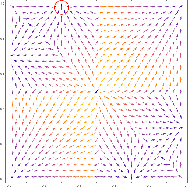
(a) m=30, p=0.3

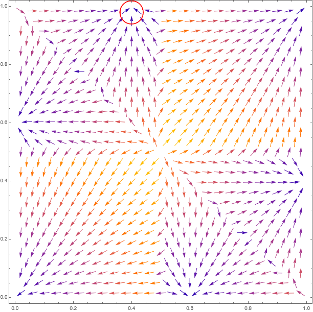
(b) m=40, p=0.4

Figure 4. The vector fields generated by (13) for $p<1/2$ and large m

1.2.2. Continuous-time construction with time delays

The main technique we use to prove Theorem 1.7 is continuous-time embedding. As is mentioned in Remark 1.5, the case $d=1$ was solved by a continuous-time construction. It is natural to consider whether this technique can be generalized.

For the purpose of the proof, we introduce a new time-lines representation which we call continuous-time construction with time delays.

(18)

We let $G$ be a graph as in (18) consisting of a single vertex $x$ and $N_{C}\geq 2$ self-loops, i.e. the edge set $E=\{e_{1},e_{2}.\cdots,e_{N_{c}}\}$ and $x\stackrel{{\scriptstyle e_{i}}}{{\sim}}x$, $i=1,2,\cdots,N_{c}$. We define a continuous-time jump process $X=(X_{t})_{t\geq 0}$ on $G$. Let $0=\tau_{0}<\tau_{1}<\tau_{2}<\cdots$ be the hitting times of $X$ to $x$. For each $i\in\{1,2,\cdots,N_{c}\}$, let

$$Z_{n}(i):=\sum_{k=0}^{n}\mathds{1}_{\left\{(X_{\tau_{k-1}},X_{\tau_{k}})=e_{i}\right\}}+a_{i}$$

be the number of visits to $e_{i}$ up to time $\tau_{n}$ plus $a_{i}\in\mathbb{N}^{+}$. Here $Z_{dn}(i)$ and $a_{i}$ should be interpreted respectively as the number of balls of the $i$-th color in the urn at time $n$ and the initial number of balls of the $i$-th color (see Proposition 1.15 for a more precise statement). For $n\geq a_{i}$, let

(19) $$\sigma_{n}(i):=\inf\{\tau_{m}:Z_{m}(i)\geq n\}$$

with the convention that $\inf\emptyset=\infty$. Let $\{\xi^{(i)}_{n}\}_{1\leq i\leq N_{c},n>a_{i}}$ be independent Exp(1)-distributed random variables. The law of $X$ is defined as follows:

At time $t=0$, for each edge $e_{i}$, $1\leq i\leq N_{c}$, we launch a timer with a duration $\xi^{(i)}_{a_{i}+1}/W(a_{i})$. When the timer of an edge $e_{i}$ rings, $X$ jumps to cross $e_{i}$ instantaneously. If an edge $e_{i}$ is crossed at time $\tau_{n}$ such that $kd<n\leq(k+1)d$ for some $k\in\mathbb{N}$, then we launch a new timer on this edge with a duration $\xi^{(i)}_{Z_{n}(i)+1}/W(Z_{kd}(i))$. At hitting times $\tau_{kd}$, $k\in\mathbb{N}^{+}$, we update the denominators (rates) for all the timers: for $i\in\{1,2,\cdots,N_{c}\}$, if the timer on $e_{i}$ has run a time of $t^{(i)}_{k}$, then we reset the timer such that the remaining time becomes

(20) $$\frac{\xi^{(i)}_{Z_{kd}(i)+1}-W(Z_{(k-1)d}(i))t^{(i)}_{k}}{W(Z_{kd}(i))}$$

Remark 1.8.

(i) Just before we reset the timers, the remaining time of the timer on $e_{i}$ is

$$\frac{\xi^{(i)}_{Z_{kd}(i)+1}}{W(Z_{(k-1)d}(i))}-t^{(i)}_{k}$$

(ii) If, for some $j\in\{1,2,\cdots,N_{c}\}$, $e_{j}$ is not crossed during the time interval $(\tau_{(k-1)d},\tau_{kd}]$, then $Z_{(k-1)d}(j)=Z_{kd}(j)$ so that there is nothing to change for the timer on $e_{j}$.

(iii) If $X$ jumps to cross $e_{j}$ for some $j\in\{1,2,\cdots,N_{c}\}$ at time $\tau_{kd}$, we will launch a new timer on $e_{j}$ and thus $t^{(j)}_{k}=0$. We may simply launch a new timer on $e_{j}$ with a duration $\xi^{(j)}_{Z_{kd}(j)+1}/W(Z_{kd}(j))$ rather than $\xi^{(j)}_{Z_{kd}(j)+1}/W(Z_{(k-1)d}(j))$.

(iv) The timer which corresponds to $\xi^{(i)}_{n+1}$ may run at different rates as time changes. All the possible denominators (rates) are

$$W(n-\ell),\quad\ell\in\{0,1,\cdots,d-1\}\ \text{such that}\ \ell\leq n-a_{i}$$

due to the time delays. Note that we may update this timer at jumping times but we will never launch a new one until it rings. Recall $\sigma_{n}(i)$ defined in (19). If $\sigma_{n+1}(i)<\infty$, the total time this timer needs to run is simply $\sigma_{n+1}(i)-\sigma_{n}(i)$, in which case we can write

(21) $$\sigma_{n+1}(i)-\sigma_{n}(i)=\sum_{\ell=0}^{(d-1)\wedge(n-a_{i})}\frac{b_{\ell}}{W(n-\ell)}$$

where $b_{\ell}\geq 0$ and $\sum_{\ell=0}^{(d-1)\wedge(n-a_{i})}b_{\ell}=\xi^{(i)}_{n+1}$.

We denote the natural filtration of $X$ by $(\mathcal{F}_{t})_{t\geq 0}$, i.e. $\mathcal{F}_{t}:=\sigma(X_{s}:0\leq s\leq t)$.

Proposition 1.15.

Let $X$ be the jump process defined above. Then,

$$(Z_{kd}(i))_{1\leq i\leq N_{c},k\in\mathbb{N}}\stackrel{{\scriptstyle\mathcal{L}}}{{=}}(N_{k}(i))_{1\leq i\leq N_{c},k\in\mathbb{N}}$$

In particular, we may define $X$ and the IUM on the same probability space such that

(22) $$(Z_{kd}(i))_{1\leq i\leq N_{c},k\in\mathbb{N}}=(N_{k}(i))_{1\leq i\leq N_{c},k\in\mathbb{N}}$$

Proof.

Note that conditional on $\mathcal{F}_{\tau_{kd}}$, by the memoryless property of exponentials, (20) has the same distribution as $\xi/W(Z_{kd}(i))$ where $\xi$ is an Exp(1)-distributed random variable. The rest of the proof is similar to that of Lemma 3.1 in [23]. ∎

As we explained in Remark 1.8, unlike the continuous-time construction in the proof of Theorem 3.6 [20], at time $\tau_{n}\in(\tau_{kd},\tau_{(k+1)d})$, we keep using the data we collect at time $\tau_{kd}$ (i.e. $(Z_{kd}(i))_{1\leq i\leq N_{c}}$) to launch new timers. This justifies its name continuous-time construction with time delays. It is a powerful technique that allows us to give a very short proof of a multi-color ($N_{c}\geq 2$) version of Theorem 1.6.

A new proof of Theorem 1.6 with $N_{c}\geq 2$.

Since $\{W_{n}\}$ is non-decreasing, by the conditional Borel-Cantelli lemma, see e.g. [9], a.s. there is a sequence of finite stopping times $\{\tau_{n_{k}d}\}_{k\geq 1}$ such that at time $\tau_{n_{k}d}$, there exists some $i_{k}\in\{1,2,\cdots,N_{c}\}$,

(23) $$Z_{n_{k}d}(i_{k})\geq d+\max_{j\neq i_{k}}\{Z_{n_{k}d}(j)\}$$

Indeed, conditional on $\mathcal{F}_{nd}$, if $Z_{nd}(i)=\max_{1\leq j\leq N_{c}}\{Z_{nd}(j)\}$ for some $i$, the probability that $Z_{(n+1)d}(i)=Z_{nd}(i)+d$ (i.e. we add d balls of the relative major color at time n+1) is lower bounded by $(1/N_{c})^{d}$. Thus, almost surely such an event occurs for infinitely many $n$, which implies (23). By (21), for $j=1,2,\cdots,N_{c}$, if $\sigma_{n}(j)<\infty$,

(24) $$\frac{\xi_{n}^{(j)}}{W(n-1)}\leq\sigma_{n}(j)-\sigma_{n-1}(j)\leq\frac{\xi_{n}^{(j)}}{W(n-d)},\quad\forall n\geq a_{j}+d$$

As is mentioned in the proof of Proposition 1.15, conditional on $\mathcal{F}_{\tau_{n_{k}d}}$, the remaining time of the timer on $e_{j}$ has the distribution of an independent copy of $\xi/W(Z_{n_{k}d}(j))$ where $\xi$ is an Exp(1)-distributed random variable. By a slight abuse of notation, the time remaining is denoted by $\xi^{(j)}_{Z_{n_{k}d}(j)+1}/W(Z_{n_{k}d}(j))$. By symmetry and (23), conditional on $\mathcal{F}_{\tau_{n_{k}d}}$, with probability at least $1/N_{c}$,

$$\sum_{n=Z_{n_{k}d}(i_{k})+1}^{\infty}\frac{\xi_{n}^{(i_{k})}}{W(n-d)}<\min_{j\neq i_{k}}\{\sum_{n=Z_{n_{k}d}(j)+1}^{\infty}\frac{\xi_{n}^{(j)}}{W(n-1)}\}$$

(note that the $N_{c}$ sums above all have continuous distributions) and in particular, by (24),

$$\lim_{n\to\infty}\sigma_{n}(i_{k})-\tau_{n_{k}d}<\min_{j\neq i_{k}}\{\lim_{n\to\infty}\sigma_{n}(j)-\tau_{n_{k}d}\}$$

That is, the remaining time needed to visit $e_{i_{k}}$ i.o. is strictly less than that needed for any other edge. By (22) in Proposition 1.15, this is equivalent to saying that only balls of color $i_{k}$ are taken infinitely often (after time $n_{k}$). Therefore, for any $k\geq 1$,

$$\mathbb{P}_{1}^{W}(\mathcal{M}|\mathcal{F}_{\tau_{n_{k}d}})\geq\frac{1}{N_{c}},\quad\forall k\geq 1$$

We conclude that $\mathbb{P}_{1}^{W}(\mathcal{M})=1$ by Levy’s 0=1 law. ∎

In general, if we do not assume that $\{W(n)\}$ is non-decreasing, by (21), (24) should be replaced by

$$\frac{\xi_{n}^{(j)}}{\max(W(n-\ell):1\leq\ell\leq d\wedge(n-a_{j}))}\leq\sigma_{n}(j)-\sigma_{n-1}(j)\leq\frac{\xi_{n}^{(j)}}{\min(W(n-\ell):1\leq\ell\leq d\wedge(n-a_{j}))}$$

for any $n>a_{j}$ with $\sigma_{n}(j)<\infty$. Moreover, (24) still holds up to small error terms if $|\frac{1}{W(n+1)}-\frac{1}{W(n)}|$ is small for all large $n$ (e.g. if (9) is satisfied) . We use this idea to prove Theorem 1.7 in Section 3.

1.2.3. Coupling

For polynomial reinforcement, we may reduce the problem of monopoly to the problem of domination by coupling.

Assume that we are given 2 urns of black and red balls. Let $(B_{n},R_{n})_{n\in\mathbb{N}}$ be an IUM with reinforcement sequence $\{W(n)\}_{n\in\mathbb{N}}$ and interaction parameter $p$. We define a new urn process $(\tilde{B}_{n},\tilde{R}_{n})_{n\in\mathbb{N}}$ as follows.

As before, we denote by $\tilde{B}_{n}(i)$ and $\tilde{R}_{n}(i)$ ($i=1,2$), respectively, the number of black and red balls in the $i$-th urn at time $n$. Denote $\tilde{B}_{n}:=(\tilde{B}_{n}(1),\tilde{B}_{n}(2))$, $\tilde{R}_{n}:=(\tilde{R}_{n}(1),\tilde{R}_{n}(2))$ and $\tilde{B}_{n}^{*}:=\tilde{B}_{n}(1)+\tilde{B}_{n}(2)$, $\tilde{R}_{n}^{*}:=\tilde{R}_{n}(1)+\tilde{R}_{n}(2)$. At time 0, the initial composition is given by $(\tilde{B}_{0},\tilde{R}_{0})\in\mathbb{N}^{4}$. For any $n\in\mathbb{N}$, at time $2n+1$, we add a black ball to the first urn with probability

$$\frac{W(\tilde{B}_{2n}(1))}{W(\tilde{B}_{2n}(1))+W(\tilde{R}_{2n}^{*})}$$

or we add a red ball otherwise; at time $2n+2$, we add a black ball to the second urn with probability

$$\frac{W(\tilde{B}_{2n}(2))}{W(\tilde{B}_{2n}(2))+W(\tilde{R}_{2n+1}^{*})}$$

or we add a red ball otherwise.

Lemma 1.16.

Assume that $\{W(n)\}_{n\in\mathbb{N}}$ is non-decreasing and $(\tilde{B}_{0},\tilde{R}_{0})=(B_{0},R_{0})$. Then we can define the two urn processes $(B_{n},R_{n})_{n\in\mathbb{N}}$ and $(\tilde{B}_{n},\tilde{R}_{n})_{n\in\mathbb{N}}$ above on the same probability space such that

(25) $$\tilde{R}_{2n}(i)\geq R_{n}(i),\ \tilde{B}_{2n}(i)\leq B_{n}(i),\quad\forall n\in\mathbb{N},i=1,2$$

Note that in Lemma 1.16, we do not assume that $\{W(n)\}$ is polynomial. Now we consider polynomial reinforcement.

Lemma 1.17.

Assume that $W(n)=n^{m}$, $n\in\mathbb{N}$, where $m\geq 2$. For any $\varepsilon>0$, there exists positive constants $\varepsilon_{1}\in(0,1),\kappa\in\mathbb{N}^{+}$ such that if $n\geq\kappa$ and $\tilde{R}_{2n}^{*}<\varepsilon_{1}n$, then

$$\mathbb{P}(\lim_{\ell\to\infty}\tilde{R}^{*}_{\ell}<\infty|\tilde{\mathcal{F}}_{2n})>1-\varepsilon$$

where $\tilde{\mathcal{F}}_{n}:=\sigma(\tilde{B}_{m}(i),\tilde{R}_{m}(i):1\leq i\leq 2,m\leq n)$

Using Lemma 1.16 and Lemma 1.17, we can prove Proposition 1.5.

Proof of Proposition 1.5.

Fix $\varepsilon\in(0,1)$, let $\varepsilon_{1},\kappa$ be as in Lemma 1.17. Define $T_{0}=\kappa$ and for any $n\in\mathbb{N}$,

$$T_{n+1}:=\inf\{m>T_{n}:\min(B^{*}_{m},R^{*}_{m})<\varepsilon_{1}m\}$$

with the convention that $\inf\emptyset=\infty$. If $T_{n}=\infty$, we set $T_{k}:=\infty$ for all $k>n$. Then $\{T_{n}\}_{n\in\mathbb{N}}$ is an infinite sequence of stopping times. By Lemma 1.16 and Lemma 1.17, for any $n\geq 1$,

$$\mathbb{P}_{p}^{(m)}(\mathcal{D}^{c}\cup\mathcal{M}|\mathcal{F}_{T_{n}})\mathds{1}_{\{T_{n}<\infty\}}\geq\mathbb{P}_{p}^{(m)}(\mathcal{M}|\mathcal{F}_{T_{n}})\mathds{1}_{\{T_{n}<\infty\}}\geq(1-\varepsilon)\mathds{1}_{\{T_{n}<\infty\}}$$

On the other hand, since $\{T_{n}=\infty\}\subset\mathcal{D}^{c}$,

$$\mathbb{P}_{p}^{(m)}(\mathcal{D}^{c}\cup\mathcal{M}|\mathcal{F}_{T_{n}})\mathds{1}_{\{T_{n}=\infty\}}=\mathds{1}_{\{T_{n}=\infty\}}$$

Thus, for any $n\geq 1$,

$$\mathbb{P}_{p}^{(m)}(\mathcal{D}^{c}\cup\mathcal{M}|\mathcal{F}_{T_{n}})>1-\varepsilon$$

By Levy’s 0-1 law. $\mathbb{P}(\mathcal{D}^{c}\cup\mathcal{M})=1$ which completes the proof since $\mathcal{M}\subset\mathcal{D}$. ∎

1.3. Organization of the paper

In Section 2, we prove Proposition 1.10, Theorem 1.2, Theorem 1.4 and Proposition 1.3. Theorem 1.7 is proved in Section 3. Section 4 is devoted to the proofs of Lemma 1.16 and Lemma 1.17.

Some open problems are presented in the last section.

2. Stochastic approximation algorithm

Proof of Proposition 1.10.

It is direct to check that $(0,0),(1/2,1/2),(1,1)$ belong to $\Lambda^{(m)}$. If $z\in[1/2,1]$,

(26) $$\frac{z^{m}}{z^{m}+(1-z)^{m}}=\frac{1}{1+(\frac{1}{z}-1)^{m}}\geq\frac{1}{1+(\frac{1}{z}-1)}=z$$

where the equality holds if and only if $z=1/2$ or $z=1$. The inequality (26) is reversed if $z\in[0,1/2]$ where the equality holds if and only if $z=0$ or $z=1/2$. In particular, if $p=0$, $\Lambda^{(m)}=\{0,1/2,1\}\times\{0,1/2,1\}$. We assume that $p>0$. If $(x,y)\in[1/2,1]^{2}$ is a equilibrium, then by (26), we have

$$0=-x+\frac{(1-p)x^{m}}{x^{m}+(1-x)^{m}}+\frac{p(x+y)^{m}}{(x+y)^{m}+(2-x-y)^{m}}\geq-x+(1-p)x+p\frac{x+y}{2}=\frac{p(y-x)}{2}$$

and similarly

$$0=-y+\frac{(1-p)y^{m}}{y^{m}+(1-y)^{m}}+\frac{p(x+y)^{m}}{(x+y)^{m}+(2-x-y)^{m}}\geq\frac{p(x-y)}{2}$$

Thus, $(x,y)=(1/2,1/2)$ or $(1,1)$. Similarly, if $(x,y)\in[0,1/2]^{2}$ is a equilibrium, then $(x,y)=(0,0)$ or $(1/2,1/2)$. Moreover, it is easy to see that if $(x,y)\in\partial[0,1]^{2}$ is a equilibrium, then $(x,y)=(0,0)$ or $(1,1)$. Now it remains to show that $\Lambda^{(m)}$ is a finite set if $p>0$. In the proof of Proposition 2.2 (see Claim 1), we will show that $\Lambda^{(m)}$ is a finite set if $p\geq 1/2$. Now we assume that $0<p<1/2$. Observe that if $(x,y)\in\Lambda^{(m)}$, $(1-x,1-y)\in\Lambda^{(m)}$. Therefore, it suffices to prove the following claim.

Claim: The set $\{(x,y)\in\Lambda^{(m)}:0<x<1/2<y<1,x+y\geq 1\}$ is finite.

Proof of the claim: Let

(27) $$g_{1}(t):=t-\frac{(1-p)t^{m}}{t^{m}+(1-t)^{m}},\quad t\in[0,1]$$

Then, $g_{1}^{\prime}(t)=1-m(1-p)f(t)$ where $f$ is defined in (14). Note that $g_{1}(0)=0,g_{1}(1/2)=p/2,g_{1}(1)=p$. $f$ is increasing on $[0,1/2]$ and decreasing on $[1/2,1]$, and thus $g$ is concave on $[0,1/2]$ and convex on $[1/2,1]$. Since $p<1/2$,

$$g_{1}^{\prime}(\frac{1}{2})=1-m(1-p)<1-\frac{m}{2}\leq 0,\quad g_{1}^{\prime}(1)=1$$

and thus $g(t)$ is decreasing on $[1/2,t_{0}]$ and increasing on $[t_{0},1]$ for some $t_{0}\in(1/2,1)$. Since $g_{1}(t_{0})<p/2$, there exists $\varepsilon>0$ such that for $z\in(1/2-\varepsilon,1]$,

(28) $$g_{2}(z):=\frac{pz^{m}}{z^{m}+(1-z)^{m}}>g_{1}(t_{0})$$

and thus, there exists a unique $y\in(t_{0},1]$ such that $g_{1}(y)=g_{2}(z)$. Note that at this $y$, $g_{1}^{\prime}(y)>0$. By the analytic implicit function theorem, see e.g. Theorem 6.1.2 [15], we may denote the solution by $y=h(z)$, $z\in(1/2-\varepsilon,1]$, where $h$ is analytic on $(1/2-\varepsilon,1)$ with

(29) $$h^{\prime}(z)=\frac{pmf(z)}{1-m(1-p)f(h(z))},\quad h(\frac{1}{2})>t_{0},\quad h(1)=1$$

Note that the denominator is positive since $g_{1}^{\prime}(h(z))>0$ as we mentioned above. Observe that $2-h^{\prime}(z)$ is increasing on $[1/2,1)$ and $1-h(1/2)<1$. Thus, for $z\in[1/2,1)$,

(30) $$0<1-h(z)\leq 2z-h(z)<2-h(1)=1$$

Moreover, $2z-h(z)\to 1$ when $z$ increases to 1. Now we consider the analytic function $g_{3}(z):=g_{1}(2z-h(z))-g_{2}(z)$ on $(1/2-\varepsilon,1)$. It is non-constant since its derivative

(31) $$g_{3}^{\prime}(z)=(1-m(1-p)f(2z-h(z)))(2-h^{\prime}(z))-mpf(z)$$

converges to 2 as $z\to 1$ ($f(z)\to 0$ as $z\to 1$). As a non-constant analytic function, $g_{3}$ has finite zeros on $[1/2,3/4]$. Observe that if $(x,y)\in\Lambda^{(m)}$ with $0<x<1/2<y<1$ and $z:=(x+y)/2\geq 1/2$, then $z$ is a zero of $g_{3}(z)$ on $[1/2,3/4]$ with $y=h(z)$ and $x=2z-h(z)$, which completes the proof of the claim. ∎

Proof of Theorem 1.2.

By Proposition 1.12, $(x_{n},y_{n})$ converges a.s.. It suffices to prove the second assertion. For $p<1/2$, define a function $g$ by

$$g(u):=-u+\frac{(1-p)u^{m}}{u^{m}+(1-u)^{m}}+\frac{p}{2},\quad u\in[0,\frac{1}{2}]$$

Let $f$ be as in (14). Then, $g(0)=p/2,g(1/2)=0$ and

$$g^{\prime}(u)=-1+m(1-p)f(u),\quad u\in[0,\frac{1}{2}]$$

is an increasing function on $[0,1/2]$, and $g^{\prime}(1/2)=m(1-p)-1>0$. Thus, there exists a unique solution $u_{m}\in[0,1/2)$ to the equation $g(u)=0$. Note that $u_{m}=0$ only when $p=0$.
Claim: There exists $q_{m}>0$ such that if $p<q_{m}$, $(u_{m},1-u_{m})\in\mathcal{E}_{s}^{(m)}$, i.e.

$$\lambda_{+}(u_{m},1-u_{m})<0$$

where $\lambda_{+}$ is defined in (15). Once this claim is proved, by Proposition 1.13, $\mathbb{P}_{p}^{(m)}((x_{n},y_{n})\to(u_{m},1-u_{m}))$ is positive, which completes the proof of Theorem 1.2.
Proof of the claim. Note that $f(1/2)=1$ and $f(u_{m})=f(1-u_{m})$. By (15), we need to prove that for $p<q_{m}$,

(32) $$-1+mp+m(1-p)f(u_{m})<0$$

For $p=0$ (and thus $u_{m}=0$), (32) is obvious. For $p>0$, $u_{m}>0$. Moreover, using that $g(u_{m})=0$ (and thus $g(1-u_{m})=0$), we have

$$\frac{u_{m}^{m-1}}{u_{m}^{m}+(1-u_{m})^{m}}=\frac{u_{m}-\frac{p}{2}}{(1-p)u_{m}},\quad\frac{(1-u_{m})^{m-1}}{u_{m}^{m}+(1-u_{m})^{m}}=\frac{1-u_{m}-\frac{p}{2}}{(1-p)(1-u_{m})}$$

Thus, by the definition (14),

$$f(u_{m})=\frac{(u_{m}-\frac{p}{2})(1-u_{m}-\frac{p}{2})}{(1-p)^{2}u_{m}(1-u_{m})}$$

Then (32) is equivalent to

(33) $$u_{m}<\frac{1}{2}-\frac{1}{2}\sqrt{\frac{(m-1)(1-p)}{m-1+p+mp-mp^{2}}}$$

As discussed above, fix $m$, for any $p\in[0,1/2)$, there exists a unique $u_{m}=u_{m}(p)$ such that

$$G(u_{m},p):=-u_{m}+\frac{(1-p)u_{m}^{m}}{u_{m}^{m}+(1-u_{m})^{m}}+\frac{p}{2}=0$$

Since $\partial_{p}G(0,0)\neq 0$, by the implicit function theorem, we can extend $u_{m}(p)$ to $(-\varepsilon,1/2)$ for some $\varepsilon>0$ such that $u_{m}(p)$ is the unique diffentiable function satisfying $G(u_{m}(p),p)=0$ on $(-\varepsilon,1/2)$. Moreover,

$$-u_{m}^{\prime}(0)+\frac{1}{2}=u_{m}^{\prime}(0)g^{\prime}(0)+\frac{1}{2}=0$$

whence $u_{m}^{\prime}(0)=1/2$. Now, we consider the function $h(p)$ defined by

$$h(p):=\frac{1}{2}-\frac{1}{2}\sqrt{\frac{(m-1)(1-p)}{m-1+p+mp-mp^{2}}},\quad p\in[0,1/2)$$

Then, $h(0)=0=u_{m}(0)$ and $h^{\prime}(0)=m/(2(m-1))>1/2=u_{m}^{\prime}(0)$. Thus, (33) is true if $p\in(0,q_{m})$ for some $q_{m}>0$. ∎

To prove Theorem 1.4, we need the following auxiliary lemma.

Lemma 2.1.

For any $h\in(0,1/\sqrt{5})$ and $m\geq 3$, we have

$$\frac{(1+h)^{m}-(1-h)^{m}}{(1+h)^{m}+(1-h)^{m}}\geq 2h$$

Proof.

We need to show that

$$(\frac{1+h}{1-h})^{m}\geq\frac{1+2h}{1-2h},\quad h\in(0,\frac{1}{\sqrt{5}})$$

Note that we only need to prove the case $m=3$ since the left-hand side is increasing in $m$. Now observe that if $h\in(0,1/\sqrt{5})$,

$$(1-2h)(1+h)^{3}-(1+2h)(1-h)^{3}=2h(1-5h^{2})\geq 0$$

which completes the proof. ∎

Proposition 2.2.

For any $m\geq 2$, $p_{m}<1/2$.

Proof.

Note that $(0,1),(1,0)\notin\Lambda^{(m)}$. If $p\geq 1/2$ and $(x,y)\in\Lambda^{(m)}$ with $x+y=1$, then

$$\lambda_{+}(x,y)=-1+mp+m(1-p)f(x)>mp-1\geq 0$$

Thus, all the equilibria on the line $x+y=1$ are unstable if $p\geq 1/2$. Note that there are only finitely many equilibria on the line $x+y=1$.

Claim 1: If $p\geq 1/2$, except $(0,0),(1,1)$ and (finitely many unstable) equilibria on the line $x+y=1$, there are no other equilibria. In particular, $\mathbb{P}_{p}^{(m)}(\mathcal{D})=1$ by Proposition 1.12 and Proposition 1.14.
Proof of Claim 1: By symmetry, as in the proof of Proposition 1.10, it suffices to prove that there is no equilibrium $(\tilde{x},\tilde{y})$ such that $0<\tilde{x}<1/2<\tilde{y}<1$ and $\tilde{z}:=(\tilde{x}+\tilde{y})/2\in(1/2,3/4)$. We argue by contradiction. Since $(\tilde{x},\tilde{y})\in\Lambda^{(m)}$,

(34) $$-2\tilde{z}+(1-p)\frac{(2\tilde{z}-\tilde{y})^{2}}{(2\tilde{z}-\tilde{y})^{2}+(1+\tilde{y}-2\tilde{z})^{2}}+(1-p)\frac{\tilde{y}^{2}}{\tilde{y}^{2}+(1-\tilde{y})^{2}}+2p\frac{\tilde{z}^{2}}{\tilde{z}^{2}+(1-\tilde{z})^{2}}=0$$

Now fix $z\in(1/2,3/4)$, the function

$$J(y):=\frac{(2z-y)^{m}}{(2z-y)^{m}+(1+y-2z)^{m}}+\frac{y^{m}}{y^{m}+(1-y)^{m}},\quad y\in[2z-\frac{1}{2},1]$$

has derivative $J^{\prime}(y)=-m(f(2z-y)-f(y))$ where $f$ is defined in (14). Observe that $|2z-y-1/2|\leq y-1/2$ and thus $J^{\prime}(y)\leq 0$. In particular, for any $y\in[2z-\frac{1}{2},1]$,

(35) $$\quad-2z+(1-p)\frac{(2z-y)^{m}}{(2z-y)^{m}+(1+y-2z)^{m}}+(1-p)\frac{y^{2}}{y^{2}+(1-y)^{2}}+2p\frac{z^{m}}{z^{m}+(1-z)^{m}}$$

$$\geq-2z+(1-p)\frac{(2z-1)^{2}}{(2z-1)^{2}+(2-2z)^{2}}+(1-p)+2p\frac{z^{m}}{z^{m}+(1-z)^{m}}$$

We claim that for any $z\in(1/2,3/4)$,

(36) $$-2z+(1-p)\frac{(2z-1)^{m}}{(2z-1)^{2}+(2-2z)^{m}}+(1-p)+2p\frac{z^{m}}{z^{m}+(1-z)^{m}}>0$$

which contradicts (34) by (35), and thus implies Claim 1.
Proof of (36): First note that

(37) $$\frac{2z^{m}}{z^{m}+(1-z)^{m}}-1-\frac{(2z-1)^{m}}{(2z-1)^{m}+(2-2z)^{m}}\geq 0$$

Indeed, it is equivalent to

$$[z^{m}-(1-z)^{m}][(2z-1)^{2}+(2-2z)^{m}]-[z^{m}+(1-z)^{m}](2z-1)^{m}\geq 0$$

The left-hand side equals

$$(2-2z)^{m}[z^{m}-2(z-\frac{1}{2})^{m}-(1-z)^{m}]$$

Let $v:=z-1/2\in(0,1/4)$,

$$z^{m}-2(z-\frac{1}{2})^{m}-(1-z)^{m}=(\frac{1}{2}+v)^{m}-(\frac{1}{2}-v)^{m}-2v^{m}\geq\frac{2mv}{2^{m-1}}-2v^{m}\geq 0$$

which completes the proof of (37). Thus, the left-hand side of (36) is an increasing function in $p$. It suffices to prove the case $p=1/2$, i.e. we need to show that for any $v\in(0,1/4)$,

$$-2v-\frac{1}{2}+\frac{1}{2}\frac{(2v)^{m}}{(2v)^{m}+(1-2v)^{m}}+\frac{(\frac{1}{2}+v)^{m}}{(\frac{1}{2}+v)^{m}+(\frac{1}{2}-v)^{m}}>0$$

Let $h=2v\in(0,1/2)$, it is equivalent to proving that for any $h\in(0,1/2)$, $\beta(h)>0$ where

(38) $$\beta(h):=\frac{1}{2}\frac{(1+h)^{m}-(1-h)^{m}}{(1+h)^{m}+(1-h)^{m}}+\frac{1}{2}\frac{h^{m}}{h^{m}+(1-h)^{m}}-h,\quad h\in(0,\frac{1}{2})$$

First, observe that

$$\beta(h)=-g(\frac{1-h}{2})+\frac{1}{2}g(h)+\frac{1}{2}-h$$

where

$$g(t):=\frac{t^{m}}{t^{m}+(1-t)^{m}},\quad t\in[0,1]$$

For $t\in[0,1/2]$, we have

$$\frac{1}{2}g(t)=\frac{1}{2}\frac{t^{m}}{t^{m}+(1-t)^{m}}\geq\frac{1}{2^{\frac{m}{2}}}\frac{t^{m}}{(\frac{t}{\sqrt{2}})^{m}+(1-\frac{t}{\sqrt{2}})^{m}}=g(\frac{t}{\sqrt{2}})$$

If $1/(1+\sqrt{2})\leq h\leq 1/2$, then $h/\sqrt{2}\geq(1-h)/2$ and thus by the monotonicity of $g$,

$$\beta(h)\geq-g(\frac{1-h}{2})+g(\frac{h}{\sqrt{2}})+\frac{1}{2}-h\geq 0$$

On the other hand, by Lemma 2.1, if $0<h<1/(1+\sqrt{2})<1/\sqrt{5}$ and $m\geq 3$, then $\beta(h)>0$. When $m=2$, for $h\in(0,1/2)$,

$$\beta(h)=\frac{h}{1+h^{2}}-h+\frac{h^{2}}{4h^{2}-4h+2}=\frac{h^{2}(1-2h+h^{2}(5-4h))}{(1+h^{2})(4h^{2}-4h+2)}>0$$

which completes the proof of (36) and Claim 1.

Now we prove that $p_{m}<1/2$. We argue by contradiction: fix $m\geq 2$, assume that for any $q<1/2$, there exist $p\in(q,1/2)$ such that $\mathbb{P}_{p}^{(m)}(\mathcal{D})<1$. Then, by Proposition 1.10, Proposition 1.12 and Proposition 1.14, there exist sequences $\{p^{(k)}\}_{k\geq 1}$ and $\{s_{k}\}_{k\geq 1}$ such that for any $k\geq 1$,

$$0<p^{(k)}<1/2,\quad s_{k}=(s_{k}(1),s_{k}(2))\in\Lambda^{(m)}\backslash([0,1/2]^{2}\cup[1/2,1]^{2})\ \text{with}\ \lambda_{+}(s_{k})\leq 0$$

and

$$\lim_{k\to\infty}p^{(k)}=\frac{1}{2},\quad\mathbb{P}_{p^{(k)}}^{(m)}(\lim_{n\to\infty}(x_{n},y_{n})=(s_{k}(1),s_{k}(2)))>0$$

Since $[0,1]^{2}$ is compact, by possibly choosing a subsequence, we may assume that

$$\lim_{k\to\infty}(p^{(k)},s_{k})=(\frac{1}{2},s)$$

where $s\notin\{(0,0),(1,1)\}$. Since $F^{(m)}$ and $\lambda_{+}$ are continuous function in $(p,x,y)$, we see that $F^{(m)}(s)=0$ and $\lambda_{+}(s)\leq 0$ with $p=1/2$, which contradicts Claim 1. ∎

Combined with Proposition 2.2, the following proposition implies Theorem 1.4.

Proposition 2.3.

If $p<1/2$, then for large $m$, there exists an $s_{m}\in\mathcal{E}_{s}^{(m)}$ such that $\lim_{m\to\infty}s_{m}=(p,1)$. In particular, for $\mathbb{P}_{p}^{(m)}$, with positive probability, $\lim_{n\to\infty}(x_{n},y_{n})=s_{m}$.

Proof.

We use the notations from the proof of Proposition 1.10. Recall $g_{1},g_{2}$ defined in (27) and (28), respectively. The function $h(z):[1/2,1]\to(t_{0},1]$ satisfies $g_{1}(h(z))=g_{2}(z)$. By (26), if $z\in(1/2,1)$, then

$$g_{1}(z)<g_{2}(z)=g_{1}(h(z))$$

Since $g_{1}$ is increasing on $(t_{0},1]$, $h(z)>z$ for $z\in(1/2,1)$. Therefore, fix a small $\delta>0$, for any $z\geq 1/2+\delta$,

$$h(z)=\frac{(1-p)h(z)^{m}}{h(z)^{m}+(1-h(z))^{m}}+g_{2}(z)\geq\frac{z^{m}}{z^{m}+(1-z)^{m}}\geq\frac{(1/2+\delta)^{m}}{(1/2+\delta)^{m}+(1/2-\delta)^{m}}\to 1$$

uniformly as $m\to\infty$. We choose a large $m$ such that $h(z)>1-\delta$ for any $z\geq 1/2+\delta$. Now consider the function $g_{3}(z):=g_{1}(2z-h(z))-g_{2}(z)$. As in (30), since $2z-h(z)$ is convex on $[1/2+\delta,3/4-\delta]$, for any $z\in[1/2+\delta,3/4-\delta]$,

(39) $$0<2z-h(z)<\frac{1}{2}-\delta$$

Using (31), (29), (39), and that

(40) $$mf(t)=\frac{mt^{m-1}(1-t)^{m-1}}{(t^{m}+(1-t)^{m})^{2}}\to 0,\quad\text{as}\ m\to\infty$$

uniformly on $[0,1/2-\delta]\cup[1/2+\delta,1]$, we have

(41) $$\lim_{m\to\infty}g_{3}^{\prime}(z)=2,\quad\text{uniformly on}\ [\frac{1}{2}+\delta,\frac{3}{4}-\delta]$$

On the other hand,

(42) $$\lim_{m\to\infty}g_{3}(\frac{1}{2}+\delta)=2\delta-p,\quad\lim_{m\to\infty}g_{3}(\frac{3}{4}-\delta)=\frac{1}{2}-2\delta-p$$

We may assume that $2\delta<\min(1/2-p,p)$. By (42), for all large $m$, we have $g_{3}(\frac{1}{2}+\delta)<0$, $g_{3}(\frac{3}{4}-\delta)>0$, and by (41), there exists a unique $z_{m}\in(1/2+\delta,3/4-\delta)$ such that $g_{3}(z_{m})=0$. In particular, $(2z_{m}-h(z_{m}),h(z_{m}))\in\Lambda^{(m)}$. Observe that by (41),

$$\lim_{m\to\infty}z_{m}=\frac{3}{4}-\delta-\frac{1}{2}(\frac{1}{2}-2\delta-p)=\frac{1+p}{2}$$

and thus

$$\lim_{m\to\infty}(2z_{m}-h(z_{m}),h(z_{m}))=(p,1)$$

We claim that $s_{m}:=(2z_{m}-h(z_{m}),h(z_{m}))$ is strictly stable. Indeed, since none of $2z_{m}-h(z_{m}),z_{m}$ and $h(z_{m})$ are in the interval $[1/2-\delta,1/2+\delta]$, by (40), we have

$$\lim_{m\to\infty}\left(mf(2z_{m}-h(z_{m})),mf(z_{m}),mf(h(z_{m}))\right)=(0,0,0)$$

Thus, by (15),

$$\lim_{m\to\infty}\lambda_{+}(2z_{m}-h(z_{m}),h(z_{m}))=-1$$

Therefore, for all large $m$, we have $\lambda_{+}(2z_{m}-h(z_{m}),h(z_{m}))<0$, i.e. $s_{m}\in\mathcal{E}_{s}^{(m)}$. The last assertion follows from Proposition 1.13. ∎

Proof of Proposition 1.3.

Let $u_{2}$ be as in Theorem 1.2. For $p<1/2$, $u_{2}=u_{2}(p)$ is given by

$$u_{2}(p)=\frac{1}{2}-\frac{\sqrt{1-2p}}{2}$$

(33) then becomes

$$\frac{1}{2}-\frac{\sqrt{1-2p}}{2}<\frac{1}{2}-\frac{1}{2}\sqrt{\frac{1-p}{1+3p-2p^{2}}}$$

which is true if and only if $p<1-\sqrt{2}/2$. Thus, from the proof of Theorem 1.2, we see that $(u_{2},1-u_{2})\in\mathcal{E}_{s}^{(m)}$ if $p<1-\sqrt{2}/2$. It remains to apply Proposition 1.13. ∎

3. Continuous-time construction with time-delays

Let $X$ be the jump process defined in Section 1.2. By Proposition 1.15, we may define $X$ and the IUM $(N_{n})_{n\in\mathbb{N}}$ on the same probability space $(\Omega,\mathcal{F},\mathbb{P})$ such that (22) holds.

Proof of Theorem 1.7.

By (21), for any $j\in\{1,2,\cdots,N_{c}\}$ and $n\geq a_{j}+d-1$, if $\sigma_{n+1}(j)<\infty$, we can write

$$\sigma_{n+1}(j)-\sigma_{n}(j)=\sum_{i=0}^{d-1}\frac{b_{i}}{W(n-i)},$$

where $b_{i}\geq 0$ and $\sum_{i=0}^{d-1}b_{i}=\xi^{(j)}_{n+1}$. Observe that

$$\frac{b_{d-1}}{W(n-d+1)}+\frac{b_{d-2}}{W(n-d+2)}=b_{d-1}(\frac{1}{W(n-d+1)}-\frac{1}{W(n-d+2)})+\frac{b_{d-1}+b_{d-2}}{W(n-d+2)}$$

which belongs to the closed interval

$$\left[\frac{b_{d-1}+b_{d-2}}{W(n-d+2)}-|\frac{\xi^{(j)}_{n+1}}{W(n-d+1)}-\frac{\xi^{(j)}_{n+1}}{W(n-d+2)}|,\frac{b_{d-1}+b_{d-2}}{W(n-d+2)}+|\frac{\xi^{(j)}_{n+1}}{W(n-d+1)}-\frac{\xi^{(j)}_{n+1}}{W(n-d+2)}|\right]$$

Repeating this procedure gives

(43) $$\quad\frac{\xi^{(j)}_{n+1}}{W(n)}-\xi^{(j)}_{n+1}\sum_{i=0}^{d-2}|\frac{1}{W(n-i-1)}-\frac{1}{W(n-i)}|$$

$$\leq\sigma_{n+1}(j)-\sigma_{n}(j)$$

$$\leq\frac{\xi^{(j)}_{n+1}}{W(n)}+\xi^{(j)}_{n+1}\sum_{i=0}^{d-2}|\frac{1}{W(n-i-1)}-\frac{1}{W(n-i)}|$$

By (9), for any $k\geq n$,

(44) $$\frac{W(n)}{W(k)}-1\leq W(n)|\frac{1}{W(k)}-\frac{1}{W(n)}|\leq C$$

In particular, $W(n)/\inf_{k\geq n}W(k)\leq C+1$ for any $n\geq 1$. As in (23), the conditional Borel-Cantelli lemma then implies that a.s. there is a sequence of finite stopping times $\{\tau_{n_{k}d}\}_{k\geq 1}$ such that at time $\tau_{n_{k}d}$, there exists some $i_{k}\in\{1,2,\cdots,N_{c}\}$,

(45) $$Z_{n_{k}d}(i_{k})\geq d+\max_{j\neq i_{k}}\{Z_{n_{k}d}(j)\}$$

As in the proof of Theorem 1.6, by a slight abuse of notation, at time $\tau_{n_{k}d}$, for any $j\in\{1,2,\cdots,N_{c}\}$, the time remaining of the timer on $e_{j}$ is denoted by $\xi^{(j)}_{Z_{n_{k}d}(j)+1}/W(Z_{n_{k}d}(j))$. We assume that $Z_{n_{k}d}(q)=\max_{j\neq i_{k}}\{Z_{n_{k}d}(j)\}$ for some $q\neq i_{k}$. Then,

$$\mathbb{E}\sum_{n=Z_{n_{k}d}(i_{k})}^{\infty}(\xi^{(i_{k})}_{n+1}+\xi^{(q)}_{n+1})\sum_{\ell=0}^{d-2}|\frac{1}{W(n-\ell-1)}-\frac{1}{W(n-\ell)}|=\sum_{n=Z_{n_{k}d}(i_{k})}^{\infty}\sum_{\ell=0}^{d-2}|\frac{2}{W(n-\ell-1)}-\frac{2}{W(n-\ell)}|$$

Note that for each $n\geq Z_{n_{k}d}(i_{k})-d+1$, the term $|\frac{2}{W(n)}-\frac{2}{W(n+1)}|$ is counted at most $d-1$ times in the right-hand side. Thus, by (9),

$$\quad\mathbb{E}\sum_{n=Z_{n_{k}d}(i_{k})}^{\infty}(\xi^{(i_{k})}_{n+1}+\xi^{(q)}_{n+1})\sum_{\ell=0}^{d-2}|\frac{1}{W(n-\ell-1)}-\frac{1}{W(n-\ell)}|$$

$$\leq 2(d-1)\sum_{n=Z_{n_{k}d}(i_{k})-d+1}^{\infty}|\frac{1}{W(n)}-\frac{1}{W(n+1)}|\leq\frac{2C(d-1)}{W(Z_{n_{k}d}(i_{k})-d+1)}$$

By Markov inequality, for any positive random variable $Y$, if $m(Y)$ denotes its median value, then

$$\frac{1}{2}\leq\mathbb{P}(Y\geq m(Y))\leq\frac{\mathbb{E}Y}{m(Y)}$$

and thus $m(Y)\leq 2\mathbb{E}Y$. In particular,

(46) $$\mathbb{P}(\sum_{n=Z_{n_{k}d}(i_{k})}^{\infty}(\xi^{(i_{k})}_{n+1}+\xi^{(q)}_{n+1})\sum_{\ell=0}^{d-2}|\frac{1}{W(n-\ell-1)}-\frac{1}{W(n-\ell)}|\leq\frac{4C(d-1)}{W(Z_{n_{k}d}(i_{k})-d+1)})\geq\frac{1}{2}$$

By (44) and (45), starting from time $\tau_{n_{k}d}$, the time needed to visit $e_{q}$ once more is

(47) $$\sigma_{Z_{n_{k}d}(q)+1}(q)-\sigma_{Z_{n_{k}d}(q)}(q)=\frac{\xi^{(q)}_{Z_{n_{k}d}(q)+1}}{W(Z_{n_{k}d}(q))}\geq\frac{\xi^{(q)}_{Z_{n_{k}d}(q)+1}}{(C+1)W(Z_{n_{k}d}(i_{k})-d+1)}$$

By (45), $\xi^{(q)}_{Z_{n_{k}d}(q)+1}$ is independent of $\{\xi^{(i_{k})}_{n+1},\xi^{(q)}_{n+1}\}_{n\geq Z_{n_{k}d}(i_{k})}$. Therefore, by (46) and that $\xi^{(q)}_{Z_{n_{k}d}(q)+1}\sim\operatorname{Exp}(1)$, conditional on $\mathcal{F}_{\tau_{n_{k}d}}$,

$$\mathbb{P}(E_{q,i})\geq\frac{1}{2}\mathbb{P}(\xi^{(q)}_{Z_{n_{k}d}(q)+1}>4C(d-1)(C+1))\geq\frac{1}{2}e^{-4C(d-1)(C+1)}$$

where the event $E_{q,i}$ is defined by

$$E_{q,i}:=\{\frac{\xi^{(q)}_{Z_{n_{k}d}(q)+1}}{(C+1)W(Z_{n_{k}d}(i)-d+1)}>\sum_{n=Z_{n_{k}d}(i_{k})}^{\infty}(\xi^{(i_{k})}_{n+1}+\xi^{(q)}_{n+1})\sum_{i=0}^{d-2}|\frac{1}{W(n-i-1)}-\frac{1}{W(n-i)}|\}$$

By symmetry of $\{\xi^{(i_{k})}_{n+1}\}_{n\geq Z_{n_{k}d}(i_{k})}$ and $\{\xi^{(q)}_{n+1}\}_{n\geq Z_{n_{k}d}(i_{k})}$, conditional on $\mathcal{F}_{\tau_{n_{k}d}}$, we have

(48) $$\quad\mathbb{P}(\{\sum_{n=Z_{n_{k}d}(i_{k})}^{\infty}\frac{\xi^{(i_{k})}_{n+1}}{W(n)}<\sum_{n=Z_{n_{k}d}(i_{k})}^{\infty}\frac{\xi^{(q)}_{n+1}}{W(n)}\}\cap E_{q,i})=\mathbb{P}(\{\sum_{n=Z_{n_{k}d}(i_{k})}^{\infty}\frac{\xi^{(q)}_{n+1}}{W(n)}<\sum_{n=Z_{n_{k}d}(i_{k})}^{\infty}\frac{\xi^{(i_{k})}_{n+1}}{W(n)}\}\cap E_{q,i})$$

$$=\frac{\mathbb{P}(E_{q,i})}{2}\geq\frac{1}{4}e^{-4C(d-1)(C+1)}$$

For $j\neq i_{k}$, we define $E_{j}$ be the event that

$$\frac{\xi^{(j)}_{Z_{n_{k}d}(j)+1}}{(C+1)W(Z_{n_{k}d}(i_{k})-d+1)}+\sum_{n=Z_{n_{k}d}(i)}^{\infty}\left(\frac{\xi^{(j)}_{n+1}}{W(n)}-\xi^{(j)}_{n+1}\sum_{\ell=0}^{d-2}|\frac{1}{W(n-\ell-1)}-\frac{1}{W(n-\ell)}|\right)$$

$$>\sum_{n=Z_{n_{k}d}(i_{k})}^{\infty}\frac{\xi^{(i_{k})}_{n+1}}{W(n)}+\xi^{(i_{k})}_{n+1}\sum_{\ell=0}^{d-2}|\frac{1}{W(n-\ell-1)}-\frac{1}{W(n-\ell)}|$$

Then by symmetry and (48), conditional on $\mathcal{F}_{\tau_{n_{k}d}}$, $\mathbb{P}(E_{j})=\mathbb{P}(E_{q})\geq c_{3}:=e^{-4C(d-1)(C+1)}/4$. Since $\{\xi^{(i)}_{n}\}_{1\leq i\leq N_{c},n\geq 1}$ are i.i.d., conditional on $\mathcal{F}_{\tau_{n_{k}d}}$, by Hölder’s inequality

$$\mathbb{P}(\bigcap_{j\neq i_{k}}E_{j}) =\mathbb{E}\left[\mathbb{P}(\bigcap_{j\neq i_{k}}E_{j}|\{\xi^{(i_{k})}_{n+1}\}_{n\geq Z_{n_{k}d}(i_{k})})\right]=\mathbb{E}\left[\mathbb{P}(E_{q}|\{\xi^{(i_{k})}_{n+1}\}_{n\geq Z_{n_{k}d}(i_{k})})\right]^{N_{c}-1}$$

$$\geq\left(\mathbb{E}\left[\mathbb{P}(E_{q}|\{\xi^{(i_{k})}_{n+1}\}_{n\geq Z_{n_{k}d}(i_{k})})\right]\right)^{N_{c}-1}=\mathbb{P}(E_{q})^{N_{c}-1}\geq c_{3}^{N_{c}-1}$$

By (43), on $\cap_{j\neq i_{k}}E_{j}$, we have $\lim_{n\to\infty}\sigma_{n}(i_{k})<\infty$ and

$$\lim_{n\to\infty}\sigma_{n}(i_{k})-\tau_{n_{k}d}<\min_{j\neq i_{k}}\{\lim_{n\to\infty}\sigma_{n}(j)-\tau_{n_{k}d}\}$$

That is, the remaining time needed to visit $e_{i}$ i.o. is strictly less than that needed for any other edge. In other words, by Proposition 1.15, only balls of color $i_{k}$ are taken infinitely often. Therefore,

$$\mathbb{P}(\mathcal{M}|\mathcal{F}_{\tau_{n_{k}d}})\geq\mathbb{P}(\bigcap_{j\neq i_{k}}E_{j}|\mathcal{F}_{\tau_{n_{k}d}})\geq c_{3}^{N_{c}-1}$$

We conclude that $\mathbb{P}(\mathcal{M})=1$ by Levy’s 0=1 law. ∎

4. Coupling

Proof of Lemma 1.16.

Let $\{\eta_{n}^{(i)}\}_{1\leq i\leq 2,n\geq 1}$ be i.i.d. Bernoulli(p) random variables as in the definition of the IUM, see (1). Let $\{U_{n}^{(i)}\}_{n\geq 1,1\leq i\leq 2}$ be i.i.d. uniform random variables on $(0,1)$. For any $n\in\mathbb{N}$, we set $\tilde{B}_{2n+1}(1)=\tilde{B}_{2n}(1)+1$, resp. $B_{n+1}(1)=B_{n}(1)+1$ if

$$U_{n+1}^{(1)}<\frac{W(\tilde{B}_{2n}(1))}{W(\tilde{B}_{2n}(1))+W(\tilde{R}_{2n}^{*})},\ \text{resp.}\quad U_{n+1}^{(1)}<\frac{\mathds{1}_{\eta_{n+1}^{(1)}=1}W(B_{n}^{*})}{W(B_{n}^{*})+W(R_{n}^{*})}+\frac{\mathds{1}_{\eta_{n+1}^{(1)}=0}W(B_{n}(1))}{W(B_{n}(1))+W(R_{n}(1))}$$

otherwise, we set $\tilde{R}_{2n+1}(1)=\tilde{R}_{2n}(1)+1$, resp. $R_{n+1}(1)=R_{n}(1)+1$; we set $\tilde{B}_{2n+2}(2)=\tilde{B}_{2n}(2)+1$, resp. $B_{n+1}(2)=B_{n}(2)+1$ if

$$U_{n+1}^{(2)}<\frac{W(\tilde{B}_{2n}(2))}{W(\tilde{B}_{2n}(2))+W(\tilde{R}_{2n+1}^{*})},\ \text{resp.}\quad U_{n+1}^{(2)}<\frac{\mathds{1}_{\eta_{n+1}^{(2)}=1}W(B_{n}^{*})}{W(B_{n}^{*})+W(R_{n}^{*})}+\frac{\mathds{1}_{\eta_{n+1}^{(2)}=0}W(B_{n}(2))}{W(B_{n}(2))+W(R_{n}(2))}$$

otherwise, we set $\tilde{R}_{2n+2}(1)=\tilde{R}_{2n}(2)+1$, resp. $R_{n+1}(2)=R_{n}(2)+1$.

(25) is then proved by induction. ∎

Proof of Lemma 1.17.

As in the proof of Theorem 1.7, we prove by using the time-lines construction. Let $G=(V,E)$ be a directed multigraph with

$$V=\{v_{1},v_{2}\},\quad E=\{(v_{1},b,v_{2}),(v_{2},b,v_{1}),(v_{1},r,v_{2}),(v_{2},r,v_{1})\}$$

where $(v_{1},b,v_{2})$ and $(v_{2},b,v_{1})$ are two arcs from $v_{1}$ to $v_{2}$ and $v_{2}$ to $v_{1}$, respectively. We regard $e_{r}:=\{(v_{1},r,v_{2}),(v_{2},r,v_{1})\}$ as an undirected edge.

We define a continuous-time jump process $X=(X_{t})_{t\geq 0}$ on $G$. Let $\{\xi^{(r)}_{n}\}_{n\geq 1}$, $\{\xi^{(v_{1},b)}_{n}\}_{n\geq 1}$, $\{\xi^{(v_{2},b)}_{n}\}_{n\geq 1}$ be independent Exp(1)-distributed random variables. The law of $X$ is defined as follows:
(i) Define, on each (directed or undirected) edge $e\in\{(v_{1},b,v_{2}),(v_{2},b,v_{1}),e_{r}\}$, independent point processes (alarm times) $\{V_{n}^{(e)}\}_{n\geq 1}$: for each $n\in\mathbb{N}$,

$$V_{n+1}^{(v_{1},b,v_{2})}:=\sum_{j=\tilde{B}_{0}(2)}^{\tilde{B}_{0}(2)+n}\frac{\xi^{(v_{2},b)}_{j}}{j^{m}},\quad V_{n+1}^{(v_{2},b,v_{1})}:=\sum_{j=\tilde{B}_{0}(1)}^{\tilde{B}_{0}(1)+n}\frac{\xi^{(v_{1},b)}_{j}}{j^{m}},\quad V_{n+1}^{(e_{r})}:=\sum_{j=\tilde{R}_{0}^{*}}^{\tilde{R}_{0}^{*}+n}\frac{\xi^{(r)}_{j}}{j^{m}}$$

(ii) Each edge $e$ has its own clock, denoted by $\tilde{T}_{e}(t)$. If $e=(v_{1},b,v_{2})$(resp. $(v_{2},b,v_{1})$), $\tilde{T}_{e}$ runs when $X$ is at $v_{1}$(resp. $v_{2}$). If $e=e_{r}$, set $\tilde{T}_{e_{r}}(t):=t$.
(iii) Set $X_{0}=v_{2}$. If at time $t>0$, the clock of an edge $e$ rings, i.e. when $\tilde{T}_{e}(t)=V_{k}^{(e)}$ for some $k>0$, then $X$ jumps to crosses $e$ instantaneously.

Let $0=\tau_{0}<\tau_{1}<\tau_{2}<\cdots$ be the jumping times of $X$. For any color $c\in\{b,r\}$ and $i\in\{1,2\}$, we let

$$Z_{n}^{(c)}(i):=\sum_{k=0}^{n}\mathds{1}_{\left\{(X_{\tau_{k-1}},X_{\tau_{k}})=(v_{1},c,v_{2})\right\}}+C_{0}(i)$$

where $C=\tilde{B}$ if $c=b$ and $C=\tilde{R}$ if $c=r$. Then, as in Proposition 1.15, one can show by the memoryless property of exponentials that

$$(Z_{n}^{(b)}(i),Z_{n}^{(r)}(i))_{1\leq i\leq 2,n\in\mathbb{N}}\stackrel{{\scriptstyle\mathcal{L}}}{{=}}(\tilde{B}_{n}(i),\tilde{R}_{n}(i))_{1\leq i\leq 2,n\in\mathbb{N}}$$

We may assume that $(Z_{n}^{(b)}(i),Z_{n}^{(r)}(i))_{1\leq i\leq 2,n\in\mathbb{N}}=(\tilde{B}_{n}(i),\tilde{R}_{n}(i))_{1\leq i\leq 2,n\in\mathbb{N}}$ on some probability space. Now, assume that $\tilde{R}_{2n}^{*}<\varepsilon_{1}n$ and in particular $\tilde{B}_{2n}(i)\geq(1-\varepsilon_{1})n$ for $i=1,2$. Starting from time $\tau_{2n}$, the total time $X$ needs to spend to cross the undirected edge $e_{r}$ infinitely often is

(49) $$\sum_{j=\tilde{R}_{2n}^{*}}^{\infty}\frac{\xi_{j+1}^{(r)}}{j^{m}}\geq\sum_{j=\lceil\varepsilon_{1}n\rceil}^{\infty}\frac{\xi_{j+1}^{(r)}}{j^{m}}=:T_{n}^{(r)}$$

where the ceiling function $\lceil\cdot\rceil:\mathbb{R}\rightarrow\mathbb{Z}$ is defined by $\lceil y\rceil=\min\{m\in\mathbb{Z}\mid m\geq y\}$. Again, here $\xi_{\tilde{R}_{n}^{*}+1}^{(r)}/(\tilde{R}_{2n}^{*})^{m}$ should be interpreted as the remaining time of the clock on $e_{r}$ at time $\tau_{2n}$. On the other hand, the total time $X$ needs to spend to cross both $(v_{1},b,v_{2})$ and $(v_{2},b,v_{1})$ infinitely often is

(50) $$T_{n}^{(b)}:=\sum_{n=\tilde{B}_{2n}(1)}^{\infty}\frac{\xi_{j+1}^{(v_{1},b)}}{j^{m}}+\sum_{n=\tilde{B}_{2n}(2)}^{\infty}\frac{\xi_{j+1}^{(v_{2},b)}}{j^{m}}$$

Note that up to time $\tau_{\infty}$, the time $X$ stays at $v_{1}$ resp. $v_{2}$ is upper bounded by $\sum_{n=\tilde{B}_{2n}(2)}^{\infty}\frac{\xi_{j+1}^{(v_{2},b)}}{j^{m}}$ resp. $\sum_{n=\tilde{B}_{2n}(1)}^{\infty}\frac{\xi_{j+1}^{(v_{1},b)}}{j^{m}}$. Now observe that conditional on $\tilde{\mathcal{F}}_{2n}$, by (49) and (50),

$$\mathbb{E}T_{n}^{(r)}\geq\frac{1}{m-1}\frac{1}{(\varepsilon_{1}n+1)^{m-1}},\quad\mathbb{E}T_{n}^{(b)}\leq\frac{1}{m-1}\frac{2}{((1-\varepsilon_{1})n)^{m-1}}$$

and

$$\operatorname{Var}(T_{n}^{(r)})=\sum_{j=\lceil\varepsilon_{1}n\rceil}^{\infty}\frac{1}{j^{2m}}\leq\frac{1}{(2m-1)(\varepsilon_{1}n)^{2m-1}}$$

By Chebyshev’s inequality and Markov’s inequality, we have

(51) $$\mathbb{P}(T_{n}^{(b)}\geq\frac{1}{m-1}\frac{1}{2(\varepsilon_{1}n+1)^{m-1}})\leq\frac{4(\varepsilon_{1}n+1)^{m-1}}{((1-\varepsilon_{1})n)^{m-1}}=4(\frac{\varepsilon_{1}}{1-\varepsilon_{1}}+\frac{1}{(1-\varepsilon_{1})n})^{m-1}$$

and

(52) $$\mathbb{P}(T_{n}^{(r)}\leq\frac{1}{m-1}\frac{1}{2(\varepsilon_{1}n+1)^{m-1}}) \leq\mathbb{P}(|T_{n}^{(r)}-\mathbb{E}T_{n}^{(r)}|\geq\frac{1}{m-1}\frac{1}{2(\varepsilon_{1}n+1)^{m-1}})$$

$$\leq\frac{4(m-1)^{2}(\varepsilon_{1}n+1)^{2m-2}}{(2m-1)(\varepsilon_{1}n)^{2m-1}}=\frac{4(m-1)^{2}(1+\frac{1}{\varepsilon_{1}n})^{2m-1}}{(2m-1)(\varepsilon_{1}n+1)}$$

Thus, by first choosing a small $\varepsilon_{1}$ and then choosing a large $\kappa$, we can make the two probabilities in (51) and (52) be arbitrarily small if $n\geq K_{1}$. In particular, by independent of $\{\xi^{(r)}_{n}\}_{n\geq 1}$, $\{\xi^{(v_{1},b)}_{n}\}_{n\geq 1}$ and $\{\xi^{(v_{2},b)}_{n}\}_{n\geq 1}$, for any $\varepsilon>0$, there exist constants $\varepsilon_{1},K_{1}$ such that

$$\mathbb{P}(T_{n}^{(b)}<T_{n}^{(r)}|\tilde{\mathcal{F}}_{2n})\geq\mathbb{P}(T_{n}^{(b)}<\frac{1}{m-1}\frac{1}{2(\varepsilon_{1}n+1)^{m-1}}<T_{n}^{(r)}|\tilde{\mathcal{F}}_{2n})>1-\varepsilon$$

as long as $n\geq kappa$ and $\tilde{R}_{2n}^{*}<\varepsilon_{1}n$. Now observe that if $T_{n}^{(b)}<T_{n}^{(r)}$, only black edges are crossed infinitely often. That is, only black balls are drawn i.o. ∎

Remark 4.1.

From the proof of Lemma 1.17, we see that the assumption $W(n)=n^{m}$ can be relaxed. Indeed, Lemma 1.17 is still true if $W(n)$ is non-decreasing and
(i) if we denote $\operatorname{Rem}(n):=\sum_{i=n}^{\infty}1/W(i)$, then

$$\lim_{K\to\infty}\limsup_{n\to\infty}\frac{\operatorname{Rem}(Kn)}{\operatorname{Rem}(n)}=0$$

(ii)

$$\lim_{n\to\infty}\frac{\sum_{i=n}^{\infty}\frac{1}{W(i)^{2}}}{\operatorname{Rem}(n)^{2}}=0$$

By (i) and (ii), we can apply Chebyshev’s inequality and Markov’s inequality as in (51) and (52). In particular, if $W(n)=a_{m}n^{m}+a_{m-1}n^{m-1}+\cdots+a_{0}$ $(a_{m}>0,a_{m-1},\cdots,a_{0}\geq 0)$, Lemma 1.17 still holds.

5. Some open questions

For the IUMs, some interesting questions remain unsolved.

1. For polynomial reinforcement, an important question is whether there is a phase transition at $p_{m}$. By the definition of $p_{m}$, $\mathbb{P}_{p}^{(m)}(\mathcal{D})=1$ for all $p>p_{m}$. Can we show that $\mathbb{P}_{p}^{(m)}(\mathcal{D})<1$ for all $p<p_{m}$? If this is true, can we show that $p_{m}$ is increasing in $m$? (Intuitively speaking, the reinforcement becomes stronger as $m$ grows.) To solve these two questions, we may need a better understanding of the system (13), or we need to couple $\mathbb{P}_{p_{1}}^{(m)}$ and $\mathbb{P}_{p_{2}}^{(m)}$ for $p_{1}<p_{2}$.

2. We conjecture that for a large class of strong reinforcement sequences (e.g. if $\{W(n)\}$ is non-decreasing as in Theorem 1.6), $\mathbb{P}_{p}^{W}(\mathcal{M})=1$ if $p>1/2$. Currently, this assertion is proved only for the cases of exponential and polynomial reinforcement sequences, see Theorem 1.1, Theorem 1.4 and Proposition 1.5.

3. In the case $p=1$, as was conjectured by Launay in [17], can we show that $\mathbb{P}_{1}^{W}(\mathcal{M})=1$ if we only assume that $\{W(n)\}$ is strong (i.e (5) is satisfied)? The best result in this direction, known to date, seems to be Theorem 1.7.

6. Acknowledgement

I am very grateful to Professor Tarrès, my Ph.D. advisor, for inspiring the choice of this subject.

References

- [1] Raffaele Argiento, Robin Pemantle, Brian Skyrms, and Stanislav Volkov. Learning to signal: analysis of a micro-level reinforcement model. Stochastic Process. Appl., 119(2):373–390, 2009.
- [2] Luis Barreira and Claudia Valls. Ordinary differential equations, volume 137 of Graduate Studies in Mathematics. American Mathematical Society, Providence, RI, 2012. Qualitative theory, Translated from the 2010 Portuguese original by the authors.
- [3] Michel Benaïm. Dynamics of stochastic approximation algorithms. In Séminaire de Probabilités, XXXIII, volume 1709 of Lecture Notes in Math., pages 1–68. Springer, Berlin, 1999.
- [4] Michel Benaïm, Itai Benjamini, Jun Chen, and Yuri Lima. A generalized Pólya’s urn with graph based interactions. Random Structures Algorithms, 46(4):614–634, 2015.
- [5] Albert Benveniste, Michel Métivier, and Pierre Priouret. Adaptive algorithms and stochastic approximations, volume 22 of Applications of Mathematics (New York). Springer-Verlag, Berlin, 1990. Translated from the French by Stephen S. Wilson.
- [6] Vivek S Borkar. Stochastic Approximation: A Dynamical Systems Viewpoint: a dynamical systems viewpoint, Second Edition. Hindustan Book Agency Gurgaon, 2022.
- [7] Irene Crimaldi, Paolo Dai Pra, and Ida Germana Minelli. Fluctuation theorems for synchronization of interacting Pólya’s urns. Stochastic Process. Appl., 126(3):930–947, 2016.
- [8] Irene Crimaldi, Pierre-Yves Louis, and Ida G. Minelli. Interacting nonlinear reinforced stochastic processes: synchronization or non-synchronization. Adv. in Appl. Probab., 55(1):275–320, 2023.
- [9] Didier Dacunha-Castelle and Marie Duflo. Probability and statistics. Vol. II. Springer-Verlag, New York, 1986. Translated from the French by David McHale.
- [10] Paolo Dai Pra, Pierre-Yves Louis, and Ida G. Minelli. Synchronization via interacting reinforcement. J. Appl. Probab., 51(2):556–568, 2014.
- [11] B. Davis. Reinforced random walk. Probability Theory and Related Fields, 84(2):203–229, 1990.
- [12] Marie Duflo. Random iterative models, volume 34. Springer Science & Business Media, 2013.
- [13] Yilei Hu, Brian Skyrms, and Pierre Tarrès. Reinforcement learning in signaling game. arXiv preprint arXiv:1103.5818, 2011.
- [14] Gursharn Kaur and Neeraja Sahasrabudhe. Interacting urns on a finite directed graph. J. Appl. Probab., 60(1):166–188, 2023.
- [15] Steven G. Krantz and Harold R. Parks. The implicit function theorem. Modern Birkhäuser Classics. Birkhäuser/Springer, New York, 2013. History, theory, and applications, Reprint of the 2003 edition.
- [16] Mickaël Launay. Interacting urn models. arXiv preprint arXiv:1101.1410, 2011.
- [17] Mickaël Launay. Urns with simultaneous drawing. arXiv preprint arXiv:1201.3495, 2012.
- [18] Mickaël Launay and Vlada Limic. Generalized interacting urn models. arXiv preprint arXiv:1207.5635, 2012.
- [19] Seyedmeghdad Mirebrahimi. Interacting stochastic systems with individual and collective reinforcement. PhD thesis, Université de Poitiers, 2019.
- [20] R. Pemantle. A survey of random processes with reinforcement. Probability surveys, 4:1–79, 2007.
- [21] Neeraja Sahasrabudhe. Synchronization and fluctuation theorems for interacting Friedman urns. J. Appl. Probab., 53(4):1221–1239, 2016.
- [22] Pierre Tarrès. Pièges répulsifs. C. R. Acad. Sci. Paris Sér. I Math., 330(2):125–130, 2000.
- [23] P Tarrès. Localization of reinforced random walks. arXiv preprint arXiv:1103.5536, 2011.
- [24] Gerald Teschl. Ordinary differential equations and dynamical systems, volume 140 of Graduate Studies in Mathematics. American Mathematical Society, Providence, RI, 2012.