The Tempered Hilbert Simplex Distance and Its Application To Non-linear Embeddings of TEMs

Abstract

Tempered Exponential Measures (TEMs) are a parametric generalization of the exponential family of distributions maximizing the tempered entropy function among positive measures subject to a probability normalization of their power densities. Calculus on TEMs relies on a deformed algebra of arithmetic operators induced by the deformed logarithms used to define the tempered entropy. In this work, we introduce three different parameterizations of finite discrete TEMs via Legendre functions of the negative tempered entropy function. In particular, we establish an isometry between such parameterizations in terms of a generalization of the Hilbert log cross-ratio simplex distance to a tempered Hilbert co-simplex distance. Similar to the Hilbert geometry, the tempered Hilbert distance is characterized as a $t$-symmetrization of the oriented tempered Funk distance. We motivate our construction by introducing the notion of $t$-lengths of smooth curves in a tautological Finsler manifold. We then demonstrate the properties of our generalized structure in different settings and numerically examine the quality of its differentiable approximations for optimization in machine learning settings.

1 Introduction

Tempered Exponential Measures (TEMs) (Amid et al., 2023b) are an alternate generalization of the exponential family via the parametric variants of the standard logarithm and exponential functions, initially introduced in thermostatics (Naudts, 2002, 2004). Similar parametric families of statistical models, such as the $q$-exponential (Naudts, 2009; Amari and Ohara, 2011) and the deformed exponential family (Amari et al., 2012), have been proposed before via a max (Tsallis) entropy (Tsallis, 1988) principle. However, the main modification in the axiomatic characterization of TEMs that sets them apart from similar formulations is the normalization constraint, imposed not on the measure itself but a closely related quantity called the co-density. This alteration, although seemingly cosmetic at first, induces major implications, including the canonical form, information geometry, and other implicit properties highly relevant to machine learning. Consequently, TEMs have been emerging as a parametric family with applications in machine learning as diverse as clustering (Amid et al., 2023b), boosting (Nock et al., 2023) and optimal transport (Amid et al., 2023a).

In this paper, we focus on the parametric characterization of the discrete TEMs via the dual functions of the negative tempered entropy. We establish isometries between such parameterizations via a generalization of the Hilbert simplex distance (Troyanov, 2014b). Hilbert discovered the now-called Hilbert geometry during the summer of 1894 (Hilbert, 1895) when he investigated his 4th problem (Papadopoulos, 2014): The study of metrics on projective space subsets for which line segments are geodesics. The Hilbert distance $\rho_{\mathrm{HG}}^{\Omega}(\bm{r},\bm{s})$ between two distinct points $\bm{r}$ and $\bm{s}$ induced by a bounded convex set $\Omega$ with boundary $\partial\Omega$ is defined according to the logarithm of the cross-ratio of the four ordered collinear points $\bar{\bm{r}},\bm{r},\bm{s},\bar{\bm{s}}$ where $\bar{\bm{r}}$ and $\bar{\bm{s}}$ are the intersection of the line $(\bm{r}\bm{s})$ with $\partial\Omega$:

$$\rho_{\mathrm{HG}}^{\Omega}(\bm{r},\bm{s})=\chi\,\log\frac{\|\bm{r}-\bar{\bm{s}}\|\,\|\bm{s}-\bar{\bm{r}}\|}{\|\bm{r}-\bar{\bm{r}}\|\,\|\bm{s}-\bar{\bm{s}}\|},$$

where $\chi>0$ is a scalar factor and $\|\cdot\|$ is any arbitrary norm (e.g., $\|\cdot\|_{2}$). The points When $\chi=\frac{1}{2}$ and $\Omega=\{\bm{x}\in\mathbb{R}^{d}{\ :\ }\|\bm{x}\|_{2}<1\}$ is the open unit ball, the Hilbert distance coincides with Klein hyperbolic distance (Richter-Gebert, 2011). Furthermore, when $\Omega$ is an open ellipsoid, the Hilbert geometry amounts to the Cayley-Klein geometry (Onishchik and Sulanke, 2006). Birkhoff (1957), motivated by studying the contraction factor of linear maps, defined a distance between pairs of rays in a closed cone $\mathcal{C}=\{(\lambda,\lambda\Omega){\ :\ }\lambda\geq 0\}$ which coincides with the Hilbert metric on any affine slice $\lambda\Omega$ of the cone. The Perron-Frobenius theorem is obtained as a corollary of the Birkhoff theorem. Birkhoff distance is nowadays commonly called Hilbert projective distance (Lemmens and Nussbaum, 2014) and is used in machine learning to study the convergence of Sinkhorn-type algorithms solving various regularized optimal transport (Peyré and Cuturi, 2019). Hilbert geometry can be studied from the Finslerian viewpoint and becomes Riemannian only when $\Omega$ is an ellipsoid (Troyanov, 2014a). When $\Omega$ is a simplex of $\mathbb{R}^{d}$, de la Harpe (2000) proved that Hilbert geometry is isometric to a polytopal normed vector space. This Hilbert simplex geometry has been considered in machine learning for clustering tasks (Nielsen and Sun, 2019) and a differentiable approximation of the Hilbert simplex distance has been used for non-linear embeddings (Nielsen and Sun, 2023) which experimentally performs better than hyperbolic graph embeddings for some classes of graphs.

2 Discrete Tempered Exponential Measures

2.1 A Primer on TEMs

Definitions

We start by reviewing the tempered logarithm and exponential functions (Naudts, 2011),

$$\log_{t}x=\frac{1}{1-t}(x^{1-t}-1)\,,$$ (1)

$$\exp_{t}x=[1+(1-t)\,x]_{+}^{\frac{1}{1-t}}\,\,\,\big{(}[\cdot]_{+}=\max(\cdot,0)\big{)}\,,$$ (2)

parameterized by a temperature $t\in\mathbb{R}$. Throughout our construction, we restrict $t<2$. For $t=1$, we recover the standard $\log$ and $\exp$ functions as limit cases. Au contraire, the sum-product property $\log_{t}a+\log_{t}b\neq\log_{t}(a\cdot b)$, among others, no longer holds for $t\neq 1$. Rather, such property requires switching standard operators to a generalized $t$-algebra, generalizing their counterparts at $t=1$,

$$a\oplus_{t}b =\log_{t}(\exp_{t}a\cdot\exp_{t}b)\,,$$ (3)

$$a\ominus_{t}b =\log_{t}\Big{(}\frac{\exp_{t}a}{\exp_{t}b}\Big{)}\,,\,\,\,\text{s.t.}\,\,\exp_{t}b\neq 0\,.$$ (4)

Both operations are associative (while $\oplus_{t}$ being commutative), with the neutral element $0$,

$$x\oplus_{t}\,0=x\ominus_{t}0=\ominus_{t}(\ominus_{t}x)=x\,.$$ (5)

where $\ominus_{t}x=0\ominus_{t}x$. For instance, $(x\ominus_{t}w)\ominus_{t}(y\ominus_{t}z)=x\ominus_{t}w\ominus_{t}y\oplus_{t}z$. Predominantly relevant to our construction, we have $\log_{t}a\oplus_{t}\log_{t}b=\log_{t}(a\cdot b)$ and accordingly for $\ominus_{t}$, replacing the product with division.

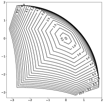
(a) $t=0.8$

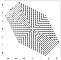
(b) $t=1.0$

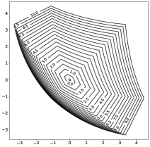
(c) $t=1.1$

Figure 1: $B^{r}_{\tilde{V}^{d}_{t}}$ balls of $\|\cdot\|_{\text{\tiny$t$-NH}}$ distance of different radii ($r\leq 10$) on $\tilde{V}^{3}_{t}$ shown along the first two dimensions.

Tempered Exponential Measures

TEMs (Amid et al., 2023b) are defined as a generalization of the exponential family with unnormalized densities. TEMs admit the following canonical form

$$\begin{split}\tilde{p}_{t|\bm{\theta}}(\bm{x})&=\frac{\exp_{t}\big{(}\bm{\theta}\cdot\bm{\varphi}(\bm{x})\big{)}}{\exp_{t}(G_{t}(\bm{\theta}))}=\exp_{t}\big{(}\bm{\theta}\cdot\bm{\varphi}(\bm{x})\ominus_{t}G_{t}(\bm{\theta})\big{)}\,,\end{split}$$ (6)

where $\bm{\theta}$ is the natural parameters, $\bm{\varphi}(\bm{x})$ is the sufficient statistics, and $G_{t}(\bm{\theta})$ is the cumulant function. The exponential family of distributions is a special form when $t=1$. However, TEMs impose the unit mass constraint (ensured by the cumulant function) not on the measure itself but on a relevant quantity called the co-density, $p_{t|\bm{\theta}}=\tilde{p}^{1/t^{*}}_{t|\bm{\theta}}$, that is, $\int p_{t|\bm{\theta}}(\bm{x})\mathrm{d}\xi=\int\tilde{p}^{1/t^{*}}_{t|\bm{\theta}}(\bm{x})\mathrm{d}\xi=1$ for $t^{*}=\frac{1}{2-t}$.

Remarkably, any discrete probability distribution $\bm{p}\in\Delta^{d}$, in which $\Delta^{d}=\{\bm{p}\in\mathbb{R}_{+}^{d}|\sum_{i}p_{i}=1\}$ denotes the $(d-1)$-dimensional probability simplex, can be characterized uniquely via a discrete TEM, i.e., $\tilde{\bm{p}}\in\tilde{\Delta}_{t}^{d}$ in the co-simplex $\tilde{\Delta}_{t}^{d}=\{\tilde{\bm{p}}\in\mathbb{R}_{+}^{d}|\sum_{i}\tilde{p}^{1/t^{*}}_{i}=1\}$ via the transformation $\tilde{\bm{p}}=\bm{p}^{t^{*}}$. Note that for $t=1$, we have $\tilde{\Delta}_{1}^{d}=\Delta^{d}$ and the identification is trivial. In this paper, we focus on different parameterizations of discrete TEMs induced by a closely related concept, the negative tempered entropy function, which in the discrete case can be written as

$$F_{t}(\tilde{\bm{p}})=\sum_{i\in[d]}\big{(}\tilde{p}_{i}\log_{t}\tilde{p}_{i}-\log_{t-1}\tilde{p}_{i}\big{)}\,.$$ (7)

TEMs are motivated by maximizing the tempered relative entropy subject to a moment constraint (and unit mass of the corresponding co-density). For $t=1$, (7) reduces to the negative Shannon entropy function (extended to positive measures), and thus, we recover the exponential family formulation.

2.2 Parameterizations of Discrete TEMs

We first discuss a parameterization for discrete TEMs based on the dual of the negative tempered entropy function (7) in the reduced form. This parameterization is a generalization of the reduction of the number of parameters for discrete distributions by one by utilizing the normalization constraint. Next, we consider the overparameterized form where the parameterizations are attained via the unconstrained and constrained Legendre dual of (7).

Minimal Form

The family $\tilde{\bm{p}}\in\tilde{\Delta}_{t}^{d}$ of discrete TEMs can be written in the canonical form (6) by taking an arbitrary nonzero component, e.g., $\tilde{p}_{d}$, where $\tilde{p}_{d}=\big{(}1-\sum_{i\in[d-1]}\tilde{p}_{i}^{1/{t^{*}}}\big{)}^{t^{*}}$ and defining the natural parameters $\hat{\theta}_{i}=\log_{t}\frac{\tilde{p}_{i}}{\tilde{p}_{d}}$ and $G_{t}(\hat{\bm{\theta}})=\log_{t}\frac{1}{\tilde{p}_{d}}$. We can then write

$$\tilde{p}(x)=\frac{\exp_{t}(\sum_{i\in[d-1]}\hat{\theta}_{i}\delta_{i}(x))}{\exp_{t}(G_{t}(\hat{\bm{\theta}}))}\,,$$

where $\delta_{i}(x)=1$ if $x=i$ and $0$ otherwise. The negative of the tempered entropy function and the corresponding derivative (also called the link) function for this case is given by

$$\hat{F}_{t}(\tilde{\bm{p}}) =\sum_{i\in[d]}\tilde{p}_{i}\log_{t}\tilde{p}_{i}\,,$$

$$[\hat{f}_{t}(\tilde{\bm{p}})]_{i} =\frac{\partial\hat{F}_{t}(\tilde{\bm{p}})}{\partial\tilde{p}_{i}}=\log_{t}\frac{\tilde{p}_{i}}{\tilde{p}_{d}}=\hat{\theta}_{i}\,,\,i\in[d-1]\,.$$

The Legendre dual (Hiriart-Urruty and Lemaréchal, 2001) and the inverse link are given by

$$\hat{F}^{*}_{t}(\hat{\bm{\theta}}) =\log_{t}\Big{[}\big{(}1+\sum_{i\in[d-1]}\exp_{t}^{1/{t^{*}}}\hat{\theta}_{i}\big{)}^{t^{*}}\Big{]}\,,$$

$$[\hat{f}^{*}_{t}(\hat{\bm{\theta}})]_{i} =\frac{\exp_{t}\hat{\theta}_{i}}{\big{(}1+\sum_{i\in[d-1]}\exp_{t}^{1/{t^{*}}}\hat{\theta}_{i}\big{)}^{t^{*}}}\,,\,i\in[d-1]\,.$$

Remarkably, the Bregman divergence (Bregman, 1967) induced by $\hat{F}_{t}$ can be simplified by the variable reduction into a convenient form given by

$$D_{\hat{F}_{t}}\!(\tilde{\bm{p}},\tilde{\bm{q}})\!=\!\!\!\!\!\!\!\sum_{i\in[d-1]}\!\!\!\!\!\tilde{p}_{i}\big{[}\log_{t}\frac{\tilde{p}_{i}}{\tilde{p}_{d}}-\log_{t}\frac{\tilde{q}_{i}}{\tilde{q}_{d}}\big{]}-\log_{t}\frac{1}{\tilde{p}_{d}}+\log_{t}\frac{1}{\tilde{q}_{d}}\,.$$

Representation	Parameter	Link	Inverse Link
Minimal Form	$\,\,\,\,\hat{\bm{\theta}}\in\mathbb{R}^{d-1}$	$[\hat{f}_{t}(\tilde{\bm{p}})]_{i}=\log_{t}\frac{\tilde{p}_{i}}{\tilde{p}_{d}}$	$[\hat{f}^{*}_{t}(\hat{\bm{\theta}})]_{i}=\frac{\exp_{t}\hat{\theta}_{i}}{\big{(}1+\sum_{i\in[d-1]}\exp_{t}^{1/{t^{*}}}\hat{\theta}_{i}\big{)}^{t^{*}}}$
Unconstrained Overparameterized	$\,\,\,\,\bm{\theta}\in\mathbb{R}^{d}$	$f_{t}(\tilde{\bm{p}})=\log_{t}\tilde{\bm{p}}$	$f^{*}_{t}(\bm{\theta})=\exp_{t}\bm{\theta}$
Constrained Overparameterized	$\,\,\,\,\check{\bm{\theta}}\in\mathbb{R}^{d}$	$\check{f}_{t}(\tilde{\bm{p}})=\log_{t}\frac{\tilde{\bm{p}}}{\tilde{\lambda}_{t}(\tilde{\bm{p}})}$	$[\check{f}^{*}_{t}(\check{\bm{\theta}})]_{i}=\frac{\exp_{t}\check{\theta}_{i}}{\big{(}\sum_{i}\exp_{t}^{1/{t^{*}}}\check{\theta}_{i}\big{)}^{t^{*}}}$

Table 1: Different parameterizations of discrete TEMs $\tilde{\bm{p}}\in\tilde{\Delta}_{t}^{d}$ via Legendre functions of the negative tempered entropy function (7).

Overparameterized Form

We start by characterizing the (unconstrained) Legendre dual of the tempered entropy function

$$\begin{split}F_{t}^{*}(\bm{\theta})\!=\!\sup_{\tilde{\bm{p}}\,\in\mathbb{R}^{d}_{+}}\!\!\big{\{}\bm{\theta}\cdot\tilde{\bm{p}}-F_{t}(\tilde{\bm{p}})\big{\}}=t^{*}\big{(}\!\!\sum_{i\in[d]}\!\!\exp_{t}^{1/t^{*}}\!\!\theta_{i}-1\big{)}\,,\end{split}$$

with the associated link $f^{*}_{t}(\bm{\theta})=\exp_{t}\bm{\theta}$. Thus, we can characterize discrete TEMs with the dual variable $\bm{\theta}=\log_{t}\tilde{\bm{p}}$ as the natural parameters and the sufficient statistics $\varphi(x)_{i}=\delta_{i}(x)\,,\,\,i\in[d]$. In this case, we have $G(\bm{\theta})=1$. The constrained dual function, on the other hand, is calculated with the additional constraint that the input argument belongs to TEMs. This characterization allows an alternative representation in an overparameterized form. The constrained Legendre dual function is defined by imposing the additional constraint that $\tilde{\bm{p}}\,\in\tilde{\Delta}_{t}^{d}$,

$$\begin{split}&\check{F}_{t}^{*}(\check{\bm{\theta}})=\sup_{\tilde{\bm{p}}\,\in\tilde{\Delta}_{t}^{d}}\big{\{}\check{\bm{\theta}}\cdot\tilde{\bm{p}}-F_{t}(\tilde{\bm{p}})\big{\}}\\ &=\sup_{\tilde{\bm{p}}\,\in\mathbb{R}^{d}_{+}}\big{\{}\check{\bm{\theta}}\cdot\tilde{\bm{p}}-F_{t}(\tilde{\bm{p}})+\lambda_{t}\,(\sum_{i\in[d]}\bm{p}_{i}^{1/{t^{*}}}-1)\,\big{\}},\end{split}$$ (8)

in which the Lagrange multiplier $\lambda_{t}$ is used to enforce the equality constraint. This yields the following duality result,

$$\check{\bm{\theta}}=\log_{t}\tilde{\bm{p}}+\lambda_{t}(\tilde{\bm{p}})\,\tilde{\bm{p}}^{1-t}=\log_{t}\frac{\tilde{\bm{p}}}{\tilde{\lambda}_{t}(\tilde{\bm{p}})}\,,$$ (9)

where $\tilde{\lambda}_{t}=1/\exp_{t}(\lambda_{t})$. In fact, $\lambda_{t}$ can be written in a closed form using an extension of the results in Amid (2020) for dual of a convex function with an equality constraint. The equality constraint $\sum_{i}\tilde{p}_{i}^{1/{t^{*}}}=1$ induces the tangent space $T_{\tilde{\bm{p}}}\tilde{\Delta}_{t}^{d}=\{\bm{u}:\tilde{\bm{p}}^{1-t}\cdot\bm{u}=0\}$ and the constrained dual variable $\check{\bm{\theta}}$ lies on this tangent space

$$\mathbf{P}_{t}(\tilde{\bm{p}})=\mathbf{I}-\frac{1}{\sum_{i}\tilde{p}_{i}^{2-2t}}\,\tilde{\bm{p}}^{1-t}\,(\tilde{\bm{p}}^{1-t})^{\top},\,\text{ and }\,\,\mathbf{P}_{t}\,\check{\bm{\theta}}=\check{\bm{\theta}}\,.$$

Proposition 1.

The Lagrange multiplier $\lambda_{t}$ for the overparameterized case can be written as

$$\lambda_{t}(\bm{\tilde{p}})=\log_{t}\Big{[}\Big{(}\frac{\sum_{i}\tilde{p}^{1-t}_{i}}{\sum_{i}\tilde{p}^{2-2t}_{i}}\Big{)}^{\frac{1}{1-t}}\Big{]}\,.$$ (10)

Remark 1.

Applying the L’Hopital’s rule to the limit case $t=1$ results in $\log$-inverse geometric mean,

$$\lambda_{1}(\bm{p})=\log\Big{(}\big{(}\prod_{i}p_{i}\big{)}^{-\frac{1}{d}}\Big{)}\,,$$

and thus yields the following parameterization for the probability vectors $\bm{p}\in\Delta^{d}$:

$$\check{\bm{\theta}}=\log\bm{p}-\frac{1}{d}\sum_{i}\log p_{i}\,\bm{1}=\log\frac{\bm{p}}{\big{(}\prod_{i}p_{i}\big{)}^{\frac{1}{d}}}\,.$$

Using Eq. (9), we can write the constrained dual convex function and the corresponding link as

$$\check{F}^{*}(\check{\bm{\theta}}) =\log_{t}\Big{[}\big{(}\sum_{i}\exp_{t}^{1/{t^{*}}}\check{\theta}_{i}\big{)}^{t^{*}}\Big{]}\,,$$ (11)

$$[\check{f}^{*}_{t}(\check{\bm{\theta}})]_{i} =\frac{\partial\check{F}^{*}_{t}(\check{\bm{\theta}})}{\partial\check{\theta}_{i}}=\frac{\exp_{t}\check{\theta}_{i}}{\big{(}\sum_{i}\exp_{t}^{1/{t^{*}}}\check{\theta}_{i}\big{)}^{t^{*}}}\,.$$ (12)

Eq. (11) introduces a tempered variant of the log-sum-exp function along with its tempered softmax link in (12). The following result is an extension of the invariance of the standard softmax along constant vectors.

Proposition 2.

The tempered softmax is invariant along the normal vector to the tangent space $\hat{\bm{n}}\,\propto\,\tilde{\bm{p}}^{1-t}$, i.e., $\check{f}^{*}(\check{\bm{\theta}}+r\,\hat{\bm{n}})=\check{f}^{*}(\check{\bm{\theta}})$ for $r\in\mathbb{R}$.

Figure 2 illustrates the relation between the constrained $\check{\bm{\theta}}$ and unconstrained $\bm{\theta}=\log_{t}\tilde{\bm{p}}$ parameterizations in the overparameterized form. Table 1 summarizes minimal and overparameterized representations.

Figure 2: Different representations for $t<1$. TEMs reside on a curved tempered co-simplex in 2D (top). The $t$-Hilbert distance is projective, thus invariant along the rays $\mathbb{R}_{+}\tilde{\Delta}_{t}^{d}$. The mapping to the unconstrained overparameterized representation is governed via the $\log_{t}$ function (left), and the corresponding variation $t$-norm distance is invariant with respect to $t$-addition of any constant $>-\frac{1}{1-t}$. The constrained overparameterized representation (right) is a $\mathbf{P}_{t}$ projection of the unconstrained form, and is mapped to the arched shaped surface $\tilde{V}_{t}^{d}$ (curved inward for $t<1$ and outward for $t>1$). At $t=1$, $\tilde{V}_{1}^{d}$ corresponds to the subspace $\{(x,y)\in\mathbb{R}^{2}\,|\,y=-x\}$ for standard exponential family.

3 Tempered Co-simplex Geometry

We lift the embeddings of the discrete probability distributions in the Hilbert simplex geometry to the embeddings of TEMs. The construction involves extending Hilbert’s projective metric to a tempered generalization. This tempered generalization is derived from first principles using, at the core, a generalized notion of Riemann sum, provided in Section 3.2.

3.1 Tempered Funk and Hilbert Distances

Consider an open bounded convex set $\Omega$. We first consider a tempered generalization of the Funk distance ($t$-Funk distance, for short) between two points $\bm{r},\bm{s}\in\Omega$:

$$\rho_{\text{\tiny$t$-FD}}^{\Omega}(\bm{r},\bm{s})=\begin{cases}\log_{t}\frac{\|\bm{r}-\bar{\bm{s}}\|}{\|\bm{s}-\bar{\bm{s}}\|}&\bm{r}\neq\bm{s}\\ 0&\bm{r}=\bm{s}\end{cases}\,.$$ (13)

Here, $\bar{\bm{s}}$ denotes the intersection of the affine ray $R(\bm{r},\bm{s})$ originating from $\bm{r}$ and passing through $\bm{s}$ with the domain boundary $\partial\Omega$. Evidently, the tempered Funk distance is also an asymmetric dissimilarity measure $\rho_{\text{\tiny$t$-FD}}^{\Omega}(\bm{r},\bm{s})\neq\rho_{\text{\tiny$t$-FD}}^{\Omega}(\bm{s},\bm{r})$ but satisfies the triangular inequality for certain cases (see Proposition 4 below). We provide a motivation for deriving the $t$-Funk distance from a tautological Finsler structure by replacing the integration for calculating the length of curves with a notion of $t$-integration in the appendix.

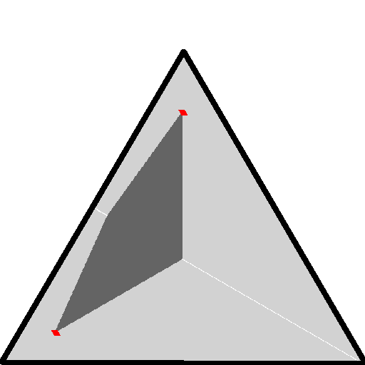
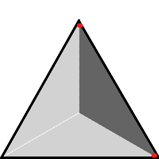
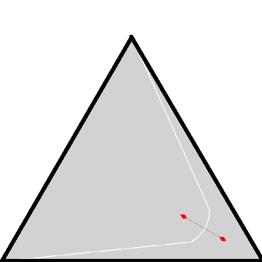
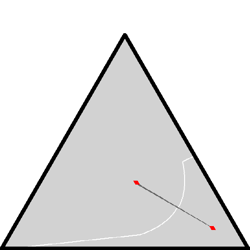
Figure 3: Voronoi bisectors (white) and triangle equality regions (dark gray) between points $p$ and $q$ with respect to Hilbert simplex distance for (from left to right) (a) $\bm{p}=(0.1,0.8,0.1)$ and $\bm{q}=(0.8,0.1,0.1)$, (b) $\bm{p}=(\varepsilon,\varepsilon,1-2\varepsilon)$ and $\bm{q}=(\varepsilon,1-2\varepsilon,\varepsilon)$, (c) $\bm{p}=(0.1,0.1,0.8)$ and $\bm{q}=(0.2,0.2,0.6)$ and (d) $\bm{p}=(0.1,0.1,0.8)$ and $\bm{q}=(0.3,0.31,0.39)$.

As the standard Hilbert distance can be viewed as a symmetrization of Funk distance, we define the tempered Hilbert distance (or $t$-Hilbert distance) between $\bm{r},\bm{s}\in\Omega$ similarly but as a $t$-symmetrization of the Funk distance:

$$\begin{split}\rho_{\text{\tiny$t$-HG}}^{\Omega}(\bm{r},\bm{s})&=\rho_{\text{\tiny$t$-FD}}^{\Omega}(\bm{r},\bm{s})\oplus_{t}\rho_{\text{\tiny$t$-FD}}^{\Omega}(\bm{s},\bm{r})\\ &=\begin{cases}\log_{t}\frac{\|\bm{r}-\bar{\bm{s}}\|\|\bm{s}-\bar{\bm{r}}\|}{\|\bm{r}-\bar{\bm{r}}\|\|\bm{s}-\bar{\bm{s}}\|}&\bm{r}\neq\bm{s}\\ 0&\bm{r}=\bm{s}\end{cases}\,,\end{split}$$ (14)

where $\bar{\bm{r}}\in\partial\Omega$ is the boundary point defined similarly as above. Indeed, $t$-Hilbert distance is independent of the underlying norm of the cross-ratio because all 1d norms are positive scalars of the absolute value. Thus, $t$-Hilbert distance only depends on the $1$-D interval domain $\Omega_{\bm{r}\bm{s}}=\Omega\cap(\bm{r}\bm{s})$. Note that we have

$$\rho_{\text{\tiny$t$-HG}}^{\Omega}(\bm{r},\bm{s})=\log_{t}\exp\rho_{1-\mathrm{HG}}^{\Omega}(\bm{r},\bm{s}).$$ (15)

Since $\log_{t}$ is a strictly monotone function, we deduced that all $t$-Hilbert Voronoi diagrams coincide.

$$\bm{\gamma}_{t}^{\Omega}(\bm{r},\bm{s})=\{\bm{t}\in\Omega:\rho_{\text{\tiny$t$-HG}}^{\Omega}(\bm{r},\bm{t})\oplus_{t}\rho_{\text{\tiny$t$-HG}}^{\Omega}(\bm{t},\bm{s})=\rho_{\text{\tiny$t$-HG}}^{\Omega}(\bm{r},\bm{s})\}\,$$

denotes a $t$-geodesics. Notably, geodesics in $t$-Hilbert geometry are no longer straight (Euclidean) lines, but rather $t$-geodesics, for all $\bm{t}\in[\bm{r}\bm{s}]$ where $[\bm{r}\bm{s}]$ is the closed line segment connecting $\bm{r}$ and $\bm{s}$. Theorem 1 extends the contraction of the $t$-Hilbert distance for positive linear maps beyond $t=1$.

Proposition 3.

The $t$-Hilbert distance $\rho_{t}^{\Omega}(p,q)$ is a metric distance for $t\geq 1$.

Theorem 1.

Let $\mathcal{C}$ be a closed pointed cone in $\mathbb{R}^{d}$. Then every positive linear map $A$ is a contraction with respect to $\rho_{\text{\tiny$t$-HG}}^{\mathcal{C}}$. Additionally, $\kappa_{\text{\tiny$t$-HG}}(A)\geq\kappa_{\mathrm{HG}}(A)$ where $\kappa_{\text{\tiny$t$-HG}}(A)$ and $\kappa_{\mathrm{HG}}(A)$ are the contraction ratios with respect to $\rho_{\text{\tiny$t$-HG}}^{\mathcal{C}}$ and $\rho_{\mathrm{HG}}^{\mathcal{C}}$, respectively.

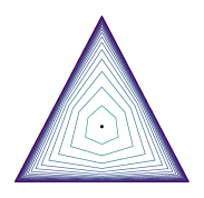
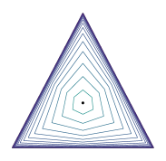
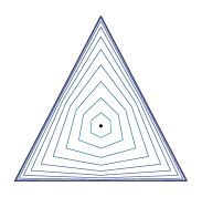
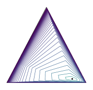
() $t=0.6$

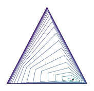
() $t=1.0$

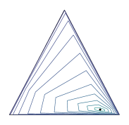
() $t=1.2$

Figure 4: Balls of different radii with respect to the $t$-Hilbert distance shown on the simplex for different $t$. The center is shown with a black dot. Darker colors indicate larger distances.

3.2 $t$-Funk and $t$-Hilbert Distances from First Principles

All the material developed in Section 3.1 follows naturally from a single change in the path that derives them from a tautological Finsler structure (Papadopoulos and Troyanov, 2014), namely the classical notion of Riemann sums. In our case, we define Riemann $t$-sums using $t$-summations ($\oplus_{t}$) instead of $+$. At the core lies the use of the $t$-addition, $\oplus_{t}$ to define Riemann $t$-sums. For any $f$ defined over a closed interval $[a,b]$ and a division $\Delta$ of this interval using $n+1$ reals $x_{0}\stackrel{{\scriptstyle\mathrm{.}}}{{=}}a<x_{1}<...<x_{n-1}<x_{n}\stackrel{{\scriptstyle\mathrm{.}}}{{=}}b$, we let

$$S_{\Delta}(f) \stackrel{{\scriptstyle\mathrm{.}}}{{=}} (\mbox{\Large$\oplus$}_{t})_{i=1}^{n}(x_{i}-x_{i-1})f(\xi_{i})$$

define the Riemann $t$-sum of $f$ over $[a,b]$ using $\Delta$, with $\xi_{i}\in]x_{i-1},x_{i}[,\forall i$. As $n$ increases, we see that the terms factoring monomials in $(1-t)$ of degree $i$ become akin to general volumes in dimension $i+1$: for $i=0$, we get ordinary unit lengths (what Riemann sums integrate), for $i=1$, we get unit surfaces, and so on. Passing to the limit, we get a notion of $t$-integration, noted $\sideset{{}^{(t)}}{}{\int_{.}^{.}}$ (for $t=1$, this is just $\int_{.}^{.}$), which we use to define the $t$-length of a curve. The $t$-Funk distance is then induced via the $t$-length of a ray connecting two points in a tautological Finsler structure. Because the construction is lengthy, details are provided in Appendix B.

3.3 $t$-Hilbert Co-simplex Distance

The co-simplex $\tilde{\Delta}_{t}^{d}$ is non-convex for $t\neq 1$, and naturally, we cannot define tempered Funk and Hilbert distance to this set. However, we can apply these distances directly on the simplex by lifting each pair of TEMs $\tilde{\bm{p}},\tilde{\bm{q}}\in\tilde{\Delta}_{t}^{d}$ to its corresponding co-density $\bm{p},\bm{q}\in\Delta^{d}$ via the following lemma.

Lemma 1.

$$t^{*}\rho^{\Delta^{d}}_{\text{\tiny$t^{*}$-FD}}(\tilde{\bm{p}}^{1/t^{*}}\!\!,\tilde{\bm{q}}^{1/t^{*}})=\log_{t}\max_{i}\frac{\tilde{p}_{i}}{\tilde{q}_{i}}\,.$$

We thus define the tempered Funk distance on the co-simplex as $\rho_{\text{\tiny$t$-FD}}(\tilde{\bm{p}},\tilde{\bm{q}})=t^{*}\rho^{\Delta^{d}}_{\text{\tiny$t^{*}$-FD}}(\tilde{\bm{p}}^{1/t^{*}}\!\!,\tilde{\bm{q}}^{1/t^{*}})$ and consequently, the tempered Hilbert on the co-simplex as its $t$-symmetrization:

$$\begin{split}\rho_{\text{\tiny$t$-HG}}(\tilde{\bm{p}},\tilde{\bm{q}})&=\rho_{\text{\tiny$t$-FD}}(\tilde{\bm{p}},\tilde{\bm{q}})\oplus_{t}\rho_{\text{\tiny$t$-FD}}(\tilde{\bm{q}},\tilde{\bm{p}})=\log_{t}\max_{i}\frac{\tilde{p}_{i}}{\tilde{q}_{i}}\max_{i}\frac{\tilde{q}_{i}}{\tilde{p}_{i}}=\log_{t}\frac{\max_{i}\frac{\tilde{p}_{i}}{\tilde{q}_{i}}}{\min_{i}\frac{\tilde{p}_{i}}{\tilde{q}_{i}}}\,.\end{split}$$ (16)

Figure 3 illustrates the Voronoi bisector $\mathrm{Bi}(\bm{p},\bm{q})=\{\bm{x}\in\Delta^{d}{\ :\ }\rho_{\mathrm{HG}}(\bm{p},\bm{x})=\rho_{\mathrm{HG}}(\bm{q},\bm{x})\}$ (studied in (Shao and Nielsen, 2017; Gezalyan and Mount, 2023)) and the triangle equality region $R(\bm{p},\bm{q})=\{\bm{x}\in\Delta^{d}{\ :\ }\rho_{\mathrm{HG}}(\bm{p},\bm{x})+\rho_{\mathrm{HG}}(\bm{x},\bm{q})=\rho_{\mathrm{HG}}(\bm{p},\bm{q})\}$ ($(d-1)$-dimensional counterpart of a geodesic) for a pair of points $\bm{p}$ and $\bm{q}$ (red) with respect to the Hilbert simplex distance. Observe that when $\bm{p}$ and $\bm{q}$ are collinear with a simplex vertex (Figure 3 (c)), $R(\bm{p},\bm{q})$ is 1D. The Voronoi bisectors are identical for the $t$-Hilbert co-simplex distance as the distance is monotonic with respect to the Hilbert simplex distance (see Theorem 1). However, the triangle equality regions correspond to $t$-triangle equality where $+$ is replaced with $\oplus_{t}$.

The following proposition summarizes the properties of the $t$-Hilbert distance.

Proposition 4.

$\rho_{\text{\tiny$t$-HG}}$ satisfies the following properties:

• (projective distance) $\rho_{\text{\tiny$t$-HG}}(\tilde{\bm{p}},\tilde{\bm{q}})=0$ iff $\tilde{\bm{p}}=K\cdot\tilde{\bm{q}}$ for some $K>0$.

• (symmetry) $\rho_{\text{\tiny$t$-HG}}(\tilde{\bm{p}},\tilde{\bm{q}})=\rho_{\text{\tiny$t$-HG}}(\tilde{\bm{q}},\tilde{\bm{p}})$.

• (triangle inequality) $\rho_{\text{\tiny$t$-HG}}(\tilde{\bm{p}},\tilde{\bm{r}})\leq\rho_{\text{\tiny$t$-HG}}(\tilde{\bm{p}},\tilde{\bm{q}})+\rho_{\text{\tiny$t$-HG}}(\tilde{\bm{q}},\tilde{\bm{r}})$ for $1\leq t<2$.

• ($t$-triangle inequality) $\rho_{\text{\tiny$t$-HG}}(\tilde{\bm{p}},\tilde{\bm{r}})\leq\rho_{\text{\tiny$t$-HG}}(\tilde{\bm{p}},\tilde{\bm{q}})\oplus_{t}\rho_{\text{\tiny$t$-HG}}(\tilde{\bm{q}},\tilde{\bm{r}})$ for $t\in\mathbb{R}$.

In addition, the $t$-Hilbert distance satisfies a notion of information monotonicity for any coarse-graining of the input arguments. However, the reduction needs to be performed on the corresponding co-densities, as outlined in the following lemma.

Lemma 2 (Monotonicity).

Let $\tilde{\bm{p}},\tilde{\bm{q}}\in\Delta^{m}_{t}$. Let $\tilde{\bm{p}}_{r}=((\tilde{p}_{1}^{1/{t^{*}}}+\tilde{p}_{2}^{1/{t^{*}}})^{t^{*}},\cdots,\tilde{p}_{d})$ and $\tilde{\bm{q}}_{r}=((\tilde{q}_{1}^{1/{t^{*}}}+\tilde{q}_{2}^{1/{t^{*}}})^{t^{*}},\cdots,\tilde{q}_{d})$ denote their coarse-grained points on $\tilde{\Delta}^{d}_{t}$. We have

$$\rho_{\text{\tiny$t$-FD}}(\tilde{\bm{p}}_{r},\tilde{\bm{q}}_{r})\leq\rho_{\text{\tiny$t$-FD}}(\tilde{\bm{p}},\tilde{\bm{q}})\,.$$

We can extend Lemma 2 to any partitioning $\mathcal{X}=\{X_{1},\ldots,X_{m}\}$ of $\{1,\ldots,d\}$ where $m\leq d$ such that $\tilde{p}_{|\mathcal{X}}[i]=(\sum_{j\in X_{i}}\tilde{p}_{j}^{1/t^{*}})^{t^{*}}$. We say the distance $D$ is $t$-information monotone if $D(\tilde{\bm{p}}_{|\mathcal{X}},\tilde{\bm{q}}_{|\mathcal{X}})\leq D(\tilde{\bm{p}},\tilde{\bm{q}})$.

Theorem 2.

The tempered Funk distance $\rho_{\text{\tiny$t$-FD}}$ and the tempered Hilbert distance $\rho_{\text{\tiny$t$-HG}}$ in $\tilde{\Delta}_{t}^{d}$ satisfy the $t$-information monotonicity.

The proof follows by iteratively applying Lemma 2 and using the definition of the tempered Hilbert distance (16).

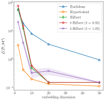
(a) $100$ random points in $\mathbb{R}^{500}$

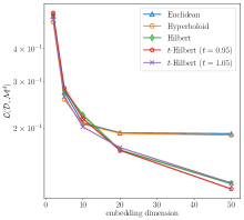
(b) Erdös-Rényi graphs ($n=200$, $p=0.5$)

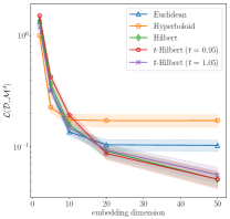
(c) Barabaási-Albert graphs ($n=200$, $m=2$)

Figure 5: Embedding loss across different embedding dimensions on three datasets.

3.4 Non-linear Embeddings of TEMs

We show an isometry of the co-simplex of TEMs to a surface with a corresponding distance $(\tilde{V}^{d}_{t},\|\cdot\|_{\text{\tiny$t$-NH}})$. Let $\tilde{V}^{d}_{t}=\{\bm{v}\in\mathbb{R}^{d}\,|\,\bm{v}\cdot\check{f}^{*}(\bm{v})^{1-t}=0\}$ be the surface of $d$-dimensional vectors that are orthogonal to the normal of the co-simplex at the corresponding TEM  given by the tempered softmax link (12). This surface is the generalization of the linear vector space defined for the Hilbert simplex geometry at $t=1$. We define the distance $\|\cdot\|_{\text{\tiny$t$-NH}}$ in $\tilde{V}^{d}_{t}$ by first introducing the ball of radius $r$ as

$$B^{r}_{\tilde{V}^{d}_{t}}=\{\bm{u}\in\mathbb{R}^{d}:|u_{i}\ominus_{t}u_{j}|\leq r,\forall i\neq j\}\,.$$ (17)

The distance between $\bm{v},\bm{v}^{\prime}\in\tilde{V}^{d}_{t}$ is then defined as

$$\begin{split}\rho_{\text{\tiny$t$-NH}}(\bm{v},\bm{v}^{\prime})&=\|\bm{v}\ominus_{t}\bm{v}^{\prime}\|_{\text{\tiny$t$-NH}}=\inf\{\tau:\,\bm{v}\ominus_{t}\bm{v}^{\prime}\in B^{\tau}_{\tilde{V}^{d}_{t}}\}\,.\end{split}$$ (18)

We can now establish our first isometry result for discrete TEMs.

Theorem 3.

The space of discrete TEMs with the $t$-Hilbert distance $(\tilde{\Delta}_{t}^{d},\rho_{\text{\tiny$t$-HG}})$ is isometric to $(\tilde{V}^{d}_{t},\rho_{\text{\tiny$t$-NH}})$ via the constrained overparameterized representation (9).

Next, we introduce an extension of the variation semi-norm, defined in Nielsen and Sun (2023). Let

$$\|\bm{x}\|_{\text{\tiny$t$-var}}=\max_{i}x_{i}\ominus_{t}\min_{i}x_{i}\,.$$ (19)

The function $\|\cdot\|_{\text{\tiny$t$-var}}$ is positive definite and satisfies $t$-triangle inequality, but does not satisfy absolute homogeneity. Moreover, similar to its $t=1$ base case, $\|r\,\bm{1}\|_{\text{\tiny$t$-var}}=0$ for any $r\in\mathbb{R}$ (see the appendix). Our second result establishes an isometry for the discrete TEMs to $\mathbb{R}^{d}$ via the semi-norm $\|\cdot\|_{\text{\tiny$t$-var}}$.

Theorem 4.

The space of discrete TEMs with the $t$-Hilbert distance $(\tilde{\Delta}_{t}^{d},\rho_{\text{\tiny$t$-HG}})$ is isometric to $(\mathbb{R}^{d},\rho_{\text{\tiny$t$-var}})$ via the unconstrained overparameterized representation mapping given by $\bm{\theta}=\log_{t}\tilde{\bm{p}}\in\mathbb{R}^{d}$ where

$$\rho_{\text{\tiny$t$-var}}(\bm{\theta},\bm{\theta}^{\prime})=\|\bm{\theta}\ominus_{t}\bm{\theta}^{\prime}\|_{\text{\tiny$t$-var}}\,.$$ (20)

Remark 2.

In fact, we have

$$\rho_{\text{\tiny$t$-var}}(\bm{\theta},\bm{\theta}^{\prime})=\rho_{\text{\tiny$t$-var}}(\check{\bm{\theta}},\check{\bm{\theta}}^{\prime})=\rho_{\text{\tiny$t$-NH}}(\bm{\theta},\bm{\theta}^{\prime})\,,$$

and the two distances are interchangeable for the construction.

3.5 Differentiable Approximations

The $\max$ operator in the $t$-Funk and $t$-Hilbert distance is non-differentiable. Similar to Nielsen and Sun (2023), we explore differentiable approximations of the distances via smoothening the $\max$ function. Our approximation is based on the tempered log-sum-exp function

$$\text{LSE}_{t}(\bm{x},T)=\frac{1}{T}\,\log_{t}\sum_{i}\exp_{t}(Tx_{i})\,,$$ (21)

using which we define the differentiable $t$-Funk and $t$-Hilbert distance with smoothing factor $T$ via the $\text{LSE}_{t}$ approximation by setting $x_{i}=\log_{t}\frac{\tilde{p}_{i}}{\tilde{q}_{i}}$ as

$$\rho_{\text{\tiny$t$-dFD}}(\tilde{\bm{p}},\tilde{\bm{q}},T) =\text{LSE}_{t}(\log_{t}\frac{\tilde{\bm{p}}}{\tilde{\bm{q}}},T)\,,$$

$$\rho_{\text{\tiny$t$-dHG}}(\tilde{\bm{p}},\tilde{\bm{q}},T) =\rho_{\text{\tiny$t$-dFD}}(\tilde{\bm{p}},\tilde{\bm{q}},T)\oplus_{t}\rho_{\text{\tiny$t$-dFD}}(\tilde{\bm{q}},\tilde{\bm{p}},T)\,.$$

We delegate the approximation error of the differentiable approximation as well as further experimental analysis to the appendix. The balls of various radii with respect to $\rho_{\text{\tiny$t$-dHG}}$ for different smoothing factors $T$ are shown in Figure 7.

3.6 Comparing Different Geometries

We compare the representation quality of different geometries for embedding a set of points from three different datasets: i) randomly sampled points in $\mathbb{R}^{500}$, ii) Erdös-Rényi graphs, and iii) Barabaási-Albert graphs. The datasets are generated according to Nielsen and Sun (2023), and the details are given in the appendix. We plot the approximation loss in Figure 5. We observe that the $t$-Hilbert distance provides some advantage compared to the other geometries for slightly larger or smaller values of $t$ than one.

4 Conclusion

Discrete $t$-tempered exponential measures (TEMs) $\tilde{p}$ are positive measures obtained from maximum entropy defined according to $t$-logarithms/$t$-exponentials (Amid et al., 2023b). TEMs form a family $\tilde{\Delta}_{t}^{d}$ with normalized codensities $\tilde{p}^{2-t}$ falling inside the probability simplex $\Delta^{d}$. In this work, we first presented the minimal and overparameterized constrained/unconstrained parameterizations of discrete TEMs. We then described their embeddings using a generalization of Hilbert’s geometry with corresponding $t$-Hilbert distance satisfying the information monotonicity (Theorem 1). We elicited isometric embeddings of $t$-Hilbert TEM spaces in Theorem 2 and Theorem 3. Last, we reported a differentiable approximation of the $t$-Hilbert distances for machine learning and experimentally studied its approximation properties and embedding performance (Figure 5). Besides, this work extends the $t$-calculus (Nivanen et al., 2003) by unraveling tempered extensions of the derivative and Riemannian integration which should prove useful in other settings.

An interesting open problem is to develop matrix Funk distances, properly integrating the case when matrices have different eigensystems. This is non-trivial because intuitively (all other things being equal), the distance should be largest when the eigensystems are the same, mimicking the fact that learning is often hardest in that case (Koolen et al., 2011).

Appendix A Deformed $t$-logarithms and $t$-exponentials, and $t$-algebra

By observing that the ordinary logarithm $\log(x)$ can be expressed as the definite Riemannian integral $\log(x)=\int_{1}^{x}\frac{1}{u}\mathrm{d}u$ measuring the oriented area underneath the graph of the strictly decreasing function $f(u)=\frac{1}{u}$, one can generalize the logarithm by using any arbitrary strictly decreasing positive function $f(u)$ (Naudts, 2011): $\log_{f}(x)=\int_{1}^{x}\frac{1}{f(u)}\mathrm{d}u$ for $x>0$. Hence, we always have $\log_{f}(1)=0$. In particular, by choosing $f_{t}(u)=\frac{1}{u^{t}}$ for $t>0$, we obtain the $t$-logarithm (Naudts, 2002) $\log_{t}(x)=\frac{1}{1-t}(x^{1-t}-1)$ for $t\not=1$ and $\log_{1}(u)=\log u$ when $t=1$. The reciprocal function of the $t$-logarithm is called the $t$-deformed exponential $\exp_{t}(y)$: $\frac{1}{1-t}(x^{1-t}-1)=y\Rightarrow x=\exp_{t}(y)=(1+(1-t)y)^{\frac{1}{1-t}}$ provided that $1+(1-t)y\geq 0$. Hence, we define $\exp_{t}(y)=[(1+(1-t)y)^{\frac{1}{1-t}}]_{+}$ for $t\not=1$ where $[u]_{+}=\max(u,0)$, and $\exp_{1}(y)=\exp(y)$. Notice that clipping of the $t$-exponentials may occur depending on the value of $t$.

Appendix B Tempered Funk Distance from a Weak Finsler Structure

We review some preliminary material related to Finsler geometry. The interested reader is referred to Troyanov (2014c, a) for further details and historical remarks.

B.1 Weak Finsler Structure on a Manifold

Definition 1.

A weak Finsler structure on a smooth Manifold $M$ is a lower-semicontinuous function $F:TM\rightarrow[0,\infty]$, called the Lagrangian, such that for every point $\bm{x}\in M$ and and tangent vectors $\bm{\xi},\bm{\xi}_{1},\bm{\xi}_{2}\in T_{\bm{x}}M$ the following properties hold:

1. $F(\bm{x},\lambda\,\bm{\xi})=\lambda\,F(\bm{x},\bm{\xi})$ for all $\lambda\geq 0$

2. $F(\bm{x},\bm{\xi}_{1}+\bm{\xi}_{2})\leq F(\bm{x},\bm{\xi}_{1})+F(\bm{x},\bm{\xi}_{2})$ (triangular inequality)

In addition, if $F:TM\rightarrow[0,\infty]$ is finite and continuous and if $F(\bm{x},\lambda\,\bm{\xi})>0$ for $\bm{\xi}\neq\bm{0}$, then $F$ is called a Finsler structure.

Note that a weak Finsler structure is a weak Minkowski norm at every point $\bm{x}\in M$. For instance, a weak Finsler structure on $T_{\bm{x}}M\subseteq\mathbb{R}^{n}$ can be obtained from a weak Minkowski norm $F_{0}:\mathbb{R}^{n}\rightarrow\mathbb{R}$ by setting

$$F(\bm{x},\bm{\xi})=F_{0}(\bm{\xi})\,.$$

Given a Finsler structure $F$ on $M$, its domain $\mathcal{D}_{F}\subseteq TM$ is defined as the set of all vectors with finite $F$-norm. The unit domain $\mathcal{U}$ is defined as the bundle of all tangent unit balls,

$$\mathcal{U}=\{(\bm{x},\bm{\xi})\in TM|F(\bm{x},\bm{\xi})<1\}\,.$$

The restriction $\mathcal{U}_{\bm{x}}=\mathcal{U}\cap T_{\bm{x}}M$ is a bounded convex set. A weak Finsler structure can be recovered from its unit domain via

$$F(\bm{x},\bm{\xi})=\inf_{\tau>0}\frac{1}{\tau}\bm{\xi}\in\mathcal{U}_{\bm{x}}\,.$$

Our construction generalizes the notion of length in a Finsler geometry. Given a Finsler structure $F$ on $M$, the forward-length of a smooth curve $\bm{\gamma}:[0,1]\rightarrow M$ is defined as

$$\ell^{+}(\bm{\gamma})=\int_{0}^{1}F(\bm{\gamma}(s),\dot{\bm{\gamma}}(s))\,\mathrm{d}s\,.$$ (22)

We may also define the backward-length

$$\ell^{-}(\bm{\gamma})=\int_{0}^{1}F(\bm{\gamma}(s),-\dot{\bm{\gamma}}(s))\,\mathrm{d}s\,.$$ (23)

The forward- and backward-lengths coincide when the Minkowski norms are symmetric but differ otherwise. This explains the fact that Finsler distances are quasi-metrics that may not be necessarily symmetric (e.g., Funk) although they satisfy the triangle inequality. To contrast with oriented Finsler distances, Riemannian distances are always symmetric and hence define proper metrics (see Matveev (2012); Arnaudon and Nielsen (2012)).

To extend these definitions, we first introduce the notion of a $t$-derivative and $t$-Riemann integral. We will simply refer to the forward-length of a curve as its length and omit the $+$ superscript.

B.2 From $t$-Derivative and $t$-Riemann Integral to $t$-Length

$t$-derivative We generalize the notion of the standard derivative a scalar function $f:\mathbb{R}\rightarrow\mathbb{R}$ to a $t$-derivative.

Definition 2.

Suppose $f$ is defined on an open neighborhood of some $x\in\mathbb{R}$. When it exists, the $t$-derivative of $f$ in $x$ is the real

$$\mathrm{D}_{t}f(x)\stackrel{{\scriptstyle\mathrm{.}}}{{=}}\lim_{\delta\rightarrow 0}\frac{f(x+\delta)\ominus_{t}f(x)}{\delta}.$$ (24)

$\mathrm{D}_{t}$ generalizes the notion of standard derivative for $t=1$. Note that we can obtain a direct expression of $\mathrm{D}_{t}f$ by using the definition of $\ominus_{t}$:

$$\mathrm{D}_{t}f(x)=\lim_{\delta\rightarrow 0}\frac{1}{\delta}\cdot\frac{f(x+\delta)-f(x)}{1+(1-t)f(x)}=\frac{1}{1+(1-t)f(x)}\cdot\lim_{\delta\rightarrow 0}\frac{f(x+\delta)-f(x)}{\delta}=\frac{f^{\prime}(x)}{1+(1-t)f(x)}.$$ (25)

For instance, using (25), we can find the functions whose $t$-derivative is constant:

$$\mathrm{D}_{t}f(x)=K.$$ (26)

This involves solving a simple differential equation $f^{\prime}-(1-t)Kf=K$, whose set of solutions is easily found to be

$$f(x)=V\exp\left((1-t)Kx\right)-\frac{1}{1-t}\quad(V\mbox{ does not depend on }x).$$ (27)

Remark the difference between this function and the solution for $t=1$, which would be noted $f(x)=Kx+V$, and the risk to diverge in $t=1$. This can be prevented if we enforce the solution to converge to the solution of the conventional derivative for $t\rightarrow 1$. To get there, we compute its Taylor expansion around $t=1$,

$$f(x)=V-\frac{1}{1-t}+VKx(1-t)+\frac{VK^{2}x^{2}(1-t)^{2}}{2}+o((1-t)^{2}).$$ (28)

We see that there is only one choice, $V=1/(1-t)$, which yields the desired series, $f(x)=Kx+o(1-t)$, and we have a unique solution to the differential equation that satisfies the behavior,

$$f(x)=\frac{\exp\left((1-t)Kx\right)-1}{1-t}\quad\left(\mbox{unique solution for }\mathrm{D}_{t}f(x)=K\wedge\lim_{t\rightarrow 1}f(x)=Kx\right).$$ (29)

Proceeding in a similar way, we would find that the unique function to $\mathrm{D}_{t}\circ\mathrm{D}_{t}f(x)=K$ with $\lim_{t\rightarrow 1}f(x)=(K/2)\cdot x^{2}$ (the second order derivative of $f$ is a fixed constant, $K$) is

$$f(x)=\frac{\exp\Big{(}\frac{\frac{1}{K}\exp((1-t)\,K\,x)-(1-t)\,x-\frac{1}{K}}{1-t}\Big{)}-1}{1-t}.$$ (30)

Remark the non-trivial variations of functions in (28), (30). Using (25) or by simple calculation, we obtain

$$\mathrm{D}_{t}\log_{t}(x)\stackrel{{\scriptstyle\mathrm{.}}}{{=}}\lim_{\delta\rightarrow 0}\frac{\log_{t}(\frac{x+\delta}{x})}{\delta}=\lim_{\delta\rightarrow 0}\frac{\frac{\delta}{x}}{\delta}=\frac{1}{x}.$$ (31)

Thus, for $\delta\ll x$, we can define an expansion

$$\log_{t}(x+\delta)\approx\log_{t}(x)\oplus_{t}\frac{\delta}{x}.$$ (32)

$t$-Riemann Integral We wish to define a generalization of Riemann integration to the tempered algebra and for this objective, given an interval $[a,b]$ and a division $\Delta$ of this interval using $n+1$ reals $x_{0}\stackrel{{\scriptstyle\mathrm{.}}}{{=}}a<x_{1}<...<x_{n-1}<x_{n}\stackrel{{\scriptstyle\mathrm{.}}}{{=}}b$, we define the Riemann $t$-sum over $[a,b]$ using $\Delta$ as

$$S_{\Delta}(f) \stackrel{{\scriptstyle\mathrm{.}}}{{=}} (\mbox{\Large$\oplus$}_{t})_{i=1}^{n}|\mathbb{I}_{i}|f(\xi_{i}),\quad(\mathbb{I}_{i}\stackrel{{\scriptstyle\mathrm{.}}}{{=}}[x_{\pi(i)-1},x_{\pi(i)}],|\mathbb{I}_{i}|\stackrel{{\scriptstyle\mathrm{.}}}{{=}}x_{\pi(i)}-x_{\pi(i)-1}),\xi_{i}\in\mathbb{I}_{i},$$

where $\pi$ is any permutation of $[n]\stackrel{{\scriptstyle\mathrm{.}}}{{=}}\{1,2,...,n\}$ ($\oplus_{t}$ is commutative, so changing $\pi$ does not change the result; we do not put the $\xi_{i}$s in the argument of $S_{.}$ for readability). In the classical definition, $\pi=\mathrm{id}$. It will be useful to remember that we can fix beforehand the $\xi_{i}$s so they are given for a given division. Let $s(\Delta)\stackrel{{\scriptstyle\mathrm{.}}}{{=}}\max_{i}|\mathbb{I}_{i}|$ denote the step of division $\Delta$. The conditions for $t$-Riemann integration are the same as for $t=1$.

Definition 3.

A continuous function $f:[a,b]\rightarrow\mathbb{R}$ is $t$-Riemann integrable iff there exists $L$ such that

$$\forall\varepsilon>0,\exists\delta>0:\forall\mbox{ division }\Delta\mbox{ with }s(\Delta)<\delta,\left|S_{\Delta}(f)-L\right|<\varepsilon.$$ (33)

When this happens, we note

$$\sideset{{}^{(t)}}{}{\int_{a}^{b}}f(x)\mathrm{d}_{t}x=L.$$ (34)

$t$-Riemann Integral We define

$$\sideset{{}^{(t)}}{}{\int_{a}^{b}}f(x)\mathrm{d}_{t}x=F(b)\ominus_{t}F(a),$$ (35)

as the $t$-integral of $f$, where $F$ is called a $t$-primitive s.t. $\mathrm{D}_{t}F=f$. For instance, from (31) and for $a,b\geq 0$, we have

$$\sideset{{}^{(t)}}{}{\int_{a}^{b}}\frac{1}{x}\,\mathrm{d}_{t}x=\log_{t}b\,\ominus_{t}\,\log_{t}a=\log_{t}\frac{b}{a}\,.$$ (36)

$t$-Length We use (35) to define a generalization of length to a $t$-length for smooth curve on a Finsler manifold. Let $\bm{\gamma}:[0,1]\rightarrow M$ denote a smooth curve on a Finsler manifold with a Finsler structure $F$. We define the (forward) $t$-length of the curve $\bm{\gamma}$ as

$$\ell^{(t)}(\bm{\gamma})\stackrel{{\scriptstyle\mathrm{.}}}{{=}}\sideset{{}^{(t)}}{}{\int_{0}^{1}}F(\bm{\gamma}(s),\dot{\bm{\gamma}}(s))\,\mathrm{d}_{t}s\,.$$ (37)

B.3 Tautological Finlser Structure of a Convex Set

Definition 4.

Given a proper convex set $\Omega$, the tautological weak Finsler structure $F_{f}$ on $\Omega$ is the Finsler structure for which the unit ball at a point $\bm{x}\in\Omega$ is the domain $\Omega$ itself, with the point $\bm{x}$ as the center, thus, resulting the unit domain

$$\mathcal{U}=\{(\bm{x},\bm{\xi})\in T\Omega\,|\,\bm{\xi}\in\Omega-\bm{x}\}\,,$$ (38)

where the $\Omega-\bm{x}$ should be viewed as a translation of the convex set $\Omega$ by the point $\bm{x}$. The Lagrangian is then given by

$$F_{f}(\bm{x},\bm{\xi})=\inf\{\tau>0\,|\,\bm{x}+\frac{\bm{\xi}}{\tau}\in\Omega\}\,,$$ (39)

Consequently, $\bm{x}+\frac{\bm{\xi}}{F_{f}(\bm{x},\bm{\xi})}\in\partial\Omega$, otherwise $F_{f}(\bm{x},\bm{\xi})=0$ if the ray $\bm{x}+\mathbb{R}_{+}\bm{\xi}$ is contained in $\Omega$.

In can be shown that the tautological Finsler structure of a half-space $\mathcal{H}=\{\bm{x}\in\mathbb{R}^{d}\,|\,\bm{\nu}\cdot\bm{x}\leq c\}\in\mathbb{R}^{d}$ is given by

$$F_{f}(\bm{x},\bm{\xi})=\max\Big{(}\frac{\bm{\nu}\cdot\bm{\xi}}{c-\bm{\nu}\cdot\bm{x}},\,0\Big{)}\,.$$ (40)

Theorem 5.

The tautological distance in a proper convex domain $\Omega\in\mathbb{R}^{d}$ induced by the $t$-length of the ray is given by

$$\rho_{f}(\bm{r},\bm{s})=\log_{t}\frac{\|\bm{r}-\bar{\bm{s}}\|}{\|\bm{s}-\bar{\bm{s}}\|}\,,$$ (41)

where $\bar{\bm{s}}$ is the intersection of the ray $R(\bm{r},\bm{s})$ emanating from $\bm{r}$ and passing through $\bm{s}$ with the boundary $\partial\Omega$. If the ray is contained in $\Omega$, then $\bar{\bm{s}}$ is considered to be a point at infinity and therefore, $\rho_{f}(\bm{r},\bm{s})=0$.

Note that the tautological distance via the $t$-length in (41) is identical to the $t$-Funk distance we define in (13). To prove Theorem 5, we first need to restate two lemmas from Troyanov (2014a).

Lemma 3 (Troyanov (2014a)).

Let $\Omega_{1}$ and $\Omega_{2}$ be two convex domains in $\mathbb{R}^{d}$. If $F_{1}$ and $F_{2}$ are the corresponding tautological structures, then

$$\Omega_{1}\subseteq\Omega_{2}\Longleftrightarrow F_{1}(\bm{x},\bm{\xi})\geq F_{2}(\bm{x},\bm{\xi})$$

for all $(\bm{x},\bm{\xi})\in T\Omega_{1}$.

Lemma 4 (Troyanov (2014a)).

Let $\Omega$ be a convex domain in $\mathbb{R}^{d}$ and $\bm{r},\bm{s}\in\Omega$. If $\bm{s}=\bm{r}+\tau\bm{\xi}$ for some $\bm{\xi}\in\mathbb{R}^{d}$ and $\tau\geq 0$, then

$$F_{f}(\bm{s},\bm{\xi})=\frac{F_{f}(\bm{r},\bm{\xi})}{1-\tau\,F_{f}(\bm{r},\bm{\xi})}\,.$$ (42)

Proof of Theorem 5.

We start by calculating the distance when the domain is a half-space $\Omega=\mathcal{H}=\{\bm{x}\in\mathbb{R}^{d}\,|\,\bm{\nu}\cdot\bm{x}\leq c\}$ for some $\bm{\nu}\neq\bm{0}$ by $t$-integrating (40) along a curve $\bm{\beta}$ connecting $\bm{r}$ and $\bm{s}$:

$$\rho^{\mathcal{H}}_{f}(\bm{r},\bm{s}) =\sideset{{}^{(t)}}{}{\int_{0}^{1}}\max\Big{(}\frac{\bm{\nu}\cdot\dot{\bm{\beta}}(\tau)}{c-\bm{\nu}\cdot\bm{\beta}(\tau)},\,0\Big{)}\mathrm{d}_{t}\tau$$

$$=\sideset{{}^{(t)}}{}{\int_{0}^{1}}\max\Big{(}\frac{(c-\bm{\nu}\cdot\bm{\beta}(\tau))^{\prime}}{|c-\bm{\nu}\cdot\bm{\beta}(\tau)|},\,0\Big{)}\mathrm{d}_{t}\tau$$

$$=\max\Big{(}\log_{t}\big{(}\frac{c-\bm{\nu}\cdot\bm{r}}{c-\bm{\nu}\cdot\bm{s}}\big{)},\,0\Big{)}\,.$$ (43)

Suppose $\bm{a}\in\partial\mathcal{H}$ is the boundary point along the ray emanating from $\bm{r}$ and passing through $\bm{s}$. Then $\bm{\nu}\cdot\bm{a}=c$ and can write (43)

$$\rho_{f}^{\mathcal{H}}(\bm{r},\bm{s})=\log_{t}\frac{\|\bm{a}-\bm{r}\|}{\|\bm{a}-\bm{s}\|}\,,$$ (44)

where $\|\cdot\|$ is any arbitrary norm (e.g., $\|\cdot\|_{2}$). For a general convex domain $\Omega$, let $\bm{a}\in\partial\Omega$ be defined similarly to the previous case for the points $\bm{r}$ and $\bm{s}$. We have

$$F^{\Omega}_{f}(\bm{r},\bm{\xi})=\frac{1}{\|\bm{a}-\bm{r}\|}\,,$$ (45)

where $\bm{\xi}=\frac{\bm{s}-\bm{r}}{\|\bm{s}-\bm{r}\|}$ is the unit vector along the ray connecting $\bm{r}$ and $\bm{s}$. Using Lemma 4, we have

$$F^{\Omega}_{f}(\bm{\beta}(\tau),\dot{\bm{\beta}}(\tau))=\frac{F^{\Omega}_{f}(\bm{r},\bm{\xi})}{1-\tau\,F^{\Omega}_{f}(\bm{r},\bm{\xi})}=\frac{1}{\|\bm{a}-\bm{r}\|-\tau}$$ (46)

along the curve $\bm{\beta}(\tau)=\bm{r}+\tau\,\bm{\xi}$ and thus, we can calculate the $t$-length along $\bm{\beta}$ as

$$\rho^{\Omega}_{f}(\bm{r},\bm{s}) =\sideset{{}^{(t)}}{}{\int_{0}^{\|\bm{s}-\bm{r}\|}}\frac{1}{\|\bm{a}-\bm{r}\|-\tau}\mathrm{d}_{t}\tau$$

$$=\log_{t}\frac{1}{\|\bm{a}-\bm{r}\|-\|\bm{s}-\bm{r}\|}\ominus_{t}\log_{t}\frac{1}{\|\bm{a}-\bm{r}\|}$$

$$=\log_{t}\frac{\|\bm{a}-\bm{r}\|}{\|\bm{a}-\bm{s}\|}\,,$$ (47)

since $\bm{r}$, $\bm{s}$, and $\bm{a}$ are collinear. Thus, taking $\mathcal{H}$ to be the supporting hyperplane to $\Omega$ at $\bm{a}$, we have $\rho^{\Omega}_{f}(\bm{r},\bm{s})\leq\rho^{\mathcal{H}}_{f}(\bm{r},\bm{s})$. However, from Lemma 2, we have $\rho^{\Omega}_{f}(\bm{r},\bm{s})\geq\rho^{\mathcal{H}}_{f}(\bm{r},\bm{s})$ and thus, the result holds with equality.

∎

Proposition 5.

The unit speed linear $t$-geodesic starting at $\bm{r}\in\Omega$ in the direction of $\bm{\xi}\in T_{\bm{r}}\Omega$ is the path

$$\bm{\gamma}_{\bm{r},\bm{\xi}}(\tau)=\bm{r}+\frac{1-\exp_{t}\ominus_{t}\tau}{F_{f}(\bm{r},\bm{\xi})}\,\bm{\xi}\,.$$ (48)

Proof.

By (39), we have

$$\bar{\bm{s}}=\bm{r}+\frac{\bm{\xi}}{F_{f}(\bm{r},\bm{\xi})}\,,\text{ \,\, and therefore \,\, }\bar{\bm{s}}-\bm{\gamma}(\tau)=\frac{\exp_{t}\ominus_{t}\tau}{F_{f}(\bm{r},\bm{\xi})}\cdot\bm{\xi}\,.$$

Thus, we have

$$\rho_{f}(\bm{r},\bm{\gamma}(\tau))=\log_{t}\frac{\|\bm{r}-\bar{\bm{s}}\|}{\|\bm{\gamma}(\tau)-\bar{\bm{s}}\|}=\log_{t}\frac{1}{\exp_{t}\ominus_{t}\tau}=\tau\,.$$

∎

Appendix C Properties of the Function $\|\cdot\|_{\text{\tiny$t$-var}}$

The function $\|\cdot\|_{\text{\tiny$t$-var}}$ behaves almost like a semi-$t$-norm in the following sense:

1. $t$-Subadditivity: $\sideset{{}^{(t)}}{}{\mathop{\|}}{\bm{u}\oplus_{t}\bm{v}}\|\leq\sideset{{}^{(t)}}{}{\mathop{\|}}{\bm{u}}\|\oplus_{t}\sideset{{}^{(t)}}{}{\mathop{\|}}{\bm{v}}\|$, for all $\bm{u},\bm{v}\in\mathbb{R}^{d}$.

2. Absolute homogeneity does not hold in general but for $\alpha>0$, we have: $\sideset{{}^{(t)}}{}{\mathop{\|}}{\alpha\,\bm{u}}\|=\alpha\cdot\sideset{{}^{(t_{\alpha})}}{}{\mathop{\|}}{\bm{u}}\|$, where $t_{\alpha}=1-(1-t)\alpha$ (given that $\exp_{t}(\min_{i}\alpha\,u_{i})=\exp_{t_{\alpha}}\!(\min_{i}u_{i})\neq 0$).

3. Positive semi-definiteness: $\sideset{{}^{(t)}}{}{\mathop{\|}}{\bm{u}}\|\geq 0$, and if $\sideset{{}^{(t)}}{}{\mathop{\|}}{\bm{u}}\|=0$ then $\bm{u}=r\bm{1}$ for $r\in\mathbb{R}$.

Appendix D Proofs

Proof of Proposition 1.

The proof follows by substituting the definition of $\log_{t}$ in (9) and applying the equality $\mathbf{P}_{t}\check{\bm{\theta}}=\check{\bm{\theta}}$. ∎

Proof of Proposition 2.

By (9) and for a given $r\in\mathbb{R}$, we can write

$$\check{\bm{\theta}}+r\,\hat{\bm{n}}=\check{\bm{\theta}}+r\|\tilde{\bm{p}}^{1-t}\|_{2}\cdot\tilde{\bm{p}}^{1-t}=\log_{t}\frac{\tilde{\bm{p}}}{K}\,,$$ (49)

where $K=1/\exp_{t}(\lambda+r\|\tilde{\bm{p}}^{1-t}\|_{2})$. Applying the function $\check{f}^{*}$ to the rhs concludes the proof. ∎

Proof of Proposition 3.

Consider the function $h_{t}(u)=\log_{t}\exp(u)$ which satisfies $h_{t}(u)=0$ if and only if $u=0$ for any $t$. The function $h_{t}(u)$ is increasing for $t>1$ and $x>0$ since $h_{t}^{\prime}(u)=\frac{1-\exp((1-t)u)}{t-1}>0$, and hence $h_{t}(u)\geq 0$. Function $h_{t}(u)$ is also subadditive for $t>1$ since $h_{t}(a+b)=\log_{t}(e^{a}e^{b})=\log_{t}e^{a}+\log_{t}e^{b}+(1-t)(\log_{t}e^{a})(\log_{t}e^{b})=h_{t}(a)+h_{t}(b)-(1-t)h_{t}(a)h_{t}(b)\leq h_{t}(a)+h_{t}(b)$. Thus we have the property that $h_{t}(u)$ which is a metric transform (Doboš, 1981). It follows that $\rho_{t}^{\Omega}(p,q)$ is a metric for $t\geq 1$. ∎

Proof of Theorem 1.

Given $\bm{r},\bm{s}\in\mathcal{C}$, we have

$$\rho_{\text{\tiny$t$-HG}}^{\mathcal{C}}(\bm{r},\bm{s})=\log_{t}\exp\rho_{\mathrm{HG}}^{\mathcal{C}}(\bm{r},\bm{s})\,.$$

Since $\rho_{\mathrm{HG}}^{\mathcal{C}}$ is a contraction for positive linear maps, it suffices to show that the function $x\mapsto\log_{t}\exp x$ is monotonic for $t<2$. Monotonicity simply follows from the derivative $(\log_{t}\exp)^{\prime}(x)=\exp^{1-t}(x)>0$. From Kohlberg and Pratt (1982) (Theorem 4.1) and the fact that $\rho_{\text{\tiny$t$-HG}}^{\mathcal{C}}$ is a monotonic function of $\rho_{\mathrm{HG}}^{\mathcal{C}}$, we conclude that $\kappa_{\text{\tiny$t$-HG}}(A)\geq\kappa_{\mathrm{HG}}(A)$ for all positive $A$. ∎

Proof of Lemma 1.

$$t^{*}\rho^{\Delta^{d}}_{\text{\tiny$t^{*}$-FD}}(\tilde{\bm{p}}^{1/t^{*}},\tilde{\bm{q}}^{1/t^{*}})=t^{*}\log_{t^{*}}\max_{i}\frac{\tilde{p}^{1/t^{*}}_{i}}{\tilde{q}^{1/t^{*}}_{i}}=t^{*}\max_{i}\log_{t^{*}}\frac{\tilde{p}^{1/t^{*}}_{i}}{\tilde{q}^{1/t^{*}}_{i}}=\max_{i}\log_{t}\frac{\tilde{p}_{i}}{\tilde{q}_{i}}=\log_{t}\max_{i}\frac{\tilde{p}_{i}}{\tilde{q}_{i}}\,.$$

∎

Proof of Proposition 4.

Proof of condition (i) We remark that for any $\tilde{\bm{p}},\tilde{\bm{q}}$,

$$m_{t}(\tilde{\bm{p}},\tilde{\bm{q}})\cdot\tilde{p}_{i}\leq\tilde{q}_{i}\leq M_{t}(\tilde{\bm{p}},\tilde{\bm{q}})\cdot\tilde{p}_{i},\forall i\in[m].$$ (50)

Hence, if $\rho_{\text{\tiny$t$-HG}}(\tilde{\bm{p}},\tilde{\bm{q}})=0$ then $m_{t}(\tilde{\bm{p}},\tilde{\bm{q}})=M_{t}(\tilde{\bm{p}},\tilde{\bm{q}})=K$ and $\tilde{\bm{p}}=K\cdot\tilde{\bm{q}}$, and if $\tilde{\bm{p}}=K\cdot\tilde{\bm{q}}$ then we immediately have $\rho_{\text{\tiny$t$-HG}}(\tilde{\bm{p}},\tilde{\bm{q}})=0$.

Proof of condition (ii) It follows directly from the definition of $\ominus_{t}$ and $t$-negation that $\ominus_{t}\log_{t}a/b=\ominus_{t}(\log_{t}a\ominus_{t}\log_{t}b)=\log_{t}b\ominus_{t}\log_{t}a=\log_{t}b/a$. Thus,

$$\rho_{\text{\tiny$t$-HG}}(\tilde{\bm{p}},\tilde{\bm{q}}) =\ominus_{t}\min_{i}\big{(}\log_{t}\tilde{p}_{i}\ominus_{t}\log_{t}\tilde{q}_{i}\big{)}\ominus_{t}\ominus_{t}\max_{j}\big{(}\log_{t}\tilde{p}_{j}\ominus_{t}\log_{t}\tilde{q}_{j}\big{)}=\rho_{\text{\tiny$t$-HG}}(\tilde{\bm{q}},\tilde{\bm{p}}).$$ (51)

Proof of condition (iii) Similar to the proof of Bushell (1973) (Theorem 2.1), we have

$$\tilde{\bm{p}}\leq M(\tilde{\bm{p}},\tilde{\bm{q}})\tilde{\bm{q}}\leq M(\tilde{\bm{p}},\tilde{\bm{q}})M(\tilde{\bm{q}},\tilde{\bm{r}})\tilde{\bm{r}}$$

Thus,

$$\log_{t}M(\tilde{\bm{p}},\tilde{\bm{r}})\leq\log_{t}M(\tilde{\bm{p}},\tilde{\bm{q}})\oplus_{t}\log_{t}M(\tilde{\bm{q}},\tilde{\bm{r}})\,.$$

Similarly, we have

$$\log_{t}m(\tilde{\bm{p}},\tilde{\bm{r}})\geq\log_{t}m(\tilde{\bm{p}},\tilde{\bm{q}})\oplus_{t}\log_{t}m(\tilde{\bm{q}},\tilde{\bm{r}})\,.$$

Combining the two inequalities concludes the proof of the statement.

Proof of condition (iv) We need to show

$$\log_{t}\Big{(}\frac{M(\tilde{\bm{p}},\tilde{\bm{q}})\cdot M(\tilde{\bm{q}},\tilde{\bm{r}})}{m(\tilde{\bm{p}},\tilde{\bm{q}})\cdot m(\tilde{\bm{q}},\tilde{\bm{r}})}\Big{)}\leq\log_{t}\Big{(}\frac{M(\tilde{\bm{p}},\tilde{\bm{q}})}{m(\tilde{\bm{p}},\tilde{\bm{q}})}\Big{)}+\log_{t}\Big{(}\frac{M(\tilde{\bm{q}},\tilde{\bm{r}})}{m(\tilde{\bm{q}},\tilde{\bm{r}})}\Big{)}\,,$$

for $1\leq t<2$. The inequality amounts to showing

$$\log_{t}(a\,b)\leq\log_{t}a+\log_{t}b\,,\quad a,b\geq 1,$$

or, since $(1-t)\leq 1$, to show

$$(ab)^{\tau}+1\geq a^{\tau}+b^{\tau},\,\,\,a,b\geq 1\text{ and }\tau>0.$$

Fix $a$ and consider the function $f(x)=(ax)^{\tau}+1-a^{\tau}-x^{\tau}$. Note that $f(1)=0$ and $f^{\prime}(x)=\tau\,x^{\tau-1}(a^{\tau}-1)\geq 0$. Thus, the function is increasing for all $x>1$. ∎

Proof of Lemma 2.

Denote $\iota=\max\{\tilde{p}_{1}/\tilde{q}_{1},\tilde{p}_{2}/\tilde{q}_{2}\}$. Assuming $\tilde{q}_{1},\tilde{q}_{2}>0$, we have $\tilde{p}_{1}\leq\iota\,\tilde{q}_{1}$ and $\tilde{p}_{2}\leq\iota\,\tilde{q}_{2}$. Thus,

$$\frac{(\tilde{p}_{1}^{1/{t^{*}}}+\tilde{p}_{2}^{1/{t^{*}}})^{t^{*}}}{(\tilde{q}_{1}^{1/{t^{*}}}+\tilde{q}_{2}^{1/{t^{*}}})^{t^{*}}}\leq\frac{\iota\,(\tilde{q}_{1}^{1/{t^{*}}}+\tilde{q}_{2}^{1/{t^{*}}})^{t^{*}}}{(\tilde{q}_{1}^{1/{t^{*}}}+\tilde{q}_{2}^{1/{t^{*}}})^{t^{*}}}=\iota.$$ (52)

Hence, we have

$$\log_{t}\max\left\{\frac{(\tilde{p}_{1}^{1/{t^{*}}}+\tilde{p}_{2}^{1/{t^{*}}})^{t^{*}}}{(\tilde{q}_{1}^{1/{t^{*}}}+\tilde{q}_{2}^{1/{t^{*}}})^{t^{*}}},\ldots,\frac{\tilde{p}_{d}}{\tilde{q}_{d}}\right\}\leq\log_{t}\max_{i}\frac{\tilde{p}_{i}}{\tilde{q}_{i}}.$$ (53)

The proof is complete by the definition of the $t$-Funk distance. ∎

Proof of Theorem 3.

The mapping from $\tilde{\Delta}_{t}^{d}$ via (9) is bijective. Given $\tilde{\bm{p}},\tilde{\bm{q}}\in\tilde{\Delta}_{t}^{d}$, the distance $\rho_{\text{\tiny$t$-NH}}$ between $\check{\bm{\theta}}=\log_{t}\frac{\tilde{\bm{p}}}{\tilde{\lambda}_{t}(\tilde{\bm{p}})}$ and $\check{\bm{\theta}}^{\prime}=\log_{t}\frac{\tilde{\bm{q}}}{\tilde{\lambda}_{t}(\tilde{\bm{q}})}$ amounts to

$$\rho_{\text{\tiny$t$-NH}}(\check{\bm{\theta}},\check{\bm{\theta}}^{\prime}) =\inf_{\tau}\Big{|}\log_{t}\frac{\tilde{p}_{i}}{\tilde{\lambda}_{t}(\tilde{\bm{p}})}\ominus_{t}\log_{t}\frac{\tilde{q}_{i}}{\tilde{\lambda}_{t}(\tilde{\bm{q}})}\ominus_{t}(\log_{t}\frac{\tilde{p}_{j}}{\tilde{\lambda}_{t}(\tilde{\bm{p}})}\ominus_{t}\log_{t}\frac{\tilde{q}_{j}}{\tilde{\lambda}_{t}(\tilde{\bm{q}})})\Big{|}\in B^{\tau}_{\tilde{V}^{d}_{t}}\,,\,\,i\neq j$$

$$=\inf_{\tau}\Big{|}\log_{t}\frac{\frac{\tilde{p}_{i}}{\tilde{q}_{i}}}{\frac{\tilde{p}_{j}}{\tilde{q}_{j}}}\Big{|}\in B^{\tau}_{\tilde{V}^{d}_{t}}\,,\,\,i\neq j$$

$$=\log_{t}\frac{\max_{i}\frac{\tilde{p}_{i}}{\tilde{q}_{i}}}{\min_{j}\frac{\tilde{p}_{j}}{\tilde{q}_{j}}}$$

$$=\rho_{\text{\tiny$t$-HG}}(\tilde{\bm{p}},\tilde{\bm{q}})\,.$$

∎

Proof of Theorem 4.

The mapping from $\tilde{\Delta}_{t}^{d}$ to $\mathbb{R}^{d}$ via $\log_{t}$ is bijecttive. Given $\tilde{\bm{p}},\tilde{\bm{q}}\in\tilde{\Delta}_{t}^{d}$, the distance $\rho_{tvar}$ between $\bm{\theta}=\log_{t}\tilde{\bm{p}}$ and $\bm{\theta}^{\prime}=\log_{t}\tilde{\bm{q}}$ amounts to

$$\rho_{\text{\tiny$t$-var}}(\bm{\theta},\bm{\theta}^{\prime})=\|\bm{\theta}\ominus_{t}\bm{\theta}^{\prime}\|_{\text{\tiny$t$-var}} =\max_{i}\{\log_{t}\tilde{p}_{i}\ominus_{t}\log_{t}\tilde{q}_{i}\}\ominus_{t}\min_{j}\{\log_{t}\tilde{p}_{j}\ominus_{t}\log_{t}\tilde{q}_{j}\}$$

$$=\log_{t}\frac{\max_{i}\frac{\tilde{p}_{i}}{\tilde{q}_{i}}}{\min_{j}\frac{\tilde{p}_{j}}{\tilde{q}_{j}}}=\rho_{\text{\tiny$t$-HG}}(\tilde{\bm{p}},\tilde{\bm{q}})\,.$$

∎

Appendix E Differentiable Approximations

In the following, we provide the tempered log-sum-exp function and bound its approximation error. Let

$$\text{LSE}_{t}(\bm{x},T)=\frac{1}{T}\,\log_{t}\sum_{i}\exp_{t}(Tx_{i})\,.$$

We have

$$\frac{1}{T}\,\big{(}\max_{i}Tx_{i}\oplus_{t}\varepsilon^{\ell}_{t}(\bm{x},T)\big{)}\leq\rho_{t-diff}(\bm{x},T)\leq\frac{1}{T}\,\big{(}\max_{i}Tx_{i}\oplus_{t}\varepsilon^{r}_{t}(\bm{x},T)\big{)}\,,$$ (54)

where

$$\varepsilon_{t}^{\ell}(\bm{x},T) =\log_{t}\big{(}1+(d-1)\,\exp_{t}\ominus_{t}\|T\bm{x}\|_{\text{\tiny$t$-var}}\big{)}\,,$$

$$\varepsilon_{t}^{r}(\bm{x},T) =\log_{t}\big{(}(d-1)+\exp_{t}\ominus_{t}\|T\bm{x}\|_{\text{\tiny$t$-var}}\big{)}\,.$$

Additionally, for $t\leq 1$,

$$\lim_{T\rightarrow\infty}\text{LSE}_{t}(\bm{x},T)=\max_{i}x_{i}\,.$$ (55)

Note that we can also write the bounds as a standard sum

$$\frac{1}{T}\,\big{(}\max_{i}Tx_{i}\oplus_{t}\log_{t}\varepsilon^{\cdot}_{t}(\bm{x},T)\big{)}=\max_{i}x_{i}+\frac{1}{T}\big{(}(\max_{i}Tx_{i})^{1-t}\,\varepsilon^{\cdot}_{t}(\bm{x},T)\big{)}\,.$$

We now define the differentiable $t$-Funk and $t$-Hilbert distance with smoothing factor $T$ via the $\text{LSE}_{t}$ approximation by setting $x_{i}=\log_{t}\frac{\tilde{p}_{i}}{\tilde{q}_{i}}$ as

$$\rho_{\text{\tiny$t$-dFD}}(\tilde{\bm{p}},\tilde{\bm{q}},T) =\text{LSE}_{t}(\log_{t}\frac{\tilde{\bm{p}}}{\tilde{\bm{q}}},T)\,,$$

$$\rho_{\text{\tiny$t$-dHG}}(\tilde{\bm{p}},\tilde{\bm{q}},T) =\rho_{\text{\tiny$t$-dFD}}(\tilde{\bm{p}},\tilde{\bm{q}},T)\oplus_{t}\rho_{\text{\tiny$t$-dFD}}(\tilde{\bm{q}},\tilde{\bm{p}},T)\,.$$

Note that when $T\rightarrow\infty$, we have $\rho_{\text{\tiny$t$-dFD}}(\tilde{\bm{p}},\tilde{\bm{q}},T)\rightarrow\rho_{\text{\tiny$t$-FD}}(\tilde{\bm{p}},\tilde{\bm{q}})$ and $\rho_{\text{\tiny$t$-dHG}}(\tilde{\bm{p}},\tilde{\bm{q}},T)=\rho_{\text{\tiny$t$-HG}}(\tilde{\bm{p}},\tilde{\bm{q}})$. We show the distance balls of different radii using the differentiable approximation of the $t$-Hilbert distance in Figure 7.

To empirically demonstrate the approximation error, we calculate the $t$-Hilbert distance as well as its differentiable approximation between $10000$ randomly sampled pairs of TEMs. We plot the histogram of the normalized relative error,

$$\frac{\rho_{\text{\tiny$t$-dHG}}(\tilde{\bm{p}},\tilde{\bm{q}},T)-\rho_{\text{\tiny$t$-HG}}(\tilde{\bm{p}},\tilde{\bm{q}})}{\rho_{\text{\tiny$t$-HG}}(\tilde{\bm{p}},\tilde{\bm{q}})}\,,$$

across different temperatures $t$ and smoothing factors $T$ in Figure 6(a)-(c). The results indicate that $\rho_{\text{\tiny$t$-dHG}}$ is an under (over) estimator of the true distance $\rho_{\text{\tiny$t$-HG}}$ for $t>1$ ($t<1$). Also, the relative approximation error is larger when $t$ deviates further from $1$. Nonetheless, we note experimentally that the differentiable max operator (21) is less stable numerically for larger $T$ but more stable when $t<1$. To utilize this property, we explore applying the differentiable max operator (21) using a temperature $t<1-\delta\,,\,\,0<\delta\ll 1$ for calculating the differentiable $t$-Hilbert distance. Let $\rho_{\text{\tiny$t,\!\delta$-dHG}}(\tilde{\bm{p}},\tilde{\bm{q}},T)=\text{LSE}_{1-\delta}(\log_{t}\nicefrac{{\tilde{\bm{p}}}}{{\tilde{\bm{q}}}},T)\oplus_{t}\text{LSE}_{1-\delta}(\log_{t}\nicefrac{{\tilde{\bm{q}}}}{{\tilde{\bm{p}}}},T)$ denote such differentiable $t$-Hilbert distance with a mismatched differentiable-max temperature $1-\delta$. We compare the relative error of the mismatched approximation for different values of $\delta$ and $T$ in Figure 6(d).

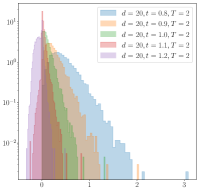
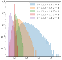
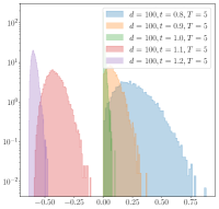
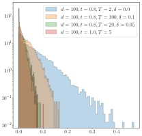
Figure 6: (a)-(c) Histograms of the normalized relative error across different temperatures $t$ and smoothing factors $T$ across different dimensions $d$. $\rho_{\text{\tiny$t$-dHG}}$ is an under (over) estimator of the true distance $\rho_{\text{\tiny$t$-HG}}$ for $t>1$ ($t<1$). Also, the relative approximation error is larger when $t$ deviates further from $1$. (d) The histograms of relative errors when using a mismatched temperature $1-\delta$ for the differentiable-max operator.

$T=1\,$

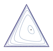
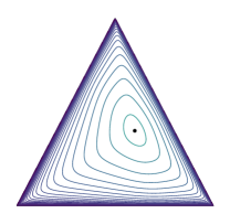
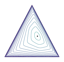
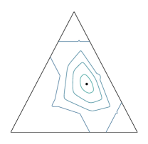
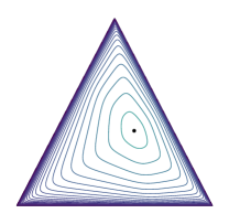
() $t=0.8$

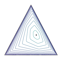
() $t=1.0$

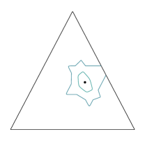
() $t=1.1$

Figure 7: Balls of different radii with respect to $\rho_{\text{\tiny$t$-dHG}}$ shown on the simplex for different temperature $t$ and smoothing factor $T$. The center is shown with a black dot. Darker colors indicate larger distances. Only when $t\leq 1$, we have $\rho_{\text{\tiny$t$-dHG}}\rightarrow\rho_{\text{\tiny$t$-HG}}$ as $T\rightarrow\infty$.

$T=10$

$T=20$

Appendix F Details of the Experiments on Comparing Different Geometries

We follow the procedure in Nielsen and Sun (2023) for comparing the quality of the embeddings. Let $\mathcal{M}^{d}$ denote the manifold that we use to embed a set of points from a dataset $\mathcal{D}$ and $\mathcal{Y}=\{\bm{y}_{i}\}_{i\in[n]}$ denote the embedding. Given the pairwise distances $D_{ij}$ between the points $i,j\in[n]$ in the original representation, we measure the embedding loss

$$\mathcal{L}(D,\mathcal{M}^{d})=\inf_{\mathcal{Y}\in(\mathcal{M}^{d})^{n}}\frac{1}{n^{2}}\sum_{i\in[n]}\sum_{j\in[n]}(D_{ij}-\rho_{\mathcal{M}}(\bm{y}_{i},\bm{y}_{j}))\,,$$ (56)

where $\rho_{\mathcal{M}}$ denotes the distance function of the geometry. We consider: i) Euclidean, ii) Minkowski hyperboloid model, iii) Hilbert simplex embedding, and iv) $t$-Hilbert co-simplex embedding. For Hilbert simplex embedding, we represent the points in log-coordinates. For $t$-Hilbert, we use the same $\log$-representation as Hilbert embedding but apply the function $x\mapsto\log_{t}\exp x$ on the Hilbert distance to convert the pairwise distances. We use PyTorch for the implementation and Adam as the optimizer. The details of the initialization and tuning follow Nielsen and Sun (2023) and are omitted.

Appendix G Tempered Klein and Poincaré Disk Models

The Klein model represents the hyperbolic plane as the interior of a unit ball. The distance between any two points $\bm{r}$ and $\bm{s}$ in the interior of the unit ball corresponds to Hilbert’s distance with $\chi=\frac{1}{2}$ and $\Omega=\{\bm{x}\in\mathbb{R}^{d}{\ :\ }\|\bm{x}\|_{2}<1\}$ as the convex domain (Richter-Gebert, 2011):

$$\rho_{\text{\tiny K}}(\bm{r},\bm{s})=\mathrm{arccosh}\left(\frac{1-\bm{r}\cdot\bm{s}}{\sqrt{(1-\bm{r}\cdot\bm{r})\,(1-\bm{s}\cdot\bm{s})}}\right)\,,$$

where $\bm{r}\cdot\bm{s}$ denotes the Euclidean inner-product and $\mathrm{arccosh}(x)=\log(x+\sqrt{x^{2}-1})$ for $x>1$. The geodesics in this model connecting any two points correspond to line segments, although the representation is non-conformal (i.e., it does not preserve the angles except at the disk origin).

Consider the map

$$\psi_{t,\chi}(u)=\chi\log_{t}\exp\frac{u}{\chi}\,,\,\,\chi>0\,.$$ (57)

Note that the map $\psi_{t,\chi}$ converts a given input $\log$-cross-ratio, scaled by $\chi$, into the $\log_{t}$ of the cross-ratio, scaled by the same factor $\chi$. Thus, to generalize the Klein model, we define the tempered Klein distance as

$$\rho_{t\text{\tiny-K}}(\bm{r},\bm{s})=\psi_{t,\nicefrac{{1}}{{2}}}(\rho_{\text{\tiny K}}(\bm{r},\bm{s}))\,.$$

Clearly, we have $\rho_{t\text{\tiny-K}}(\bm{r},\bm{s})\rightarrow\rho_{\text{\tiny K}}(\bm{r},\bm{s})$ as $t\rightarrow 1$.

The Poincaré disk model is a conformal representation also defined on the interior of a unit ball. In the Poincaré model, the distance between two points $\bm{r}$ and $\bm{s}$ in the domain is defined as

$$\rho_{\text{\tiny P}}(\bm{r},\bm{s})=\mathrm{arccosh}\left(1+2\,\frac{\|\bm{r}-\bm{s}\|^{2}_{2}}{\sqrt{(1-\|\bm{r}\|^{2}_{2})\,(1-\bm{s}\cdot\|\bm{s}\|^{2}_{2})}}\right)\,.$$

In this model, the straight lines in the hyperbolic geometry are represented by arcs of circles perpendicular to the unit ball (including straight line segments passing through the disk origin). We similarly define the tempered Poincaré distance as

$$\rho_{t\text{\tiny-P}}(\bm{r},\bm{s})=\psi_{t,\nicefrac{{1}}{{2}}}(\rho_{\text{\tiny P}}(\bm{r},\bm{s}))\,,$$

where similarly we have $\rho_{t\text{\tiny-P}}(\bm{r},\bm{s})\rightarrow\rho_{\text{\tiny P}}(\bm{r},\bm{s})$ as $t\rightarrow 1$. A point $\bm{k}$ in the Klein disk model is mapped to a point in the Poincaré disk via the radial rescaling map

$$\pi:\,\bm{k}\mapsto\frac{1-\sqrt{1-\|\bm{k}\|^{2}_{2}}}{\|\bm{k}\|^{2}_{2}}\,\bm{k}\,.$$ (58)

Since the tempered Klein distance $\rho_{t\text{\tiny-K}}$ is obtained from the Klein distance $\rho_{\text{\tiny K}}$ via the monotonic transformation $\psi_{t,\nicefrac{{1}}{{2}}}$, the same formula (58) maps the tempered Klein model to the tempered Poincaré model. We visualize several straight lines in the tempered Klein disk model that have identical distances between the start point $\bullet$ and the endpoint $\bm{\times}$ in Figure 8(a) for different $t$. Note that the value of the distance changes with $t$, but the distances are identical for the same value of $t$. We also show the point on the line that is $0.2\times$ away from the start point $\bullet$ relative to the total distance. The relative distance is dilated for $t<1$ and contracted $t>1$, compared to the Klein model. Similarly, we show these lines in the Poincaré model in Figure 8(b), where the same dilation and contraction of the distances are evident. We repeat the same procedure, but for a point $0.5\times$ away relative to the start point $\bullet$, located at the origin, for the Klein and Poincaré models in Figure 8(c) and (d), respectively.

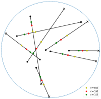
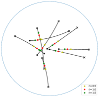
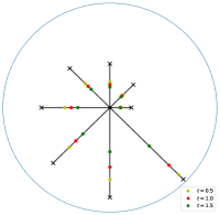
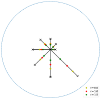
Figure 8: Visualization of straight lines in the Klein ((a) and (c)) and Poincaré ((b) and (d)) models. In (a) and (b), the lines have identical lengths, and the colored point indicates the point $0.2\times$ away from the start point $\bullet$ relative to the total length for different $t$. We similarly show the points $0.5\times$ away (midpoints) from the start point $\bullet$ relative to the total length in (c) and (d). The tempered distances represents a dilation for $t<1$ and a contraction for $t>1$.

References

• Amari and Ohara (2011) Shun-ichi Amari and Atsumi Ohara. Geometry of q-exponential family of probability distributions. Entropy, 13(6):1170–1185, 2011.
• Amari et al. (2012) Shun-ichi Amari, Atsumi Ohara, and Hiroshi Matsuzoe. Geometry of deformed exponential families: Invariant, dually-flat and conformal geometries. Physica A: Statistical Mechanics and its Applications, 391(18):4308–4319, 2012.
• Amid (2020) Ehsan Amid. Tempered Bregman Divergence for Continuous and Discrete Time Mirror Descent and Robust Classification. PhD thesis, University of California, Santa Cruz, 2020.
• Amid et al. (2023a) Ehsan Amid, Frank Nielsen, Richard Nock, and Manfred K Warmuth. Optimal transport with tempered exponential measures. arXiv preprint arXiv:2309.04015, 2023a.
• Amid et al. (2023b) Ehsan Amid, Richard Nock, and Manfred K Warmuth. Clustering above exponential families with tempered exponential measures. In International Conference on Artificial Intelligence and Statistics, pages 2994–3017. PMLR, 2023b.
• Arnaudon and Nielsen (2012) Marc Arnaudon and Frank Nielsen. Medians and means in Finsler geometry. LMS Journal of Computation and Mathematics, 15:23–37, 2012.
• Birkhoff (1957) Garrett Birkhoff. Extensions of Jentzsch’s theorem. Transactions of the American Mathematical Society, 85(1):219–227, 1957.
• Bregman (1967) Lev M Bregman. The relaxation method of finding the common point of convex sets and its application to the solution of problems in convex programming. USSR computational mathematics and mathematical physics, 7(3):200–217, 1967.
• Bushell (1973) P.-J. Bushell. Hilbert’s metric and positive contraction mappings in a Banach space. Arch. for Rational Mechanics and Analysis, 52:330–338, 1973.
• de la Harpe (2000) P. de la Harpe. Topics in Geometric Group Theory. Chicago Lectures in Mathematics. University of Chicago Press, 2000. ISBN 9780226317199.
• Doboš (1981) Ján Borsík—Jozef Doboš. Functions whose composition with every metric is a metric. Math. Slovaca, 31(1):3–12, 1981.
• Gezalyan and Mount (2023) Auguste H. Gezalyan and David M. Mount. Voronoi Diagrams in the Hilbert Metric. In Erin W. Chambers and Joachim Gudmundsson, editors, 39th International Symposium on Computational Geometry, SoCG 2023, June 12-15, 2023, Dallas, Texas, USA, volume 258 of LIPIcs, pages 35:1–35:16. Schloss Dagstuhl - Leibniz-Zentrum für Informatik, 2023. doi: 10.4230/LIPIcs.SoCG.2023.35. URL https://doi.org/10.4230/LIPIcs.SoCG.2023.35.
• Hilbert (1895) David Hilbert. Über die gerade Linie als kürzeste Verbindung zweier Punkte. Mathematische Annalen, 46(1):91–96, 1895.
• Hiriart-Urruty and Lemaréchal (2001) Jean-Baptiste Hiriart-Urruty and Claude Lemaréchal. Fundamentals of Convex Analysis. Springer-Verlag Berlin Heidelberg, first edition, 2001.
• Kohlberg and Pratt (1982) Elon Kohlberg and John W Pratt. The contraction mapping approach to the Perron-Frobenius theory: Why Hilbert’s metric? Mathematics of Operations Research, 7(2):198–210, 1982.
• Koolen et al. (2011) Wouter M Koolen, Wojciech Kotlowski, and Manfred K. K Warmuth. Learning eigenvectors for free. In Advances in Neural Information Processing Systems, volume 24. Curran Associates, Inc., 2011.
• Lemmens and Nussbaum (2014) Bas Lemmens and Roger D. Nussbaum. Birkhoff’s version of Hilbert’s metric and its applications in analysis. In Athanase Papadopoulos and Marc Troyanov, editors, Handbook of Hilbert geometry, pages 275–303. European Mathematical Society (EMS) press, 2014. ISBN 978-3-03719-147-7. doi: 10.4171/147-1/10. Chapter 10.
• Matveev (2012) Vladimir S Matveev. Can we make a Finsler metric complete by a trivial projective change? In Recent trends in Lorentzian geometry, pages 231–242. Springer, 2012.
• Naudts (2011) J. Naudts. Generalized thermostatistics. Springer, 2011.
• Naudts (2002) Jan Naudts. Deformed exponentials and logarithms in generalized thermostatistics. physica a, 316:323–334, 2002.
• Naudts (2004) Jan Naudts. generalized thermostatistics and mean-field theory. physica a, 332:279–300, 2004.
• Naudts (2009) Jan Naudts. The $q$-exponential family in statistical physics. Central European Journal of Physics, 7:405–413, 2009.
• Nielsen and Sun (2019) Frank Nielsen and Ke Sun. Clustering in Hilbert’s projective geometry: The case studies of the probability simplex and the elliptope of correlation matrices. Geometric structures of information, pages 297–331, 2019.
• Nielsen and Sun (2023) Frank Nielsen and Ke Sun. Non-linear Embeddings in Hilbert Simplex Geometry. In Timothy Doster, Tegan Emerson, Henry Kvinge, Nina Miolane, Mathilde Papillon, Bastian Rieck, and Sophia Sanborn, editors, Proceedings of 2nd Annual Workshop on Topology, Algebra, and Geometry in Machine Learning (TAG-ML), volume 221 of Proceedings of Machine Learning Research, pages 254–266. PMLR, 28 Jul 2023. URL https://proceedings.mlr.press/v221/nielsen23a.html. arXiv:2203.11434.
• Nivanen et al. (2003) L. Nivanen, A. Le Méhauté, and Q.-A. Wang. Generalized algebra within a nonextensive statistics. Reports on Mathematical Physics, 52:437–444, 2003.
• Nock et al. (2023) Richard Nock, Ehsan Amid, and Manfred K Warmuth. Boosting with Tempered Exponential Measures. In NeurIPS’23, 2023.
• Onishchik and Sulanke (2006) Arkadij L Onishchik and Rolf Sulanke. Projective and Cayley-Klein Geometries. Springer Science & Business Media, 2006.
• Papadopoulos (2014) Athanase Papadopoulos. Hilbert’s fourth problem. In Athanase Papadopoulos and Marc Troyanov, editors, Handbook of Hilbert geometry, pages 391–431. European Mathematical Society (EMS) press, 2014. ISBN 978-3-03719-147-7. doi: 10.4171/147-1/15. Chapter 15.
• Papadopoulos and Troyanov (2014) Athanase Papadopoulos and Marc Troyanov. Handbook of Hilbert geometry. European Mathematical Society (EMS) press, 2014. ISBN 978-3-03719-147-7. doi: 10.4171/147.
• Peyré and Cuturi (2019) Gabriel Peyré and Marco Cuturi. Computational optimal transport: With applications to data science. Foundations and Trends® in Machine Learning, 11(5-6):355–607, 2019.
• Richter-Gebert (2011) Jürgen Richter-Gebert. Perspectives on projective geometry: a guided tour through real and complex geometry. Springer, 2011.
• Shao and Nielsen (2017) Laëtitia Shao and Frank Nielsen. Machine Learning with Cayley-Klein metrics, 2017.
• Troyanov (2014a) Marc Troyanov. Funk and Hilbert geometries from the Finslerian viewpoint. In Athanase Papadopoulos and Marc Troyanov, editors, Handbook of Hilbert geometry, pages 69–110. European Mathematical Society (EMS) press, 2014a. ISBN 978-3-03719-147-7. doi: 10.4171/147-1/3. Chapter 3.
• Troyanov (2014b) Marc Troyanov. On the origin of Hilbert Geometry. In Athanase Papadopoulos and Marc Troyanov, editors, Handbook of Hilbert geometry, pages 383–389. European Mathematical Society (EMS) press, 2014b. ISBN 978-3-03719-147-7. doi: 10.4171/147-1/14. Chapter 14.
• Troyanov (2014c) Marc Troyanov. On the origin of hilbert geometry. arXiv preprint arXiv:1407.3777, 2014c.
• Tsallis (1988) Constantino Tsallis. Possible generalization of boltzmann-gibbs statistics. Journal of statistical physics, 52:479–487, 1988.