Abstract

Classifier-free guidance is a key component for enhancing the performance of conditional generative models across diverse tasks. While it has previously demonstrated remarkable improvements for the sample quality, it has only been exclusively employed for diffusion models. In this paper, we integrate classifier-free guidance into Flow Matching (FM) models, an alternative simulation-free approach that trains Continuous Normalizing Flows (CNFs) based on regressing vector fields. We explore the usage of Guided Flows for a variety of downstream applications. We show that Guided Flows significantly improves the sample quality in conditional image generation and zero-shot text-to-speech synthesis, boasting state-of-the-art performance. Notably, we are the first to apply flow models for plan generation in the offline reinforcement learning setting, showcasing a 10x speedup in computation compared to diffusion models while maintaining comparable performance.

1 Introduction

Conditional generative modeling paves the way to numerous machine learning applications such as conditional image generation (Dhariwal and Nichol, 2021; Rombach et al., 2022), text-to-speech synthesis (Wang et al., 2023; Le et al., 2023), and even solving decision making problems (Chen et al., 2021; Janner et al., 2021, 2022; Ajay et al., 2022). Models that appear ubiquitously across a variety of application domains are diffusion models (Sohl-Dickstein et al., 2015; Ho et al., 2020) and flow-based models (Song et al., 2020b; Lipman et al., 2023; Albergo and Vanden-Eijnden, 2022). Majority of this development has been focused around diffusion models, where multiple forms of conditional guidance Dhariwal and Nichol (2021); Ho and Salimans (2022) have been introduced to place larger emphasis on the conditional information. While flow models have been shown to be more efficient alternatives than diffusion models (Lipman et al., 2023; Pooladian et al., 2023) in unconditional generation, requiring less computation to sample, their behavior in conditional generation tasks has not been explored as much. It also remains unclear whether conditional guidance can be applied to and help the performance of flow-based models.

In this work, we study the behavior of Flow Matching models for conditional generation. We introduce Guided Flows, an adaptation of classifier-free guidance (Ho and Salimans, 2022) to Flow Matching models, showing that an analogous modification can be made to the velocity vector fields, including the optimal transport (Lipman et al., 2023) and cosine scheduling (Albergo and Vanden-Eijnden, 2022) flows used by prior works.

Application	data point $x_{1}$	conditioning variables $y$
Image Generation	image	class label
Text-to-Speech	spectrogram	text & utterance
Offline RL	state sequence	target return

Table 1.1: The data point $x_{1}$ and the conditioning variables $y$ on which the conditional guidance will be applied, for the three applications settings that we consider.

We experimentally validate Guided Flows on a variety of applications, ranging from generative modeling over multiple modalities to offline reinforcement learning (RL), see Table 1.1. As we show in Section 4, for standard generative tasks including image synthesis and zero-shot text-to-speech generation, Guided Flows significantly improves the sampling quality over unguided counterparts (i.e., sample from the conditional distribution directly), attaining state-of-the-art (SOTA) performance.

Particularly, the integration of guidance enables us to apply flow-based models for return-conditioned plan generating in offline RL for the first time. The evaluation of offline trained RL agents is via sequential online interactions. The usage of conditional generative models for plan generation (Janner et al., 2021, 2022; Ajay et al., 2022) often requires the model to accurately model not only relations within the training data set, but to also generalize to unseen conditional signals during online evaluation. There, we find that guided flows generate reliable execution plans, given the current state and a target return values. Guided Flows also obtain notably higher returns than unguided flows, achieving SOTA performance as well, see Section 5.3.

In addition to its efficacy, for all these aforementioned tasks, Guided Flows also demonstrate favorable compute efficiency and performance tradeoffs. Particularly, for offline RL, Guided Flows enjoys a remarkable 10x speed up compared with diffusion models.

2 Related Work

Diffusion and Flow Generative Models.

Recent major developments in generative models are on building simple models that are highly-efficient to train while providing the means of using conditional inference for solving downstream applications (Janner et al., 2022; Ajay et al., 2022; Kawar et al., 2022; Pokle et al., 2023; Le et al., 2023). The predominant progress in this domain has primarily centered on diffusion models (Sohl-Dickstein et al., 2015; Ho et al., 2020; Song et al., 2020b). Within these models, two types of conditional guidance (Dhariwal and Nichol, 2021; Ho and Salimans, 2022) can be employed to promote the conditional information. Whether these form of conditional guidance can be integrated into and help other types of generative models, remains an open question.

As two concurrent works, Dao et al. (2023) derive an approach similar to ours but is mainly motivated heuristically for the conditional optimal transport probability path; Hu et al. (2023) develop another different approach by adding an offset to the learned vector field, without theoretical guarantees on the sample distribution. It is noteworthy that we also show the efficacy of guidance in flows across a much wider variety of domain settings. In particular, our offline RL use case is quite different from the generative modeling tasks considered in those works.

Conditional Generative Modeling in Offline Reinforcement Learning.

Reinforcement learning (RL) is a powerful paradigm that has been widely applied to solve complex sequential decision making tasks, such as playing games Silver et al. (2016), controlling robotics Kober et al. (2013), dialogue systems Li et al. (2016); Singh et al. (1999). The premise of offline RL is to learn effective policies solely from static datasets that consist of previous collected experiences, generated by certain unknown policies Levine et al. (2020). There, the agent is not allowed to interact with the environment, thus subsides the potential risk and cost of online interactions for high-risk domains such as healthcare.

Conditional generative models are becoming handy tools to help decision making. A rich body of work Chen et al. (2021); Janner et al. (2021, 2022); Ajay et al. (2022); Zhao and Grover (2023); Zheng et al. (2023) focuses on modeling trajectories as sequences of state, action, and reward tokens. Instead of optimizing the expected return as the classic RL methods, the training objective of all these methods is to simply maximize the likelihood of sequences in the offline dataset. In essence, these methods cast RL as supervised sequence modeling problems, and generative models such as Transformer Vaswani et al. (2017); Radford et al. (2018), Diffusion Models Ho et al. (2020) thus come into play. Solving RL from this new perspective improves its training stability, and further opens the door of multimodal and multitask pretraining Zheng et al. (2022); Lee et al. (2022); Reed et al. (2022), similar to other domains like language and vision Radford et al. (2018); Chen et al. (2020a); Brown et al. (2020); Lu et al. (2022). There, a generative model can be used as a policy to autoregressively generate actions Chen et al. (2021); Zheng et al. (2022); alternatively, it can generate imagined trajectories which serves as execution plans given current state and a target output such as return or goal location Janner et al. (2021, 2022); Ajay et al. (2022); Zhao and Grover (2023). There are other works that replace the parameterized Gaussian policies in classic RL methods by generative models to facilitate the modeling of multimodal action distributions Wang et al. (2022); Chi et al. (2023); Ward et al. (2019). Akimov et al. (2022) apply flow-based models to offline RL as conservative action encoders (and decoders), which decode actions from latent variables output by the policy.

3 Guided Flow Matching

Setup.

Let $(x_{1},y)\sim q(x_{1},y)$ denote a true data point where $y\in\mathbb{R}^{k}$ is a conditioning variable; $x_{0}\sim p(x_{0})$ is a noise sample, where both data and noise reside in the same euclidean space, i.e., $x_{0},x_{1}\in\mathbb{R}^{d}$. Continuous Normalizing Flows (CNFs; Chen et al. 2018) define a map taking the noise sample $x_{0}$ to a data sample $x_{1}$ by first learning a vector field $u:[0,1]\times\mathbb{R}^{d}\times\mathbb{R}^{k}\rightarrow\mathbb{R}^{d}$ and second, integrating the vector field, i.e., solving the following Ordinary Differential Equation (ODE)

$$\dot{x}_{t}=u_{t}(x_{t}|y)$$ (1)

starting at $x_{0}$ for $t=0$ and solving until time $t=1$. For notation simplicity, we use subscript $t$ to denote the first input of function $u$.

Flow Matching (FM).

Lipman et al. (2023); Albergo and Vanden-Eijnden (2022) propose a method for efficient training of $u$ based on regressing a target velocity field. This target velocity field, denoted by $u:[0,1]\times\mathbb{R}^{d}\times\mathbb{R}^{k}\rightarrow\mathbb{R}^{d}$, takes noise samples $x_{0}$ and condition vectors $y$ to data samples $x_{1}$, i.e., it is constructed to generate the following marginal probability path

$$p_{t}(x|y)=\int p_{t}(x|x_{1})q(x_{1}|y)dx_{1},$$ (2)

where $p_{t}(\cdot|x_{1})$ is a probability path interpolating between noise and a single data point $x_{1}$. That is, $p_{t}(\cdot|x_{1})$ satisfies

$$p_{0}(\cdot|x_{1})\equiv p(\cdot),\qquad p_{1}(\cdot|x_{1})\approx\delta_{x_{1}}(\cdot),$$ (3)

where $\delta_{x_{1}}(\cdot)$ is the delta probability that concentrates all its mass at $x_{1}$. Note that $p_{0}\equiv p$ is the noise distribution. An immediate consequence of the boundary conditions in equation (3) is that $p_{t}(\cdot|y)$ indeed interpolates between noise and data, i.e., $p_{0}(\cdot|y)\equiv p(\cdot)$ and $p_{1}(\cdot|y)\approx q(\cdot|y)$ for all $y$.

Next, we assume $u_{t}(\cdot|x_{1})$ is a velocity field that generates $p_{t}(\cdot|x_{1})$ in the sense that solutions to equation (1), with $u_{t}(\cdot|x_{1})$ as the velocity field and $x_{0}\sim p(x_{0})$, satisfy $x_{t}\sim p_{t}(x_{t}|x_{1})$. The target velocity field for FM is then defined via

$$u_{t}(x|y)=\int u_{t}(x|x_{1})\frac{p_{t}(x|x_{1})q(x_{1}|y)}{p_{t}(x)}dx_{1},$$ (4)

and can be proved to generate, in the sense described above, the marginal probability path $p_{t}(\cdot|y)$ in equation (2). FM is trained by minimizing a tractable loss called the Conditional Flow Matching (CFM) loss (defined later), whose global minimizer is the target velocity field $u_{t}$.

Gaussian Paths.

A popular instantiation of paths $p_{t}(x|x_{1})$ are Gaussian paths defined by

$$p_{t}(x|x_{1})={\mathcal{N}}(x|\alpha_{t}x_{1},\sigma_{t}^{2}I),$$ (5)

where ${\mathcal{N}}$ is the Gaussian kernel, $\alpha,\sigma:[0,1]\rightarrow[0,1]$ are differentiable functions satisfying $\alpha_{0}=0=\sigma_{1}$, $\alpha_{1}=1=\sigma_{0}$. A pair $(\alpha_{t},\sigma_{t})$ is called a scheduler. Marginal paths $p_{t}(x|y)$ defined with $p_{t}(x|x_{1})$ as in equation (5) are called marginal Gaussian paths.

By convention we denote by $\varnothing$ the null conditioning and set $q(x):=q(x|\varnothing)$, $u^{\theta}_{t}(x):=u^{\theta}_{t}(x|\varnothing)$, and $u_{t}(x):=u_{t}(x|\varnothing)$.

Guided Flows.

Next, we adapt the notion of Classifier-Free Guidance (CFG; Ho and Salimans 2022) to conditional velocity fields $u_{t}(x|y)$. As in CFG, we set our goal to sample from the distribution $\tilde{q}(x|y)\propto q(x)^{1-\omega}q(x|y)^{\omega}$, $\omega\in\mathbb{R}$, where only explicit Flow Matching models for $q(x)$ and $q(x|y)$ are given. Motivated by CFG we define

$$\tilde{u}_{t}(x|y)=(1-\omega)u_{t}(x)+\omega u_{t}(x|y)$$ (6)

To justify this formula for velocity fields, we first relate $u_{t}(x|y)$ to the score function $\nabla\log p_{t}(x|y)$ using the following lemma proved in Appendix A.1:

Lemma 1

Let $p_{t}(x|y)$ be a Gaussian Path defined by a scheduler $(\alpha_{t},\sigma_{t})$, then its generating velocity field $u_{t}(x|y)$ is related to the score function $\nabla\log p_{t}(x|y)$ by

$$u_{t}(x|y)=a_{t}x+b_{t}\nabla\log p_{t}(x|y),$$ (7)

where

$$a_{t}=\frac{\dot{\alpha}_{t}}{\alpha_{t}},\qquad b_{t}=(\dot{\alpha}_{t}\sigma_{t}-\alpha_{t}\dot{\sigma}_{t})\frac{\sigma_{t}}{\alpha_{t}}.$$ (8)

Next, using this the lemma and plugging equation (7) for $u_{t}(x)=u_{t}(x|\varnothing)$ and $u_{t}(x|y)$ in the r.h.s. of equation (6), we get

$$\tilde{u}_{t}(x|y)=a_{t}x+b_{t}\nabla\log\tilde{p}_{t}(x|y),$$ (9)

where

$$\tilde{p}_{t}(x|y)\propto p_{t}(x)^{1-\omega}p_{t}(x|y)^{\omega}$$ (10)

is the geometric weighted average of $p_{t}(x)$ and $p_{t}(x|y)$.

As we prove in Appendix B, this velocity field $\tilde{u}_{t}$ coincides with the one in the Probability Flow ODE (Song et al., 2020b) used in Classifier Free Guidance for approximate sampling from distribution $\tilde{q}(\cdot|y)$. This provides a justification for equation (6). We note, however, that this analysis shows that both Guided Flows and CFG are guaranteed to sample from $\tilde{q}(\cdot|y)$ at time $t=1$ if the probability path $\tilde{p}_{t}(\cdot|y)$ defined in equation (10) is close to the marginal probability path $\int p_{t}(\cdot|x_{1})\tilde{q}(x_{1}|y)dx_{1}$, but it is not clear to what extent this assumption holds in practice.

Input: $p_{\text{uncond}}$ probability of unconditional training

Initialize $u_{t}^{\theta}$

while not converged do

       $(x_{1},y)\sim q(x_{1},y)$ $\triangleright$ sample data and condition

       $y\leftarrow\varnothing$ with probability $p_{\text{uncond}}$ $\triangleright$ null condition

       $x_{0}\sim p(x_{0})$ $\triangleright$ sample noise

       $x_{t}\leftarrow\alpha_{t}x_{1}+\sigma_{t}x_{0}$ $\triangleright$ noisy data point

       $\dot{x}_{t}\leftarrow\dot{\alpha}_{t}x_{1}+\dot{\sigma}_{t}x_{0}$ $\triangleright$ derivative of noisy data point

       Take gradient step on $\nabla_{\theta}\left\|u^{\theta}_{t}(x_{t},y)-\dot{x}_{t}\right\|^{2}$

Output: $u_{t}^{\theta}$

Algorithm 1 Training Guided Flows

Training Guided Flows.

Training guided flow follows the practice in CFG but replaces the Diffusion training loss with the Conditional Flow Matching (CFM) loss (Lipman et al., 2023). This leads to the following loss function:

where $t$ is sampled uniformly in $[0,1]$, $b\sim\text{Bernoulli}(p_{\text{uncond}})$ is used to indicate whether we will use null condition, $x_{1}$ and $y$ are sampled from the true data distribution, $x_{t}=\alpha_{t}x_{1}+\sigma_{t}x_{0}$, $\dot{x}_{t}=u_{t}(x_{t}|x_{1})=\dot{\alpha}_{t}x_{1}+\dot{\sigma}_{t}x_{0}$ and $u^{\theta}:[0,1]\times\mathbb{R}^{d}\times\mathbb{R}^{k}\rightarrow\mathbb{R}^{d}$ is a neural network with learnable parameters $\theta\in\mathbb{R}^{p}$. The training process is summarized in Algorithm 1.

Sampling Guided Flows.

Sampling from Guided Flows required approximating the solution to the sampling ODE (equation (1)) with the guided velocty field $\tilde{u}_{t}$ defined in equation (6), see Algorithm 2.

Illustrative Example.

Figure 3.1 shows a visualization of the effect of Guided Flows in a toy 2D example of a mixture of Gaussian distributions, where $y$ is the latent variable specifying the identity of the mixture component, and $q(x_{1}|y)$ is one single Gaussian component. When the guidance weight is $1.0$, there is no guidance performed, and we are sampling from the unconditional marginal $q(x_{1})$. We see that as guidance weight increases, the samples move away from the unconditional distribution $q(x_{1})$.

Input: trained velocity field $u^{\theta}_{t}$, condition $y$, guidance parameter $\omega$, number of ODE steps $n_{\text{ode}}$

$x_{0}\sim p(x_{0})$ $\triangleright$ sample noise

$h\leftarrow\frac{1}{n_{\text{ode}}}$ $\triangleright$ step size

$\tilde{u}_{t}(\cdot)\leftarrow(1-\omega)u^{\theta}_{t}(\cdot)+\omega u^{\theta}_{t}(\cdot|y)$ $\triangleright$ guided velocity

for $t=0,h,\ldots,1-h$ do

       $x_{t+h}\leftarrow$ ODEStep($\tilde{u}_{t}$, $x_{t}$) $\triangleright$ ODE solver step

      

Output: $x_{1}$

Algorithm 2 Sampling from Guided Flows

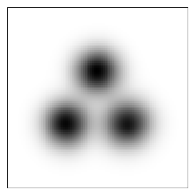
$w=1.0$

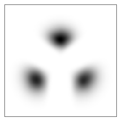
$w=2.0$

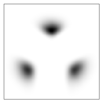
$w=3.0$

$w=4.0$

Figure 3.1: The effect of increasing guidance weight, conditioned on cluster index. Conditional guidance for all three clusters are shown simultaneously on the same plots.

4 Conditional Generative Modeling

In this section, we perform experiments to test whether Guided Flows can help achieve better sample quality than unguided models. In particular, we consider two application settings: conditional image generation and zero-shot text-to-speech synthesis. The goal of these experiments to test Guided Flows on standard generative modeling settings, where the evaluation is purely based on sample quality, while exploring different data modalities, before we move on validating Guided Flows for more complex planning tasks in Section 5.

4.1 Conditional Image Generation

1.0

Brambling

Husky

2.0

3.0

1.0

Meerkat

Otter

2.0

3.0

Figure 4.1: Generated samples from face-blurred ImageNet using four different class labels, showing the effect of different guidance weights with Guided Flows. Higher guidance weights result in more class-specific features to appear.

We downsample the official face-blurred ImageNet dataset to images of 64×64 pixels, using the open source preprocessing scripts from Chrabaszcz et al. (2017). We train Guided Flow Matching models $p_{t}(x|y)$ where $x$ denotes an image and $y$ is the class label of that image. In particular, we consider two affine Gaussian probability paths, the optimal transport (FM-OT) path considered by Lipman et al. (2023) and the cosine scheduling (FM-CS) path considered by Albergo and Vanden-Eijnden (2022). As a baseline, we train diffusion models (DDPM; Ho et al. 2020; Song et al. 2020b) with classifier-free guidance (Ho and Salimans, 2022). We report the results of both standard sampling of DDPM and also the deterministic DDIM sampling algorithm (Song et al., 2020a). All the models have the same U-Net architecture adopted from Dhariwal and Nichol (2021), and trained with the same hyperparameters and number of iterations, as listed in Table D.1.

Results are displayed in Figure 4.2. We see that guidance for Flow Matching models can drastically help increase sample quality (reducing FID from $2.54$ to $1.68$) using a midpoint solver with 200 number of function evaluations (NFE), i.e. 200 ODE steps. We do see that the optimal guidance weight can change depending on the compute cost (NFE), with NFE=10 having a higher optimal guidance weight. Additionally, in Figure 2(b) we show the Pareto front of the sample quality and efficiency tradeoff, plotted for each model. We note that the optimal guidance weight can be very different between each model, with DDPM noticeably requiring a larger guidance weight. Here we find that FM-OT models are slightly more efficient than the other models that we consider.

(a) Guidance

(b) Efficiency

Figure 4.2: (a) The performance of Guided Flows (FM-OT) as the guidance weight $\omega$ changes. When $\omega=0$, there is no guidance performed; with $\omega>1.0$, Guided Flows (FM-OT) achieve a lower FID. This trend is consistent when we use different NFEs (ODE steps). With NFE=200, the guided flow achieves FID $1.68$ on ImageNet-64.(b) Guided Flows with conditional optimal transport paths have the best tradeoff for efficiency, compared with other baselines.

4.2 Zero-shot Text-to-Speech Synthesis

Guidance Weight	Continuation	Text-only
Le et al. (2023)	2.00	3.10
1.0	2.06	3.09
1.2	1.95	2.98
1.4	1.96	2.89
1.6	1.95	2.83
1.8	1.94	2.87
2.0	1.98	2.82
2.2	1.96	2.80
2.4	2.10	2.83
2.6	2.40	2.76
2.8	3.40	2.79
3.0	5.10	2.75

Table 4.1: Word error rates (WER) for zero-shot text-to-speech. When the weight is $1.0$, there is no guidance performed and we sample directly from the trained conditional distribution. We see that performance improves when using Guided Flows with weights greater than 1.0.

Given a target text and a transcribed reference audio as conditioning information $y$, zero-shot text-to-speech (TTS) aims to synthesize speech resembling the audio style of the reference, which was never seen during training. As our Guided Flow model, we train a model on 60K hours ASR-transcribed English audiobooks, following the experiment setup in Le et al. (2023).

Specifically, we consider two main tasks. The first one is zero-shot TTS where the first 3 seconds of each utterance is provided and the model is requested to continue the speech. The second one is diverse speech generation, where only the text is provided to the model. In order to assess the accuracy of the generated results, we report the word error rate (WER) using automatic speech recognition (ASR) models following prior works (Wang et al., 2018).

Results of Guided Flows is provided in Table 4.1, where we also provide the results of Le et al. (2023) as reference. We also report our results when no guidance is used (weight equal to 1.0). With guidance, we see a marginal improvement for the continuation TTS task, and a much more sizable gain in the text-only TTS task. This likely due to the text-only TTS task being a much more diverse distribution.

5 Planning for Offline RL

5.1 Preliminaries

We model our environment as a Markov decision process (MDP) (Bellman, 1957) denoted by $\langle\mathcal{S},\mathcal{A},p,P,R,\gamma\rangle$, where $\mathcal{S}$ is the state space, $\mathcal{A}$ is the action space, $p(s_{0})$ is the distribution of the initial state, $P(s_{t+1}|s_{t},a_{t})$ is the transition probability distribution, $R(s_{t},a_{t})$ is the deterministic reward function, and $\gamma$ is the discount factor. At timestep $t$, the agent observes a state $s_{t}\in\mathcal{S}$ and executes an action $a_{t}\in\mathcal{A}$. The environment will provide the agent with a reward $r_{t}=R(s_{t},a_{t})$, and also moves it to the next state $s_{t+1}\sim P(\cdot|s_{t},a_{t})$. Let $\tau$ be a trajectory. For any length-$H$ subsequence $\tau_{\text{sub}}$ of $\tau$, e.g., from timestep $t$ to $t+H-1$, we define the return-to-go (RTG) of $\tau_{\text{sub}}$ to be the sum of its discounted return $g(\tau_{\text{sub}})=\sum_{t^{\prime}=t}^{t+H-1}\gamma^{t^{\prime}-t}r_{t^{\prime}}$. We also use $\bm{s}(\tau_{\text{sub}})$ to denote the state sequence extracted from the subsequence $\tau_{\text{sub}}$. A deterministic inverse dynamics model (IDM) is a function $f:\mathcal{S}\times\mathcal{S}\mapsto\mathcal{A}$ which predicts action using states: $\widehat{a}_{t}=f(s_{t},s_{t+1})$.

5.2 Our Setup

Input: trained conditional sequence model $p_{\theta}(s_{t+1},\ldots,s_{t+H-1}|s_{t},g_{t})$, IDM $f_{\rho}(s,s^{\prime})$, initial state $s_{0}$, initial conditioning parameter $g_{0}$, conditioning parameter updating rule $G$

$t\leftarrow 0$

while episode not done do

       Sample $(\widehat{s}_{t+1},\ldots,\widehat{s}_{t+H-1})\sim p_{\theta}(\cdot|s_{t},g_{t})$

       Predict action $\widehat{a}_{t}=f_{\rho}(s_{t},\widehat{s}_{t+1})$

       Execute $\widehat{a}_{t}$ and observe $s_{t+1}$ and $r_{t}$

       $g_{t+1}\leftarrow$ compute the next conditioning parameter according to $G$

       $t\leftarrow t+1$

      

Algorithm 3 A General Framework of Conditioned Generative Planning

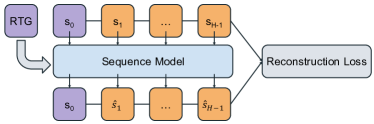
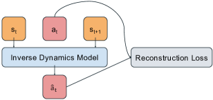
Figure 5.1: The training phase of return-conditioned generative planning. The state sequence model is trained in a classifer-free manner—with certain probability, it is conditioned on the RTG.

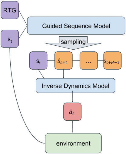
Figure 5.2: The evaluation phase using return-conditioned generative planning.

We consider the paradigm proposed by Ajay et al. (2022), where a generative model learns to predict a sequence of future states, conditioning on the current state and target output such as expected return. Intuitively, the predicted future states form a plan to reach the target output, and the predicted next state can be interpreted as the next intermediate goal on the roadmap. Based on the current state and the predicted next state, we use an inverse dynamics model to predict the action to execute. Algorithm 3 summarizes this framework. We emphasize that the target output $g_{t}$ is the conditioning variable where guidance will perform, and the current state $s_{t}$ is a general conditioning variable. In this work, we consider the target return as our conditioning variable. Return-conditioned RL methods are widly used to solve standard RL problems where the environment produces dense rewards Srivastava et al. (2019); Kumar et al. (2019); Schmidhuber (2019); Emmons et al. (2021); Chen et al. (2021); Nguyen et al. (2022). Figure 5.1 and 5.2 plot the training and evaluation phases of our paradigm. Careful readers might notice that we resample the whole sequence $\widehat{s}_{t+1},\ldots,\widehat{s}_{t+H-1}$ at every timestep $t$, but only use $\widehat{s}_{t+1}$ to predict $\widehat{a}_{t}$. In fact, it is completely feasible to predict the actions for the next multiple steps using a single plan, which also saves computation. We note that replanning at every timestep is for the sake of planning accuracy, as the error will accumulate as the horizon expands, and there is a tradeoff between computational efficiency and agent performance. For diffusion models, previous works have used heuristics to improve the execution speed, e.g., reusing previously generated plans to warm-start the sampling of subsequence plans Janner et al. (2022); Ajay et al. (2022). This is beyond the scope of our paper, and we only consider replanning at every timestep for simplicity.

5.3 Experiments

Our experiments aim at answering the following questions:

1. Can conditional flows generate meaningful plans for RL problems given a target return?

2. How do flows compare to diffusion models, in terms of both downstream RL task performance and compute efficiency?

3. Compared with unguided flows, can guidance help planning?

Tasks and Datasets

We consider three Gym locomotions tasks, hopper, walker and halfcheetah, using offline datasets from the D4RL benchmark Fu et al. (2020). For all the experiments, we train 5 instances of each method with different seeds. For each instance, we run 20 evaluation episodes. We shall discuss the model architectures and important hyperparameters below, and we refer the readers to Appendix E for more details.

Baseline

We compare our method to Decision Diffuser Ajay et al. (2022), which uses the same paradigm with diffusion models to model the state sequences.

Sequence Model Architectures

For the locomotion tasks, we train flows for state sequences of length $H=64$, parameterized through the velocity field $u^{\theta}$. Similar to the previous work Janner et al. (2022); Ajay et al. (2022), the velocity field $u^{\theta}$ is modeled as a temporal U-Net consisting of repeated convolutional residual blocks. Both the time $t$ and the RTG $g(\bm{s})$ are projected to latent spaces via multilayer perceptrons, where $t$ is first transformed to its sinusoidal position encoding. For the baseline method, the diffusion model is training similarly with $200$ diffusion steps, where we use a temporal U-Net to predict the noise at each diffusion steps throughout the diffusion process.

Inverse Dynamic Model

For all the environments and datasets, we model the IDM by an MLP with 2 hidden layers and 1024 hidden units per layer. Among all the offline trajectories, we randomly sample 10% of them as the validation set. We train the IDM for 100k iterations, and use the one that yields the best validation performance.

Low Temperature Sampling

To sample from the diffusion model, we use $200$ diffusion steps. For the sake of fair comparison, we also use $200$ ODE steps when sampling from the flow matching model. Following Ajay et al. (2022), we use the low temperature sampling technique for diffusion model, where at each diffusion step $k$ we sample the state sequence from $\mathcal{N}(\widehat{\mu}_{k},\alpha^{2}\widehat{\Sigma}_{k})$ with a hand-selected temperature parameter $\alpha\in(0,1)$. We sweep over 3 values of $\alpha$ for all our experiments: $0.1,0.25$, and $0.5$. For flow matching, we analogously set the initial distribution $p_{0}(x_{0})=\mathcal{N}(0,\nu^{2}I)$ and we sweep over two values of $\nu$: $0.1$ and $1$.

	hopper			walker			halfcheetah			Average
	medium-replay	medium	medium-expert	medium-replay	medium	medium-expert	medium-replay	medium	medium-expert
Flow	0.89	0.84	1.05	0.78	0.77	0.94	0.42	0.49	0.97	0.79
Diffusion	0.87	0.72	1.09	0.64	0.8	1.07	0.48	0.41	0.95	0.78

Table 5.1: The normalized return obtained when the state sequence models are trained by flows and diffusion models. We use the same IDM for both methods. Results aggregated over 5 training instances with different seeds.

5.3.1 Plan Generation (Q1)

To verify the capability of flows to generate meaningful plans that can guide the agent, we sample from a flow on the hopper-medium dataset. We randomly select a subtrajectory $\tau_{\text{sub}}$ from the dataset, and let flow condition on its first state and RTG $0.8$. Figure 5.3 plots both state sequences. We can see that the generated state sequence is almost identical to the ground truth, demonstrating that guided flow is capable to generate meaningful plans to navigate the agent. We note that this RTG value $0.8$ is out-of-distribution (OOD), as the maximum RTG value of the training dataset is $0.61$. This suggests that guided flows might be even robust to OOD RTG values, which we believe is an interesting property to understand and a potential direction to explore for future work, see related discussions in Chen et al. (2021); Emmons et al. (2021); Zheng et al. (2022); Nguyen et al. (2022). We refer the readers to Figure F.1 for more examples of generated plans.

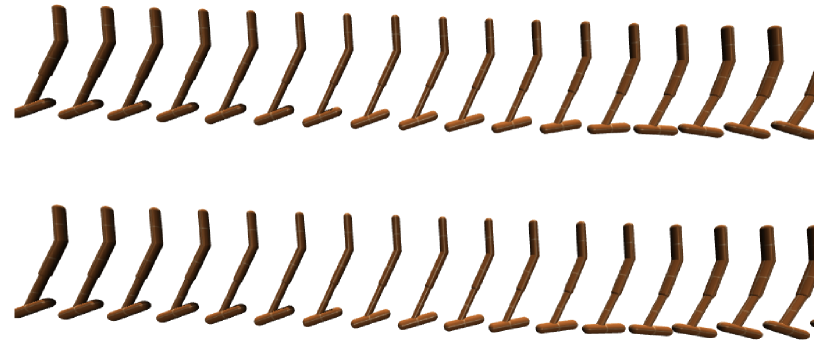
Figure 5.3: The top panel plots a truth state sequence $s_{0},s_{,}1\ldots$ randomly sampled from the hopper-medium dataset. The bottom panel plots the flow generated state sequence, conditioning on the first state $s_{0}$ with guidance weight $3.0$. These two sequences are very similar, demonstrating that guided flow is capable to generate meaningful plans to navigate the agent.

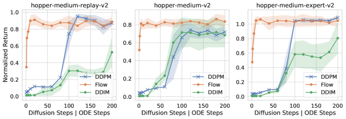
Figure 5.4: The obtained normalized return when the internal samplling steps used to generate the state sequence varies.

5.3.2 Benchmark (Q2)

In this section, we conduct experiments to investigate the efficacy and efficiency of guided flows. We highlight the predominant trends from our findings:

     Guided flows are on par with diffusion models with respect to the absolute performance, with a significant 10x speed up in sampling.

Performance Efficacy

Throughout all our experiments, in addition to the temperature parameter for sampling, for both methods, we sweep over 3 values of RTG: 0.4, 0.5, and 0.6 for the medium-replay and medium datasets of halfcheetah, and 0.7, 0.8 and 0.9 for all the other datasets. We also sweep over 4 values of guidance parameters: $1.8,2.0,2.2,2.4$ for diffusion models, and $1.0,1.5,2.0,2.5$ for flows. We train both guided flows and guided diffusion models for 2 million iterations, and save checkpoints every $200k$ iteration. We evaluate the performance on all the saved checkpoints and report the best result in Table 5.1. The performances of flow matching and diffusion model are comparable, where flow matching performs marginally better.

Computational Efficiency

A well-known pain-point of diffusion model is its computational inefficiency, since sampling from a diffusion model consists of iterative denoising steps. In our case, the diffusion model is trained with $200$ diffusion steps, thus it takes $200$ internal sampling steps to generate a sample with full quality. To accelerate sampling, many algorithms have been proposed to reduce the number of internal steps, including implicit models with deterministic sampling (DDIM,  Song et al. 2020a), distillation Salimans and Ho (2022), noise schedule Chen et al. (2020b); Nichol and Dhariwal (2021); Lin et al. (2023). As a tradeoff, these methods all lead to loss in sample quality. Similarly, sampling from a flow model requires a number of internal steps to solve the ODE equation (1), and more internal steps leads to sample with better quality.

To understand the computation-vs-quality tradeoff for both flows and diffusion models, we run an ablation experiment for the hopper task, where we only sample with $K$ internal steps $(K\leq 200)$ for both methods. In addition to the standard diffusion model (DDPM, Ho et al. (2020)), we also compare with DDIM Song et al. (2020a), a deterministic sampling algorithm widely used in diverse domains. Figure 5.4 plots the normalized return we obtain versus the number of internal steps. For all 3 datasets, phase transitions occur for all three methods. Surprisingly, $10$ ODE steps are sufficient for flows to generate samples leading to the same return as $200$ ODE steps; whereas DDPM and DDIM both need $100$ diffusion steps. Again, the performance of flows is comparable to DDPM and is better than DDIM. Next, we compare the CPU time consumed by these methods. Figure 5.5 shows that the CPU time consumed by the diffusion model and the flow are roughly the same when the number of internal steps match, and it scales linearly as the number of internal steps increase. This means, compared with diffusion model, flows only need $10\%$ computing time to generate samples leading to the same downstream performance. The trend remains the same when the batch size increase, see Figure F.2.

Figure 5.5: The CPU time of generating a batch of $704$-dimensional vectors (the subsequence length is 64, and each state is of dimension 11), where the batch size is $20$. Results averaged over $100$ replications.

5.3.3 Influence of Guidance (Q3)

Table 5.2 reports the normalized return obtained by our agents for the hopper and halfcheetah tasks, where the guidance weight varies from 1.0 to 3.0. The flows are trained on both medium and medium-replay datasets for hopper, and the medium dataset for halfcheetah. The guidance weight $1.0$ yields unguided flows. The results show that the guided flows outperform the unguided ones on all three datasets.

Guidance Weight	hopper		halfcheetah
	medium	medium-replay	medium
1.0	0.64	0.83	0.48
1.5	0.73	0.87	0.48
2.0	0.81	0.89	0.49
2.5	0.81	0.86	0.46
3.0	0.84	0.84	0.45

Table 5.2: The normalized return obtained when using different guidance weights. For both tasks, guided flows outperform unguided flows (guidance weight is $1$).

6 Conclusion

We thoroughly explore the theory and effect of guidance for flow matching. We empirically validate the conditional generative capabilities of flow-based models trained through recently-proposed simulation-free algorithms (Lipman et al., 2023; Albergo and Vanden-Eijnden, 2022) for a variety of applications, confirming its success across diverse domains. Our experiments show that conditional guidance can lead to better results for flow-based models. Moreover, guided flows excel in standard generative tasks like image synthesis and speech generation, achieving SOTA performance. Additionally, our experiments highlight both the efficacy and efficiency of guided flows in model-based planning: a significant 10x speedup in offline RL with performance on par with diffusion models. This underscores the great potential of flow matching in extending the application of generative models to planning problems, especially those demanding enhanced computational efficiency, such as online planning.

Acknowledgments

The authors thank Zihan Ding, Maryam Fazel-Zarandi, Brian Karrer, Maximilian Nickel, Mike Rabbat, Yuandong Tian, Amy Zhang, and Siyan Zhao for insightful discussions.

Appendix A Proofs

A.1 Proof of Lemma 1

See 1

Proof (Lemma 1). The Gaussian probability path $p_{t}(x|y)$ as in equation (2) is

$$p_{t}(x|y)=\int p_{t}(x|x_{1})q(x_{1}|y)dx_{1},$$ (12)

where $p_{t}(x|x_{1})={\mathcal{N}}(x|\alpha_{t}x_{1},\sigma_{t}^{2}I)$. We express the score function as

$$\nabla\log p_{t}(x|y) =\frac{\nabla p_{t}(x|y)}{p_{t}(x|y)}$$ (13)

$$=\int\frac{\nabla p_{t}(x|x_{1})q(x_{1}|y)}{p_{t}(x|y)}dx_{1}$$ (14)

$$=\int\nabla\log p_{t}(x|x_{1})\frac{p_{t}(x|x_{1})q(x_{1}|y)}{p_{t}(x|y)}dx_{1}.$$ (15)

The generating velocity field $u_{t}$ as in equation (4) is

$$u_{t}(x|y)=\int u_{t}(x|x_{1})\frac{p_{t}(x|x_{1})q(x_{1}|y)}{p_{t}(x|y)}dx_{1},$$ (16)

where $u_{t}(x|x_{1})=\frac{\dot{\sigma}_{t}}{\sigma_{t}}(x-\alpha_{t}x_{1})+\dot{\alpha}_{t}x_{1}$. Hence, by linearity of integrals it is enough to show that

$$u_{t}(x|x_{1})=\frac{\dot{\alpha}_{t}}{\alpha_{t}}x+(\dot{\alpha}_{t}\sigma_{t}-\alpha_{t}\dot{\sigma}_{t})\frac{\sigma_{t}}{\alpha_{t}}\nabla\log p_{t}(x|x_{1}).$$ (17)

And indeed,

$$u_{t}(x|x_{1}) =\frac{\dot{\sigma}_{t}}{\sigma_{t}}(x-\alpha_{t}x_{1})+\dot{\alpha}_{t}x_{1}$$ (18)

$$=\frac{\dot{\alpha}_{t}}{\alpha_{t}}x-\frac{\dot{\alpha}_{t}}{\alpha_{t}}x+\frac{\dot{\sigma}_{t}}{\sigma_{t}}(x-\alpha_{t}x_{1})+\dot{\alpha}_{t}x_{1}$$ (19)

$$=\frac{\dot{\alpha}_{t}}{\alpha_{t}}x-(\dot{\alpha}_{t}\sigma_{t}-\alpha_{t}\dot{\sigma}_{t})\frac{1}{\alpha_{t}\sigma_{t}}\left(x-\alpha_{t}x_{1}\right)$$ (20)

$$=\frac{\dot{\alpha}_{t}}{\alpha_{t}}x+(\dot{\alpha}_{t}\sigma_{t}-\alpha_{t}\dot{\sigma}_{t})\frac{\sigma_{t}}{\alpha_{t}}\nabla\log p_{t}(x|x_{1}),$$ (21)

where in the last equality we used our assumption of Gaussian probability path that gives $\nabla\log p_{t}(x|x_{1})=-\frac{1}{\sigma_{t}^{2}}(x-\alpha_{t}x_{1})$. $\square$

Appendix B Probability Flow ODE for Scheduler $(\alpha_{t},\sigma_{t})$

In this section we provide the velocity field used in CFG (Ho and Salimans, 2022) for approximate sampling from the conditional distribution $\tilde{q}(x|y)\propto q(x)^{1-\omega}q(x|y)^{\omega}$, $\omega\in\mathbb{R}$, and show that it coincides with our velocity field in equation (9).

We assume the marginal probability paths (see equation (2)) $p_{t}(x)$ and $p_{t}(x|y)$ are defined with a scheduler $(\alpha_{t},\sigma_{t})$ and data distribution $q(x)$ and $q(x|y)$, respectively. CFG consider the probability path

$$\tilde{p}_{t}(x|y)=p_{t}(x)^{1-\omega}p_{t}(x|y)^{\omega}$$ (22)

with the corresponding score function

$$\nabla\log\tilde{p}_{t}(x|y)=(1-\omega)\nabla p_{t}(x)+\omega\nabla p_{t}(x|y).$$ (23)

Then the sampling is done with the Probability Flow ODE of diffusion models (Song et al., 2020b),

$$\dot{x}_{t}=f_{t}x_{t}-\frac{1}{2}g_{t}^{2}\nabla\log\tilde{p}_{t}(x_{t}|y),$$ (24)

where $f_{t}=\frac{d\log\alpha_{t}}{dt}$, $g_{t}^{2}=\frac{d\sigma_{t}^{2}}{dt}-2\frac{d\log\alpha_{t}}{dt}\sigma_{t}$ (Kingma et al., 2023; Salimans and Ho, 2022). Lastly,

$$\frac{d\log\alpha_{t}}{dt}=\frac{\dot{\alpha}_{t}}{\alpha_{t}}=a_{t},\quad-\frac{1}{2}\frac{d\sigma_{t}^{2}}{dt}+\frac{d\log\alpha_{t}}{dt}\sigma_{t}=(\dot{\alpha}_{t}\sigma_{t}-\alpha_{t}\dot{\sigma}_{t})\frac{\sigma_{t}}{\alpha_{t}}=b_{t},$$ (25)

plugging this in equation (24) is an ODE with a velocity field that coincides with the velocity field in equation (9).

Appendix C Flow Matching Sampling with Guidance for Offline RL

Comparing with standard generative modeling, the sequence model trained for RL needs to condition on the current state $s_{t}$, see Section 5. Therefore, the sampling process is slightly different from Algorithm 2, as we need to zero out the vector fields corresponding to $s_{t}$, as shown in Algorithm 4. Sampling for the goal-conditioned model can be done similarly.

Input: initial state $s_{0}$, target return $R$, guidance parameter $\omega$, standard deviation of the starting distribution $\sigma$, number of ODE steps $n_{\text{ode}}$

Sample $x_{0}\sim\mathcal{N}(0,\sigma^{2}I)$

$h\leftarrow 1/n_{\text{ode}}$ $\triangleright$ step size

for $t=0,h,\ldots,1-h$ do

       $x_{t}[0]\leftarrow s_{0}$ $\triangleright$ fix the known token

       $\tilde{u}_{t}(\cdot)\leftarrow(1-\omega)u^{\theta}_{t}(\cdot)+\omega u^{\theta}_{t}(\cdot|R)$ $\triangleright$ compute the velocity field under guidance

       Define $\bar{u}_{t}(\cdot):\mathbb{R}^{p}\mapsto\mathbb{R}^{p}$ such that for any $x\in\mathbb{R}^{p}$, the first dimension of $\bar{u}_{t}(x)$ is equal to $0$, and the other dimensions are the same as $\tilde{u}_{t}(x)$ $\triangleright$ zero out the VF for the known token

       $x_{t+h}\leftarrow$ ODEStep$(\bar{u}_{t},x_{t})$

      

Output: $x_{1}$

Algorithm 4 Flow Matching Sampling with Guidance for Offline RL

Appendix D Image Generation Experiment Details

We train three models on ImageNet-64: DDPM (using noise prediction), FM-CS, and FM-OT.

FM-CS and FM-OT models are trained with the loss function in equation (11):

$$\mathbb{E}_{t,b,q(x_{1},y),p(x_{0})}\left\|u^{\theta}_{t}(x_{t}|(1-b)\cdot y+b\cdot\varnothing)-\dot{x}_{t}\right\|^{2},$$ (26)

where $t$ is sampled uniformly in $[0,1]$, $b\sim\text{Bernoulli}(p_{\text{uncond}})$ is used to indicate whether we will use null condition, $x_{0}$ is the noise, $x_{1}$ and $y$ are sampled from the true data distribution, and $x_{t}=\alpha_{t}x_{1}+\sigma_{t}x_{0}$, $\dot{x}_{t}=u_{t}(x_{t}|x_{1})=\dot{\alpha}_{t}x_{1}+\dot{\sigma}_{t}x_{0}$. The noise scheduler of FM-CS is the cosine scheduler Albergo and Vanden-Eijnden (2022):

$$\alpha_{t}=\sin\frac{\pi}{2}t,\qquad\sigma_{t}=\cos\frac{\pi}{2}t,$$ (27)

and the noise scheduler of FM-OT Lipman et al. (2023) is

$$\alpha_{t}=t,\qquad\sigma_{t}=1-t.$$ (28)

DDPM models are trained with noise prediction loss as derived in Ho et al. (2020) and Song et al. (2020b):

$$\mathbb{E}_{t,b,q(x_{1},y),p(x_{0})}\left\|{\epsilon}^{\theta}_{t}(x_{t}|(1-b)\cdot y+b\cdot\varnothing)-x_{0}\right\|^{2}.$$ (29)

We note that in our implementation, $t$ is sampled uniformly in $[0,1]$. We use the VP scheduler

$$\alpha_{t}=1-\zeta_{1-t},\qquad\sigma_{t}=\sqrt{1-\zeta^{2}_{1-t}},\qquad\zeta_{s}=\exp{-\frac{1}{4}s^{2}(c_{1}-c_{2})-\frac{1}{2}sc_{2}},$$ (30)

with $c_{1}=20$ and $c_{2}=0.1$.

All three models have the same U-Net architecture adopted from Dhariwal and Nichol (2021), with hyperparameters listed below. For all the methods, we sweep the guidance weight across the range of 1.0 to 2.0 with a grid size of 0.05, and report the best results in Figure 2(b). In particular, we have reported DDPM, DDIM and FM-CS using guidance weight 0.2, and FM-OT using guidance weight 0.15.

hyperparameter	value
channels	196
depth	3
channels multiple	1, 2, 3, 4
heads	-
heads channels	64
attention resolution	32, 16, 8
dropout rate	0.1
batch size	2048
learning rate	1e-4
learning rate scheduler	constant
iterations	$10^{6}$
$p_{\text{uncond}}$	0.2

Table D.1: Hyperparameters used to train diffusion models and flow models on the ImageNet-64 dataset.

Appendix E Offline RL Experiment Details

We summarize the architecture and other hyperparameters used for our experiments. For all the experiments, we use our own PyTorch implementation that is heavily influenced by the following codebases:

Decision Diffuser   https://github.com/anuragajay/decision-diffuser
Diffuser   https://github.com/jannerm/diffuser/

We train both guided flows and guided diffusion models for state sequences of length $H=64$. The probability of null conditioning $p_{\text{uncond}}$ is set to $0.25$. The batch size is $64$. We normalize the discounted RTG by a task-specific reward scale, which is $400$ for hopper, $550$ for walker and $1200$ for halfcheetah. The final model parameter $\bar{\theta}$ we consider is an exponential moving average (EMA) of the obtained parameters over the course of training. For every $10$ iteration, we update $\bar{\theta}=\beta\bar{\theta}+(1-\beta)\theta$, where the exponential decay parameter $\beta=0.995$. We train the sequence model for $2\times 10^{6}$ iterations, and checkpoint the EMA model every $200$k iteration.

Guided Flows

We use a temporal U-net to model the velocity field $u^{\theta}$. It consists of 6 repeated residual blocks, where each block consists of 2 temporal convolutions followed by the group norm Wu and He (2018) and a final Mish nonlinearity activation Mish (2019). The time $t$ is first trainsformed to its sinusoidal position encoding and projected to a latent space via a 2-layer MLP, and the RTG $g(\bm{s})$ is transformed into its latent embedding via a 3-layer MLP. The model is optimized by the Adam optimzier Kingma and Ba (2014). The learning rate is $2\times 10^{-4}$ for hopper-medium-expert, $3\times 10^{-4}$ for walker-medium-replay and $10^{-4}$ for all the other datasets.

Guided Diffusion Models

We use the cosine noise schedule proposed by Nichol and Dhariwal (2021). We use a temporal U-net to model the noise ${\epsilon}_{\theta}$, with the same architecture used for guided flows. The model is also optimized by the Adam optimzier, where the learning rate $2\times 10^{-4}$ for all the datasets.

Inverse Dynamics Model

The inverse dynamics model is modeled by an MLP with 2 hidden layers, 1024 hidden units per layer, and a $10\%$ dropout rate. We use the Adam optimizer with learning rate $10^{-4}$. We randomly sample 10% of offline trajectories as the validation set. We train the IDM for 100k iterations, and use the one that yields the best validation performance.

Appendix F Additional Experiments

F.1 Flow Generated State Sequences

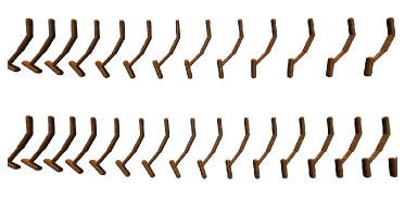
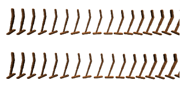
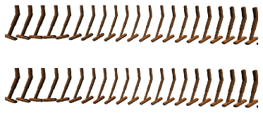
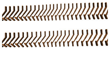
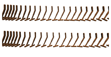
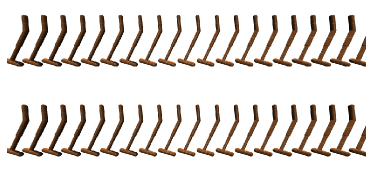
Figure F.1: Comparison of true state sequences and flow generated state sequences. In each panel, the top row plots a randomly sampled true state sequence from the hopper-medium dataset, and the bottom row plots the sequence sampled from the flow, conditioning on the first state and a large out-of-distribution RTG. The guidance weight is $3.0$.

F.2 Computational Speed Comparison

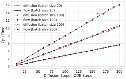
Figure F.2: The CPU time of generating a batch of $704$-dimensional vectors (The subsequence length is $64$, and each state is of dimension $11$), using different numbers of internal steps. The time consumed by the diffusion model and the flow are roughly the same.

References

- Ajay et al. (2022) Anurag Ajay, Yilun Du, Abhi Gupta, Joshua Tenenbaum, Tommi Jaakkola, and Pulkit Agrawal. Is conditional generative modeling all you need for decision-making? arXiv preprint arXiv:2211.15657, 2022.
- Akimov et al. (2022) Dmitriy Akimov, Vladislav Kurenkov, Alexander Nikulin, Denis Tarasov, and Sergey Kolesnikov. Let offline rl flow: Training conservative agents in the latent space of normalizing flows. arXiv preprint arXiv:2211.11096, 2022.
- Albergo and Vanden-Eijnden (2022) Michael S Albergo and Eric Vanden-Eijnden. Building normalizing flows with stochastic interpolants. arXiv preprint arXiv:2209.15571, 2022.
- Bellman (1957) Richard Bellman. A markovian decision process. Indiana Univ. Math. J., 1957.
- Brown et al. (2020) Tom B. Brown, Benjamin Mann, Nick Ryder, Melanie Subbiah, Jared Kaplan, Prafulla Dhariwal, Arvind Neelakantan, Pranav Shyam, Girish Sastry, Amanda Askell, Sandhini Agarwal, Ariel Herbert-Voss, Gretchen Krueger, Tom Henighan, Rewon Child, Aditya Ramesh, Daniel M. Ziegler, Jeffrey Wu, Clemens Winter, Christopher Hesse, Mark Chen, Eric Sigler, Mateusz Litwin, Scott Gray, Benjamin Chess, Jack Clark, Christopher Berner, Sam McCandlish, Alec Radford, Ilya Sutskever, and Dario Amodei. Language models are few-shot learners, 2020.
- Chen et al. (2021) Lili Chen, Kevin Lu, Aravind Rajeswaran, Kimin Lee, Aditya Grover, Michael Laskin, Pieter Abbeel, Aravind Srinivas, and Igor Mordatch. Decision transformer: Reinforcement learning via sequence modeling. In Thirty-Fifth Conference on Neural Information Processing Systems, 2021. URL https://openreview.net/forum?id=a7APmM4B9d.
- Chen et al. (2020a) Mark Chen, Alec Radford, Rewon Child, Jeffrey Wu, Heewoo Jun, David Luan, and Ilya Sutskever. Generative pretraining from pixels. In International conference on machine learning, pages 1691–1703. PMLR, 2020a.
- Chen et al. (2020b) Nanxin Chen, Yu Zhang, Heiga Zen, Ron J Weiss, Mohammad Norouzi, and William Chan. Wavegrad: Estimating gradients for waveform generation. arXiv preprint arXiv:2009.00713, 2020b.
- Chen et al. (2018) Ricky TQ Chen, Yulia Rubanova, Jesse Bettencourt, and David K Duvenaud. Neural ordinary differential equations. Advances in neural information processing systems, 31, 2018.
- Chi et al. (2023) Cheng Chi, Siyuan Feng, Yilun Du, Zhenjia Xu, Eric Cousineau, Benjamin Burchfiel, and Shuran Song. Diffusion policy: Visuomotor policy learning via action diffusion. arXiv preprint arXiv:2303.04137, 2023.
- Chrabaszcz et al. (2017) Patryk Chrabaszcz, Ilya Loshchilov, and Frank Hutter. A downsampled variant of imagenet as an alternative to the cifar datasets. arXiv preprint arXiv:1707.08819, 2017.
- Dao et al. (2023) Quan Dao, Hao Phung, Binh Nguyen, and Anh Tran. Flow matching in latent space. arXiv preprint arXiv:2307.08698, 2023.
- Dhariwal and Nichol (2021) Prafulla Dhariwal and Alexander Nichol. Diffusion models beat gans on image synthesis. Advances in neural information processing systems, 34:8780–8794, 2021.
- Emmons et al. (2021) Scott Emmons, Benjamin Eysenbach, Ilya Kostrikov, and Sergey Levine. Rvs: What is essential for offline rl via supervised learning? arXiv preprint arXiv:2112.10751, 2021.
- Fu et al. (2020) Justin Fu, Aviral Kumar, Ofir Nachum, George Tucker, and Sergey Levine. D4rl: Datasets for deep data-driven reinforcement learning. arXiv preprint arXiv:2004.07219, 2020.
- Ho and Salimans (2022) Jonathan Ho and Tim Salimans. Classifier-free diffusion guidance. arXiv preprint arXiv:2207.12598, 2022.
- Ho et al. (2020) Jonathan Ho, Ajay Jain, and Pieter Abbeel. Denoising diffusion probabilistic models. Advances in neural information processing systems, 33:6840–6851, 2020.
- Hu et al. (2023) Vincent Tao Hu, David W Zhang, Meng Tang, Pascal Mettes, Deli Zhao, and Cees GM Snoek. Latent space editing in transformer-based flow matching. In ICML Workshop on New Frontiers in Learning, Control, and Dynamical Systems, 2023.
- Janner et al. (2021) Michael Janner, Qiyang Li, and Sergey Levine. Offline reinforcement learning as one big sequence modeling problem. In Thirty-Fifth Conference on Neural Information Processing Systems, 2021. URL https://openreview.net/forum?id=wgeK563QgSw.
- Janner et al. (2022) Michael Janner, Yilun Du, Joshua B Tenenbaum, and Sergey Levine. Planning with diffusion for flexible behavior synthesis. arXiv preprint arXiv:2205.09991, 2022.
- Kawar et al. (2022) Bahjat Kawar, Michael Elad, Stefano Ermon, and Jiaming Song. Denoising diffusion restoration models. Advances in Neural Information Processing Systems, 35:23593–23606, 2022.
- Kingma and Ba (2014) Diederik P Kingma and Jimmy Ba. Adam: A method for stochastic optimization. arXiv preprint arXiv:1412.6980, 2014.
- Kingma et al. (2023) Diederik P. Kingma, Tim Salimans, Ben Poole, and Jonathan Ho. Variational diffusion models, 2023.
- Kober et al. (2013) Jens Kober, J Andrew Bagnell, and Jan Peters. Reinforcement learning in robotics: A survey. The International Journal of Robotics Research, 32(11):1238–1274, 2013.
- Kumar et al. (2019) Aviral Kumar, Xue Bin Peng, and Sergey Levine. Reward-conditioned policies. arXiv preprint arXiv:1912.13465, 2019.
- Le et al. (2023) Matthew Le, Apoorv Vyas, Bowen Shi, Brian Karrer, Leda Sari, Rashel Moritz, Mary Williamson, Vimal Manohar, Yossi Adi, Jay Mahadeokar, et al. Voicebox: Text-guided multilingual universal speech generation at scale. Advances in neural information processing systems, 2023.
- Lee et al. (2022) Kuang-Huei Lee, Ofir Nachum, Mengjiao Sherry Yang, Lisa Lee, Daniel Freeman, Sergio Guadarrama, Ian Fischer, Winnie Xu, Eric Jang, Henryk Michalewski, et al. Multi-game decision transformers. Advances in Neural Information Processing Systems, 35:27921–27936, 2022.
- Levine et al. (2020) Sergey Levine, Aviral Kumar, George Tucker, and Justin Fu. Offline reinforcement learning: Tutorial, review, and perspectives on open problems. arXiv preprint arXiv:2005.01643, 2020.
- Li et al. (2016) Jiwei Li, Will Monroe, Alan Ritter, Michel Galley, Jianfeng Gao, and Dan Jurafsky. Deep reinforcement learning for dialogue generation. arXiv preprint arXiv:1606.01541, 2016.
- Lin et al. (2023) Shanchuan Lin, Bingchen Liu, Jiashi Li, and Xiao Yang. Common diffusion noise schedules and sample steps are flawed. arXiv preprint arXiv:2305.08891, 2023.
- Lipman et al. (2023) Yaron Lipman, Ricky T. Q. Chen, Heli Ben-Hamu, Maximilian Nickel, and Matt Le. Flow matching for generative modeling. International Conference on Learning Representations, 2023.
- Lu et al. (2022) Kevin Lu, Aditya Grover, Pieter Abbeel, and Igor Mordatch. Pretrained transformers as universal computation engines. In Proceedings of the AAAI Conference on Artificial Intelligence, 2022.
- Mish (2019) Misra D Mish. A self regularized non-monotonic activation function [j]. arXiv preprint arXiv:1908.08681, 2019.
- Nguyen et al. (2022) T Nguyen, Q Zheng, and A Grover. Reliable conditioning of behavioral cloning for offline reinforcement learning. arXiv preprint arXiv:2210.05158, 2022.
- Nichol and Dhariwal (2021) Alexander Quinn Nichol and Prafulla Dhariwal. Improved denoising diffusion probabilistic models. In International Conference on Machine Learning, pages 8162–8171. PMLR, 2021.
- Pokle et al. (2023) Ashwini Pokle, Matthew J Muckley, Ricky TQ Chen, and Brian Karrer. Training-free linear image inversion via flows. arXiv preprint arXiv:2310.04432, 2023.
- Pooladian et al. (2023) Aram-Alexandre Pooladian, Heli Ben-Hamu, Carles Domingo-Enrich, Brandon Amos, Yaron Lipman, and Ricky Chen. Multisample flow matching: Straightening flows with minibatch couplings. arXiv preprint arXiv:2304.14772, 2023.
- Radford et al. (2018) Alec Radford, Karthik Narasimhan, Tim Salimans, and Ilya Sutskever. Improving language understanding by generative pre-training. 2018.
- Reed et al. (2022) Scott Reed, Konrad Zolna, Emilio Parisotto, Sergio Gomez Colmenarejo, Alexander Novikov, Gabriel Barth-Maron, Mai Gimenez, Yury Sulsky, Jackie Kay, Jost Tobias Springenberg, et al. A generalist agent. arXiv preprint arXiv:2205.06175, 2022.
- Rombach et al. (2022) Robin Rombach, Andreas Blattmann, Dominik Lorenz, Patrick Esser, and Björn Ommer. High-resolution image synthesis with latent diffusion models. In Proceedings of the IEEE/CVF conference on computer vision and pattern recognition, pages 10684–10695, 2022.
- Salimans and Ho (2022) Tim Salimans and Jonathan Ho. Progressive distillation for fast sampling of diffusion models. arXiv preprint arXiv:2202.00512, 2022.
- Schmidhuber (2019) Juergen Schmidhuber. Reinforcement learning upside down: Don’t predict rewards–just map them to actions. arXiv preprint arXiv:1912.02875, 2019.
- Silver et al. (2016) David Silver, Aja Huang, Chris J Maddison, Arthur Guez, Laurent Sifre, George Van Den Driessche, Julian Schrittwieser, Ioannis Antonoglou, Veda Panneershelvam, Marc Lanctot, et al. Mastering the game of go with deep neural networks and tree search. nature, 529(7587):484–489, 2016.
- Singh et al. (1999) Satinder Singh, Michael Kearns, Diane Litman, and Marilyn Walker. Reinforcement learning for spoken dialogue systems. Advances in neural information processing systems, 12, 1999.
- Sohl-Dickstein et al. (2015) Jascha Sohl-Dickstein, Eric Weiss, Niru Maheswaranathan, and Surya Ganguli. Deep unsupervised learning using nonequilibrium thermodynamics. In International conference on machine learning, pages 2256–2265. PMLR, 2015.
- Song et al. (2020a) Jiaming Song, Chenlin Meng, and Stefano Ermon. Denoising diffusion implicit models. arXiv preprint arXiv:2010.02502, 2020a.
- Song et al. (2020b) Yang Song, Jascha Sohl-Dickstein, Diederik P Kingma, Abhishek Kumar, Stefano Ermon, and Ben Poole. Score-based generative modeling through stochastic differential equations. arXiv preprint arXiv:2011.13456, 2020b.
- Srivastava et al. (2019) Rupesh Kumar Srivastava, Pranav Shyam, Filipe Mutz, Wojciech Jaśkowski, and Jürgen Schmidhuber. Training agents using upside-down reinforcement learning. arXiv preprint arXiv:1912.02877, 2019.
- Vaswani et al. (2017) Ashish Vaswani, Noam Shazeer, Niki Parmar, Jakob Uszkoreit, Llion Jones, Aidan N Gomez, Łukasz Kaiser, and Illia Polosukhin. Attention is all you need. In Advances in neural information processing systems, pages 5998–6008, 2017.
- Wang et al. (2023) Chengyi Wang, Sanyuan Chen, Yu Wu, Ziqiang Zhang, Long Zhou, Shujie Liu, Zhuo Chen, Yanqing Liu, Huaming Wang, Jinyu Li, et al. Neural codec language models are zero-shot text to speech synthesizers. arXiv preprint arXiv:2301.02111, 2023.
- Wang et al. (2018) Yuxuan Wang, Daisy Stanton, Yu Zhang, RJ-Skerry Ryan, Eric Battenberg, Joel Shor, Ying Xiao, Ye Jia, Fei Ren, and Rif A Saurous. Style tokens: Unsupervised style modeling, control and transfer in end-to-end speech synthesis. In International conference on machine learning, pages 5180–5189. PMLR, 2018.
- Wang et al. (2022) Zhendong Wang, Jonathan J Hunt, and Mingyuan Zhou. Diffusion policies as an expressive policy class for offline reinforcement learning. arXiv preprint arXiv:2208.06193, 2022.
- Ward et al. (2019) Patrick Nadeem Ward, Ariella Smofsky, and Avishek Joey Bose. Improving exploration in soft-actor-critic with normalizing flows policies. arXiv preprint arXiv:1906.02771, 2019.
- Wu and He (2018) Yuxin Wu and Kaiming He. Group normalization. In Proceedings of the European conference on computer vision (ECCV), pages 3–19, 2018.
- Zhao and Grover (2023) Siyan Zhao and Aditya Grover. Decision stacks: Flexible reinforcement learning via modular generative models. arXiv preprint arXiv:2306.06253, 2023.
- Zheng et al. (2022) Qinqing Zheng, Amy Zhang, and Aditya Grover. Online decision transformer. In international conference on machine learning, pages 27042–27059. PMLR, 2022.
- Zheng et al. (2023) Qinqing Zheng, Mikael Henaff, Brandon Amos, and Aditya Grover. Semi-supervised offline reinforcement learning with action-free trajectories. In International conference on machine learning, pages 42339–42362. PMLR, 2023.