New efficient ADMM algorithm for the Unit Commitment Problem

Abstract

The unit commitment problem (UC) is an optimization problem concerning the operation of electrical generators. Many algorithms have been proposed for the UC and in recent years a more decentralized approach, by solving the UC with alternating direction method of multipliers (ADMM), has been investigated. For convex problems ADMM is guaranteed to find an optimal solution. However, because UC is non-convex additional steps need to be taken in order to ensure convergence to a feasible solution of high quality. Therefore, solving UC by a MIL(Q)P formulation and running an off-the-shelf solver like Gurobi until now seems to be the most efficient approach to obtain high quality solutions.

In this paper, we introduce a new and efficient way to solve the UC with ADMM to near optimality. We relax the supply-demand balance constraint and deal with the non-convexity by iteratively increasing a penalty coefficient until we eventually force convergence and feasibility. At each iteration the subproblems are solved by our efficient algorithm for the single UC subproblem developed in earlier work and our new ADMM algorithm for the transmission subproblems.

Computational experiments on benchmark instances demonstrated that our algorithm produces high-quality solutions. The computation time seems to grow practically linear with the length of the time horizon. For the case with quadratic generation cost our algorithm is significantly faster than solving the problem by a state-of-the-art MIL(Q)P formulation. For the case of linear generation cost, it outperforms the MILP approach for longer time horizons.

1 Introduction

The unit commitment problem (UC) is a family of NP-hard van Ackooij et al. [2018], Melhorn et al. [2016] optimization problems for the operational planning of electrical generators. The goal is to find a minimum cost schedule of generators that satisfies the electricity demand at each time step. UC is a widely studied topic in Operations Research, but its significance extends beyond this field, as it plays a central role in detailed power system modeling, which is crucial in the ongoing global shift towards sustainable energy Welsch et al. [2014], Abujarad et al. [2017].

The UC has been extensively researched in academia, with various optimization techniques applied to solve it. This can be seen in the numerous papers cited in various surveys on the topic van Ackooij et al. [2018], Saravanan et al. [2013], Padhy [2004] spanning multiple algorithm paradigms, from exact methods to heuristic evolutionary algorithms. However, since UC has a mixed combinatorial and continuous statespace, mathematical programming techniques have been most successful in finding near optimal solutions van Ackooij et al. [2018]. Until the early 2000’s, Lagrangian Relaxation was the method of choice for solving UC Borghetti et al. [2003]. However, this has changed. In the past 15 years, Mixed Integer Linear Programming (MILP) problem formulations have been a very active area of research Knueven et al. [2020] and popular tool for solving the UC Atakan et al. [2017], Taktak and D’Ambrosio [2017], Morales-España et al. [2013]. Additionally, it has been stated that in the industry, UC is commonly solved using MILP and that the shift from Lagrangian Relaxation to MILP was considered beneficial O’Neill et al. [2011], Carlson et al. [2012], O’Neill [2007].

The recent resurgence of interest in alternating direction method of multipliers (ADMM) Yang et al. [2022] have also resulted in an increased application of augmented Lagrangian methods, such as ADMM, to the UC Feizollahi et al. [2015], Kraning et al. [2014], Ramanan et al. [2017], Zhang and Hedman [2021], Xavier et al. [2020].

ADMM is an augmented Lagrangian method that solves convex optimization problems. In ADMM, decision variables are split into two or more subsets, and the coupling constraints, i.e constraints involving variables from different subsets, are relaxed by moving them to the objective such that violation of these constraints results in a penalty cost. Next, at consecutive steps subproblems are solved over a subset of the variables. These subproblems are much easier to solve than the original problem and this can be done in a distributed and parallel way.

The UC problem can be decomposed in multiple ways. For example, ADMM can be applied to the UC by relaxing the demand coupling constraint at each node, which was done by Kraning et al. [2014] and is also commonly used in existing literature on Lagrangian relaxation for UC Borghetti et al. [2001], Fan et al. [2002a], Frangioni et al. [2008]. The demand coupling constraint at a node ensures that the total production of electricity is equal to the consumption of electricity. By relaxing this constraint, the problem decomposes into multiple subproblems for the generators, Renewable Energy Sources (RES), transmission, and storage units. These subproblems can then be solved by efficient algorithms Wuijts et al. [2021a], Frangioni and Gentile [2006], Guan et al. [2003], Fan et al. [2002b]. The Lagrange multipliers at each node corresponds to a nodal electricity price for each time step.

When the problem is decomposed at the transmission level Feizollahi et al. [2015], Ramanan et al. [2017], Xavier et al. [2020], Zhang and Hedman [2021], the nodes of the power system are divided into regions, which are then decoupled by copying transmission variables at their boundaries and relaxing the equality between these copied variables. If you decompose at the transmission level, the subproblems at each node are (smaller) UC problems which contain a subset of the total generators, RES and storage units. These UC problems can still be hard to solve and are often solved with MILP.

There are several other possible decompositions. For example, duplicated dispatch variables can be used in different subproblems of the UC problem Batut and Renaud [1992] or temporal constraints such as ramping limits or minimum up- and downtime can be relaxed Safdarian et al. [2019].

Only for convex optimization problems, ADMM is guaranteed to find an optimal solution Boyd et al. [2011]. However, since UC is non-convex due to the binary commitment variables, researchers using ADMM to solve UC must be aware that it may not converge to the optimal solution, if at all. This is a general drawback of decomposition algorithms based on Lagrangian relaxation.

Some authors Feizollahi et al. [2015], Xavier et al. [2020] solved the issue of nonconvexity by embedding their ADMM algorithm into a larger heuristic that after some iterations fixes the binary commitment variables to make the problem convex. The ADMM algorithm can then converge towards the local optimal solution given these fixed binary variables. This process is called “release-and-fix”. It is not guaranteed that these fixed commitment variables are optimal or even result in feasible solutions.

Another approach is to repair the final solution provided by Lagrangian relaxation in an ad hoc way by fixing the binary variables with some heuristic Feltenmark [1997], Yan et al. [1993], Borghetti et al. [2003], Frangioni et al. [2008]. A convex economic dispatch problem is then solved with these fixed binary variables. For example, the heuristics proposed by Feltenmark [1997] sequentially and greedily processes the timesteps, fixing binary variables while adhering to minimum up times. Which generators are being turned on or off is based on either a priority list or randomly sampled from a probability distribution calculated using information from their bundle methods. They introduce four variants, one of which is deterministic and the others use sampling. When sampling is used, the heuristics are repeated, and the best solution is retained. The authors found that three out of the four proposed heuristics frequently fail to produce feasible solution and the fourth one requires a lot of sampling steps (repeated 200 Feltenmark and Kiwiel [2000] or 1000 Feltenmark [1997] times).

Note that in the above heuristics ramping limits are ignored. Frangioni et al. [2008] and Borghetti et al. [2003] both use a slight modification of one of the four heuristics proposed Feltenmark [1997]. Frangioni et al. [2008] studies the case of UC with ramping limits and only finds feasible solutions in roughly one out of ten dual iterations. Moreover, the authors state that incorporating ramping limits into their heuristic is non-trivial.

Other authors try to force feasibility by adding an additional penalty function Dubost et al. [2005]. However, solutions produced are still infeasible and far away from optimality. Finally, others have chosen to just ignore the issue Batut and Renaud [1992] and some authors chose to convexify the generator polytope, i.e. they remove the non-convexity by taking the convex-hull of the generator state space Kraning et al. [2014], again leading to infeasible solutions.

Our contribution: in this paper we introduce a new and efficient way to solve UC with ADMM. We relax the demand coupling constraint and improve existing approaches in two ways. Firstly, we apply a different method to deal with the non-convexity by using an increasing penalty coefficient. This means that we do not need heuristic approaches to transfer the infeasible solution into a feasible one. Our algorithm is the first Langrangian algorithm to force convergence and feasibility for the UC including ramping limits without requiring an ad-hoc repair heuristic. Secondly, we solve the subproblems very efficiently by applying our 1UC algorithm Wuijts et al. [2021a], which strongly outperforms earlier algorithms for 1UC especially on longer time horizons, and also our newly created algorithm to solve transmission sub problems. We performed computational experiments on all known benchmark instances. Although our ADMM algorithm needs many iterations to converge, each iteration has a low computation time due to our efficient 1UC algorithm.

Consequently, we have introduced a fast algorithm that produces high quality solutions respecting the ramping limits which experimentally outperforms solving UC with MIP formulations, the current state-of-the-art for the UC. Moreover, our method scales much better with the length of the planning horizon. In the experiments, we always found feasible solutions of a very good quality for a large set of UC instances.

The remainder of this paper is organized as follows. In the following section, we present the problem formulation of UC. In Section 3, we describe how ADMM can be applied to a small power system. In Section 4, we describe how we applied ADMM to a full UC formulation, how we solve the individual subproblems and how we dealt with non-convexity. Our experiments and results are presented in Section 5, and we end the paper with a discussion in Section 6 and conclusions in Section 7.

2 UC problem description

In this section, we define the UC that we study in this paper. Our UC description is based on a Mixed Integer Quadratic Program (MIQP) formulation with detailed thermal generators, RES, storage, and transmission lines. The decision variables $p_{gt}$, $p_{rt}$, $p_{st}$ are the generation of thermal generator unit $g$, RES unit $s$ and storage unit $s$ at time step $t$. Other variables are created to specify the feasible state space of these variables. We use the well-known 3-bin formulation Knueven et al. [2020]. This means that we use binary variables $u_{gt}$, $v_{gt}$, and $w_{gt}$ to signal that generator $g$ respectively is on, switched on, and switched off in time step $t$ . The formulation is as follows:

$$\min\sum_{t\in T}\sum_{g\in G}a_{g}u_{gt}+b_{g}p_{gt}+c_{g}p_{gt}^{2}+v_{gt}cost_{start}$$ (1a)

$$s.t.$$

$$p_{gt}\geq u_{gt}\underline{P}_{g},g\in G,t\in T$$ (1b)

$$p_{gt}\leq\overline{P}_{g}u_{gt},g\in G,t\in T$$ (1c)

$$\sum_{i=t-UT_{g}+1}^{t}v_{gi}\leq u_{gt},t\in T,g\in G$$ (1d)

$$\sum_{i=t-DT_{g}+1}^{t}w_{gi}\leq 1-u_{gt},t\in T,g\in G$$ (1e)

$$p_{gt}-p_{gt-1}\leq(SU_{g}-RU_{g})v_{gt}+RU_{g}u_{gt},t\geq 2,g\in G$$ (1f)

$$p_{gt-1}-p_{gt}\leq(SD_{g}-RD_{g})w_{gt}+RD_{g}u_{gt-1},t\geq 2,g\in G$$ (1g)

$$p_{rt}\leq AF_{rt}\overline{P}_{rt},r\in R,t\in T$$ (1h)

$$0\leq pc_{st}\leq\overline{PC}_{s},t\in T,s\in S$$ (1i)

$$0\leq pd_{st}\leq\overline{PD}_{s},t\in T,s\in S$$ (1j)

$$p_{st}=pd_{st}-pc_{st},t\in T,s\in S$$ (1k)

$$\underline{PE}_{s}\leq pe_{st}\leq\overline{PE}_{s},t\in T,s\in S$$ (1l)

$$pe_{st}=pe_{st-1}+pc_{st}*\eta^{c}_{st}-\frac{pd_{st}}{\eta^{d}_{st}},t\in T,s\in S$$ (1m)

$$inj_{nt}=\sum_{l=(n^{\prime}\rightarrow n),n^{\prime}\in N}f_{lt},t\in T,n\in N$$ (1n)

$$\underline{f_{l}}\leq f_{lt}\leq\overline{f_{l}},l\in L,t\in T$$ (1o)

$$\sum_{g\in G_{n}}p_{gt}+\sum_{r\in R_{n}}p_{rt}+\sum_{s\in S_{n}}p_{st}+inj_{nt}=D_{nt},t\in T,n\in N$$ (1p)

$$u_{gt}-u_{gt-1}=v_{gt}-w_{gt},t\in T,g\in G$$ (1q)

$$u_{gt},v_{gt},w_{gt}\in\{0,1\},p_{gt},p_{rt},p_{st},pe_{st},inj_{nt},f_{lt}\in\mathbb{R}$$ (1r)

(1a) is the objective function of the UC consisting of the generation cost and start cost, $a_{g}$ is the constant cost, $b_{g}$ is the linear cost coefficient and $c_{g}$ is the quadratic cost coefficient. Constraint (1b) and (1c) ensure the minimum and maximum production of generators. Constraint (1d) and (1e) ensure the minimum up and downtime of generators. Constraint (1f) and (1g) ensure the ramping limits of generators between time steps. Constraint (1h) ensures that the RES production is lower than the availability at that hour. (1i), (1j) and (1l) ensure the charge, discharge and energy storage limits for storage units. Equation (1k) is the sum of charge and discharge i.e. the net storage production. Equation (1m) describes the relation between the charge, discharge and net power production of a storage unit. Equation (1q) describes the logic between the binary commitment, start and stop variables of the generators. Equation (1n) describes the relation between the flow on transmission lines and the power injection at nodes. Constraint (1o) ensures flow limits on transmission lines. Equation (1p) ensures that the total generation meets the total demand at every node and time step. At last, the commitment variables are binary while the generation are real numbers (1r)

3 ADMM Example on simple UC problem

To illustrate the application of ADMM to UC, we present here a simple UC example. Suppose we want to find the least cost power production schedule for a power system with a demand $D$ and $n$ generators with generation levels $p_{i}$ and a convex generation cost function $f_{i}$ for generator $i$. This optimization problem can be formulated as:

$$\min\sum_{1\leq i\leq n}f_{i}(p_{i})$$ (2)

$$s.t.$$

$$D-\sum_{1\leq i\leq n}p_{i}=0$$ (3)

We can solve this problem by first taking the augmented Lagrange relaxation of the demand coupling constraint (3) and for a giving $\rho$ turning it in the following function:

$$\mathcal{L}(p_{1},\dots,p_{n},\lambda)=\sum_{1\leq i\leq n}f_{i}(p_{i})+\lambda(D-\sum_{1\leq i\leq n}p_{i})+\frac{\rho}{2}(D-\sum_{1\leq i\leq n}p_{i})^{2}$$ (4)

we can define the corresponding dual problem as:

$$\max_{\lambda}g(\lambda)$$ (5)

$$\text{where }g(\lambda)=\inf_{\mathbf{p}}\mathcal{L}(\mathbf{p},\lambda)$$

If strong duality holds, the optimal value of the dual problem (5) is the same as the optimal value of the primal problem (2). Then the optimal primal solution can be recovered from the optimal dual solution. We can find the optimal multiplier $\lambda$ by doing dual descent, i.e. iteratively solving $\inf_{\mathbf{p}}\mathcal{L}(\mathbf{p},\lambda)$ for a given $\lambda$ and update $\lambda$ in the direction of the gradient of $g$ (5).

However, contrary to solving a standard Lagrangian iteration, we cannot determine the optimal generation $p_{i}$ independently of the other production variables when solving an augmented Lagrangian iteration. Unfortunately, this makes the augmented Lagrangian dual iteration as difficult as solving the original primal problem.

A solution to deal with the interdependence of the subproblems is ADMM. The idea of ADMM is that you iteratively optimize one subproblem while the other subproblems stay fixed. In other words, only a subset of the decision variables can change while the rest of the decision variables remain fixed at the value of the previous iteration or, if they have already been updated, of the current iteration. At the end of the ADMM iteration the dual multipliers are updated (see Boyd et al. [2011] for a detailed explanation of ADMM).

When the original problem is convex and the problem is split into two sets of variables then this method will converge to a primal feasible solution with an optimal value Boyd et al. [2011]. However, a lot of optimization problems have a decomposable structure that consist of multiple sets or blocks. To decompose a problem that has a multi-block structure we can either use multi-block Gauss Seidel ADMM or variable splitting ADMM which at its core has a two-block structure Liu and Han [2015]. The former ADMM method has been applied to practical problems Liu and Han [2015] but lacks the converging guaranty of the latter Chen et al. [2016].

3.1 Multi-block Gauss Seidel

We apply Gauss Seidel ADMM to determine the optimal Lagrange multipliers and generation for the UC example. At each iteration $k$ we sequentially minimize $p_{i}$ while keeping the other production values constant. The values $p_{j}^{k+1}$ are used for generators $j$ where $j<i$ and for generators $j>i$ we use the old value $p_{j}^{k}$ of the previous iteration, resulting in each iteration in $n$ statements of the form:

$$p_{i}^{k+1}\leftarrow\text{argmin}_{p_{i}}\mathcal{L}(p_{1}^{k+1},\dots,p_{i-1}^{k+1},p_{i},p_{i+1}^{k},\dots,p_{n}^{k},\lambda^{k})$$ (6)

The strength of ADMM is that we remove the interdependence created by the cross term in (4) by optimizing only for $p_{i}$ while keeping the other values constant.

At the end of each iteration, the multiplier is updated in the direction of the gradient of the relaxed constraint violation with step size $\rho$. For readability, we define the relevant residual load $R_{i}$ for generator $i$:

$$R_{i}=D-\sum_{1\leq j<i}p_{j}^{k+1}-\sum_{i<j\leq n}p_{j}^{k}$$ (7)

The full Gauss-Seidel multi-block ADMM that solves our small UC example with $n$ generators is presented in Algorithm 1.

while Stopping criteria have not been met do

     $p_{1}^{k+1}\leftarrow\text{argmin}_{p_{1}}\{f_{1}(p_{1})-\lambda^{k}p_{1}+\frac{\rho}{2}(R_{1}-p_{1})^{2}\}$ $\triangleright$ $\text{argmin}_{p_{1}}\mathcal{L}(p_{1},\dots,p_{n}^{k},\lambda)$

     $\vdots$

     $p_{i}^{k+1}\leftarrow\text{argmin}_{p_{i}}\{f_{i}(p_{i})-\lambda^{k}p_{i}+\frac{\rho}{2}(R_{i}-p_{i})^{2}\}$ $\triangleright$ $\text{argmin}_{p_{i}}\mathcal{L}(p_{1}^{k+1}\dots p_{i}\dots p_{n}^{k},\lambda)$

     $\vdots$

     $p_{n}^{k+1}\leftarrow\text{argmin}_{p_{n}}\{f_{n}(p_{n})-\lambda^{k}p_{n}+\frac{\rho}{2}(R_{n}-p_{n})^{2}\}$ $\triangleright$ $\text{argmin}_{p_{n}}\mathcal{L}(p_{1}^{k+1},\dots,p_{n},\lambda)$

     $\lambda^{k+1}\leftarrow\lambda^{k}+\rho(D-\sum_{1\leq i\leq n}p_{i}^{k+1})$

     $k\leftarrow k+1$

end while

Algorithm 1 Gauss-Seidel Multi-block ADMM

An alternative method of applying ADMM on a problem with a multi-block structure is by variable splitting, but we found that this ADMM performed much worse than the Gauss Seidel ADMM. More information is presented in the appendix.

4 New ADMM Algorithm for UC

After the application of ADMM to a simple UC example, we now apply ADMM to the full UC problem described in Section 2. Although the procedure is also based on the relaxation of the coupling constraint that links generation and demand, the individual subproblems are more complicated.

In the UC description (1a) - (1r) the only constraint that links the generation and demand is (1p). We obtain the following augmented Lagrangian by relaxing this constraint:

$$\mathcal{L}(\overrightarrow{p_{gt}},\overrightarrow{p_{rt}},\overrightarrow{p_{st}},\overrightarrow{inj_{nt}},\overrightarrow{\lambda_{nt}})=\sum_{t\in T}\sum_{g\in G}\left[a_{g}+b_{g}p_{gt}+c_{g}p_{gt}^{2}+v_{gt}cost_{start}\right]+$$

$$\sum_{t\in T}\sum_{n\in N}\left[\lambda_{nt}RD_{nt}+\frac{\rho}{2}RD_{nt}^{2}\right]$$ (8a)

$$\text{s.t. }(\ref{eq:chapter3:pmin})-(\ref{eq:chapter3:trans3})$$ (8b)

where:

$$RD_{nt} =D_{nt}-(\sum_{g\in G_{n}}p_{gt}+\sum_{r\in R_{n}}p_{rt}+\sum_{s\in S_{n}}p_{st}+inj_{nt})$$

$\lambda_{nt}$ is the Lagrange multiplier of coupling constraint of node $n$ at time $t$ and $\rho$ is the quadratic penalty coefficient on the residual demand.

At each iteration the optimal value of the decision variables will be determined while the rest of the decision variables remain fixed at the value of the previous iteration or, if they have already been updated, of the current iteration. Consequently, we iteratively solve the following subproblems: single unit commitment subproblem (1UC) for each generator $g\in G$, RES subproblem for each renewable resource $r\in R$, storage subproblem for each storage unit $s\in S$, and the transmission subproblem for each time step $t\in T$. This is depicted in (Figure 1).

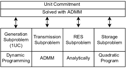
Figure 1: Flowchart of solving UC with ADMM by decomposing it into subproblems.

After each iteration the Lagrange multipliers are updated in the direction of the sub-gradient which equals to the residual demand $RD_{nt}$. The ADMM Gauss-Seidel iteration proceeds according to Algorithm 2.

Algorithm 2 Gauss-Seidel ADMM iteration

for all $g\in G$ do

     $\mathbf{p}_{g}\leftarrow\text{argmin}_{p_{g}}\mathcal{L}(\dots,p_{g-1}^{k+1},p_{g},p_{g+1}^{k}\dots,\lambda^{k})$ $\triangleright$ Solve 1UC subproblem

end for

for all $r\in R$ do

     $\mathbf{p}_{r}\leftarrow\text{argmin}_{p_{r}}\mathcal{L}(\dots,p_{r-1}^{k+1},p_{r},p_{r+1}^{k}\dots,\lambda^{k})$ $\triangleright$ Solve 1RES subproblem

end for

for all $s\in S$ do

     $p_{s}\leftarrow\text{argmin}_{p_{s}}\mathcal{L}(\dots,p_{s-1}^{k+1}p_{s},p_{s+1}^{k}\dots,\lambda^{k})$ $\triangleright$ Solve 1Storage subproblem

end for

for all $t\in T$ do

     $\mathbf{inj}_{t}\leftarrow\text{argmin}_{inj_{t}}\mathcal{L}(\dots,inj_{t},\dots,\lambda^{k})$ $\triangleright$ Solve Transmission subproblem

end for

for all $t\in T$ do

     for all $n\in N$ do

         $\lambda_{nt}^{k+1}\leftarrow\lambda_{nt}^{k}+\rho RD_{nt}^{k}$ $\triangleright$ Update Lagrangian multipliers

     end for

end for

4.1 Solving the subproblems

4.1.1 Generator subproblem 1UC

The 1UC problem is the problem of determining the optimal power schedule for a single generator. In each iteration of our Gauss-Seidel algorithm, we have to solve a number of 1UC problems (see Line 2 in Algorithm 2). For a given generator $g$ at node $n$, this problem can be defined as:

$$\text{argmin}_{p_{g}}\mathcal{L}(\dots,p_{g-1}^{k+1},p_{g},p_{g+1}^{k}\dots,\lambda^{k})\text{ s.t. }(\ref{eq:chapter3:pmin})-(\ref{eq:chapter3:domain})$$ (9)

Only $p_{g}$ is variable here, the other production variables $p_{g}$ $(g\in G_{n})$ are constant.

Similar to the the small UC example in Section 3.1, we define the relevant residual load $R_{gnt}$ for determining the optimal power output of generator $g$ at node $n$ and time $t$ by

$$R_{gnt}=D_{nt}-\sum_{1\leq i<g}p_{it}^{k+1}-\sum_{g<i\leq\mid G_{n}\mid}p_{it}^{k}-\sum_{r\in R_{n}}p_{rt}^{k}-\sum_{s\in S_{n}}p_{st}^{k}-inj_{nt}^{k}$$ (10)

We can rewrite (9) to an equivalent problem formulation:

$$\min\sum_{t\in T}a_{g}+b_{g}p_{gt}+c_{g}p_{gt}^{2}+v_{gt}cost_{start}-\lambda_{t}p_{gt}+\frac{\rho}{2}(R_{gnt}-p_{gt})^{2}$$ (11)

$$\text{subject to }(\ref{eq:chapter3:pmin}),(\ref{eq:chapter3:pmax}),(\ref{eq:chapter3:MDT1}),(\ref{eq:chapter3:MDT2}),(\ref{eq:chapter3:logic}),(\ref{eq:chapter3:tightRamp1}),(\ref{eq:chapter3:tightRamp2})$$ (12)

Solving 1UC.

Since we have to solve a series of 1UC problems in each iteration, solving these problems very efficiently is crucial. Here we use our dynamic programming algorithm $RRF+$ Wuijts et al. [2021a], which significantly outperforms earlier 1UC algorithms in terms of computation time. This advanced dynamic programming algorithm models part of the states by convex functions instead of single values. This algorithm is based on a recurrence relation on functions that represents for each generator state at each time step the value of the optimal generator schedule that ends in that state. The RFF+ algorithm is very efficient because it does not need to compute the optimal economic dispatch for each possible ‘on-interval’ of a generator and it can identify superfluous functions which reduces the computation time significantly (see Wuijts et al. [2021a] for more details).

4.1.2 Renewable generation subproblem 1RES

The 1RES subproblem is the problem of finding the optimal renewable energy generation given its availability and is given by:

$$\text{argmin}_{p_{r}}\mathcal{L}(\dots,p_{r-1}^{k+1},p_{r},p_{r+1}^{k}\dots,\lambda^{k}) \text{ s.t. }(\ref{eq:chapter3:pmin})-(\ref{eq:chapter3:domain})$$ (13)

We define the relevant residual load $R_{rnt}$ for RES $r$ at node $n$ and time $t$.

$$R_{rnt}=D_{nt}-\sum_{g\in G_{n}}p_{gt}^{k+1}-\sum_{1\leq i<r}p_{rt}^{k+1}-\sum_{r<i\leq\mid R_{n}\mid}p_{rt}^{k}-\sum_{s\in S_{n}}p_{st}^{k}-inj_{nt}^{k}$$ (14)

Now (13) is equivalent to the following program:

$$\min\sum_{t\in T}-\lambda_{t}^{k}p_{rt}+\frac{\rho}{2}(R_{rnt}-p_{rt})^{2}$$ (15)

$$\text{subject to }p_{rt}\leq AF_{rt}\overline{P}_{rt} t\in T$$ (16)

We can easily solve this problem analytically since it is a simple minimization of a quadratic function with bounds, which results in:

$$p^{k+1}_{rt}=\begin{cases}0&\frac{\lambda^{k}_{t}}{R_{rnt}}<0\\ \frac{\lambda^{k}_{t}}{R_{rnt}}&0\leq\frac{\lambda^{k}_{t}}{R_{rnt}}\leq AF_{rt}\overline{P}_{rt}\\ AF_{rt}\overline{P}_{rt}&\frac{\lambda^{k}_{t}}{R_{rnt}}>AF_{rt}\overline{P}_{rt}\\ \end{cases}$$ (17)

4.1.3 Storage subproblem 1Storage

The storage subproblem to find the least cost charging and discharging strategy is given by:

$$\text{argmin}_{p_{s}}\mathcal{L}(\dots,p_{s-1}^{k+1},p_{s},p_{s+1}^{k}\dots,\lambda^{k}) \text{ s.t. }(\ref{eq:chapter3:pmin})-(\ref{eq:chapter3:domain})$$ (18)

We define the relevant residual load $R_{snt}$ for storage unit $s$ at node $n$ and time $t$.

$$R_{snt}=D_{nt}-\sum_{g\in G_{n}}p_{gt}^{k+1}-\sum_{r\in R_{n}}p_{rt}^{k+1}-\sum_{1\leq i<s}p_{st}^{k+1}-\sum_{s<i\leq\mid S_{n}\mid}p_{st}^{k}-inj_{nt}^{k}$$ (19)

To find the best storage schedule (18), we can simply solve the following quadratic program:

$$\min\sum_{t\in T}-\lambda^{k}_{t}p_{st}+\frac{\rho}{2}(R_{snt}-p_{st})^{2}$$ (20)

$$\text{subject to }(\ref{eq:chapter3:EnergyLimit}),(\ref{eq:chapter3:ChargeLimit}),(\ref{eq:chapter3:DischargeLimit}),(\ref{eq:chapter3:NetStorageProduction}),(\ref{eq:chapter3:StorageProduction})$$ (21)

Although other algorithms exist that solve this problem efficiently with dynamic programming Bannister and Kaye [1991], we solve this storage subproblem with the QP-solver Gurobi.

4.1.4 Transmission subproblem

The transmission subproblem is given by

$$\text{argmin}_{inj_{nt}}\mathcal{L}(\dots,inj_{nt},\dots,\lambda^{k}) \text{ s.t. }(\ref{eq:chapter3:pmin})-(\ref{eq:chapter3:domain})$$ (22)

The transmission subproblem (22) is harder than the RES or storage subproblems but fortunately it consists of a set of the subproblems which are independent in time. We define the relevant residual load $R_{nt}$ for the optimal nodal injection at node $n$ and time $t$.

$$R_{nt}=D_{nt}-\sum_{g\in G_{n}}p_{gt}^{k+1}-\sum_{r\in R_{n}}p_{rt}^{k+1}-\sum_{s\in S_{n}}p_{st}^{k+1}$$ (23)

Moreover, we define a set $L_{n}$ as $\{l\mid l\in L,n^{\prime}\in N,l=(n^{\prime}\rightarrow n)\}$ i.e. the set of transmission line going into $n$. For each time step $t\in T$ we have to solve the transmission subproblem that is equivalent to (22):

$$\min\sum_{n\in N}-\lambda^{k}_{n}inj_{n}+\frac{\rho}{2}(R_{nt}-inj_{n})^{2}$$ (24a)

subject to

$$inj_{n}=\sum_{l\in L_{n}}f_{l} \forall n\in N$$ (24b)

$$\underline{f_{l}}\leq f_{l}\leq\overline{f_{l}} \forall l\in L$$ (24c)

This subproblem is a quadratic program that can be solved by a QP-Solver. However, computation time is long, since it needs to be solved for every time step at every ADMM iteration. We found that solving this subproblem with our own ADMM algorithm is much faster. Since (24) is a convex quadratic program we can solve it to optimality with a standard ADMM procedure by relaxing the injection and flow coupling constraint (24b). This results in the following augmented Lagrangian:

$$\mathcal{L}^{trans}(\overrightarrow{\pi_{n}},\overrightarrow{inj_{n}},\overrightarrow{f_{l}})=$$ (25)

$$\sum_{n\in N}\left(-\lambda^{k}_{n}inj_{n}+\frac{\rho}{2}(R_{nt}-inj_{n})^{2}+\pi_{n}(inj_{n}-\sum_{l\in L_{n}}f_{l})+\frac{\rho_{trans}}{2}(inj_{n}-\sum_{l\in L_{n}}f_{l})^{2}\right)$$

When we solve (25) with ADMM we iteratively need to solve two kinds of subproblems: determining the optimal injections and determining the optimal flow on transmission lines. The former is solved by finding the minimum of a quadratic function and the latter by finding the minimum of a quadratic function with bounds.

Algorithm 3 Transmission Subproblem Gauss-Seidel ADMM

1:for all $n\in N$ do

2:     $inj_{n}\leftarrow\text{argmin}_{inj_{n}}\mathcal{L}^{trans}(\dots,inj_{n-1}^{k+1},inj_{n},inj_{n+1}^{k},\dots)$ $\triangleright$ see (26a)

3:end for

4:for all $l\in L$ do

5:     $f_{l}\leftarrow\text{argmin}_{f_{l}}\mathcal{L}^{trans}(\dots,f_{l-1}^{k+1},f_{l},f_{l+1}^{k},\dots)$$\triangleright$ see (27)

6:end for

7:for all $n\in N$ do

8:     $\pi_{n}\leftarrow\pi_{n}+\rho_{trans}(inj_{n}-\sum_{l\in L_{n}}f_{l})$ $\triangleright$ Update Lagrangian multipliers

9:end for

When determining the optimal nodal injection of a single node $n$ at ADMM iteration $k$, the other nodal injection and flows are constant. Determining the optimal injection is done by finding the minimal point of the following quadratic function:

$$\min\underbrace{(-\lambda^{k}_{n}-\rho R_{nt}+\pi_{n}-\rho_{trans}\sum_{l\in L_{n}}f_{l}^{k})}_{\text{linear coefficient}}{\color[rgb]{0,1,0}inj_{n}}+\underbrace{(\frac{\rho}{2}+\frac{\rho_{trans}}{2})}_{\text{quadratic coefficient}}{\color[rgb]{0,1,0}inj_{n}}^{2}$$ (26a)

Similarly, determining the optimal flow for a single transmission line $l=(n^{\prime},n)$ at the ADMM iteration, the other flows and nodal injections are constant. Determining the optimal flow is done by finding the minimal point of the following quadratic function within certain flow limits:

$$\underbrace{(-\pi_{n^{\prime}}+\pi_{n}-\rho_{trans}(inj_{n^{\prime}}^{k+1}-\sum_{l^{\prime}\in L_{n^{\prime}}\setminus\{l\}}f_{l^{\prime}}^{k})+\rho_{trans}(inj_{n}^{k+1}-\sum_{l^{\prime}\in L_{n}\setminus\{l\}}f_{l^{\prime}}^{k})}_{\text{linear coefficient}}{\color[rgb]{0,1,0}f_{l}}+$$

$$\underbrace{\rho_{trans}}_{\text{quadratic coefficient}}{\color[rgb]{0,1,0}f_{l}}^{2}$$ (27a)

subject to

$$\underline{f_{l}}\leq f_{l}\leq\overline{f_{l}}$$ (27b)

4.2 Our ADMM algorithm

When all the subproblems are convex, ADMM will converge to the optimal solution after some iterations. But since 1UC is non-convex, optimality or convergence are not guaranteed. This means that after a certain number of iterations the residual load is still significant indicating that the current solution is infeasible due to the violation of the demand coupling constraint.

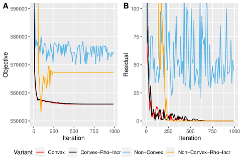
Figure 2: 1000 ADMM iterations on a convex and a non-convex UC instance with and without increasing $\rho$.

To solve the nonconvergence, we iteratively increase the penalty coefficient $\rho$ to force convergence and feasibility. In Xu et al. [2017], it was shown that this helps to achieve faster convergence of convex problems. Figure 2 shows in red the convergence of the solution when 1UC is convex and the nonconvergence (at least not after 1000 iterations) in blue of the non-convex problem. It also shows the convergence of the non-convex problem in orange when $\rho$ is increased. As $\rho$ grows to $\infty$ the constraint violation is encouraged to go to $0$. We start with a small $\rho$ and then iteratively increase it after $m$ iterations. We found that the slower this process goes the better the heuristic solution becomes. The whole procedure is presented in Algorithm 4.

Algorithm 4 ADMM Increasing $\rho$

1:$\rho\leftarrow$ initial $\rho$

2:while  $\sum_{n\in N,t\in T}RD_{nt}>\epsilon$ $\land$ $k<$Max iterations do

3:     for $i\in\{1,\dots,m\}$ do

4:         Gauss Seidel ADMM Iteration

5:         k $\leftarrow$ k + 1

6:     end for

7:     $\rho\leftarrow\alpha\rho$

8:end while

Here $m$ is the number of iterations after we increase $\rho$, by multiplying $\rho$ times $\alpha$. Varying $\alpha$ and $m$ gives us a way to increase and decrease the rate of convergence and therefore the total computation time but at the expense of solution quality.

The intuition is as follows, when solving the subproblems the individual generators, RES and storage units are encouraged to produce power at every time step by the Lagrangian multipliers (when positive) and encouraged to minimize the total residual by the quadratic penalty. Our ADMM algorithm could be interpreted as a greedy algorithm that first steers to the (sub)optimal solution by the Lagrangian multipliers and then steers towards feasibility by increasing $\rho$. Theoretically not much is known about converges or the quality of the solution when applying ADMM to non-convex problems Boyd et al. [2011]. In the next section we will show experimentally that our proposed algorithm gives a fast feasible solution of good quality and scales well with the number of times steps.

5 Computational Experiments

Name	Qudractic Cost	Transmission	Storage	RES	Source
GA10	+	-	-	-	Kazarlis et al. [1996]Rahman et al. [2014]
TAI38	+	-	-	-	Huang et al. [1997]
RCUC50	+	-	-	-	Frangioni et al. [2009]
GMLC73	-	-	-	+	Barrows et al. [2019]
A110	+	-	-	-	Orero and Irving [1997]
KOR140	+	-	-	-	Park et al. [2010]Moradi et al. [2015]
OSTRO187	+	-	-	-	Ostrowski et al. [2012]
RCUC200	+	-	-	-	Frangioni et al. [2009]
HUB223	-	-	-	+	Huber and Silbernagl [2015]
CA426	-	-	-	+	Knueven et al. [2018]
FERC923	-	-	-	+	Knueven et al. [2018]Krall et al. [2012]
RTS26	+	+	-	-	Wang et al. [1995]Wang and Shahidehpour [1993]
RTS54	-	+	-	+	Huber and Silbernagl [2015]
RTS96	-	+	-	-	Pandzic et al.
DSET304	-	+	+	+	Kavvadias et al. [2018]

Table 1: Overview of the instances in the benchmark set. All instances have thermal generators with techno-economic characteristics but only some have a quadratic generation cost, a transmission system, storage or a renewable energy with availability factors. See Wuijts et al. [2021b] for more detail.

To test the efficiency of our proposed algorithms we have performed multiple experiments on 15 well-known benchmark instances found in the literature (Table 1) created by Wuijts et al. [2021b]. We solved the UC instances with our Gauss Seidel ADMM algorithm and with Gurobi with the presented MIL(Q)P formulation (1a) - (1r). Next, we compared the quality of the solutions and the computation times of these algorithms.

First, we experimented with different values of alpha, namely $1.01$, $1.05$, $1.1$ or, $1.2$. Due to the large number of experiments we needed to perform we chose to omit the instances with transmission. Note that as $\alpha$ increases that the computation time and number of iterations decreases. Finally, we performed more detailed experiments for the average value $\alpha=1.1$. For the last experiments we also included the instances with transmission.

All experiments were repeated 10 times to account for the random order of updating the subproblems and the random initial Lagrange multipliers. We set the time horizon to $24,48,\dots,168$ time steps. In all runs, $\rho$ was initially set at $0.0001$ and $m$ at $1$. If $\rho$ was set lower or $m$ higher then the solution quality is better but the algorithm takes more iterations to converge. In preliminary experiments we found that these parameters give a good trade-off between computation time and solution quality except for 1 instance which will be addressed in the next section. Both ADMM algorithms and Gurobi had a time limit of 1 hour.

Gurobi’s MIL(Q)P solver continuously finds heuristic upper bounds and lower bounds until the specified MIP-gap is reached. Our ADMM algorithm produces a single solution, which turned out to be feasible in all our experiments. To compare our ADMM algorithms to Gurobi, we ran the MIL(Q)P model with a MIP-gap of 0 and recorded the intermediate heuristic solutions along with a timestamp at which time they were found. We can then compare the computation times of our ADMM algorithm to the time that Gurobi needs to find a heuristic solution with at most the same value (see Figure 3).

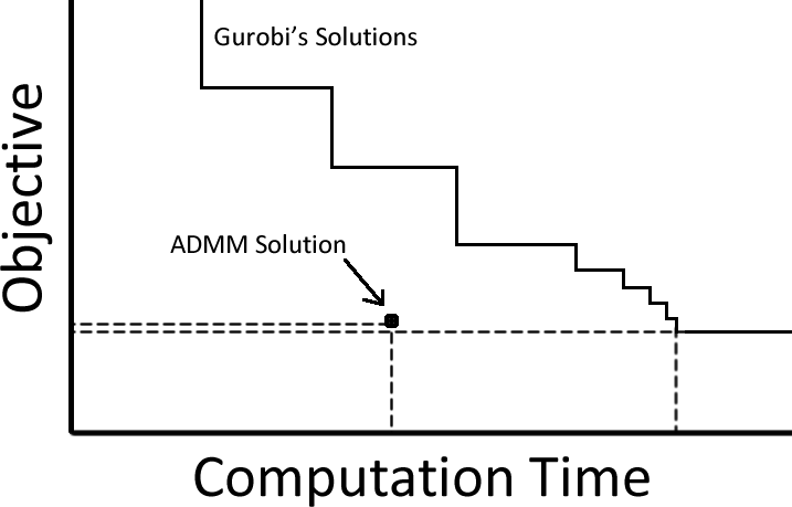
Figure 3: Comparing the ADMM solution to Gurobi.

5.1 Results

Figure 4 and Table 2 show the aggregated results for the instance without transmission and for varying values of $\alpha$. We present the number of iterations, the gap with the optimal (or best known) solution, and the speed-up factor compared to solving the problem by Gurobi.

The figure shows that with increasing $\alpha$ the computation time and number of iterations decreases but the solution quality also gets worse. An $\alpha$ of $1.01$ for example results in small gap indicating high quality solutions but it takes some time for $\rho$ to be of sufficient size that feasibility and convergence is forced. An $\alpha$ of $1.2$ has the opposite effect, the algorithm converges fast, for one instance it was 5801.3 times faster for Gurobi to find a solution of similar quality. However, the average gap is rather large and it has outliers, for example, one solution for UC instance KOR140 was 3.7% removed from the optimal value.

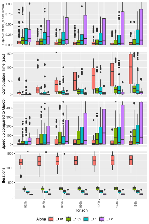
Figure 4: The gap, computation time, speed-up and the number of iterations for varying time horizons and values of $\alpha$ for the 11 instances without transmission.

$\alpha$	Iterations				Gap %				Speedup
	avg	median	min	max	avg	median	min	max	avg	median	min	max
1.01	1229	1239	685	1696	0.07	0.03	0	0.86	29.6	6.0	0.09	271.9
1.05	287	292	154	393	0.09	0.04	0	0.91	108.4	19.4	0.5	1813.1
1.1	163	168	90	216	0.15	0.08	0	1.15	195.3	35.6	0.8	3109.4
1.2	104	100	60	255	0.54	0.13	0	3.7	310.4	43.3	1.0	5801.3

Table 2: Summary of the experiments with varying values of $\alpha$ for the 11 instances without transmission.

Figure 5, Figure 6 and Figure 7 show the results of the experiments where $\alpha$ was 1.1 in more detail. These results also include the four instances with transmission. Detailed results for $\alpha$ set at $1.01$, $1.05$ or $1.2$ would show similar results but with a faster or slower running time and better or worse solution quality according to the trend presented in Table 2.

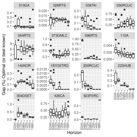
Figure 5: The gap of the objective value of the solution produced by our ADMM algorithm relative to the optimal or best known solution. For these experiments $\alpha$ was set at 1.1.

Figure 5 shows that for most instances the quality is good, for others it is a little worse but still close to optimal while for the instance RTS54 the solutions are far away from the optimum. Even with those outliers on average the algorithm performs well, on average 0.08% away from the optimal value or the best known (Table 2). Moreover, if we choose a different value for $\alpha$ then these gaps would be a lot smaller. In some instances, the solutions produced by our algorithm was the best known. For the instances TAI138, RCUC200, OSTRO178 and KOR140 Gurobi could not find a better solution within the 1 hour time limit for time horizons $>48$.

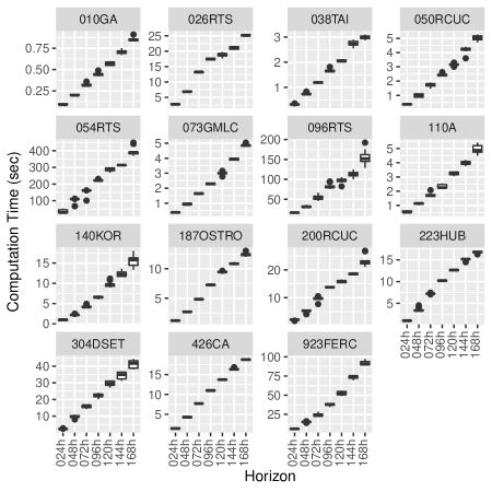
Figure 6: The computation time of all instances with a varying length of the time horizon. For these experiments $\alpha$ was set at 1.1 and for every instance and was repeated 10 times.

Figure 6 presents the computation time increase of our ADMM Gauss Seidel Algorithm when the time horizon increases. For most instances it seems to grow linearly with the number of time steps while for others the growth seems slightly more than linear. Recall from Figure 4 that the number of iterations needed for convergence stays constant when the time horizons increases. However, the computation time of the underlying 1UC subproblem grows when the time horizon increases.

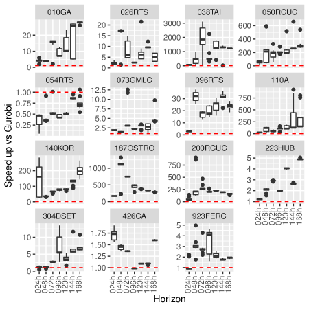
Figure 7: The speedup factor compared to the production of an equal solution by Gurobi. For these experiments $\alpha$ was set at 1.1 and for every instance in was repeated 10 times.

Figure 7 shows how fast our algorithm can find a high quality solution compared to Gurobi. Speedup is defined as the ratio of the computation time of our algorithm and of Gurobi to find a similar solution. The computation time of Gurobi is set at the first time it finds a solution with an objective equal or better than our final objective. For most instances this ratio is large and indicates a large speedup. It seems that our algorithm performs much better than Gurobi on instances with quadratic generation cost. For some instances, especially the ones with linear generation cost, the ratio is smaller and even sometimes below 1. These are for example, RTS54, GMLC73, HUB223, DSET304 CA426, and FERC923. This highlights that for Gurobi solving a MILP is much faster that solving a MIQP. Still even for the instances with linear generation cost the speedup obtained by our algorithm is significant. Moreover, for some cases the speedup increases when the time horizon increases.

Because in the cases Gurobi could not find an equal or better solution within the time limit of 1 hour, we set the computation time to one hour, the real ratios for those instances are larger. Details are presented in Table 3. This also explains the seemingly downward trend of the instances RCUC50, KOR140, OSTRO187 and RCUC200.

Time horizon	24h	48h	72h	96h	120h	148h	168h
GA10	1s	6s	35s	76s	171s	384s	551s
RTS26	59s	0.006%	0.029%	0.069%	0.1%	0.107%	0.111%
TAI38	0.516%	1.356%	1.746%	1.822%	1.922%	2.078%	2.166%
RCUC50	0.031%	0.106%	0.142%	0.177%	0.184%	0.202%	0.25%
RTS54	0.031%	0.084%	0.147%	0.21%	0.236%	0.296%	0.328%
GMLC73	3s	12s	188s	0.044%	0.08%	0.027%	0.078%
RTS96	1.601%	1.766%	1.835%	1.89%	1.921%	2.062%	2.536%
A110	0.001%	0.009%	0.012%	0.014%	0.015%	0.017%	0.02%
KOR140	0.64%	0.929%	1.026%	1.06%	1.109%	1.152%	1.206%
OSTRO187	0.029%	0.05%	0.063%	0.07%	0.115%	0.114%	0.337%
RCUC200	0.091%	0.163%	0.283%	0.308%	11.582%	20.613%	31.123%
HUB223	3s	0.001%	0.001%	0.002%	0.002%	0.001%	0.002%
DSET304	3s	1664s	0%	0%	0.031%	0.03%	0.063%
CA426	6s	62s	118s	197s	406s	615s	971s
FERC923	94s	96s	389s	378s	3601s	1043s	0.001%

Table 3: Computation time for Gurobi to find the optimal solution in seconds. If Gurobi failed to find the optimal solution within 1 hour computation time limit then the MIP-gap is shown.

As our ADMM algorithm with the setting of $\alpha=1.1$ and $m=1$ cannot find a good solution for the instance RTS54, we did additional experiments with $\alpha$ set at 1.05 and m at 5 and presented these much-improved results in Figure 8. However, Gurobi seems just to be very successful at solving this particular instance. But if we consider the speedup, as the time horizon increases, we see that our algorithm gets better relative to Gurobi. This suggests that if we would increase the time horizon even more then it favors our algorithm.

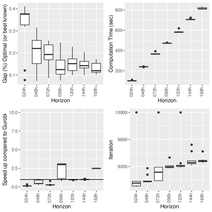
Figure 8: Additional experiments with the UC instance RTS54 with $\alpha=1.05$ and $m=5$

6 Discussion

The results of our new ADMM algorithm for the UC looks promising in comparison with the competing state-of-the-art MIP approach. The advantages of the latter in general are that it can solve large programs, produce near optimal solutions, and can be easily extended. These three advantages also apply to our algorithm; the first two are demonstrated by our results and also our algorithm can easily be extended by implementing new subproblems as a QP or MIQP, as we have shown with the storage units. Additionally, our method has the advantage that solving subproblems can also be improved by using more specific sophisticated algorithms. For example, our 1UC algorithm on average was almost 400 times faster than the MIQP approach Wuijts et al. [2021a].

Moreover, our algorithm seems to scale well with the number of time steps. The previous section showed that the time complexity in practice was almost linear. When solving instances with long time horizons, as is needed in large scale power system modeling, our method can find a high-quality solution in seconds while the MIP solver could not find any good solution even after 1 hour.

For future work this algorithm can be extended or improved in the following way:

• Our algorithm currently does not include reserve requirements. Since reserve requirements are coupling constraints that includes decision variables from multiple components of the power system, we would need to relax these. Moreover, the addition of reserve requirements leads to additional Lagrange multipliers that we need to incorporate into our 1UC dynamic programming algorithm as was previously done by Li et al. [2013].

• Our algorithm currently does not include time dependent start-up cost for the 1UC subproblems but this could be easily incorporated Frangioni and Gentile [2006].

• The subproblems can be modelled in a more complex but also more accurate way. For example, hydropower systems can be modelled in more detail van Ackooij et al. [2018], a more detailed transmission system (DC, AC) can be used, or a more robust transmission system that respect $n-1$ criteria can be modelled Van den Bergh et al. [2014]. Moreover, different power system assets such as demand response can easily be added as a subproblem.

7 Conclusion

In this paper, we presented a new ADMM algorithm that solves UC to near optimality. First, we transformed a standard UC formulation into an augmented Lagrangian formulation by relaxing the demand coupling constraints. Next, we solved the resulting problem with ADMM, an iterative algorithm. In each iteration we solved the subproblems induced by the relaxation of the demand coupling constraints. We used efficient solution methods for them. Especially, the use of our recently introduced fast algorithm for the 1UC subproblem enables many iterations in a limited time, so that ADMM can converge to a feasible solution of high quality. Morover, our algorithms is the first Langrangian beased method that finds feasible solutions for the case where ramping limits are included without requiring an ad-hoc repair heuristic.

Computational experiments on a large set of UC instances showed that our algorithm produces high quality solutions. For instances with linear generation cost it outperformed the state-of-the-art MILP formulation, especially with longer time horizons. For the instances with quadratic cost our algorithms solved those instances significantly faster compared to the state-of-the-art MIQP formulation. As the time complexity of our ADMM grew almost linearly with the number of time steps, it could find high-quality solutions in seconds for instances with long time horizons, while the MIP solver could not find any good solution within one hour.

Our ADMM, therefore, has potential to improve large scale power system modelling commonly based on UC with long time horizons, and planning of unit commitment in the short-term at high temporal resolution. Moreover, due to the decoupled nature of ADMM, the subproblem formulations can easily be adapted, for example to model elements of the power system in more detail or to improve the time complexity of solving the subproblems.

8 Acknowledgement

This work is part of the research programme “Energie: Systeem Integratie en Big Data” with project number 647.003.005, which is financed by the Dutch Research Council (NWO).

Appendix A Variable Splitting and Gauss Seidel

A.1 Multi-block ADMM by Variable Splitting

Another way to decompose a problem with $n$ (sets) of variables is by variable splitting. First, we can rewrite the optimization problem of (2) and (3) (or a problem with $n$ variables) to the following equivalent optimization problem that has additional variables $z_{i}$ that are copies of $p_{i}$:

$$\min\sum_{i=1}^{n}f_{i}(p_{i})$$ (28)

$$s.t.$$

$$D-\sum_{i=1}^{n}z_{i}=0$$ (29)

$$p_{i}=z_{i} \forall i\in\{1,\dots,n\}$$ (30)

Afterwards, we can define the augmented Lagrangian by relaxing (30):

$$\mathcal{L}(\mathbf{p},\mathbf{z},\mathbf{\pi})=\sum_{i=1}^{n}f_{i}(p_{i})+\pi_{i}(p_{i}-z_{i})+\frac{\rho}{2}(p_{i}-z_{i})^{2}$$ (31)

$$\text{s.t. }D-\sum_{i=1}^{n}z_{i}=0$$ (32)

The ADMM iterations are presented in Algorithm 5.

Algorithm 5 Multi-block by Variable Splitting

1:while Stopping criteria have not been met do

2:     for all $i=1,\dots,n$ do

3:         $p_{i}^{k+1}\leftarrow\text{argmin}_{p_{i}}\{f_{i}(p_{i})+\pi_{i}^{k}p_{i}+\frac{\rho}{2}(p_{i}-z_{i}^{k})^{2}\}$

4:     end for

5:     $\boldsymbol{z}^{k+1}\leftarrow\text{argmin}_{z_{1},\dots,z_{n}}\{\sum_{i=1}^{n}\pi_{i}^{k}(p_{i}^{k+1}-z_{i})+\frac{\rho}{2}(p_{i}^{k+1}-z_{i})^{2}\mid D=\sum_{i=1}^{n}z_{i}\}$

6:     for all $i=1,\dots,n$ do

7:         $\pi_{i}^{k+1}\leftarrow\pi_{i}^{k}+\rho(p_{i}^{k+1}-z_{i}^{k+1})$

8:     end for

9:     $k\leftarrow k+1$

10:end while

The optimal values for any $p_{i}$ does not depend on the other production variables because only the copied variables are coupled in (29). Therefore, at each iteration a similar subproblem is solved as when we used the Gauss-Seidel method. However, the difference is that the optimal value for all the copied variables must be found and more Lagrange multipliers must be updated. A main advantage of this method is that:

• At its core it is still 2-block which has convergence guaranties.

• The updates on $p_{1}$, $p_{2}$ ect. can be done in parallel instead of sequential because only the values from iteration $k$ and not from $k+1$ are used.

There seems to be a disadvantage of introducing multiple additional variables and Lagrange multipliers and finding the optimal values of the copied variables at line $5$ in Algorithm 5. However, it is possible to achieve the same effect with only one copied variable and one Lagrange multiplier for each relaxed constraint.

We can rewrite the $z_{i}$ minimization step as follows:

$$\sum_{i=1}^{n}\pi_{i}^{k}(p_{i}^{k+1}-z_{i})+\frac{\rho}{2}(p_{i}^{k+1}-z_{i})^{2}=$$ (33)

$$\sum_{i=1}^{n}\frac{\rho}{2}\left[(p_{i}^{k+1}-z_{i})^{2}+2\frac{\pi_{i}^{k}}{\rho}\left(p_{i}^{k+1}-z_{i}\right)+\left(\frac{\pi_{i}^{k}}{\rho}\right)^{2}-\left(\frac{\pi_{i}^{k}}{\rho}\right)^{2}\right]=$$ (34)

$$\sum_{i=1}^{n}\frac{\rho}{2}((p_{i}^{k+1}-z_{i})+\frac{\pi_{i}^{k}}{\rho})^{2}-\frac{(\pi_{i}^{k})^{2}}{2\rho}$$ (35)

For $z_{i}$ to be optimal, we need to minimize subject to $\sum_{i}^{n}z_{i}=D$. We are minimizing a sum of quadratic differences $p_{i}^{k+1}+\frac{\pi_{i}^{k}}{\rho}-z_{i}$. It is easy to show (by e.g the KKT conditions) that the minimum is attained if all the differences are equal, i.e., the difference would be the same for every $i$ and would be equal to the average difference, which implies

$$p_{i}^{k+1}+\frac{\pi_{i}^{k}}{\rho}-z_{i}=\frac{\sum_{j=1}^{n}(p_{j}^{k}+\frac{\pi_{j}^{k}}{\rho}-z_{j})}{n}$$ (36)

Since the total sum $\sum_{i}^{n}z_{i}$ must be equal to $D$ we can get $z_{i}^{k+1}$ by calculating:

$$z_{i}^{k+1}=\frac{D}{n}+p_{i}^{k+1}+\frac{\pi_{i}^{k}}{\rho}-\frac{\sum_{j=1}^{n}({p_{j}^{k+1}+\frac{\pi_{j}^{k}}{\rho}})}{n}$$ (37)

which simplifies to:

$$z_{i}^{k+1}=\frac{D}{n}-\overline{p}^{k+1}+p_{i}^{k+1},$$ (38)

where $\overline{p}^{k+1}=\sum_{i=1}^{n}p_{i}^{k+1}$

If all multipliers $\pi_{i}$ start with the same value at the beginning of the iteration then the update (Algorithm 3 line 7) would be the same for every multiplier due to (36). This implies that all multipliers have the same value and can be replaced by a single multiplier. Moreover, since the optimal value of $z_{i}^{k+1}$ has an analytical form (38), we can simplify Algorithm 3 to Algorithm 4.

Algorithm 6 Optimal Exchange

1:while Stopping criteria have not been met do

2:     for all $i=1,\dots,n$ do

3:         $p_{i}^{k+1}\leftarrow\text{argmin}_{p_{i}}\{f_{i}(p_{i})+\lambda^{k}p_{i}+\frac{\rho}{2}(p_{i}-\frac{D}{n}+\overline{p}^{k}-p_{i}^{k})^{2}\}$

4:     end for

5:     for all $i=1,\dots,n$ do

6:         $\lambda^{k+1}\leftarrow\lambda^{k}+\rho(\overline{p}^{k+1}-\frac{D}{n})$

7:     end for

8:     $k\leftarrow k+1$

9:end while

In fact Algorithm 4 is called the optimal exchange problem which in turn is a special case of the sharing problem Boyd et al. [2011]. Optimal exchange is similar to Gauss-Seidel, they both have a quadratic constant that is based on the residual load. However, they differ with respect to convergence, as optimal exchange is proven to be convergent, but Gauss Seidel not necessarily. Moreover, finding the optimal value of $p_{1},\dots,p_{n}$ can be done in parallel with optimal exchange but not with Gauss Seidel.

A.2 Gauss Seidel Compared to Variable Splitting

An unexpected result is that the Gauss Seidel outperformed the Exchange ADMM variation by a large margin. Gauss Seidel converged faster and found heuristic solutions of better quality. For most instances the solution found by the Exchange algorithm was far from optimal (Figure 9), while Gauss Seidel found high-quality solutions. Therefore, for the remainder of the results and figures we only show the results of our Gauss Seidel variant.

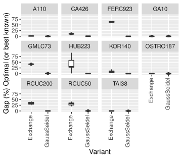
Figure 9: Gap when using the Exchange or Gauss Seidel ADMM variation. Time horizon for experiments were $24$ hours. All instances were repeated 10 times.

References

- van Ackooij et al. [2018] Wim van Ackooij, I Danti Lopez, Antonio Frangioni, Fabrizio Lacalandra, and Milad Tahanan. Large-scale unit commitment under uncertainty: an updated literature survey. Annals of Operations Research, pages 1–75, 2018.
- Melhorn et al. [2016] Alexander C Melhorn, Mingsong Li, Paula Carroll, and Damian Flynn. Validating unit commitment models: A case for benchmark test systems. In Power and Energy Society General Meeting (PESGM), 2016, pages 1–5. IEEE, 2016.
- Welsch et al. [2014] Manuel Welsch, Paul Deane, Mark Howells, Brian Ó Gallachóir, Fionn Rogan, Morgan Bazilian, and Hans-Holger Rogner. Incorporating flexibility requirements into long-term energy system models–a case study on high levels of renewable electricity penetration in ireland. Applied Energy, 135:600–615, 2014.
- Abujarad et al. [2017] Saleh Y Abujarad, Mohammad Wazir Mustafa, and Jasrul Jamani Jamian. Recent approaches of unit commitment in the presence of intermittent renewable energy resources: A review. Renewable and Sustainable Energy Reviews, 70:215–223, 2017.
- Saravanan et al. [2013] B Saravanan, Siddharth Das, Surbhi Sikri, and DP Kothari. A solution to the unit commitment problem—a review. Frontiers in Energy, 7(2):223–236, 2013.
- Padhy [2004] Narayana Prasad Padhy. Unit commitment-a bibliographical survey. IEEE Transactions on power systems, 19(2):1196–1205, 2004.
- Borghetti et al. [2003] Alberto Borghetti, Antonio Frangioni, Fabrizio Lacalandra, and Carlo Alberto Nucci. Lagrangian heuristics based on disaggregated bundle methods for hydrothermal unit commitment. IEEE Transactions on Power Systems, 18(1):313–323, 2003.
- Knueven et al. [2020] Bernard Knueven, James Ostrowski, and Jean-Paul Watson. A novel matching formulation for startup costs in unit commitment. Mathematical Programming Computation, pages 1–24, 2020.
- Atakan et al. [2017] Semih Atakan, Guglielmo Lulli, and Suvrajeet Sen. A state transition mip formulation for the unit commitment problem. IEEE Transactions on Power Systems, 33(1):736–748, 2017.
- Taktak and D’Ambrosio [2017] Raouia Taktak and Claudia D’Ambrosio. An overview on mathematical programming approaches for the deterministic unit commitment problem in hydro valleys. Energy Systems, 8(1):57–79, 2017.
- Morales-España et al. [2013] Germán Morales-España, Jesus M Latorre, and Andres Ramos. Tight and compact milp formulation of start-up and shut-down ramping in unit commitment. IEEE Transactions on Power Systems, 28(2):1288–1296, 2013.
- O’Neill et al. [2011] Richard P O’Neill, Thomas Dautel, and Eric Krall. Recent iso software enhancements and future software and modeling plans. Federal Energy Regulatory Commission, Tech. Rep, 2011.
- Carlson et al. [2012] Brian Carlson, Yonghong Chen, Mingguo Hong, Roy Jones, Kevin Larson, Xingwang Ma, Peter Nieuwesteeg, Haili Song, Kimberly Sperry, Matthew Tackett, et al. Miso unlocks billions in savings through the application of operations research for energy and ancillary services markets. Interfaces, 42(1):58–73, 2012.
- O’Neill [2007] RP O’Neill. It’s getting better all the time (with mixed integer programming). HEPG Forty-Ninth Plenary Session, 16:49, 2007.
- Yang et al. [2022] Yu Yang, Xiaohong Guan, Qing-Shan Jia, Liang Yu, Bolun Xu, and Costas J Spanos. A survey of admm variants for distributed optimization: Problems, algorithms and features. arXiv preprint arXiv:2208.03700, 2022.
- Feizollahi et al. [2015] Mohammad Javad Feizollahi, Mitch Costley, Shabbir Ahmed, and Santiago Grijalva. Large-scale decentralized unit commitment. International Journal of Electrical Power & Energy Systems, 73:97–106, 2015.
- Kraning et al. [2014] Matt Kraning, Eric Chu, Javad Lavaei, Stephen P Boyd, et al. Dynamic network energy management via proximal message passing. Citeseer, 2014.
- Ramanan et al. [2017] Paritosh Ramanan, Murat Yildirim, Edmond Chow, and Nagi Gebraeel. Asynchronous decentralized framework for unit commitment in power systems. Procedia Computer Science, 108:665–674, 2017.
- Zhang and Hedman [2021] Shaobo Zhang and Kory W Hedman. A computational comparison of ptdf-based and phase-angle-based formulations of network constraints in distributed unit commitment. Energy Systems, pages 1–26, 2021.
- Xavier et al. [2020] Alinson S Xavier, Feng Qiu, and Santanu S Dey. Decomposable formulation of transmission constraints for decentralized power systems optimization. arXiv preprint arXiv:2001.07771, 2020.
- Borghetti et al. [2001] A Borghetti, Antonio Frangioni, F Lacalandra, A Lodi, S Martello, CA Nucci, and A Trebbi. Lagrangian relaxation and tabu search approaches for the unit commitment problem. In 2001 IEEE Porto Power Tech Proceedings (Cat. No. 01EX502), volume 3, pages 7–pp. IEEE, 2001.
- Fan et al. [2002a] Wei Fan, Xiaohong Guan, and Qiaozhu Zhai. A new method for unit commitment with ramping constraints. Electric Power Systems Research, 62(3):215–224, 2002a.
- Frangioni et al. [2008] Antonio Frangioni, Claudio Gentile, and Fabrizio Lacalandra. Solving unit commitment problems with general ramp constraints. International Journal of Electrical Power & Energy Systems, 30(5):316–326, 2008.
- Wuijts et al. [2021a] Rogier Hans Wuijts, Marjan van den Akker, and Machteld van den Broek. An improved algorithm for single-unit commitment with ramping limits. Electric Power Systems Research, 190:106720, 2021a.
- Frangioni and Gentile [2006] Antonio Frangioni and Claudio Gentile. Solving nonlinear single-unit commitment problems with ramping constraints. Operations Research, 54(4):767–775, 2006.
- Guan et al. [2003] Xiaohong Guan, Qiaozhu Zhai, and Alex Papalexopoulos. Optimization based methods for unit commitment: Lagrangian relaxation versus general mixed integer programming. In Power Engineering Society General Meeting, 2003, IEEE, volume 2, pages 1095–1100. IEEE, 2003.
- Fan et al. [2002b] Wei Fan, Xiaohong Guan, and Qiaozhu Zhai. A new method for unit commitment with ramping constraints. Electric Power Systems Research, 62(3):215–224, 2002b. ISSN 0378-7796. doi: https://doi.org/10.1016/S0378-7796(02)00043-3. URL https://www.sciencedirect.com/science/article/pii/S0378779602000433.
- Batut and Renaud [1992] J Batut and A Renaud. Daily generation scheduling optimization with transmission constraints: a new class of algorithms. IEEE Transactions on Power Systems, 7(3):982–989, 1992.
- Safdarian et al. [2019] Farnaz Safdarian, Ali Mohammadi, and Amin Kargarian. Temporal decomposition for security-constrained unit commitment. IEEE Transactions on Power Systems, 35(3):1834–1845, 2019.
- Boyd et al. [2011] Stephen Boyd, Neal Parikh, and Eric Chu. Distributed optimization and statistical learning via the alternating direction method of multipliers. Now Publishers Inc, 2011.
- Feltenmark [1997] Stefan Feltenmark. On optimization of power production. 1997.
- Yan et al. [1993] Houzhong Yan, Peter B Luh, Xiaohong Guan, and Peter M Rogan. Scheduling of hydrothermal power systems. IEEE Transactions on power Systems, 8(3):1358–1365, 1993.
- Feltenmark and Kiwiel [2000] Stefan Feltenmark and Krzysztof C Kiwiel. Dual applications of proximal bundle methods, including lagrangian relaxation of nonconvex problems. SIAM Journal on Optimization, 10(3):697–721, 2000.
- Dubost et al. [2005] Louis Dubost, Robert Gonzalez, and Claude Lemaréchal. A primal-proximal heuristic applied to the french unit-commitment problem. Mathematical programming, 104(1):129–151, 2005.
- Liu and Han [2015] Lanchao Liu and Zhu Han. Multi-block admm for big data optimization in smart grid. In 2015 International Conference on Computing, Networking and Communications (ICNC), pages 556–561. IEEE, 2015.
- Chen et al. [2016] Caihua Chen, Bingsheng He, Yinyu Ye, and Xiaoming Yuan. The direct extension of admm for multi-block convex minimization problems is not necessarily convergent. Mathematical Programming, 155(1-2):57–79, 2016.
- Bannister and Kaye [1991] CH Bannister and RJ Kaye. A rapid method for optimization of linear systems with storage. Operations Research, 39(2):220–232, 1991.
- Xu et al. [2017] Yi Xu, Mingrui Liu, Tianbao Yang, and Qihang Lin. No more fixed penalty parameter in admm: Faster convergence with new adaptive penalization. In Advances in Neural Information Processing Systems, pages 1267–1277, 2017.
- Kazarlis et al. [1996] Spyros A Kazarlis, AG Bakirtzis, and Vassilios Petridis. A genetic algorithm solution to the unit commitment problem. IEEE transactions on power systems, 11(1):83–92, 1996.
- Rahman et al. [2014] Dewan Fayzur Rahman, Ana Viana, and Joao Pedro Pedroso. Metaheuristic search based methods for unit commitment. International Journal of Electrical Power & Energy Systems, 59:14–22, 2014.
- Huang et al. [1997] Kun-Yuan Huang, Hong-Tzer Yang, and Ching-Lien Huang. A new thermal unit commitment approach using constraint logic programming. In Power Industry Computer Applications., 1997. 20th International Conference on, pages 176–185. IEEE, 1997.
- Frangioni et al. [2009] Antonio Frangioni, Claudio Gentile, and Fabrizio Lacalandra. Tighter approximated milp formulations for unit commitment problems. IEEE Transactions on Power Systems, 24(1):105–113, 2009.
- Barrows et al. [2019] Clayton Barrows, Aaron Bloom, Ali Ehlen, Jussi Ikaheimo, Jennie Jorgenson, Dheepak Krishnamurthy, Jessica Lau, Brendan McBennett, Matthew O’Connell, Eugene Preston, et al. The ieee reliability test system: A proposed 2019 update. IEEE Transactions on Power Systems, 2019.
- Orero and Irving [1997] SO Orero and MR Irving. Large scale unit commitment using a hybrid genetic algorithm. International Journal of Electrical Power & Energy Systems, 19(1):45–55, 1997.
- Park et al. [2010] Jong-Bae Park, Yun-Won Jeong, Joong-Rin Shin, and Kwang Y Lee. An improved particle swarm optimization for nonconvex economic dispatch problems. IEEE Transactions on Power Systems, 25(1):156–166, 2010.
- Moradi et al. [2015] Saeed Moradi, Sohrab Khanmohammadi, Mehrdad Tarafdar Hagh, and Behnam Mohammadi-ivatloo. A semi-analytical non-iterative primary approach based on priority list to solve unit commitment problem. Energy, 88:244–259, 2015.
- Ostrowski et al. [2012] James Ostrowski, Miguel F Anjos, and Anthony Vannelli. Tight mixed integer linear programming formulations for the unit commitment problem. IEEE Transactions on Power Systems, 27(1):39–46, 2012.
- Huber and Silbernagl [2015] Matthias Huber and Matthias Silbernagl. Modeling start-up times in unit commitment by limiting temperature increase and heating. In European Energy Market (EEM), 2015 12th International Conference on the, pages 1–5. IEEE, 2015.
- Knueven et al. [2018] Bernard Knueven, James Ostrowski, and Jean Paul Watson. On mixed integer programming formulations for the unit commitment problem. E-print, Department of Industrial and Systems Engineering University of Tennessee, Knoxville, TN, 37996, 2018.
- Krall et al. [2012] Eric Krall, Michael Higgins, and Richard P O’Neill. Rto unit commitment test system. Federal Energy Regulatory Commission, 98, 2012.
- Wang et al. [1995] SJ Wang, SM Shahidehpour, Daniel S Kirschen, S Mokhtari, and GD Irisarri. Short-term generation scheduling with transmission and environmental constraints using an augmented lagrangian relaxation. IEEE Transactions on Power Systems, 10(3):1294–1301, 1995.
- Wang and Shahidehpour [1993] Chunyan Wang and SM Shahidehpour. Effects of ramp-rate limits on unit commitment and economic dispatch. IEEE Transactions on Power Systems, 8(3):1341–1350, 1993.
- [53] Hrvoje Pandzic, Yuri Dvorkin, Ting Qiu, Yishen Wang, and Daniel S Kirschen. Unit commitment under uncertainty–gams models. library of the renewable energy analysis lab (real), university of washington, seattle, usa.
- Kavvadias et al. [2018] Konstantinos Kavvadias, Ignacio Hidalgo Gonzalez, Andreas Zucker, and Sylvain Quoilin. Integrated modelling of future eu power and heat systems-the dispa-set v2. 2 open-source model. Technical report, European Commission, 2018.
- Wuijts et al. [2021b] Rogier Hans Wuijts, Marjan van den Akker, and Machteld van den Broek. Effect of modelling choices in the unit commitment problem. Energy Systems, 190:106720, 2021b.
- Li et al. [2013] Zhigang Li, Wenchuan Wu, Boming Zhang, Bin Wang, and Hongbin Sun. Dynamic economic dispatch with spinning reserve constraints considering wind power integration. In 2013 IEEE Power & Energy Society General Meeting, pages 1–5. IEEE, 2013.
- Van den Bergh et al. [2014] Kenneth Van den Bergh, Erik Delarue, and William D’haeseleer. Dc power flow in unit commitment models. TMF Working Paper-Energy and Environment, Tech. Rep., 2014.