A catalogue of observed geo-effective CME/ICME characteristics

Abstract

One of the goals of Space Weather studies is to achieve a better understanding of impulsive phenomena, such as Coronal Mass Ejections (CMEs), in order to improve our ability to forecast them and mitigate the risk to our technologically driven society. The essential part of achieving this goal is to assess the performance of forecasting models. To this end, the quality and availability of suitable data are of paramount importance. In this work, we have merged already publicly available data of CMEs from both in-situ and remote instrumentation in order to build a database of CME properties. To evaluate the accuracy of such a database and confirm the relationship between in-situ and remote observations, we have employed the drag-based model (DBM) due to its simplicity and inexpensive cost of computational resources. In this study, we have also explored the parameter space for the drag parameter and solar wind speed using a Monte Carlo approach to evaluate how well the DBM determines the propagation of CMEs for the events in the dataset. The dataset of geoeffective CMEs constructed as a result of this work provides validation of the initial hypothesis about DBM, and solar wind speed and also yields further insight into CME features like arrival time, arrival speed, lift-off time, etc. Furthermore, the dataset also provides statistical metrics for the DBM model parameters. Also, the probability distribution function for the free parameters of DBM has been derived through a Monte Carlo-like inversion procedure. Probability functions obtained from this work are comparable to distributions employed in previous works. Using a data-driven approach, this procedure allows us to present a homogeneous, reliable, and robust dataset for the investigation of CME propagation. On the other hand, possible CME events are identified where DBM approximation is not valid due to model limitations and higher uncertainties in the input parameters, those events require more thorough investigation.

1 Introduction

ICMEs (Interplanetary Coronal Mass Ejections) are eruptions of plasma and magnetic fields from the Sun’s corona that propagate in the Heliosphere (Webb and Howard, 2012). These plasma and magnetic field structures ejected from the Sun travel through the interplanetary space environment and reach the 1 AU range within 1-5 days (Chen, 2011). In in-situ data, ICMEs can be discerned from the average solar wind by their distinct signatures, such as the enhanced magnetic field, the higher particle speed, and the variations in plasma density (Liu et al., 2010; Papaioannou et al., 2016). They can also be observed remotely by using instruments such as coronagraphs (particularly SOHO/LASCO with coronagraphs C1/C2/C3 Domingo et al. (1995); Brueckner et al. (1995), STEREO/SECCHI with COR1/COR2 Kaiser et al. (2008); Howard et al. (2008) ), and Heliographic imagers (HI1/HI2) (Eyles et al., 2009).

ICMEs are among the main drivers of Space Weather, impacting the space environment and human technology (Gosling et al., 1991; Tsurutani et al., 1988; Schwenn, 2006; Pulkkinen, 2007; Temmer, 2021). The plasma and magnetic fields ejected from the Sun can interact with Earth’s magnetic field, leading to geospace disturbances (Koskinen and Huttunen, 2007), which affect a wide range of technological systems in space, such as satellites, telecommunications, and the GNSS systems (Shea and Smart, 1998; Schrijver and Siscoe, 2010; Aquino and Sreeja, 2013; Piersanti et al., 2017). The present strategies to mitigate the effects of ICMEs on space-based technologies and infrastructures require the knowledge of the ICME arrival time with low uncertainty to allow operators to take action to protect their equipment, by shutting them down or putting them in a safe mode (Barbieri and Mahmot, 2004; Sreeja, 2016; Veettil et al., 2019).

In the last decades, space agencies have designed and launched missions to observe the Sun and monitor the solar wind characteristics, and track CMEs and ICMEs as they travel through space, with the aim to study their interactions with the interplanetary environment. Despite these advancements in space weather forecasting, accurately predicting the characteristics of ICMEs such as their Time-of-Arrival (ToA) and Speed-at-Arrival (SaA) at Earth, as well as the magnitude and direction of the southward component of their magnetic field (which is crucial for determining the intensity of geomagnetic storms Koskinen and Huttunen, 2006), remains a challenging task for the scientific community (Manchester et al., 2017; Riley et al., 2018; Vourlidas et al., 2019).

Following the evolution of numerical methods and the increase of available computational power, a number of empirical methods, physics-based analytical models, and MHD numerical simulations for the ICME kinematics have been developed. In the MHD approximation, the boundary conditions are derived from observed magnetograms and coronographic images and model the propagation of the ejecta by numerically solving the magneto-hydrodynamic equations (ENLIL, HAFv.2 (Hakamada-Akasofu-Fry version 2)+3DMHD, EUHFORIA (EUropean Heliospheric FORecasting Information Asset) Odstrcil et al., 2003; Wu et al., 2007; Pomoell and Poedts, 2018). These simulations allow for the inclusion and consideration of the physical processes being modelled. However, their use requires substantial computing resources due to their computationally intensive nature, making them expensive to run. The complete understanding of the physical processes involved in the Sun-Earth relation relies heavily on numerical modelling techniques. However, with present observation capabilities, the forecasting performance of empirical and analytical methods are comparable to, or in some cases slightly better than, those achieved with numerical methods due to uncertainties in the input parameters (Manchester et al., 2017). This implies that the existing empirical and analytical approaches are still effective and competitive in terms of their predictive capabilities and that the near future of space weather forecasting lies with the use of these computationally light approaches and Machine Learning (ML).

In general, analytical methods are computationally lighter and their parameters can be easily updated with new incoming data. Also, physics-based analytical models (e.g., Vršnak et al., 2013; Rollett et al., 2016; Paouris and Mavromichalaki, 2017; Napoletano et al., 2018) can shed light on the ICME dynamics, and this knowledge would possibly help us in refining also numerical methods. On the other hand, the relationships between ToA and SaA and various CME parameters measured at (or close to) their launch, have been used in empirical prediction methods (e.g., Manoharan, 2006; Gopalswamy, 2009), and most recently in a plethora of ML approaches. ML techniques have become more and more used in space weather, as recently reviewed in Camporeale (2019). In the last years, there have been many attempts to leverage on ML algorithms to obtain the characteristics of an ICME at L1 from the associated CME observables (Bobra and Ilonidis, 2016; Liu et al., 2018; Wang et al., 2019, just to list a few). These ML algorithms use catalogues of CME/ICME characteristics for the training, in order to set their parameters, validate their results and check their performances. Consequently, it becomes more and more important to build CME/ICME databases with a large number of events and small uncertainties (ML methods typically need numerous, relevant and reliable examples in the datasets in order to give accurate results VanderPlas et al., 2012; Ivezić et al., 2014).

In this paper, we present a method to update the catalogue of CME-ICME pairs published in Napoletano et al. (2022), by using a constrained Monte-Carlo strategy to validate its entries. The constrained Monte Carlo strategy allowed us to explore the parameter space in a more effective way. We then make use of this updated catalogue to revisit the Probability Distribution Functions (PDFs) to use for the P-DBM method (Napoletano et al., 2018; Del Moro et al., 2019). Finally, we present a comparison of these PDFs for different solar wind conditions and against previous literature.
The paper is organized as follows. Section 2 describes the DBM model and the mathematical methodology to retrieve PDFs from the catalogue. In Section 3, we analyse the results of the inversion and use them to relabel the CME/ICME catalogue entries and to obtain PDFs for different ICME types. Section 4 is dedicated to conclusions and discussions.
The CME-ICME dataset compiled and used in this work can be found at https://zenodo.org/record/8063404 and a description of the different column headers is provided in the appendix A.

2 Methods

2.1 Drag-Based Model (DBM)

The Drag-Based Model is one of the simplest models that describes CME propagation through the heliosphere. Due to its simplicity and calculation speed, it is one of the most popular models used in CME forecast tools. In recent years, DBM has been used in many studies to describe CME propagation which are summarised in Dumbović et al. (2021).
DBM is based on the assumption that the responsible Lorentz force for CME launch is negligible in the upper part of the solar corona (after a certain heliocentric distance of 20 R$\odot$, but this assumption is not always valid as for many events Lorentz force is still comparable with drag force and upper limit of the heliocentric distance vary from event to event Vršnak (2001); Vršnak et al. (2004); Sachdeva et al. (2015, 2017) ) and beyond this heliocentric distance the dynamics of the ICME is dominantly governed by its interaction with ambient solar wind via MHD drag (Cargill, 2004; Vršnak et al., 2013). Due to MHD drag force ICMEs that are faster (slower) than solar wind have a tendency to decelerate (accelerate) during propagation, which was also supported by observations (Gopalswamy et al., 2000). CME radial acceleration according to the DBM approach is given as:

$$a(r)=-\gamma\bigg{(}v(r)_{CME}-w\bigg{)}\mid v(r)_{CME}-w\mid$$ (1)

where $a(r)$ and $v(r)_{CME}$ are the instantaneous acceleration and speed of ICME, respectively, $w$ is the instantaneous ambient solar wind speed, $\gamma$ is the drag parameter that is also called as drag efficiency. It is important to note that all the quantities in equation 1 are space and time-dependent. Also, beyond 20 R$\odot$, $\gamma$ and $w$ may be approximated to be constant throughout the heliosphere (Cargill, 2004; Vršnak et al., 2013). Under such approximation, equation 1 can be solved analytically to obtain heliospheric distance and speed of ICME as a function of time (Vršnak et al., 2013):

$$v(t)=\frac{v_{0}-w}{1\pm\gamma(v_{0}-w)t}+w$$ (2)

$$r(t)=\pm\frac{1}{\gamma}\ln(1\pm\gamma(v_{0}-w)t)+wt+r_{0}$$ (3)

where $\pm$ sign accounts for accelerated/decelerated CMEs i.e., plus for v${}_{0}>$ w and minus for v${}_{0}<$ w. Eqns. 2 and 3 give us the speed and distance as a function of CME propagation time from an initial distance (at t=0) r₀ and take-off speed v₀. From those, one can determine the transit time $t_{1AU}$ and impact speed $v_{1AU}$ at 1AU.

2.2 DBM Inversion Procedure

DBM solution, as given in Vršnak et al. (2013), can be used to obtain the analytical values of free DBM parameters. If the ICME follows the DBM model, and if its boundary conditions, i.e, initial position $r_{0}$, initial speed $v_{0}$, ToA $t_{1AU}$ and impact speed $v_{1AU}$ are known, then the free parameters of the model, namely drag parameter $\gamma$ and solar wind speed $w$, can be obtained via a mathematical inversion of the set of equations presented above (eqs. 2 and 3).

$$\frac{(v_{0}-w)(v_{1AU}-w)t_{1AU}}{(v_{0}-v_{1AU})}\ln\left[\frac{(v_{0}-v_{1AU})}{(v_{1AU}-w)}+1\right]+wt_{1AU}+r_{0}-r_{1AU}=0$$ (4)

The above equation 4 is solved numerically to obtain $w$, then using equation 5 is used to directly compute $\gamma$:

$$\gamma=\frac{(v_{0}-v_{1AU})}{(v_{0}-w)(v_{1AU}-w)t_{1AU}}$$ (5)

2.3 Mathematical Framework

In search for the unique distribution for the free DBM parameters, we applied the DBM inversion procedure to the existing dataset, published in the previous works of Napoletano et al. (2018) and Napoletano et al. (2022). A comprehensive description of a dataset is provided in appendix A, while the summary of a few particular quantities used in this study and associated results are tabulated in table 4. In the process of DBM inversion, we discovered that the majority of the CME events in the dataset lack analytical solutions for the equations 4 and 5. This is unexpected, since ”DBM is (reasonably) valid during CME propagation for all the CME events” is a null hypothesis for the dataset. The reason behind this discrepancy is that errors associated with the initial position ($r_{0}$), target position ($r_{1}$), transit time (t_1AU), impact speed ($v_{1}$) and initial speed ($v_{0}$) were not taken into account in the inversion procedure. Another possible reason is that DBM is not properly describing the CME motion (e.g, $w=$ constant is not a realistic approximation; CME-CME interaction is also possible).

However, for this work, we adhere to our null hypothesis and consider the possibility of including uncertainties for the measured CME features. To incorporate the errors associated with those quantities, we adapted a pairwise selection approach. It is worth noting that Napoletano et al. (2022) also adopted a probabilistic approach in the inversion procedure to obtain $w$ and $\gamma$. In order to do that, they assumed that [$r_{0},r_{1},v_{0},v_{1},t_{1AU}$] follows a normal distribution and draw random samples, here the majority of samples are concentrated in the part of the Gaussian curve peak. However, our pairwise approach allowed us to explore other parts of parameter space where less probable values exist. We have assumed that two parameters, $r_{0}$ and $r_{1}$, do not suffer any errors because their values are fixed. We took $r_{0}$ = 20 R$\odot$ and, for $r_{1}$ we have used the actual Sun-Earth Distance at a time when CME is at $r_{0}$. The arrival speed of CME in the dataset is calculated as a mean of solar wind speed during a disturbance in plasma and therefore it has associated intrinsic error. The error associated with arrival speed is relatively small compared to the initial speed and arrival time, therefore it is neglected in the study. Therefore, we end up with only two quantities, $v_{0}$ and $t_{1AU}$ which have larger errors. Next, we made a pairwise selection of ($t_{1AU},v_{0}$) for each DBM inversion iteration from the normal distribution followed by both quantities where $\mu$ is the observed value (”Transit_Time” and ”v_r” is taken as $\mu$) and $\sigma$ is an error associated with the observed quantity (”Transit_time_err” and ”v_r_err” taken as $\sigma$). It is important to keep in mind that the tails of the normal distribution function are 3$\sigma$ width. For a pairwise selection, we draw 200 samples for t_1AU and the same for $v_{0}$. So in the end, we have a total of 40,000 possible pairs. After this pair selection, we performed the DBM inversion to obtain values of $w$ and $\gamma$, respectively.

The DBM inversion procedure is a Monte Carlo process and after the inversion procedure, we have 40,000 possible solutions for $w$ and $\gamma$. Many of these values can not be physically feasible, for example, negative values of $w$. Vršnak et al. (2013) provided a brief description of their work, and from there we deduced that the drag parameter $\gamma$ has a relation with the mass of the CME. In our primary analysis, we found that the inversion procedure also provides very high values for $\gamma$ which can not be explained by the typical mass range of CMEs. Therefore, it is necessary to employ constraints on the values obtained through the inversion procedure. The constraints that we imposed on inversion values are given below.

1. 0 $\leq$ $w$ $\leq$ $1000$ km/s
   Solar wind speed cannot be negative and the typical speed for fast solar wind in literature is $800km/s$. It is worth noting that the condition of realistic solar wind speed in Paouris et al. (2021) is 300-600 $km/s$ which is very narrow compared to us.

2. $0.1\times 10^{-7}$ $\leq$ $\gamma$ $\leq$ $3.0\times 10^{-7}$ km^-1
   It is important to note that the typical range for the $\gamma$ parameter, in Vršnak et al. (2013), is $0.2-2.0\times 10^{-7}$, but we widen this range to accept a few more extreme solutions. Similarly, Paouris et al. (2021) has a range of $0.01-0.59\times 10^{-7}$ for realistic drag parameter but their obtained values are in the range of $0.21-0.42\times 10^{-7}$ (see table-4 of (Paouris et al., 2021)) which is comparable to our range.

After this, we derive the four main quantities namely $W_{mean}$, $\gamma_{mean}$, $W_{opt}$ and $\gamma_{opt}$ from the accepted values of $w$ and $\gamma$; the $opt$ values correspond to the DBM input that produced the minimum deviation from the observed transit time. In order to evaluate the ”goodness” of the inversion procedure, we define the ”Acceptance Rate” as the ratio between the number of meaningful solutions to the total number of possible solutions, represented by the number of samples.

$$\textrm{Acceptance\, Rate}(AR)=\frac{\textrm{no. of physically feasible solutions}}{\textrm{Total no. of solutions}}=\frac{m}{n\times n}$$ (6)

Here, $m$ is the no. of solutions accepted after applying constrain and $n$ is no. the of samples drawn from the $t_{1AU}$ and $v_{0}$ distributions each. Figure 1 shows the flow diagram for the DBM inversion procedure that we implemented on the CME dataset and how the results of the inversion procedure are analysed.

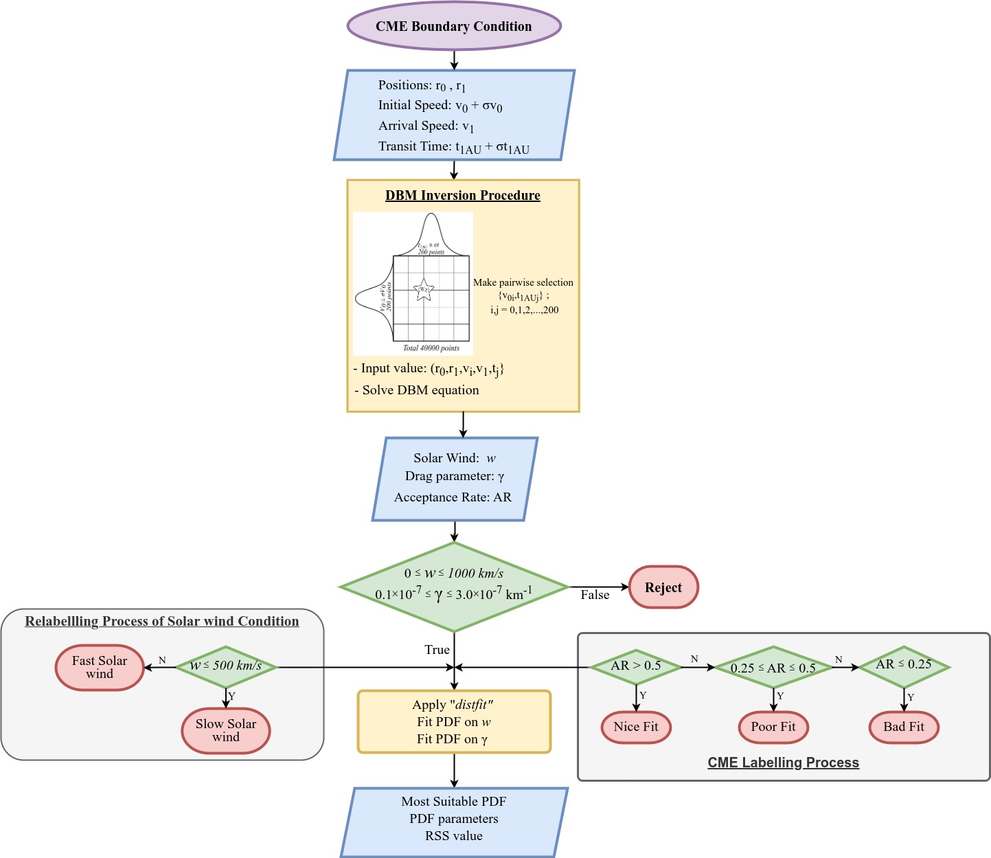
Figure 1: Schematic of DBM inversion procedure. The values of boundary conditions are fed into the equations 4 and 5 using a pairwise approach to obtain $w$ and $\gamma$. The obtained values are checked for selection criteria. The accepted values are used to determine the solar wind condition, the most suitable PDF of model parameters and CME labelling scheme.

3 Results

3.1 Inversion Procedure Results

The inversion procedure was performed on the entire CME-ICME pair catalogue and it turned out to be successful for 204 out of 213 events. At the end of the inversion procedure, we obtained $3,664,748$ possible values of $w$ and $\gamma$ that enable us to provide a statistical distribution for them. In fig 2, the ($\gamma$,$w$) phase space for the entire ICME dataset is shown and there we can identify the trend line for a few individual CMEs. From the DBM equation 1, one can easily notice that CME either accelerate or decelerate during their propagation. Based on these propagation conditions, we derived two different distributions divided into accelerated and decelerated CMEs. Furthermore, a free DBM parameter $w$ can also be divided into two groups called the slow and fast solar wind, and therefore we can draw two more joint distributions based on solar wind speed conditions.

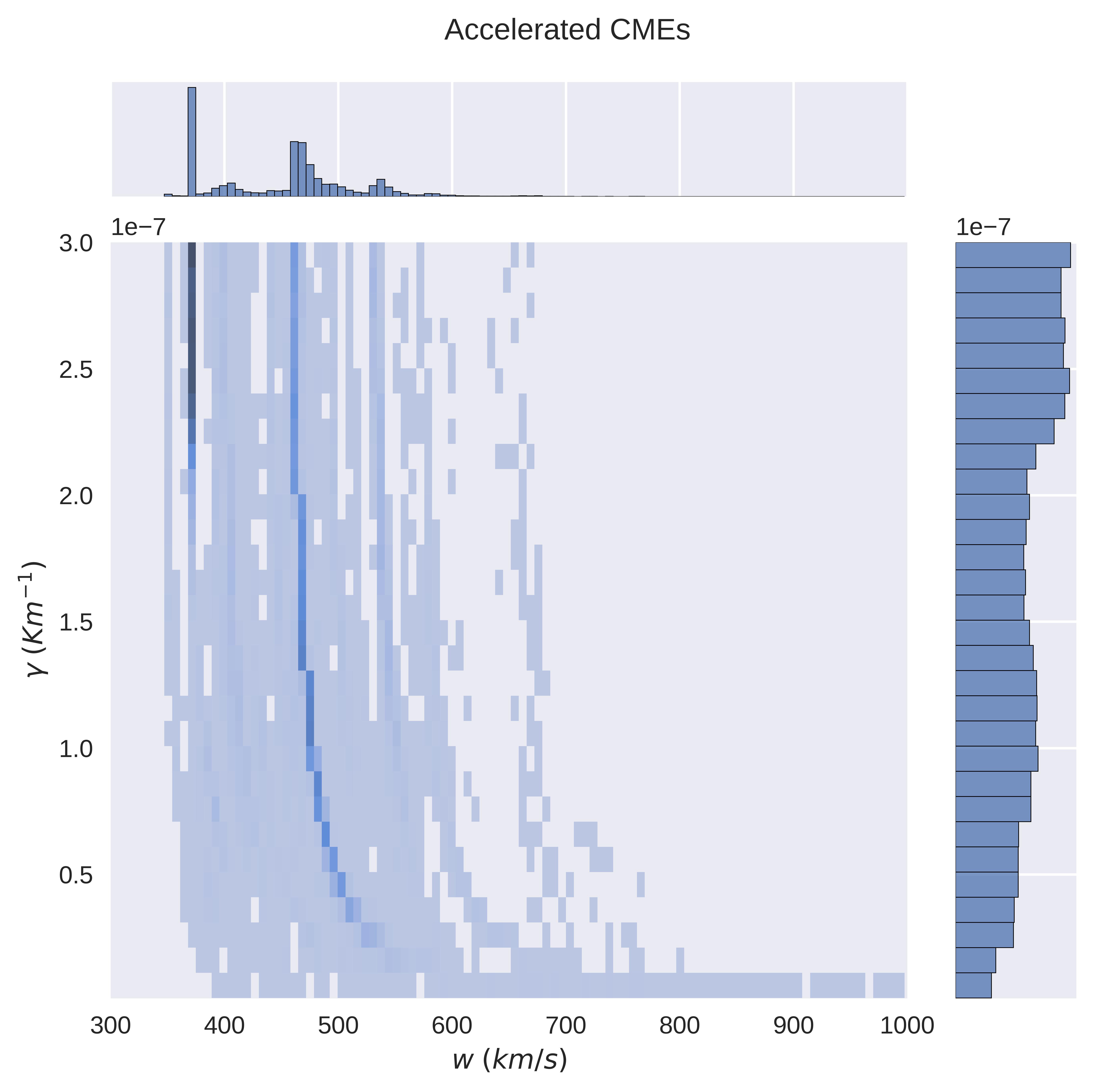
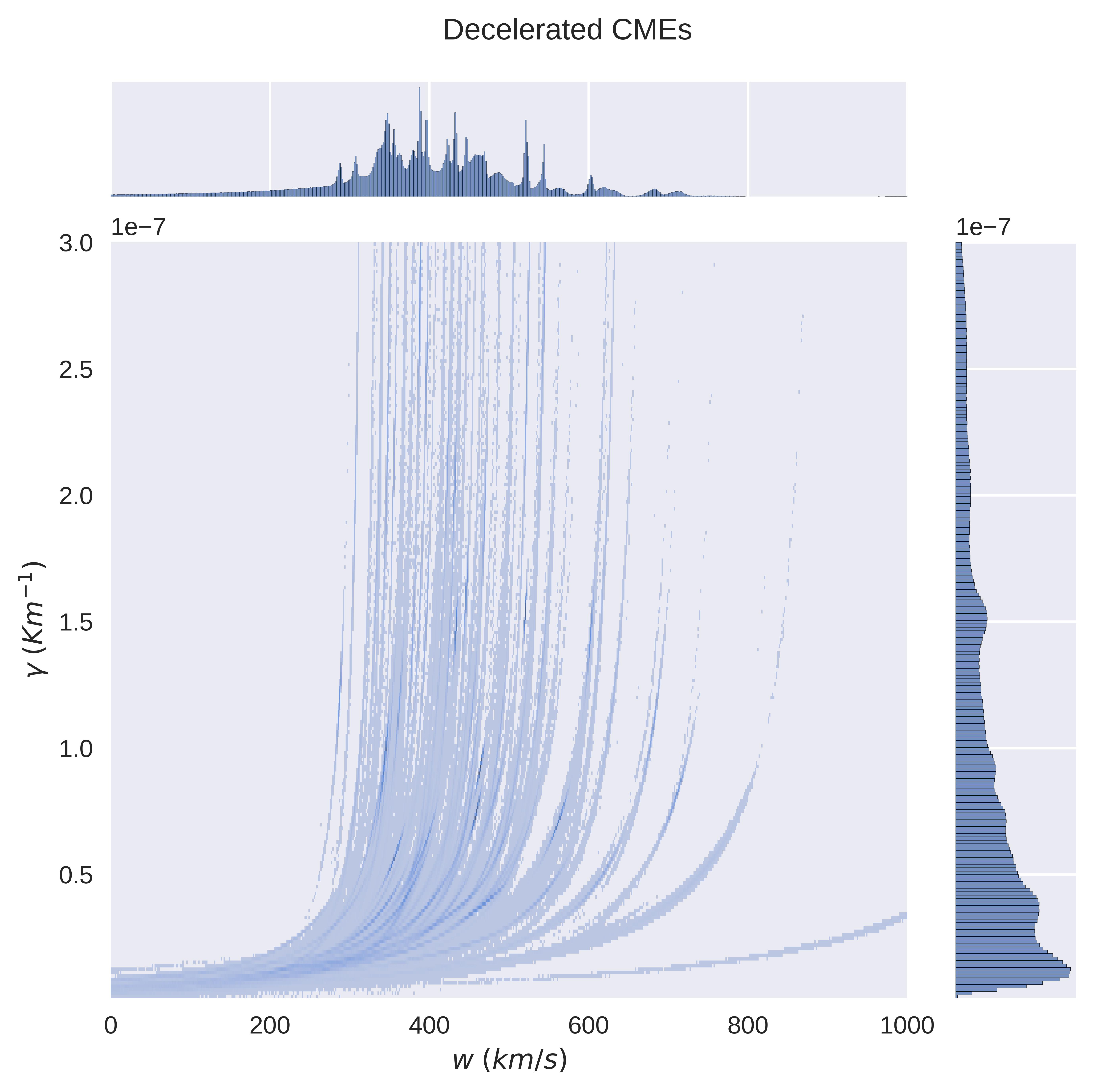
Figure 2: Joint distribution of ($\gamma$,$w$) from the inversion procedure. Left Panel:($\gamma$,$w$) Phase space for whole dataset (3644748 values) Middle Panel:($\gamma$,$w$) phase space for the dataset of accelerated CMEs (25428 values) Right Panel:($\gamma$,$w$) phase space for the dataset of decelerated CMEs (3619320 values)

3.2 Determining the quality of inversion process for each CME event

It is important to note that, we claimed that the DBM inversion was successful for 204 events and therefore there should be $8,160,000$ possible values of $\gamma$ and $w$ that are more than double the numbers we have obtained from the DBM inversion procedure. This discrepancy is due to the fact that there are many pairs for which the DBM inversion procedure is not successful or the obtained values of ($\gamma$,$w$) are discarded as they did not fulfil the constraints. This can also be observed in the ($\gamma$,$w$) phase space of different CME events. Based on the density in the ($\gamma$,$w$) phase space, we label the event as ”Nice Fit”, ”Poor Fit” and ”Bad Fit”. This labelling helps us to determine which CME event in the database follows the DBM hypothesis. To stay consistent in the labelling procedure, we used the Acceptance Rate (AR) defined by the equation 6. The description for the labels is as follows.

1. Nice Fit: AR $>$ 0.5; the DBM approximation is very well valid for this kind of CME event as the inversion procedure is successful for more than 50 $\%$ of the pairs. Therefore, there is a very sharp trendline in ($\gamma$,$w$) phase space.

2. Poor Fit: 0.25 $\leq$ AR $\leq$ 0.5; the DBM is reasonably valid as one can still see the trendline in ($\gamma$,$w$) phase space.

3. Bad Fit: AR $<$ 0.25; the DBM approximation is less applicable for the events and it is hard to find the trend line in phase space.

Figure 3 shows event counts in each assigned label. We want to stress here the fact that, this labeling scheme is a key point for the database that is created as a result of this work. This labeling helps us to determine which CME event in the database follows the DBM. Events that are flagged as ”Poor Fit” or ”Bad Fit” are required further investigation. Hereafter, we only focused on the Nice Fit events to obtain the PDFs for $w$ and $\gamma$ as it helps to improve the PDFs. Eventually, these better statistics will lead to better accuracy in CME arrival forecasting.

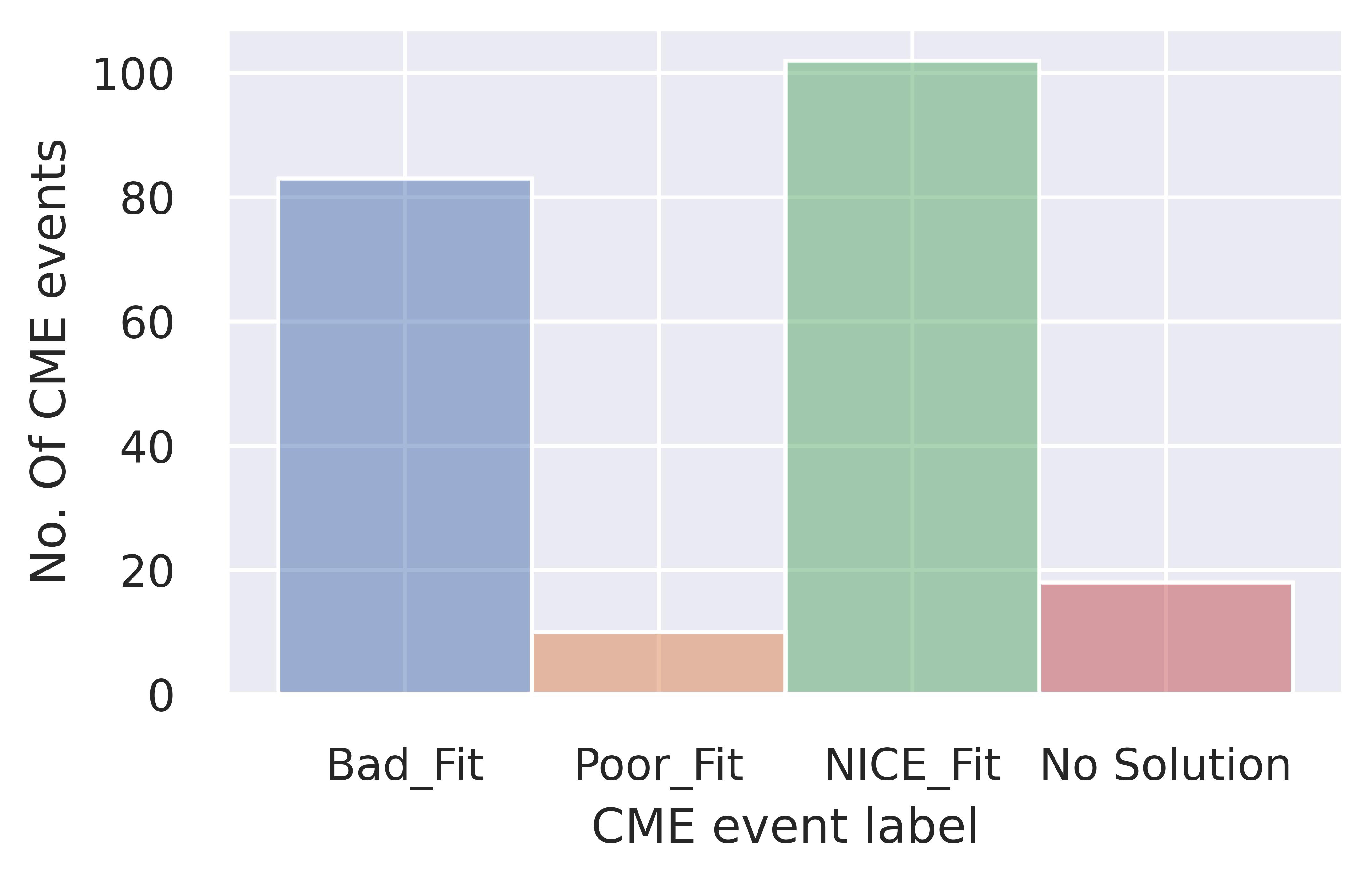
Figure 3: Histogram showing a number of events in the ”Nice Fit”, ”Poor Fit” and ”Bad Fit”.

3.3 Relabelling the Solar Wind condition

We found that there are only 28 CME events that are accelerating during propagation, these are around 13% of the entire dataset, therefore statistics for accelerating CMEs are not very well resolved. In order to find a distribution for the free DBM parameters we established a group of CME based on solar wind conditions. A dataset that is already obtained as a part of previous work of Napoletano et al. (2022) contains information about the solar wind speed type ( See Appendix-A Column: SW_type -S/F) based on the presence of Coronal Holes close to the source of a CME. The group of CMEs formed based on coronal hole presence data provides two completely overlapping distributions for fast and slow solar wind speeds. This contradicts our current physical understanding of solar wind. Furthermore, the large standard deviation makes the model unsuitable for precise and reliable real-time space weather forecasting applications. Therefore we relabel the solar wind type associated with each CME by using threshold $W_{sim}\geq$ 500 km/s to discriminate the fast solar wind from the slow one. This threshold is similar to one that is used in Napoletano et al. (2018). In figure 4 ($\gamma$,w) phase space is shown for the two ”SW_type” and ”Wind_type” solar wind labeling. One important point to note here is, the tail part of any distribution in a negative region is due to the plotting style not due to the presence of any value. Also, from now onward we focus on this new labeling scheme for solar wind speed.

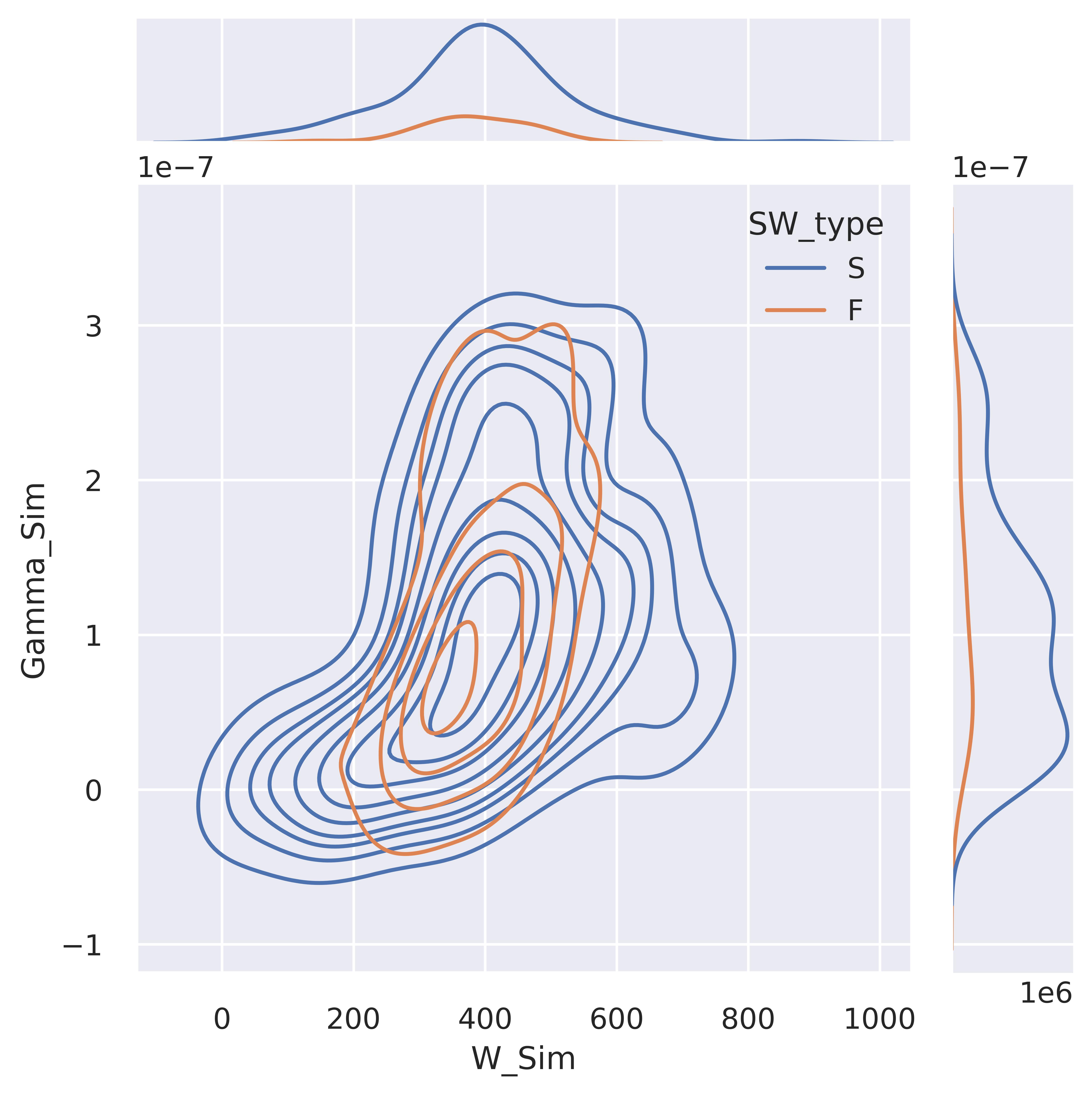
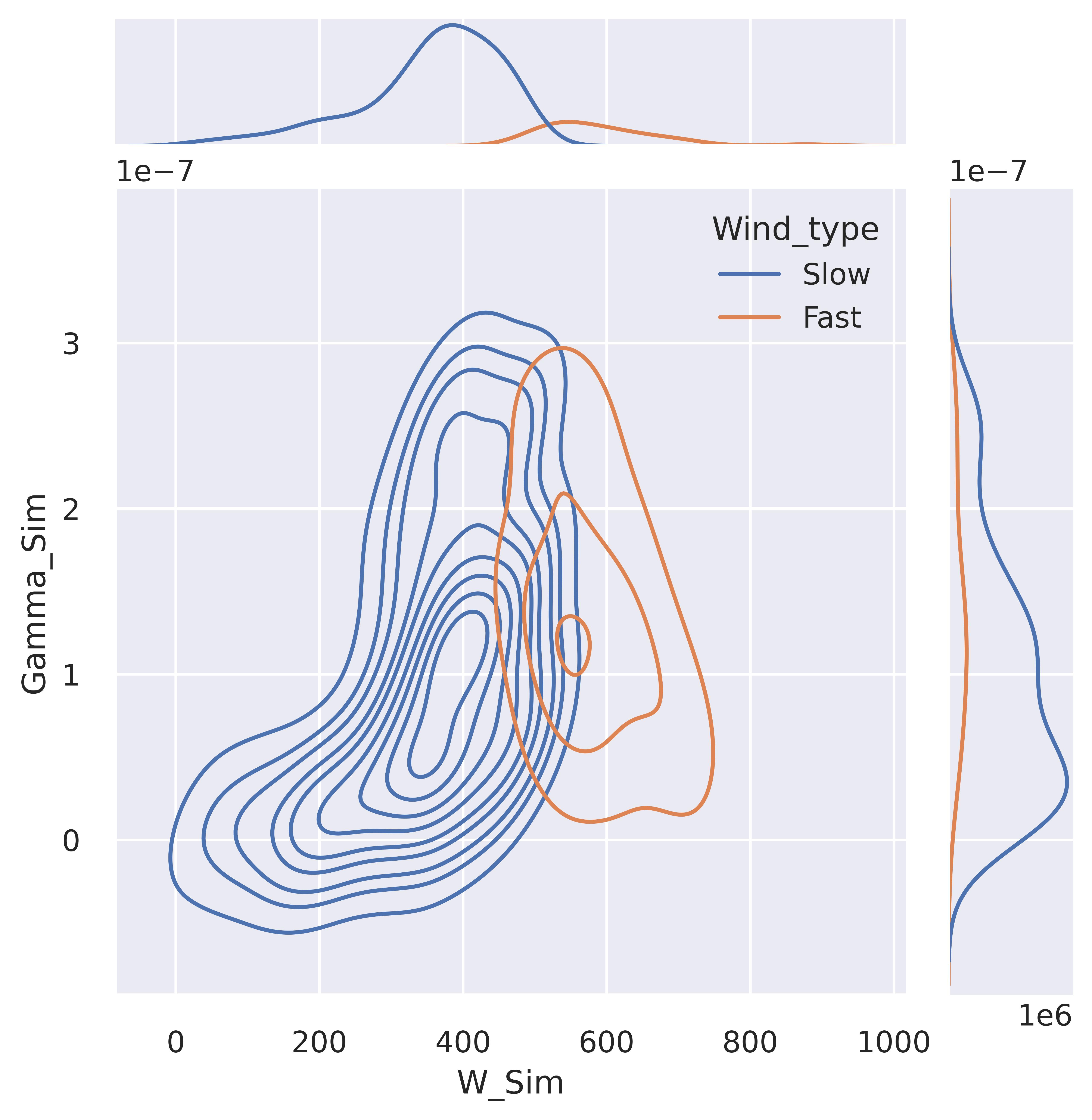
Figure 4: ($\gamma$,$w$) Phase space in different solar wind speed condition labeling scheme. On the x-axis, W_sim shows solar wind speed obtained from a DBM inversion with a unit of km/s while on the y-axis drag (Gamma_sim) value obtained from the inversion procedure is shown on a unit scale of km^-1

3.4 PDF for Solar wind Speed

From the joint distribution shown in figure 2, we can extract a distribution function for the solar wind speed $w$. Here, we have fitted Gaussian, Student-t and Lognormal functions to the distribution function as these three functions returned a better fit among different PDFs available in the distfit package (Taskesen, 2023). In figure 5, the histogram obtained from the dataset and fitted PDFs are shown. Here we have considered the RSS (Residual Sum of Squares) value to determine which one is the best fit. In most cases, all 3 distribution functions show a similar RSS value which is clear from the figure as well. So, in the end, we concluded to select the Gaussian distribution function for the solar wind speed $w$ to be consistent with previous works of, e.g., Napoletano et al. (2018), Dumbović et al. (2018), Dumbović et al. (2021), Napoletano et al. (2022).

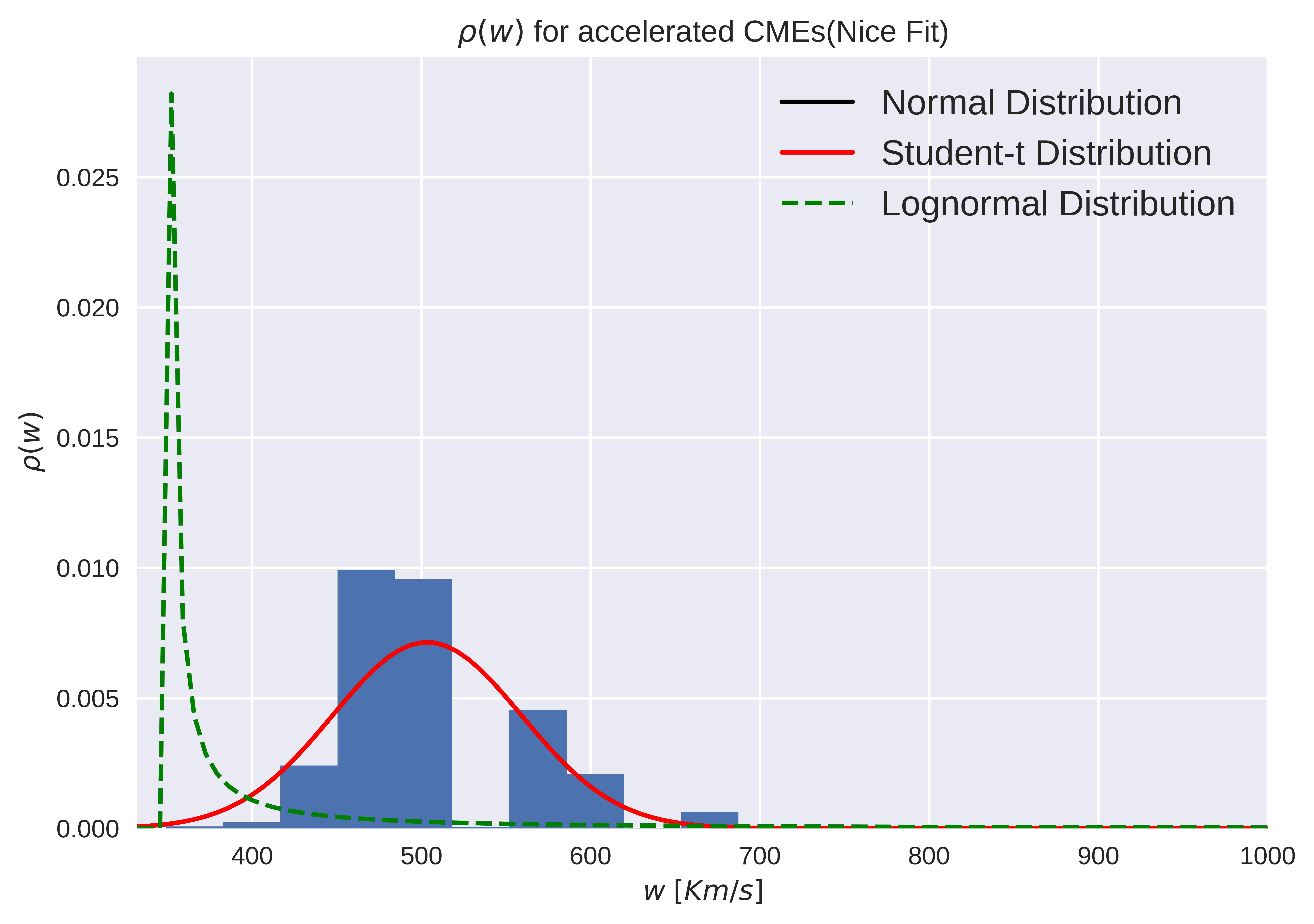
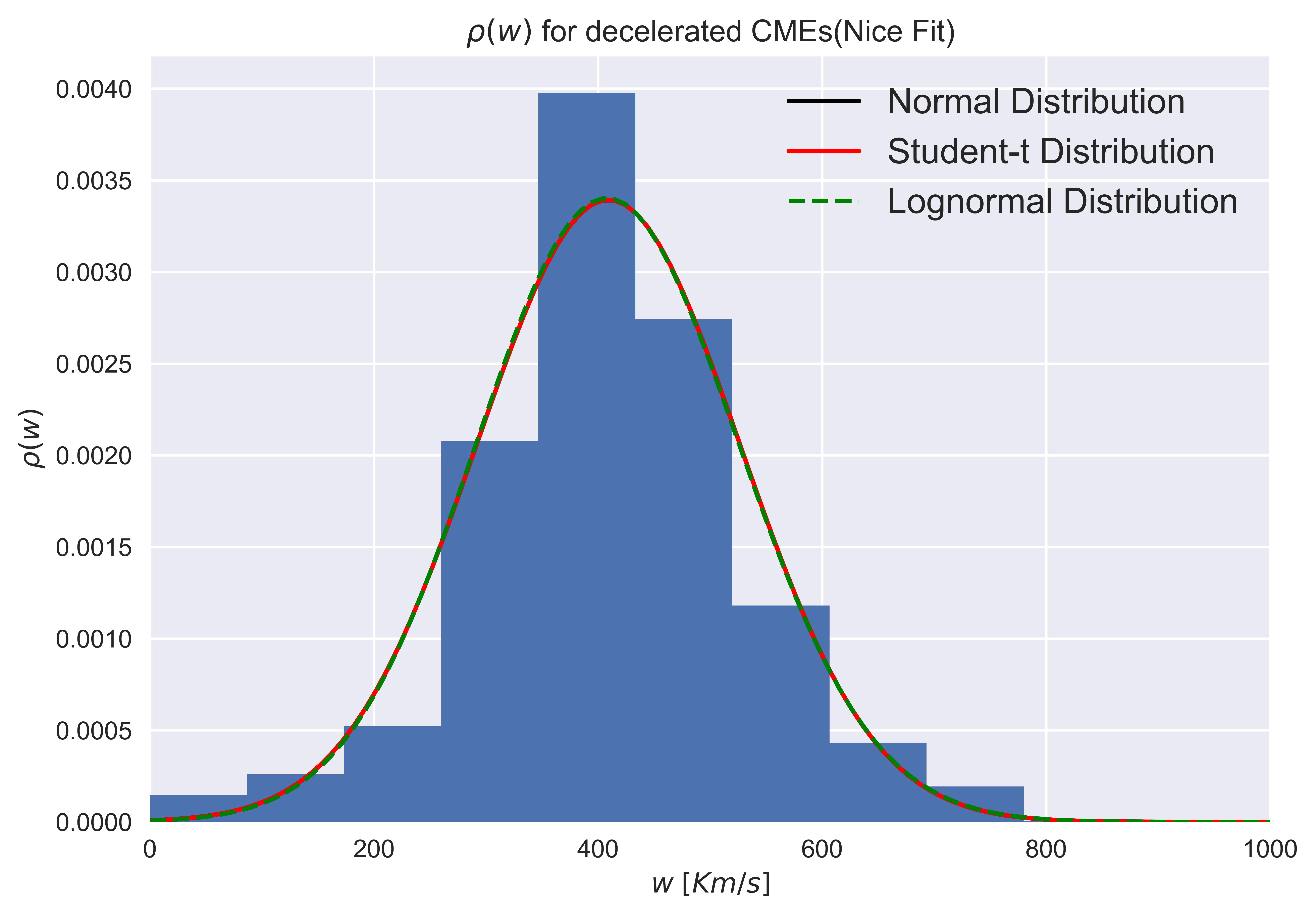
Figure 5: Probability distribution functions for solar wind speed $w$ for accelerated and decelerated CMEs with a kernel density $\rho$ on the Y-axis. Left: $w$ PDFs for accelerated CMEs with Nice Fit label. Note that the normal and student-t distributions overlap with each other Right: $w$ PDFs for decelerated CMEs with Nice Fit label. All three distribution functions overlap with each other. The overlapping of functions is evident through RSS values.

We categorized our dataset into Slow and Fast CMEs based on the ambient solar wind condition experienced by the CME during its propagation (using a threshold of 500km/s to separate fast and slow solar wind conditions), as described before in this section., and attempted again to fit the same three distribution functions. Unlike the prior attempt, the fitting’s RSS value is not the same for slow and fast solar wind conditions. For slow CMEs, the ”student-t” distribution describes the best PDF while for fast CMEs the lognormal function is the most suitable PDF. Here, we only emphasize the fact that ”student-t” and ”lognormal” distributions are the best fits and are strongly biased by the hard thresholding. In figure 6 PDFs for the slow and fast solar wind conditions are shown. The parameters for the fitted distributions are reported in table 1.

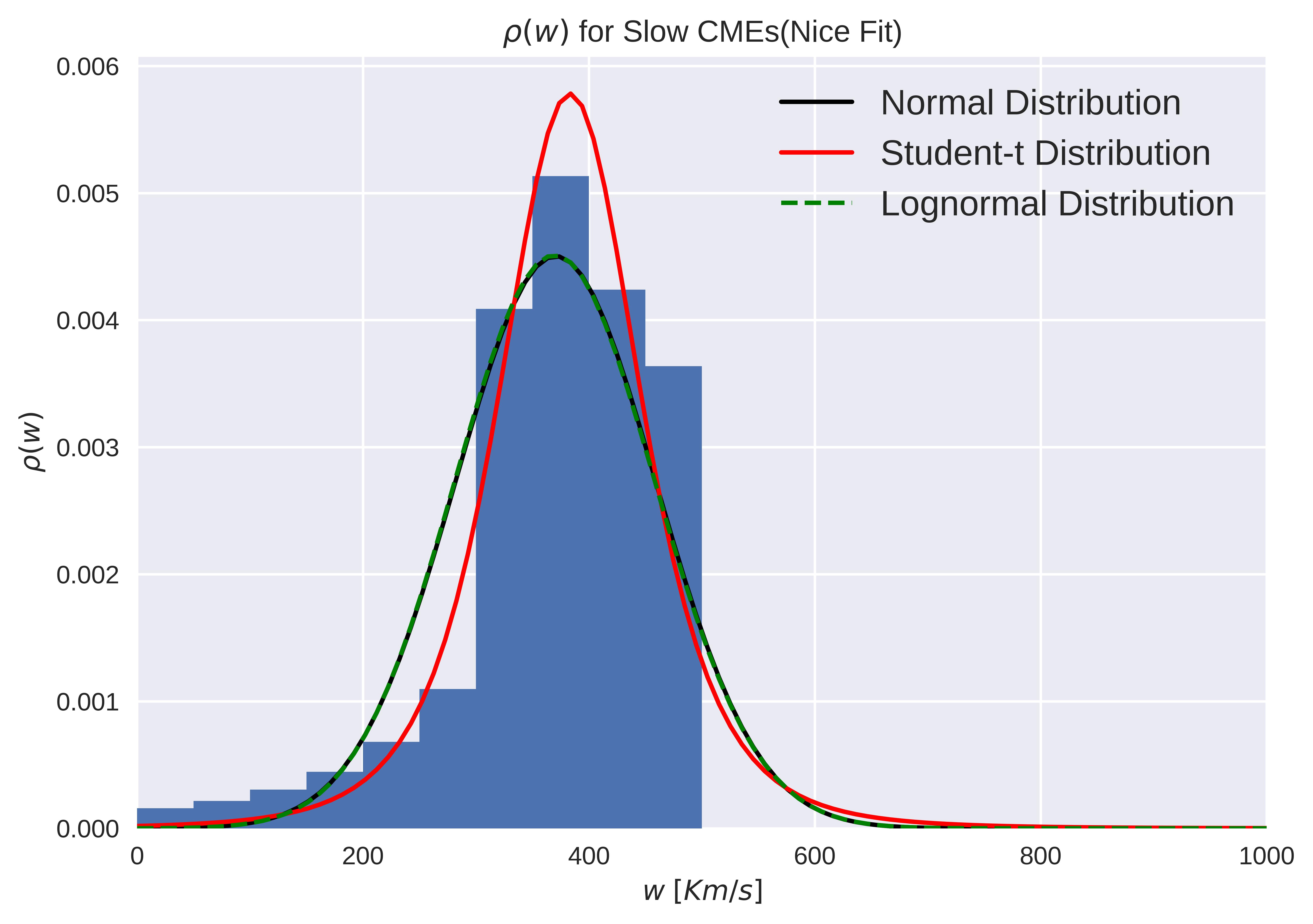
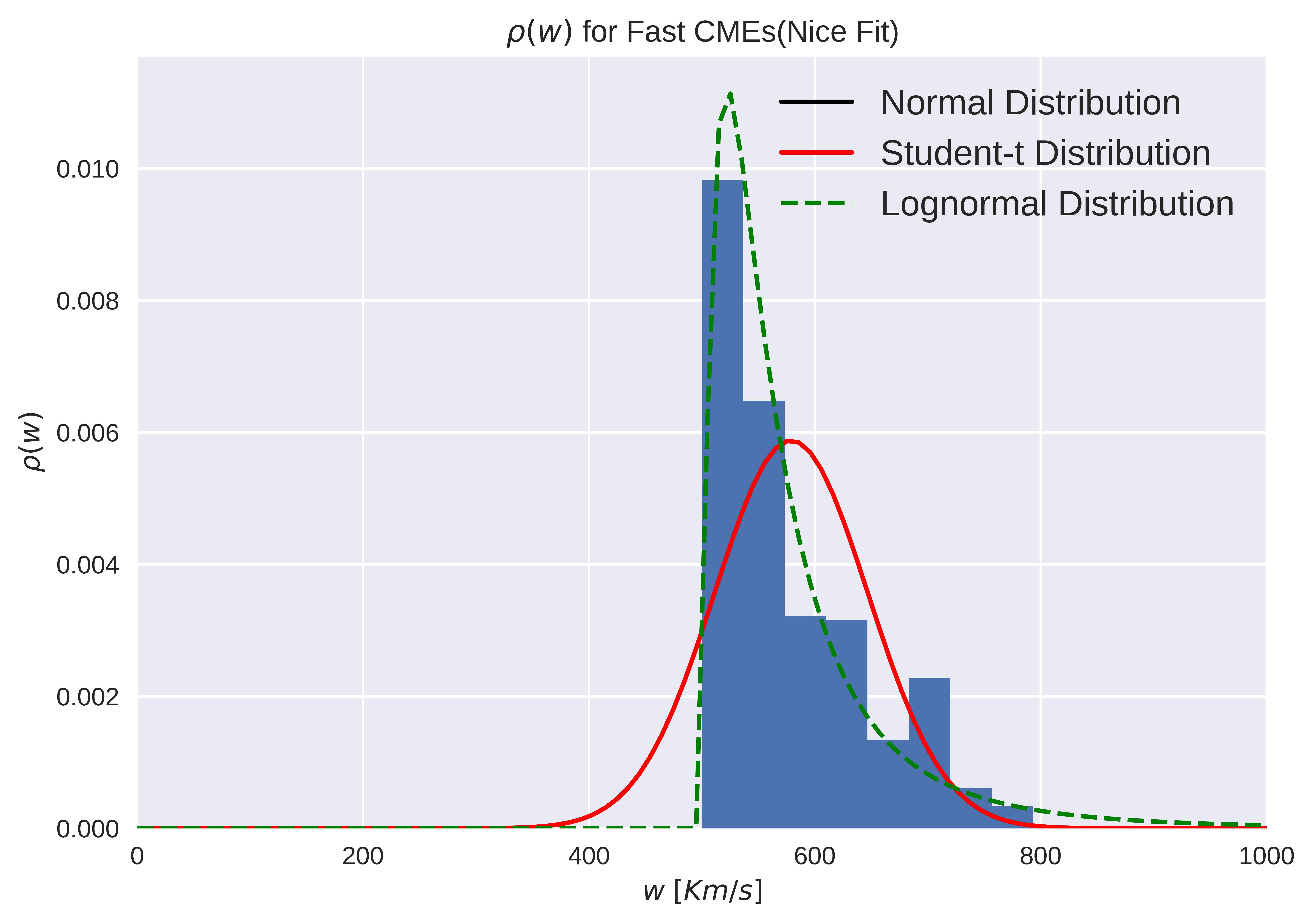
Figure 6: Probability distribution functions for solar wind speed $w$ for slow and fast CMEs. Left: $w$ PDFs for slow CMEs with Nice Fit label. Right: $w$ PDFs for fast CMEs with Nice Fit label. (In both cases the Normal and Student-t functions overlapped with each other)

Table 1: Parameters for the different functions used to model the Solar wind speed distribution. For the Lognormal function, tabulated values can not be used directly as average and standard deviation. The transformation from the fitting parameters to values used in the model can be done by the equation 10.

CME Group	PDF	$\bar{w}[Km/s]$	$\sigma_{w}[Km/s]$	Args	RSS
Accelerated	Normal	503.356	55.848	-	0.000538
	Student’s-t	503.356	55.848	1.526$\times 10^{6}$	0.000538
	Lognormal	-0.407	3.910	349.009	0.001469
Decelerated	Normal	409.168	117.545	-	0.00046
	Student’s-t	409.168	117.543	1.479$\times 10^{5}$	0.00046
	Lognormal	9.524	0.009	-1.328$\times 10^{4}$	0.000458
Slow	Normal	370.530	88.585	-	0.000714
	Student’s-t	383.169	64.944	4.101	0.000622
	Lognormal	9.784	0.005	-1.738$\times 10^{4}$	0.00072
Fast	Normal	579.058	67.871	-	0.002862
	Student’s-t	579.058	67.872	1.837$\times 10^{6}$	0.002862
	Lognormal	4.084	0.883	494.597	0.001934

Paouris et al. (2021) has studied the same 16 CME-ICME events from the Dumbović et al. (2018) to compare the performance of the Effective Acceleration Model (EAM) with Drag Based Ensemble Model (DBEM). They have also performed the inversion technique to find optimal values of solar wind speed $w$ and drag parameter $\gamma$. In the table 2 below optimal values of $w$ from different studies have been shown. It is important to note that the sample size employed in Napoletano et al. (2022) and this work is large. That helps to explain the higher value of the standard deviation.

Table 2: Optimal values for solar wind speed $w$ from different studies

	Optimal Solar wind speed $w$ $[km/s]$	Standard deviation $\sigma_{w}$ $[km/s]$
Dumbović et al. (2018)	350	50
Napoletano et al. (2018) (slow)	400	33
Napoletano et al. (2018) (fast)	600	66
Paouris et al. (2021)	431	57
Čalogović et al. (2021)	450	150
Napoletano et al. (2022) (slow)	370	80
Napoletano et al. (2022) (fast)	490	100
This work (slow)	370	88
This work (fast)	579	68

3.5 PDF for Drag Parameter

For the drag parameters, we have employed the same methods and distribution functions that we have used for the solar wind to infer the PDF. The RSS values obtained from the various fits are significantly different. The lognormal distribution consistently emerges as the best fit among various considered distribution functions throughout a wide range of cases. In figure 7, distributions fitting for the accelerated and decelerated CMEs are shown, while in figure 8 PDFs for slow and fast CMEs are shown.

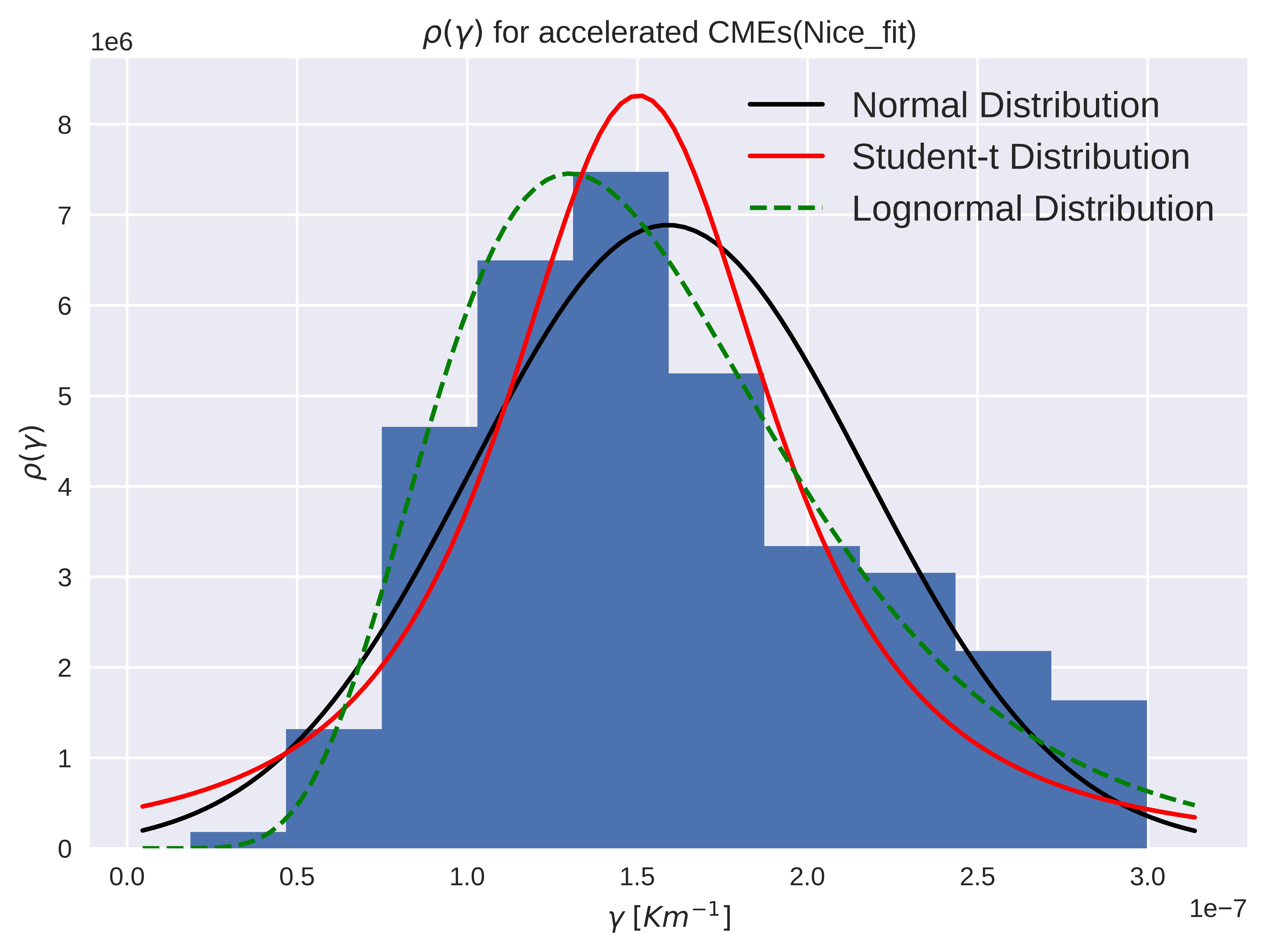
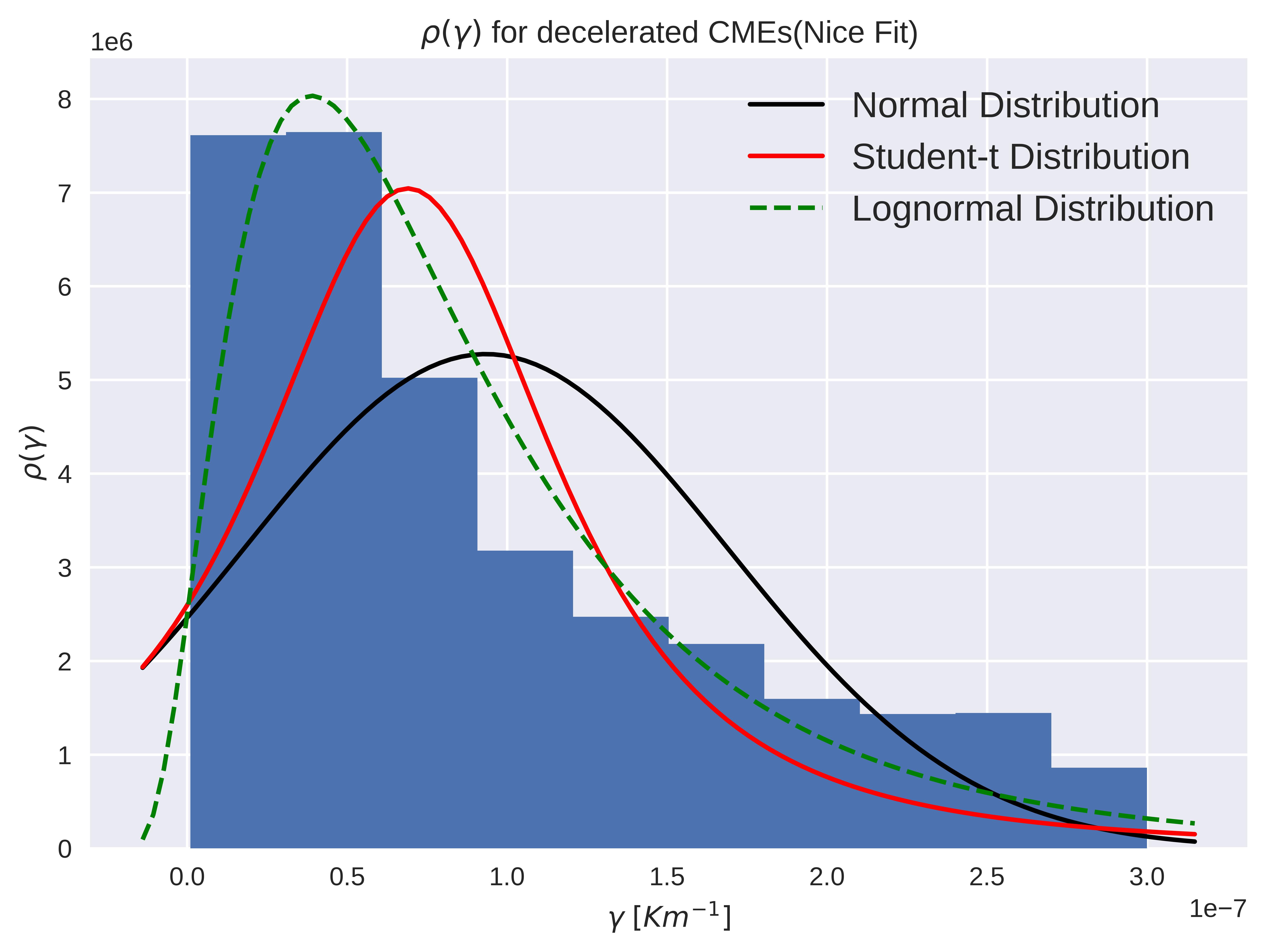
Figure 7: Probability distribution functions for drag parameters $\gamma$ for accelerated and decelerated CMEs. Left: $w$ PDFs for accelerated CMEs with Nice Fit label. Right: $w$ PDFs for decelerated CMEs with Nice Fit label.

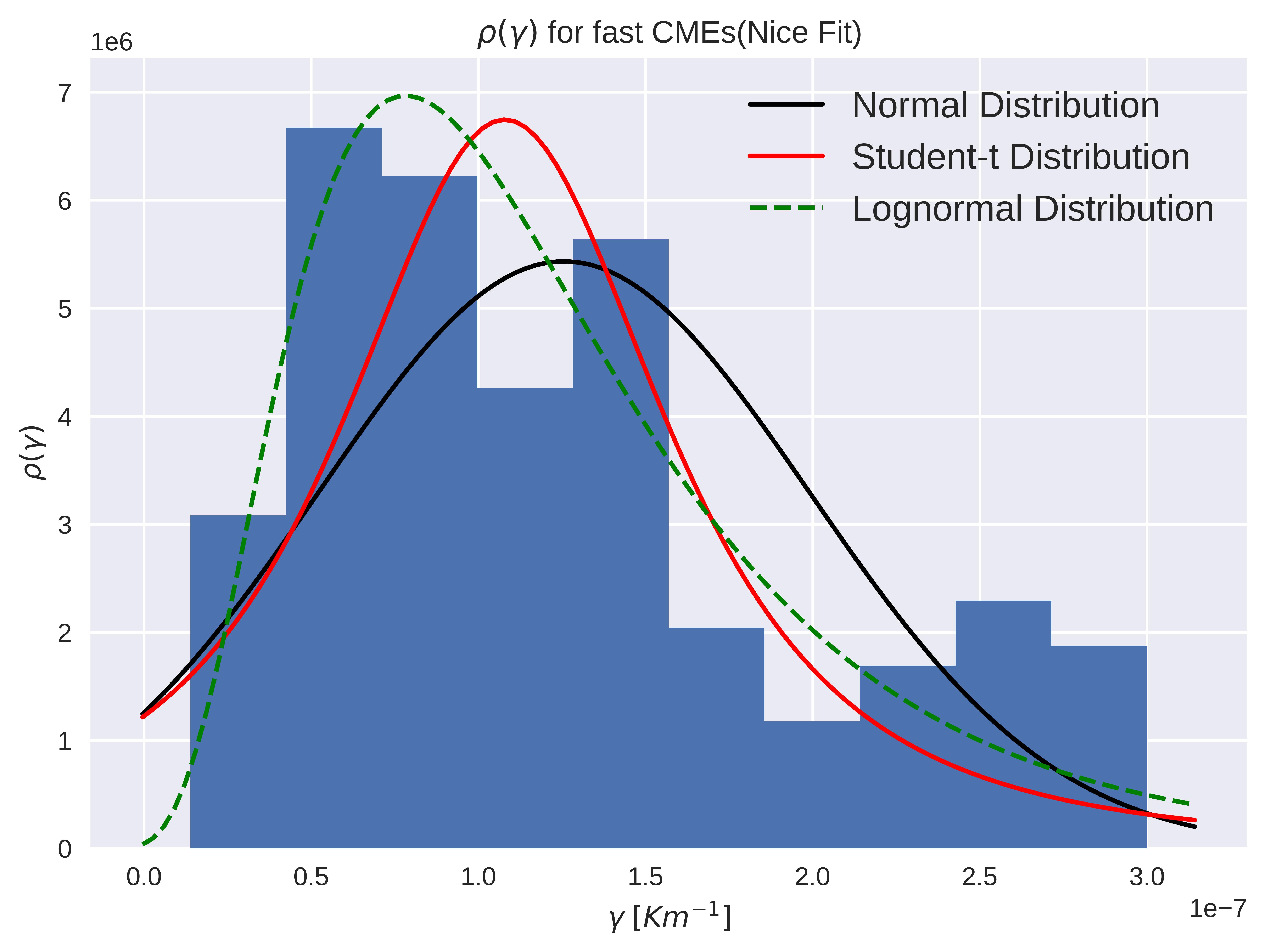
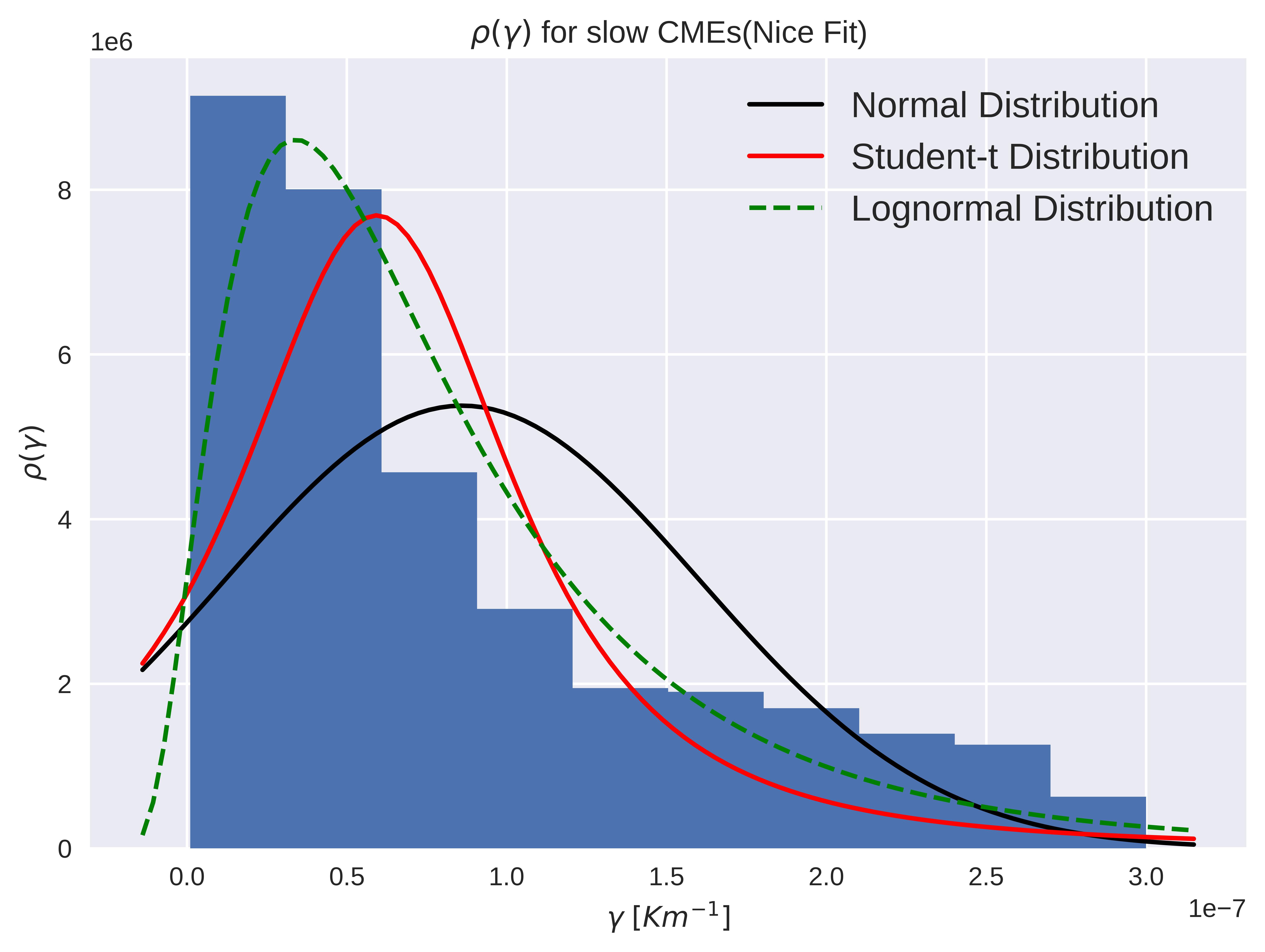
Figure 8: Probability distribution functions for drag parameters $\gamma$ for slow and fast CMEs. Left: $w$ PDFs for fast CMEs with Nice Fit label. Right: $w$ PDFs for slow CMEs with Nice Fit label.

Table 3: Parameter for different PDFs used to model drag parameter distribution. For the Lognormal function, tabulated values can not be used directly as average and standard deviation. The transformation from the fitting parameters to values used in the model can be done by the equation 10.

CME Group	PDF	$\bar{\gamma}[Km^{-1}]$	$\sigma_{\gamma}[Km^{-1}]$	Args	RSS
Accelerated	Normal	1.590$\times 10^{-7}$	5.793$\times 10^{-8}$	-	2.528$\times 10^{13}$
	Student’s-t	1.503$\times 10^{-7}$	4.247$\times 10^{-8}$	1.988	2.490$\times 10^{13}$
	Lognormal	-15.642	0.354	-1.186$\times 10^{-8}$	6.385$\times 10^{12}$
Decelerated	Normal	9.339$\times 10^{-08}$	7.562$\times 10^{-08}$	-	1.089$\times 10^{15}$
	Student’s-t	6.899$\times 10^{-08}$	5.016$\times 10^{-08}$	1.988	8.029$\times 10^{14}$
	Lognormal	-16.178	0.652	0.6518	2.723$\times 10^{14}$
Slow	Normal	8.609$\times 10^{-08}$	7.419$\times 10^{-08}$	-	1.519$\times 10^{15}$
	Student’s-t	5.936$\times 10^{-08}$	4.595$\times 10^{-08}$	1.988	1.010$\times 10^{15}$
	Lognormal	-16.252	0.658	-2.276$\times 10^{-08}$	4.034$\times 10^{14}$
Fast	Normal	1.256$\times 10^{-07}$	7.342$\times 10^{-08}$	-	5.319$\times 10^{14}$
	Student’s-t	1.079$\times 10^{-07}$	5.238$\times 10^{-08}$	1.988	4.749$\times 10^{14}$
	Lognormal	-15.884	0.518	-1.838$\times 10^{-08}$	2.575$\times 10^{14}$

4 Discussion and Conclusions

The collection of CME-ICME pairs published in Napoletano et al. (2022) has been improved by the inclusion of DBM simulation data, PDF fitting parameters, and various other significant variables related to each individual CME-ICME occurrence. By quantifying the success rate of the DBM inversion procedure, we were able to identify a subset of CME-ICME pairs that are well described by the DBM during their heliospheric propagation and added to the dataset the information about such categorization of CME events. This kind of categorization delivers a lot of promise for the space weather community, as it can provide significant insights into the circumstances that make the DBM approximation fail to predict the transit time for a CME event. On the other hand, those CME events where the DBM approximation is very valid can contribute to providing information about the model parameters $w$ and $\gamma$. It is worth mentioning that the version of DBM we used does not consider the CME geometry, with a very simple CME front described as a spherical shell centred on the Sun. Thus, all the CME-ICME entries that do not follow the DBM hypothesis deserve even further investigation, since we cannot tell if a ’no solution’, a ’poor’ or a ’bad’ label actually comes from a possible error in the initial CME-ICME association, a shortage in the geometrical description of the ICME, or something happening during the ICME propagation that cannot be described by the DBM (e.g. a CME-CME interaction). This, however, would require a thorough analysis of every single ICME and is beyond the scope of this work and may be the subject of a different work. The revised CME-ICME collection we are presenting also includes additional details such as the solar wind speed conditions experienced by propagating CME events, more parameters about the validation of the DBM hypothesis, and information about the acceleration or deceleration mechanisms during their propagation. The list of the improvements over the previous version published by Napoletano et al. (2022) are summarised in table 4. The revised dataset compiled and used in this work has been published at https://zenodo.org/record/8063404 and a description of its columns is also provided in the appendix A.

As just mentioned, the subset of events where the DBM approximation holds can be employed to extract the $\gamma$ and $w$ parameters of the DBM via a Monte Carlo-like inversion procedure. In this statistical study, we consider the uncertainties associated with the measure and the observation and incorporate them as input for the model and we only consider those CME events with more than 50% acceptance rate in the inversion procedure. The reason behind this criterion is to ensure that the CME propagation is modeled by DBM with enough confidence.

We have retrieved $\gamma$ and $w$ for 204 out of 213 ICMEs, which enables us to obtain robust statistics. The empirical PDF for the solar wind $w$ is modeled using two separate distributions for slow and fast solar wind conditions respectively with a threshold value of $w=500$ km/s for the fast solar wind. In Dumbović et al. (2018), Dumbović et al. (2021), Napoletano et al. (2018) and Napoletano et al. (2022), a Gaussian distribution is assumed as input PDF for $w$. Here, we have used the threshold of $w=500$ km/s for the fast solar wind speed, therefore, a normal distribution is no longer the ideal PDF. With this new threshold, the Student’s t-distribution is the best choice for most CME events. This latter finding is also supported by fitting PDFs for $w$ in a single CME approach. In Figure 9, a histogram of the most suitable PDFs for $w$ in individual CMEs approach is shown. Here, the Student’s t-distribution is strongly biased by the fact of hard thresholding and the RSS values of Student’s-t and normal distribution are fairly comparable, we therefore prefer the Gaussian PDF for the solar wind $w$.

The PDF for $\gamma$ is up for discussion from the previous works of Napoletano et al. (2018), Napoletano et al. (2022) and Dumbović et al. (2018),Dumbović et al. (2021), Čalogović et al. (2021). One group employs a lognormal function, while the other group uses a Gaussian Function as input PDF. We have tried to fit the PDF on the entire dataset and single CME events, and our study has provided light on the preference for these two different functions. From table 3, it is clear that lognormal distribution is the most favourable PDF as the RSS value is lower among other PDFs. On the contrary, when searching for the most suitable PDF in the single CME approach, the Gaussian PDF seems to be the best. In Figure 9, a histogram of the most suitable PDFs for $\gamma$ in individual CME approach is shown. A possible reason behind this discrepancy is the extensive dataset. Here, we have a used very large dataset of CME, which covers different ranges of mass and cross-sections of CME, also including almost two solar cycles’ length of CME events resulting in several kinds of solar wind density fluctuations in CME propagation. The inclusion of all these background parameters in fitting a PDF through a dataset leads to the long-tailed lognormal function since the $\gamma$-parameter is a quantitative measure of the drag efficiency that depends on many factors such as the mass and the cross-section of the CME, and on the solar wind density (Vršnak et al., 2013).

The refined dataset and the updated method presented in this work allowed us to explore a larger part of the $w-\gamma$ parameter space of the P-DBM model, including extreme values. We have investigated the possibility of $\gamma$ being a function of the ICME kinematic properties (i.e., accelerating or decelerating) or the solar wind properties (i.e., fast or slow). While there seems to be some difference between accelerating or decelerating ICME (see table 3 and Figure 7), the statistics need to be more robust to draw strong conclusions.

We suggest that our result and in particular, the revised CME-ICME list will benefit the space weather community since it will provide a test bench to compare how well we can predict CME arrival time and impact. Also, the associated information to every CME-ICME entry can help improve the accuracy and precision of other CME propagation models by including other relevant parameters. For example, a future plan of ours is to develop a Markov Chain Monte Carlo (MCMC) approach to further constrain the PDF for $w$ and $\gamma$. This catalogue’s new entries are expected to play a relevant part in this work, promoting the convergence of Markov chains and boosting the performance of our strategy.

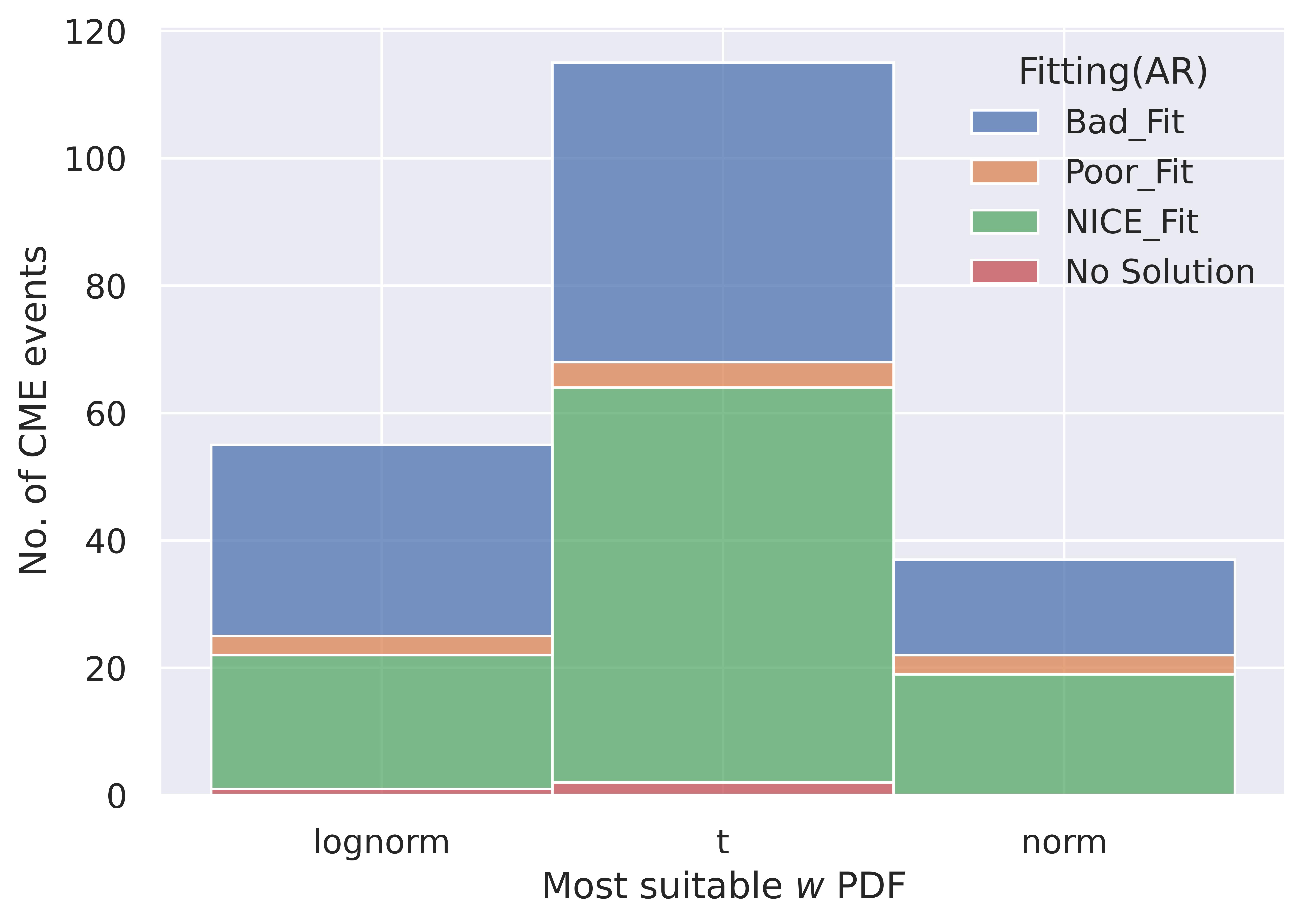
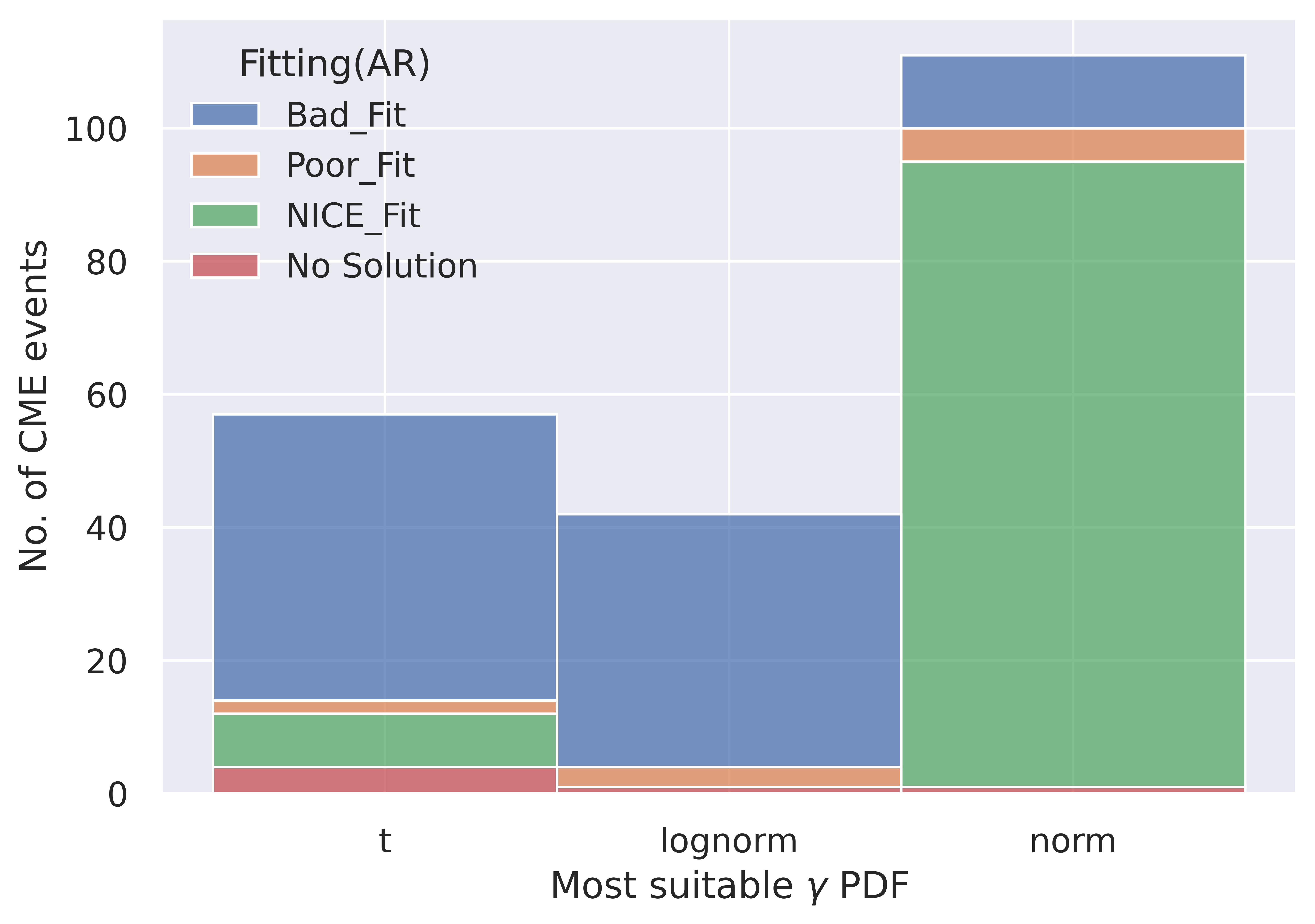
Figure 9: Histogram illustrating most suitable PDF for solar wind speed $w$ and drag parameter $\gamma$ in single CME approach. Within each PDF, various types of CME events are stratified and effectively stacked on top of one another.

Data Availability Statement: The ICME catalogue built as a part of this work along with data visualisation and PDF analysis modules for implementing DBM inversion procedure can be downloaded from https://zenodo.org/record/8063404 (Mugatwala et al., 2023).

Appendix A Description of revised data set.

As mentioned above, DBM inversion procedure requires initial position $r_{0}$, target position $r_{1AU}$, transit time $t_{1AU}$, initial speed $v_{0}$ and arrival speed $v_{a}$ to obtain $w$ and $\gamma$. For the purpose of this work, we have used the CME-ICME dataset from the Napoletano et al. (2022). This dataset contains all the required input quantities for the DBM inversion procedure. This dataset consists of 213 CME-ICME pairs from the year 1997 to 2018, which cover a time span of two solar cycles 23 and 24. In this dataset, information about the kinematic properties of CMEs at launch time was retrieved from the SOHO/LASCO CME Catalog . While arrival time and speed of the related ICMEs have been obtained from the Richardson and Cane (2010).

As mentioned in section 2.2, the uncertainty associated with different quantities is included in the inversion procedure. SOHO/LASCO catalogue provides CME speed in the plane of sky (POS) but to make a DBM forecast more accurate de projected speed has been used in the calculation. De projected radial speed has been obtained using equation 1 of Gopalswamy (2009). A more detailed explanation is given in appendix A2 of Napoletano et al. (2022). Associated solar wind speed type (column: SW_type) for each event is hypothesised by determining the presence of a coronal hole close to the CME source region (see appendix A3 of Napoletano et al. (2022))

The Description of different columns in the database and their source work is provided in a table 4

Table 4: Column description of the ICME dataset created as a part of this work

Name Keyword Description Source LASCO Start LASCO_Start First CME appearance in LASCO C2/C3 coronagraphs LASCO/CDAW Start Date Start_Date Time when CME reaches to 20 R$\odot$ Napoletano et al. (2022) Arrival Date Arrival_Date Estimated arrival time of ICME using insitu signatures R & C Plasma Event Duration PE_duration End of ICME plasma signatures after col 3 is recorded R & C Arrival Speed Arrival_v ICME arrival speed at L1 (km/s) R & C Transit Time Transit_time (hrs) Computed between col 1 and col 3 Napoletano et al. (2022) Transit Time Error Transit_time_err (hrs) Error associated to the start date of CME Napoletano et al. (2022) LASCO date LASCO_Date Most likely associated CME observed by LASCO LASCO/CDAW LASCO speed LASCO_v (km/s) speed correspond to the fastest moving point of CME in LASCO FOV LASCO/CDAW Position Angle LASCO_pa (deg) Counterclockwise (from solar North) angle of appearance into coronographs LASCO/CDAW Angular Width LASCO_da (deg.) Angular expansion of CME into coronographs LASCO/CDAW Halo LASCO_halo If LASCO_da is $>$270° then ’FH’ (full halo), if $>$180° ’HH’ (half halo), if $>$90° ’PH’(partial halo), otherwise ’NO LASCO/CDAW De- Projected Speed v_r (km/s) De-projected CME speed Napoletano et al. (2022) De- Projected Speed Error v_r_err (km/s) Uncertainty of CME initial speed Napoletano et al. (2022) Theta Source Theta_source (arcsec) Longitude of the most likely source of CME Napoletano et al. (2022) Phi Source Phi_source (arcsec) Co-latitude of the most likely source of CME Napoletano et al. (2022) Source POS error source_err (deg.) Uncertainty of the most likely CME source Napoletano et al. (2022) POS source angle POS_source_angle (deg.) Principal angle of the most likely CME source Napoletano et al. (2022) Relative width rel_wid (rad.) De-projected width of CME Napoletano et al. (2022) Mass Mass (gm) Estimated CME Mass LASCO/CDAW Solar Wind Type(CH) SW_type Solar wind (slow, S, or fast, F) interacting with the ICME based on the presence of coronal hole near CME location Napoletano et al. (2022) Bz Bz (nT) z-component of magnetic field at L1 and CME arrival time R & C Dst DST Geomagnetic Dst index recorded at CME arrival R & C Statistical de projected speed v_r_stat (km/s) Statistical de-projected CME speed, that is, $v\_r\_stat=LASCO\_v*1.027+41.5$ Acceleration Accel. (m/s 2) Residual acceleration at last CME observation Napoletano et al. (2022) Analytical Wind Analyitic_w (km/s) solar wind from DBM exact inversion Napoletano et al. (2022) Analytical gamma Analyitic_gamma (km^-1) drag parameter, $\gamma$, from DBM exact inversion Napoletano et al. (2022) Transit Time (Simulated) T1_Sim (hrs) Transit time calculated using P-DBM This Work Transit Time error (Simulated) T1_Sim_err (hrs) error associated with transit time in P-DBM This Work Impact Speed (Simulated) V1_Sim (km/s) calculated CME arrival speed using P-DBM This Work Impact Speed error (Simulated) V1_Sim_err (km/s) error associated with arrival speed in P-DBM This Work Solar Wind Speed W_Sim (km/s) Mean value of solar wind speed from inversion procedure This Work Solar Wind Speed Error W_Sim_err (km/s) Standard deviation of solar wind speed from inversion procedure This Work Gamma Simulated Gamma_Sim_s (km^-1) ’s’ parameter for lognormal PDF This Work Gamma Error Simulated Gamma_Sim_loc (km^-1) ${}^{\prime}loc^{\prime}$ parameter for lognormal PDF This Work Gamma Simulated (log) Gamma_Sim_scale ${}^{\prime}scale^{\prime}$ parameter for lognormal PDF This Work Optimal Transit Time T1_opt Minimally deviated transit time compared to observed one This Work Optimal Impact Speed V1_opt V1 correspond to T1_opt This Work Optimal W W_opt W correspond to T1_opt This Work Optimal gamma Gamma_opt gamma correspond to T1_opt This Work Optimal V_r V_r_opt V_r correspond to T1_opt This Work W CI min W99_min minimum value of 99% confidence interval for w This Work W CI max W99_max maximum value of 99% confidence interval for w This Work Gamma CI min Gamma99_min minimum value of 99% confidence interval for gamma This Work Gamma CI max Gamma99_max maximum value of 99% confidence interval for gamma This Work CME Type (V_r_opt) CME_type CME type based on W_sim (Accelerating/ Decelerating ) This Work CME Type (V_r) CME_type_v0 CME type based on W_opt (accelerating: A/ decelerating D) This Work Solar wind Type (Wth) Wind_type Solar wind (based on threshold value) interacting with ICME This Work Target distance R1(AU) (AU) Sun-Earth Distance at CME start date (Col2) This Work Fitting Fitting(AR) Goodness of Inversion procedure: Nice / Poor / Bad This Work Acceptance Rate Acceptance_Rate Acceptance rate of inversion procedure This Work Best W PDF Best_fit_W Most suitable PDF for W This Work Best gamma PDF Best_fit_gamma Most suitable PDF for gamma This Work

Appendix B Mathematical description of Lognormal Distribution

To find the parameters of lognormal PDF we have used a python package named distfit Taskesen (2023) which relies on SciPy Virtanen et al. (2020). The standardized form of lognormal function is given as:

$$f(x,s)=\frac{1}{sx\sqrt{2\pi}}\exp(\frac{-\ln^{2}x}{2s^{2}})$$ (7)

To shift and/or scale the above distribution function, SciPy or distfit use two more input parameters namely loc and scale. With these 2 more parameters, the new function will be:

$$f(x,s,loc,scale)=\frac{f(y,s)}{scale}$$ (8)

where $y=\frac{x-loc}{scale}$. Suppose, a variable X is following a normal distribution with parameters $\mu$ and $\sigma$. Then, lognormally distributed variable Y=$exp$(X) has $\mu$ = $ln(scale)$ and $\sigma=s$. The simplified version of formula 8 is given as follow:

$$f(x,s,loc,scale)=\frac{1}{s(x-loc)\sqrt{2\pi}}exp\left[-\bigg{(}\frac{(ln(x-loc)-\mu)}{\sqrt{2}s}\bigg{)}^{2}\right]$$ (9)

while a lognormal function used by Napoletano et al. (2018) is

$$f(x,)=\frac{1}{s\sqrt{2\pi}}exp\left[-\bigg{(}\frac{(lnx-\mu)}{\sqrt{2}s}\bigg{)}^{2}\right]$$ (10)

References

- Aquino and Sreeja (2013) Aquino, M., and V. Sreeja, 2013. Correlation of scintillation occurrence with interplanetary magnetic field reversals and impact on Global Navigation Satellite System receiver tracking performance. Space Weather, 11(5), 219–224. Https://doi.org/10.1002/swe.20047.
- Barbieri and Mahmot (2004) Barbieri, L., and R. Mahmot, 2004. October–November 2003’s space weather and operations lessons learned. Space Weather, 2(9). Https://doi.org/10.1029/2004SW000064.
- Bobra and Ilonidis (2016) Bobra, M. G., and S. Ilonidis, 2016. Predicting coronal mass ejections using machine learning methods. The Astrophysical Journal, 821(2), 127. 10.3847/0004-637X/821/2/127.
- Brueckner et al. (1995) Brueckner, G., R. Howard, M. Koomen, C. Korendyke, D. Michels, et al., 1995. The large angle spectroscopic coronagraph (LASCO) visible light coronal imaging and spectroscopy. The SOHO mission, 357–402. Https://doi.org/10.1007/BF00733434.
- Čalogović et al. (2021) Čalogović, J., M. Dumbović, D. Sudar, B. Vršnak, K. Martinić, M. Temmer, and A. M. Veronig, 2021. Probabilistic Drag-Based Ensemble Model (DBEM) Evaluation for Heliospheric Propagation of CMEs. Solar Physics, 296(7). 10.1007/s11207-021-01859-5.
- Camporeale (2019) Camporeale, E., 2019. The challenge of machine learning in space weather: Nowcasting and forecasting. Space Weather, 17(8), 1166–1207. Https://doi.org/10.1029/2018SW002061.
- Cargill (2004) Cargill, P. J., 2004. On the Aerodynamic Drag Force Acting on Interplanetary Coronal Mass Ejections. Solar Physics, 221(1), 135–149. 10.1023/b:sola.0000033366.10725.a2.
- Chen (2011) Chen, P., 2011. Coronal mass ejections: models and their observational basis. Living Reviews in Solar Physics, 8, 1–92. Https://doi.org/10.12942/lrsp-2011-1.
- Del Moro et al. (2019) Del Moro, D., G. Napoletano, R. Forte, L. Giovannelli, E. Pietropaolo, and F. Berrilli, 2019. Forecasting the 2018 February 12th CME propagation with the P-DBM model: A fast warning procedure. Ann Geophys, 61. Https://dx.doi.org/10.4401/ag-7750.
- Domingo et al. (1995) Domingo, V., B. Fleck, and A. I. Poland, 1995. The SOHO Mission: an Overview. Solar Physics, 162, 1–37. 10.1007/BF00733425.
- Dumbović et al. (2021) Dumbović, M., J. Čalogović, K. Martinić, B. Vršnak, D. Sudar, M. Temmer, and A. Veronig, 2021. Drag-based model (DBM) tools for forecast of coronal mass ejection arrival time and speed. Frontiers in Astronomy and Space Sciences, 8, 639,986. Https://doi.org/10.3389/fspas.2021.639986.
- Dumbović et al. (2018) Dumbović, M., J. Čalogović, B. Vršnak, M. Temmer, M. L. Mays, A. Veronig, and I. Piantschitsch, 2018. The Drag-based Ensemble Model (DBEM) for Coronal Mass Ejection Propagation. The Astrophysical Journal, 854(2), 180. 10.3847/1538-4357/aaaa66.
- Eyles et al. (2009) Eyles, C., R. Harrison, C. J. Davis, N. Waltham, B. Shaughnessy, et al., 2009. The heliospheric imagers onboard the STEREO mission. Solar Physics, 254(2), 387–445. Https://doi.org/10.1007/s11207-008-9299-0.
- Gopalswamy (2009) Gopalswamy, N., 2009. Coronal mass ejections and space weather. In Climate and Weather of the Sun-Earth System (CAWSES): Selected Papers from the 2007 Kyoto Symposium, 77–120. Terrapub Tokyo, Japan. Http://www.terrapub.co.jp/onlineproceedings/ste/CAWSES2007/index.html.
- Gopalswamy et al. (2000) Gopalswamy, N., A. Lara, R. P. Lepping, M. L. Kaiser, D. Berdichevsky, and O. C. St. Cyr, 2000. Interplanetary acceleration of coronal mass ejections. Geophysical Research Letters, 27(2), 145–148. Https://doi.org/10.1029/1999GL003639, https://agupubs.onlinelibrary.wiley.com/doi/pdf/10.1029/1999GL003639, URL https://agupubs.onlinelibrary.wiley.com/doi/abs/10.1029/1999GL003639.
- Gosling et al. (1991) Gosling, J., D. McComas, J. Phillips, and S. Bame, 1991. Geomagnetic activity associated with Earth passage of interplanetary shock disturbances and coronal mass ejections. Journal of Geophysical Research: Space Physics, 96(A5), 7831–7839. 10.1029/91JA00316.
- Howard et al. (2008) Howard, R. A., J. D. Moses, A. Vourlidas, J. S. Newmark, D. G. Socker, et al., 2008. Sun Earth Connection Coronal and Heliospheric Investigation (SECCHI). Space Science Reviews, 136(1-4), 67–115. 10.1007/s11214-008-9341-4.
- Ivezić et al. (2014) Ivezić, Ž., A. J. Connolly, J. T. VanderPlas, and A. Gray, 2014. Statistics, data mining, and machine learning in astronomy. In Statistics, Data Mining, and Machine Learning in Astronomy. Princeton University Press. Https://doi.org/10.1515/97814008489110.
- Kaiser et al. (2008) Kaiser, M. L., T. A. Kucera, J. M. Davila, O. C. St. Cyr, M. Guhathakurta, and E. Christian, 2008. The STEREO Mission: An Introduction. Space Science Reviews, 136, 5–16. 10.1007/s11214-007-9277-0.
- Koskinen and Huttunen (2006) Koskinen, H., and K. Huttunen, 2006. Geoeffectivity of coronal mass ejections. Space Science Reviews, 124, 169–181. Https://doi.org/10.1007/s11214-006-9103-0.
- Koskinen and Huttunen (2007) Koskinen, H., and K. Huttunen, 2007. Geoeffectivity of coronal mass ejections. Solar Dynamics and Its Effects on the Heliosphere and Earth, 169–181. Https://doi.org/10.1007/s11214-006-9103-0.
- Liu et al. (2018) Liu, J., Y. Ye, C. Shen, Y. Wang, and R. Erdélyi, 2018. A new tool for CME arrival time prediction using machine learning algorithms: CAT-PUMA. The Astrophysical Journal, 855(2), 109. 10.3847/1538-4357/aaae69.
- Liu et al. (2010) Liu, Y., A. Thernisien, J. G. Luhmann, A. Vourlidas, J. A. Davies, R. P. Lin, and S. D. Bale, 2010. Reconstructing coronal mass ejections with coordinated imaging and in situ observations: Global structure, kinematics, and implications for space weather forecasting. The Astrophysical Journal, 722(2), 1762. Http://dx.doi.org/10.1088/0004-637X/722/2/1762.
- Manchester et al. (2017) Manchester, W., E. K. Kilpua, Y. D. Liu, N. Lugaz, P. Riley, T. Török, and B. Vršnak, 2017. The physical processes of CME/ICME evolution. Space Science Reviews, 212, 1159–1219. Https://doi.org/10.1007/s11214-017-0394-0.
- Manoharan (2006) Manoharan, P., 2006. Evolution of coronal mass ejections in the inner heliosphere: A study using white-light and scintillation images. Solar physics, 235, 345–368. Https://doi.org/10.1007/s11207-006-0100-y.
- Mugatwala et al. (2023) Mugatwala, R., S. Chierichini, G. Francisco, G. Napoletano, R. Foldes, L. Giovannelli, G. D. Gasperis, E. Camporeale, R. Erdélyi, and D. D. Moro, 2023. Wolpes11/PDBM-project-for-ICMEs. 10.5281/zenodo.8063404, URL https://doi.org/10.5281/zenodo.8063404.
- Napoletano et al. (2022) Napoletano, G., R. Foldes, E. Camporeale, G. de Gasperis, L. Giovannelli, E. Paouris, E. Pietropaolo, J. Teunissen, A. K. Tiwari, and D. D. Moro, 2022. Parameter Distributions for the Drag-Based Modeling of CME Propagation. Space Weather, 20(9). 10.1029/2021sw002925.
- Napoletano et al. (2018) Napoletano, G., R. Forte, D. D. Moro, E. Pietropaolo, L. Giovannelli, and F. Berrilli, 2018. A probabilistic approach to the drag-based model. Journal of Space Weather and Space Climate, 8, A11. 10.1051/swsc/2018003.
- Odstrcil et al. (2003) Odstrcil, D., M. Vandas, V. J. Pizzo, and P. MacNeice, 2003. Numerical simulation of interacting magnetic flux ropes. In AIP Conference Proceedings, vol. 679, 699–702. American Institute of Physics. Https://doi.org/10.1063/1.1618690.
- Paouris and Mavromichalaki (2017) Paouris, E., and H. Mavromichalaki, 2017. Effective acceleration model for the arrival time of interplanetary shocks driven by coronal mass ejections. Solar Physics, 292, 1–11. Https://doi.org/10.1007/s11207-017-1212-2.
- Paouris et al. (2021) Paouris, E., J. Čalogović, M. Dumbović, M. L. Mays, A. Vourlidas, A. Papaioannou, A. Anastasiadis, and G. Balasis, 2021. Propagating Conditions and the Time of ICME Arrival: A Comparison of the Effective Acceleration Model with ENLIL and DBEM Models. Solar Physics, 296(1), 12. 10.1007/s11207-020-01747-4, URL https://doi.org/10.1007/s11207-020-01747-4.
- Papaioannou et al. (2016) Papaioannou, A., I. Sandberg, A. Anastasiadis, A. Kouloumvakos, M. K. Georgoulis, K. Tziotziou, G. Tsiropoula, P. Jiggens, and A. Hilgers, 2016. Solar flares, coronal mass ejections and solar energetic particle event characteristics. Journal of Space Weather and Space Climate, 6, A42. Https://doi.org/10.1051/swsc/2016035.
- Piersanti et al. (2017) Piersanti, M., T. Alberti, A. Bemporad, F. Berrilli, R. Bruno, et al., 2017. Comprehensive analysis of the geoeffective solar event of 21 June 2015: Effects on the magnetosphere, plasmasphere, and ionosphere systems. Solar Physics, 292, 1–56. Https://doi.org/10.1007/s11207-017-1186-0.
- Pomoell and Poedts (2018) Pomoell, J., and S. Poedts, 2018. EUHFORIA: European heliospheric forecasting information asset. Journal of Space Weather and Space Climate, 8, A35. Https://doi.org/10.1051/swsc/2018020.
- Pulkkinen (2007) Pulkkinen, T., 2007. Space weather: terrestrial perspective. Living Reviews in Solar Physics, 4, 1–60. Https://doi.org/10.12942/lrsp-2007-1.
- Richardson and Cane (2010) Richardson, I. G., and H. V. Cane, 2010. Near-Earth Interplanetary Coronal Mass Ejections During Solar Cycle 23 (1996–2009): Catalog andSummary of Properties. Solar Physics, 264(1), 189–237. 10.1007/s11207-010-9568-6, URL https://doi.org/10.1007/s11207-010-9568-6.
- Riley et al. (2018) Riley, P., M. L. Mays, J. Andries, T. Amerstorfer, D. Biesecker, et al., 2018. Forecasting the Arrival Time of Coronal Mass Ejections: Analysis of the CCMC CME Scoreboard. Space Weather, 16(9), 1245–1260. 10.1029/2018sw001962.
- Rollett et al. (2016) Rollett, T., C. Möstl, A. Isavnin, J. A. Davies, M. Kubicka, U. V. Amerstorfer, and R. A. Harrison, 2016. ElEvoHI: a novel CME prediction tool for heliospheric imaging combining an elliptical front with drag-based model fitting. The Astrophysical Journal, 824(2), 131. 10.3847/0004-637X/824/2/13.
- Sachdeva et al. (2015) Sachdeva, N., P. Subramanian, R. Colaninno, and A. Vourlidas, 2015. CME PROPAGATION: WHERE DOES AERODYNAMIC DRAG ”TAKE OVER” ? The Astrophysical Journal, 809(2), 158. 10.1088/0004-637x/809/2/158.
- Sachdeva et al. (2017) Sachdeva, N., P. Subramanian, A. Vourlidas, and V. Bothmer, 2017. CME Dynamics Using STEREO and LASCO Observations: The Relative Importance of Lorentz Forces and Solar Wind Drag. Solar Physics, 292(9), 118. 10.1007/s11207-017-1137-9, URL https://doi.org/10.1007/s11207-017-1137-9.
- Schrijver and Siscoe (2010) Schrijver, C. J., and G. L. Siscoe, 2010. Heliophysics: space storms and radiation: causes and effects. Cambridge University Press. 2010hssr.book…..S.
- Schwenn (2006) Schwenn, R., 2006. Space Weather: The Solar Perspective. Living Reviews in Solar Physics, 3. 10.12942/lrsp-2006-2.
- Shea and Smart (1998) Shea, M., and D. Smart, 1998. Space weather: The effects on operations in space. Advances in Space Research, 22(1), 29–38. Https://doi.org/10.1016/S0273-1177(97)01097-1.
- Sreeja (2016) Sreeja, V., 2016. Impact and mitigation of space weather effects on GNSS receiver performance. Geoscience letters, 3(1), 24.
- Taskesen (2023) Taskesen, E., 2023. Distfit is a python library for probability density fitting. 10.5281/zenodo.7650685, URL https://doi.org/10.5281/zenodo.7650685.
- Temmer (2021) Temmer, M., 2021. Space weather: the solar perspective. Living Reviews in Solar Physics, 18(1). 10.1007/s41116-021-00030-3.
- Tsurutani et al. (1988) Tsurutani, B. T., W. D. Gonzalez, F. Tang, S. I. Akasofu, and E. J. Smith, 1988. Origin of interplanetary southward magnetic fields responsible for major magnetic storms near solar maximum (1978–1979). Journal of Geophysical Research: Space Physics, 93(A8), 8519–8531. 10.1029/JA093iA08p08519.
- VanderPlas et al. (2012) VanderPlas, J., A. J. Connolly, Ž. Ivezić, and A. Gray, 2012. Introduction to astroML: Machine learning for astrophysics. In 2012 conference on intelligent data understanding, 47–54. IEEE. Https://doi.org/10.1109/CIDU.2012.6382200.
- Veettil et al. (2019) Veettil, S. V., C. Cesaroni, M. Aquino, G. De Franceschi, F. Berrili, et al., 2019. The ionosphere prediction service prototype for GNSS users. Journal of Space Weather and Space Climate, 9, A41. Https://doi.org/10.1051/swsc/2019038.
- Virtanen et al. (2020) Virtanen, P., R. Gommers, T. E. Oliphant, M. Haberland, T. Reddy, et al., 2020. SciPy 1.0: fundamental algorithms for scientific computing in Python. Nature methods, 17(3), 261–272. Https://dx.doi.org/10.1038/s41592-019-0686-2.
- Vourlidas et al. (2019) Vourlidas, A., S. Patsourakos, and N. P. Savani, 2019. Predicting the geoeffective properties of coronal mass ejections: current status, open issues and path forward. Philosophical Transactions of the Royal Society A: Mathematical, Physical and Engineering Sciences, 377(2148), 20180,096. 10.1098/rsta.2018.0096.
- Vršnak (2001) Vršnak, B., 2001. Dynamics of solar coronal eruptions. Journal of Geophysical Research: Space Physics, 106(A11), 25,249–25,259.
- Vršnak et al. (2004) Vršnak, B., D. Ruždjak, D. Sudar, and N. Gopalswamy, 2004. Kinematics of coronal mass ejections between 2 and 30 solar radii-What can be learned about forces governing the eruption? Astronomy & Astrophysics, 423(2), 717–728.
- Vršnak et al. (2013) Vršnak, B., T. Žic, D. Vrbanec, M. Temmer, T. Rollett, et al., 2013. Propagation of interplanetary coronal mass ejections: The drag-based model. Solar physics, 285(1-2), 295–315.
- Wang et al. (2019) Wang, P., Y. Zhang, L. Feng, H. Yuan, Y. Gan, S. Li, L. Lu, B. Ying, W. Gan, and H. Li, 2019. A new automatic tool for CME detection and tracking with machine-learning techniques. The Astrophysical Journal Supplement Series, 244(1), 9. 10.3847/1538-4365/ab340c.
- Webb and Howard (2012) Webb, D. F., and T. A. Howard, 2012. Coronal mass ejections: Observations. Living Reviews in Solar Physics, 9(1), 1–83. Https://doi.org/10.12942/lrsp-2012-3.
- Wu et al. (2007) Wu, C.-C., C. Fry, S. Wu, M. Dryer, and K. Liou, 2007. Three-dimensional global simulation of interplanetary coronal mass ejection propagation from the Sun to the heliosphere: Solar event of 12 May 1997. Journal of Geophysical Research: Space Physics, 112(A9). Https://doi.org/10.1029/2006JA012211.