Towards a general description of the cavitation threshold in acoustic systems

Abstract

Traditionally, the occurrence of cavitation has been related to the ratio between flow velocity and pressure gradient in the case of hydrodynamic cavitation, or some combination of vapor pressure and surface tension. However, both formulations present a large discrepancy with experimental data for cases in which cavitation is induced by acoustic waves. The present study aims to identify a more suitable cavitation threshold for such cases. The methodology adopted in this work consists of a combination of visualization with high-speed cameras and direct measurements using a hydrophone. The data collected confirmed that the vapor pressure is not a proper indicator of cavitation occurrence for an acoustic system characterized by high frequencies. The main reason behind the inability of vapor pressure to predict incipient cavitation in acoustic systems is that they evolve very quickly toward strong gradients in pressure, and the quasi-static assumptions used by traditional models are not valid. Instead, the system evolves towards a metastable state (Brennen, 2013), where the liquid exhibits an elastic behavior and can withstand negative pressures. A new cavitation number accounting for the tensile strength of the liquid was defined. An acoustic analogy is also proposed for the description, with the same framework, of an impulsive cavitation phenomenon.

Keywords Acoustic cavitation  $\cdot$ Impulsive cavitation  $\cdot$ Tensile strength  $\cdot$ Cavitation threshold

Cavitation induced by acoustic waves is a physical phenomenon used, nowadays, in a wide range of industrial processes and laboratory applications, from the pharmaceutical and clinical sector to biomass treatment and heavy oil upgrading (Guida et al., 2022; Sharma et al., 2003; Flores et al., 2021). Most applications are based on high-power ultrasound transducers to generate cavitation. In this type of system, vapor-filled cavities form as a consequence of the propagation of acoustic waves in a liquid domain (Suslick et al., 1999; Kozmus et al., 2022). Once formed, the vapor cavities oscillate, storing acoustic energy, until they finally collapse. In this way, the energy stored is deposited in confined regions of space. The confined energy release induces the formation of hot spots, characterized by high pressure and temperature (Suslick and Flannigan, 2008), and the production of radicals species (Sonochemistry) (Suslick, 1990; Didenko et al., 1999). The collapse of the vapor cavities also induces peculiar fluid dynamic phenomena, like shock waves and micro-jets (Wagterveld et al., 2011). These phenomena can potentially increase the reaction rate of various chemical processes, enhancing the mixing in a multi-phase system, or the fragmentation in a solution.

Laboratory and industrial processes, based on acoustic cavitation, are commonly carried out using a variety of ultrasound reactor designs, working frequencies, and operative conditions. However, it is not always clear what is the optimal combination of working parameters for a given process. To improve the design and the efficiency of these systems, it is crucial to understand the physical mechanism behind cavitation induced by acoustic waves, to be able to predict the cavitation onset (Smirnov et al., 2022). Traditionally, the cavitation threshold is established by considering that the phase transition occurs when pressure reaches the saturation pressure of the liquid medium. The most widely adopted Cavitation number ($Ca$) is defined similarly to the Euler number:

$$Ca=\frac{p_{r}-p_{v}}{\frac{1}{2}\rho v^{2}},$$ (1)

where $p_{r}$ is the reference pressure, $p_{v}$ is the vapor pressure of the liquid, $\rho$ is the liquid density, and $v$ is the local velocity of the flow. This number is used to characterize hydrodynamic cavitation phenomena (Brennen, 2011; Arndt, 1981). Recently, an alternative cavitation number, based on the vapor pressure as a cavitation threshold, has been introduced by Pan (Pan et al., 2017a). In this dimensionless number, the acceleration ($a$) and the depth of the liquid ($h$) appear as scaling factors:

$$Ca=\frac{p_{r}-p_{v}}{\rho ah},$$ (2)

The dimensionless number introduced by Pan et al. (2017a) can successfully predict cavitation phenomena in systems set into motion by an impulsive force. Fatjo (2016) introduced a similar dimensionless number for the prediction of cavitation in accelerated fluid.

While a cavitation number, based on the saturation vapor pressure, can describe certain phenomena effectively, it does not predict the onset of acoustic cavitation. Indeed, acoustic cavitation results from the propagation of sound waves in a liquid medium. The sound waves travel through the medium, generating compression and rarefaction regions. The fluid particles experience compressive deformation in the compression regime, generating a high-pressure region. On the contrary, where rarefaction occurs, the fluid particles are tensile deformed, with the consequent formation of low-pressure regions (Lurton, 2010). When the acoustic waves are characterized by high frequencies, the thermodynamic system evolves quickly, with strong gradients of the thermodynamic variables. Such a system is far from the theoretical hypothesis on which the definition of vapor pressure is based. Indeed, the theoretical framework and the experimental data used to build the phase diagrams, in the context of classical thermodynamics, are based on the assumption of a quasi-static process (Gyftopoulos and Beretta, 2005). A quasi-static process evolves sufficiently slowly to guarantee that the system remains in thermodynamic equilibrium at every instant of time (Woods, 1959; Moebs et al., 2016).

In a thermodynamic system where the quasi-static assumption is not valid, an isothermal depressurization may lead to a metastable state in which the liquid withstands pressures lower than the saturation pressure (Brennen, 2013), without turning into vapor. The pressure potentially reaches negative values with the liquid being in a state of tension (Brennen, 2013). Berthelot (1850) first attained this condition in a controlled environment in his work from 1850 demonstrating that purified water could withstand a tension of 50 atm before the “rupture”.

Brennen (2013) introduced an elastic analogy stating that liquids can behave like elastic media since they can withstand tension. The elastic property of liquids is described by the Deborah number ($De$), which is the ratio between the characteristic time for the self-diffusion of a molecule and the characteristic time of the applied force (Pelton et al., 2013; Noirez and Baroni, 2012; Urick, 1983). It is possible to define the Tensile Strength of a liquid as the maximum tensile stress (tension) that a liquid medium can withstand, while being ”stretched”, before changing phase to vapor. This theory supports the fact that the tensile strength, instead of the vapor pressure, should be considered as a cavitation threshold for the phenomena where the nucleation is induced by acoustic waves, especially at high frequencies, where the liquid increases its tendency to behave as an elastic medium. Furthermore, this leads us to consider that the tensile strength value should depend on the frequency of the acoustic wave.

In this regard, Urick (1983) proposed a direct dependency of the tensile strength on the frequency of the sound wave (Fig. 1). This dependency predicts a significant increase in the cavitation threshold of water as the frequency increases. The trend observed by Urick (1983) is justified by the occurrence of two mechanisms. The first one is the tendency of the liquid to increase its elastic response at a higher forcing frequency (high $De$ number). The second is related to the characteristic time of growth of a macroscopic bubble, starting from a nucleus. The chart, proposed by Urick (1983), is based on the experimental data of several authors. Esche (1952) measured the cavitation threshold of water at various frequencies. The shaded area, on the chart in Fig. 1, represents the range of observed values, while the dashed curve is the average estimated by Esche (1952). Strasberg (1959), using a forcing frequency of $25\text{\,}\mathrm{k}\mathrm{H}\mathrm{z}$, detected a cavitation threshold ranging from $2.5\text{\,}\mathrm{a}\mathrm{t}\mathrm{m}$ in tap water saturated with air to $6.5\text{\,}\mathrm{a}\mathrm{t}\mathrm{m}$ in degassed water (blue bar in Fig. 1). Blake (1949) measured values ranging from $3.5\text{\,}\mathrm{a}\mathrm{t}\mathrm{m}$ to $4.6\text{\,}\mathrm{a}\mathrm{t}\mathrm{m}$ for air-saturated and degassed water (orange bar in Fig. 1), using a frequency of $60\text{\,}\mathrm{k}\mathrm{H}\mathrm{z}$. The order of magnitude of these experimental values is lower than the value obtained in controlled environments, using highly purified liquids. Berthelot (1850) and Dixon (1909) obtained, respectively, values of $50\text{\,}\mathrm{b}\mathrm{a}\mathrm{r}$ and $200\text{\,}\mathrm{b}\mathrm{a}\mathrm{r}$, by using purified water. More recently, Caupin et al. (2012) obtained a cavitation pressure in the order of $-20\text{\,}\mathrm{M}\mathrm{P}\mathrm{a}$. However, these values, despite the controlled environment and the purified liquids, are far away from the theoretical limit established by the Homogeneous Nucleation Theory (Brennen, 2013), which predicts the rupture of pure water at values in the order of magnitude of $10^{4}$ atm. This discrepancy suggests that contaminants play a crucial role by decreasing the nucleation energy barrier, in every laboratory system and, in general, in real media (Brennen, 2013).

In the attempt to unify the theoretical understanding behind the onset of acoustic cavitation, we studied a system operating at $24\text{\,}\mathrm{k}\mathrm{H}\mathrm{z}$. A rigorous and repeatable methodology for defining the cavitation onset, from both visual and acoustic data, is defined. Furthermore, based on the experimental observation and on the Rayleigh analytical model(Rayleigh, 1896), a Cavitation Number is proposed (Viciconte et al., KAUST Research Repository, 15-06-2023). This dimensionless number contains the tensile strength as a cavitation threshold and the frequency, of the acoustic wave, as a scaling factor. Afterward, the same framework is applied, through an acoustic analogy, to a case of cavitation induced by impulsive motion (Pan et al., 2017a).

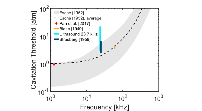
Figure 1: Experimental data of the cavitation threshold (tensile strength) as a function of the frequency. The data are related to measurements done by three authors: Esche (1952); Blake (1949); Strasberg (1959).

1 Experimental procedure

Cavitation inception, due to the propagation of ultrasound waves, in liquid water, has been widely investigated in an extensive experimental campaign. This section introduces a new methodology aimed at identifying the cavitation onset and measuring the acoustic pressure threshold. This is based on an analysis of data coming from high-speed imaging and the acoustic signal measured by a hydrophone. The experiments, aimed at identifying the cavitation onset and measuring the acoustic pressure threshold, have been conducted using the backlighting technique. A schematic illustration of the experimental setup is visible in Fig. 2. All the experiments were done using water with a temperature of 24^∘ C. The dissolved oxygen content (DO) of the liquid water was not altered with preliminary treatments. The experiments were conducted with a level of DO saturation percentage oscillating between 64% and 84%. A light (LED) source was placed on the back side of a water container and aligned with the axis of a cylindrical ultrasound probe (Hielscher UP400S, 400 W, 24 kHz), immersed in the liquid water (Fig. 2). The scene was captured using a high-speed camera (Photron FASTCAM Nova S16) at 200,000 fps (128x224 pixels). Seven different configurations have been tested during the experimental campaign. These configurations differ for the type of water, geometry and material of the transparent container, immersion depth of the probe, and the relative position between the probe and the hydrophone. More details about the experimental configurations can be found in the section Methodology.

The Displacement Amplitude ($A$) of the ultrasound probe (Hielscher UP400S) undergoes a transient state where it gradually increases over time, until reaching a steady state (Fig. 4). The high-speed camera was triggered, by the intensity of the hydrophone acoustic signal (AS-1 AQUARIAN Hydrophone) near cavitation inception. For measuring the pressure at which cavitation onset happens, the displacement of the probe has to be precisely measured. Since the displacement is in the order of magnitude of micrometers, an objective lens (10X magnification), providing a resolution of $1.98\text{\,}\mathrm{\SIUnitSymbolMicro}\mathrm{m}$/pixel, was used.

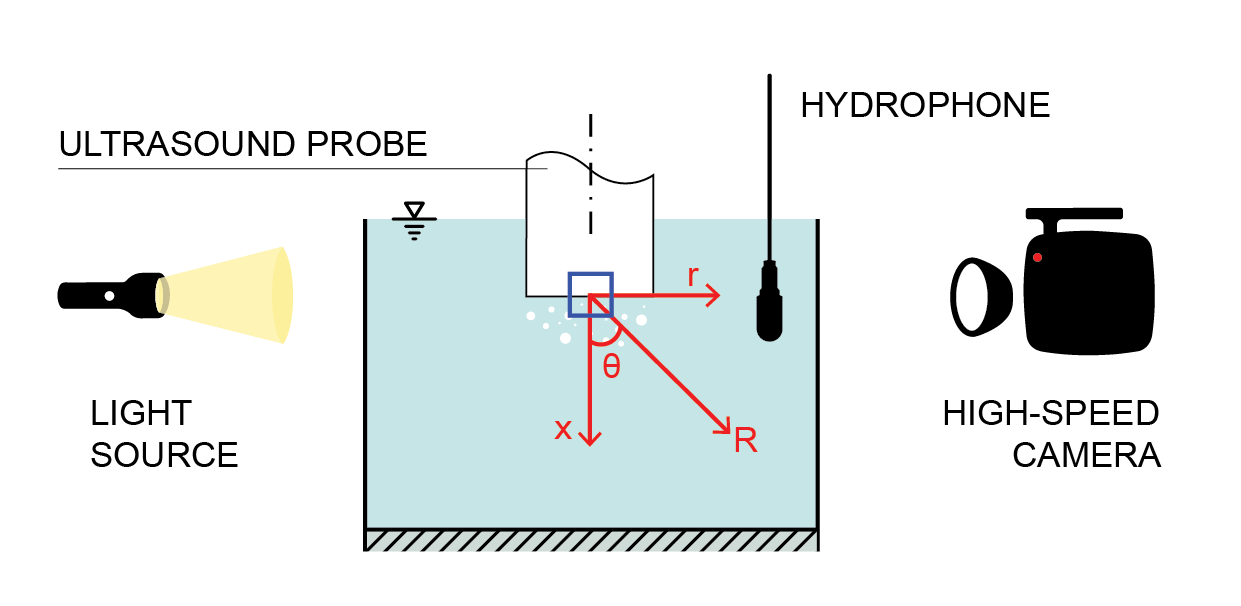
Figure 2: Schematic illustration of the backlighting setup utilized for the visualization experiments. The blue square indicates the portions of the domain framed by using the high-speed camera.

The sequence of images in Fig. 3 (A, B) shows the portion of the domain framed by the high-speed camera (blue outlined area in Fig. 2). The movement of the probe tip and the nucleation of the first vapor cavity are clearly visible. The cavitation onset, on the surface of the probe tip, is better observable by framing a wider region of the domain (Fig. 3 (C, D)). This has been done by using a Nikon MICRO Lens, having a focal length of $105\text{\,}\mathrm{m}\mathrm{m}$.

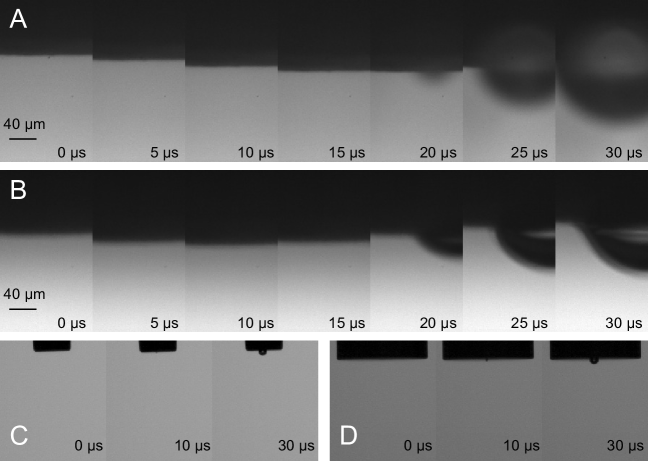
Figure 3: (A) Sequence of frames recorded by using the high-speed camera, coupled with a 10X objective lens. It is clearly visible the movement of the probe tip and the nucleation of the first cavity attached to the tip surface. This sequence is related to a 3 mm probe with a device nominal amplitude of 70 %. (B) Sequence of frames related to a 3 mm probe with a nominal amplitude of 100 %. (C) Sequence of images framed by using a Nikon MICRO Lens (105 mm). The nucleation of a cavity, attached to the surface, on the axis of a cylindrical probe (3 mm diameter) was captured. (D) Nucleation of a bubble on the tip surface of a cylindrical probe, having a diameter of 7 mm (recorded by using a 105 mm Nikon MICRO Lens).

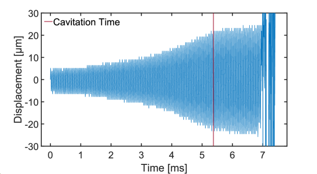
Figure 4: Result of the tracking procedure on one experimental observation (Conf. 3, Nominal Amplitude: 30 %). The blue function indicates the displacement of the probe over time, while the vertical red line represents the time at which cavitation happens.

The probe displacement was measured with a tracking procedure, implemented on Matlab Inc. (2022). Starting from the sequence of frames (Fig. 3 (A, B)), the displacement can be tracked by selecting one column of pixels and by taking the difference between adjacent pixels. The maximum value of the difference column defines the position of the probe tip at every time step. This can be used for tracking the movement over time until cavitation happens (Fig. 4). The Discrete Fourier Transform (DFT) of the data yields a probe frequency of $f_{p}=23.78$ kHz (close to the advertised value of the ultrasound device of 24 kHz). The red vertical line, in Fig. 4, at $5.2\text{\,}\mathrm{m}\mathrm{s}$ indicates the time of cavitation inception ($t_{cav}$), e.g. $20\text{\,}\mathrm{\SIUnitSymbolMicro}\mathrm{s}$ in Fig. 3.

The consistency of the cavitation time can be confirmed by the acoustic signal of the hydrophone (Fig. 5). A sudden change happens in correspondence to the cavitation time. The hydrophone signal is symmetric with respect to the zero, during the time lapse before cavitation occurs. This indicates that the information is only coming from the alternation of rarefaction and compression regions that characterize the propagation of ultrasound waves. After cavitation onset, the signal becomes asymmetric and chaotic (Fig. 5).

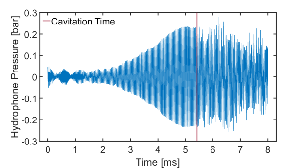
Figure 5: Acoustic pressure measured by the hydrophone (Conf. 3, Nominal Amplitude: 30 %). The vertical red line indicates the cavitation time defined with the visual tracking procedure.

The DFT frequency spectrum before and after cavitation are shown in Fig. 6. The frequency spectrum, related to the signal before cavitation happens (blue line in Fig. 6), shows peaks just at the vibration frequency of the ultrasound probe and at its multiples. Instead, the spectrum after cavitation (orange line in Fig. 6) has additional peaks and broad-band noise due to the presence of cavitation bubbles in the liquid domain.

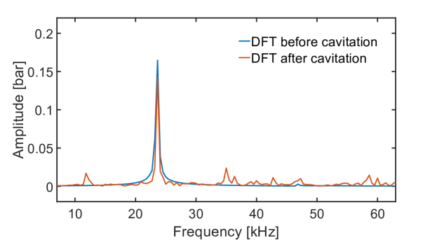
Figure 6: DFT frequency spectrum of the acoustic signal measured by the hydrophone. The blue line indicates the DFT spectrum before cavitation happens, while the orange line represents the spectrum after cavitation.

Once defined the cavitation time ($t_{cav}$), the Displacement Amplitude, at which cavitation happens ($A_{cav}$), was found by considering the nearest relative considering the nearest relative maxima and minima, in a neighborhood of $t_{cav}$ (red line in Fig. 4), and by averaging their absolute values. The procedure for finding $A_{cav}$ has been repeated for all experimental observations: for every one of the seven configurations, the Nominal Amplitude of the device ($A_{nom}$) has been varied four times (30%, 50%, 70%, and 100 % ). For every combination of parameters, the experimental run has been repeated at least two times. It is important to mention that after every run, the residual bubbles or cavities, have been carefully removed from the liquid domain and in particular from the surface of the probe tip. This was crucial to prevent the residual bubbles from acting as preferential cavitation sites in the next run. In the experimental configurations with the 3 mm worn ultrasound probe (Conf. 1, 2, 3) the minimum and the maximum value of ($A_{cav}$) are, respectively, $9.05\text{\,}\mathrm{\SIUnitSymbolMicro}\mathrm{m}$ (Conf. 3) and $36.71\text{\,}\mathrm{\SIUnitSymbolMicro}\mathrm{m}$ (Conf. 3). Instead, among the experimental configuration with the 3 mm new probe (Conf. 5, 6, 7), the minimum and the maximum value of the cavitation amplitude are $23.56\text{\,}\mathrm{\SIUnitSymbolMicro}\mathrm{m}$ (Conf. 5) and $67.19\text{\,}\mathrm{\SIUnitSymbolMicro}\mathrm{m}$ (Conf. 5).

2 Application of the Analytical Model and Results

Starting from the vibration frequency of the probe ($f$) and the displacement amplitude ($A$), the acoustic pressure field, generated by a flat acoustic transducer, can be analytically estimated by solving the equation introduced by Rayleigh, known as Rayleigh Integral (Rayleigh, 1896; Sherman and Butler, 2007;2011;; Kinsler et al., 2000). The Rayleigh’s formulation is based on the linear form of the Navier-Stokes Equations, where the advection term (non-linear) is neglected. This hypothesis is generally reasonable in acoustic since the velocity magnitude of the fluid particles of a sound wave is much smaller than the acceleration term (Pan et al., 2017b; Antkowiak et al., 2007). The gravitational and viscous terms can be also neglected in the Momentum Equations. Furthermore, the acoustic analytical solution is based on the No-Slip boundary condition, enforced between the flat surface of the transducer and the adjacent liquid medium (Rayleigh, 1896; Sherman and Butler, 2007;2011;; Kinsler et al., 2000).

The cylindrical probe (Fig. 2), used for the present experimental campaign, can be modeled by considering its analogy with acoustic radiation problem from a Plane Circular Piston (Rayleigh, 1896; Sherman and Butler, 2007;2011;; Kinsler et al., 2000). Assuming uniform velocity across the entire emitting flat surface, the Rayleigh integral can be analytically solved for the most relevant points of the acoustic field. An analytical solution can be obtained for the far-field and the near-field, along the axis of the probe (Sherman and Butler, 2007;2011;; Kinsler et al., 2000).

The solution of the near-field is crucial for investigating the cavitation phenomena. The point of the domain with the maximum absolute value of acoustic pressure ($p$) lies in the near-field, on the axis of the probe (Sherman and Butler, 2007;2011;; Kinsler et al., 2000); due to the axial symmetry of the circular transducer configuration. Assuming a cylindrical coordinate system, with radial coordinate $r$ and axial coordinate $x$ (Fig. 2), the complex acoustic pressure in the near-field, on the axis of the probe, $p(r=0,x,t)$, can be found by direct integration of the Rayleigh integral (Sherman and Butler, 2007;2011;; Kinsler et al., 2000):

$$p(r=0,x,t)=-\rho cv_{0}\left[e^{-ik\sqrt{(d^{2}+x^{2})}}-e^{-ikx}\right]e^{i\omega t},$$ (3)

where $i$ is the imaginary unit, $t$ is the time variable, $\rho$ and $c$ are respectively density and speed of sound of the liquid medium, $v_{0}$ is the velocity amplitude of the probe vibration, and $d$ is the radius of the cylindrical probe. $v_{0}$ can be expressed as $v_{0}=A\omega$, where $A$ is the displacement amplitude and $\omega$ is the angular frequency $\omega=2\pi f$. $k$ is the wave number, which is equal to $k=(2\pi)/\lambda$, where $\lambda$ is the wavelength of the acoustic wave ($\lambda=c/f$). The acoustic pressure amplitude ($p_{0}$) can then be computed by considering the magnitude of the complex pressure in Eq. 3:

$$p_{0}=2\rho cv_{0}\left|\sin\left[\frac{1}{2}k\left(\sqrt{(d^{2}+x^{2})}-x\right)\right]\right|.$$ (4)

For a circular transducer, the location and the intensity of the maximum pressure amplitude depends on the value of $kd$ (Sherman and Butler, 2007;2011;). If $kd>\pi$, the maximum pressure amplitude is not on the piston surface ($x=0$) and it varies along the axis between zero and a maximum value of $2\rho cv_{0}$. On the contrary, if $kd\leq\pi$, the maximum of the pressure amplitude occurs on the surface of the piston, and the value of the pressure amplitude decreases monotonically along the axis (Sherman and Butler, 2007;2011;). The latter is the case for the 24 kHz transducer adopted in this study ($kd=0.15$ for the 3 mm probe, while $kd=0.36$ for the 7 mm probe). The acoustic pressure amplitude on the surface of the transducer can be found by setting $x=0$ in the previous Eq. 4:

$$p_{0}(x=0)=2\rho cv_{0}\left|\sin\left(\frac{kd}{2}\right)\right|.$$ (5)

If no impurities nor bubbles are present in the domain (nucleation sites), the maximum acoustic pressure defines the location of nucleation of the first cavity. This is confirmed by the high-speed images in Fig. 3 (C, D), where the nucleation of the first cavity is attached to the surface of the tip on the axis of the probe.

Eq. 5 can be used for estimating the acoustic pressure amplitude that has generated cavitation in the experimental observations. Assuming that the adjacent liquid has the same velocity as the transducer surface (no-slip condition), the velocity amplitude ($v_{0}$) and the wave number ($k$) can be computed by using the frequency ($f_{p}$) and the displacement amplitude ($A_{cav}$), resulting from the tracking procedure. The tensile strength ($p_{R}$), i.e. the value of the tensile stress at which cavitation happens, can be computed by correcting the acoustic pressure amplitude with the hydrostatic term:

$$p_{R}=p_{0}-\rho gh,$$ (6)

where ($g$) is gravitational acceleration and ($h$) the immersion depth of the probe in water.

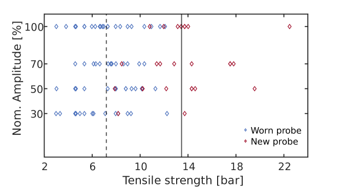
Figure 7: Scatter plot of the value of the water tensile strength as a function of the nominal amplitude set on the ultrasound device. The horizontal black line represents the average value of tensile strength for the experiments done with the worn probe (blue markers), while the horizontal dashed line indicates the average value for the experiments done with the new probe (red markers).

The estimated value of tensile strength ($p_{R}$) versus the nominal amplitude setting of the ultrasound device is shown in Fig. 7. Among the experimental configurations with the worn ultrasound probe (Conf. 1, 2, 3, 4) the minimum and the maximum value of the tensile strengths are respectively $3.05\text{\,}\mathrm{b}\mathrm{a}\mathrm{r}$ (Conf. 3) and $12.25\text{\,}\mathrm{b}\mathrm{a}\mathrm{r}$ (Conf. 3). Instead, among the experimental configuration with the 3 mm new probe (Conf. 5, 6, 7), the minimum and the maximum value of tensile strength are $7.88\text{\,}\mathrm{b}\mathrm{a}\mathrm{r}$ (Conf. 5) and $22.48\text{\,}\mathrm{b}\mathrm{a}\mathrm{r}$ (Conf. 5). Overall, with the new probe, water is able to withstand higher tensile strength ($p_{R}=13.46$ bar, vertical black line in Fig. 7), while with the worn probe, it tends to form cavitation at lower tensile strength ($p_{R}=7.18$ bar, vertical dashed line in Fig. 7). This is likely because of micro-pores and the roughness on the surface of the worn probes that act to reduce the energy barrier required for cavitation onset (Brennen, 2013). This behavior was predictable since we are dealing with a heterogeneous nucleation phenomenon (Fig. 3) (Brennen, 2013). These results confirm that water can withstand tension stresses before changing phase. All the experiments have been carried out by taking the temperature of the liquid water at 24^∘ C. The dissolved oxygen (DO) of the liquid water was not altered with preliminary treatments. The experiments have been conducted with a level of DO saturation percentage oscillating between 64 % and 84 %. However, the values of the tensile strength computed have not shown any clear trend with the corresponding values of DO measured before the experimental run. The range of results, obtained in the seven experimental configurations, is represented by the cyan-colored bar in Fig. 1 and is in good agreement with similar measurements performed by other authors: Esche (1952); Blake (1949); Strasberg (1959).

3 Definition of a new Cavitation Number

The agreement of the results, with the experimental data (Fig. 1), suggests the validity of the method proposed. However, the previous results are based on a strong assumption: cavitation only depends on the near-field, and the reflection of the acoustic waves, on the wall of the container, can be neglected. The validity of this assumption can be verified by estimating the acoustic pressure amplitude of a wave reflecting on the wall of the container, along the axis of the probe. This can be done on the second configuration (Conf. 2) since it should provide the strongest pressure amplitude of the reflected wave. In this configuration, the distance between the tip of the ultrasound probe and the wall is 19.66 mm, and the acoustic reflective index between the water and the material of the wall (optical glass) is R = 0.94. Since the relative position, between the emitting surface and wall, is larger than several probe’s diameters; the acoustic pressure can be evaluated by using the far-field approximation (Sherman and Butler, 2007;2011;; Kinsler et al., 2000):

$$p(r,\theta,t)=\frac{i}{2}\rho ckv_{0}\frac{d^{2}}{R}\left[\frac{2J_{1}(kd\sin{\theta})}{kd\sin{\theta}}\right]e^{i(\omega t-kR)},$$ (7)

where $R$ and $\theta$ are respectively the radial and the polar coordinates of a spherical reference system with the origin on the axis of the probe, on the emitting surface (Fig. 2). The azimuthal angle does not appear in Eq. 7 because of the axial symmetry (Fig. 2). The term $J_{1}$ in Eq. 7 is the First-Order Bessel Function (Sherman and Butler, 2007;2011;; Kinsler et al., 2000). Assuming a vibration amplitude of $20\text{\,}\mathrm{\SIUnitSymbolMicro}\mathrm{m}$ for the ultrasound probe in Conf. 2, the maximum acoustic pressure predicted in the near field is $6.69\text{\,}\mathrm{b}\mathrm{a}\mathrm{r}$, while the pressure amplitude of the wave reflected on the container’s wall, along the axis of the probe, is estimated to be $0.23\text{\,}\mathrm{b}\mathrm{a}\mathrm{r}$ ($1/R$ trend with the radial distance (Eq. 7)). This clearly demonstrates that the influence of the reflected acoustic wave can be neglected in the estimation of the pressure threshold for acoustic cavitation, as long as the wall of the container is placed at a sufficiently far distance from the emitting surface (far-field). A direct validation, of the analytical model (Eq. 4), adopted for the estimation of the acoustic pressure, can be obtained by comparison with the pressure measurements done with the hydrophone. In every experimental configuration, the hydrophone was placed in a certain point of the domain, in the far-field, where the acoustic pressure amplitude can be estimated, in polar coordinates, by using Eq. 7. The comparison between the analytical results and the hydrophone data is visible in Tab. 1. These are related to different nominal amplitudes and instants of time for Conf. 3.

$A_{nom}$ [%] Time [ms] Hydrophone Voltage [V] Hydrophone Pressure [bar] $A$ [m] $p_{0}$ [bar] Relative Error [%] 30 3 0.11 0.027 7.73E-06 0.026 5.36 30 3.5 0.155 0.038 9.02E-06 0.030 21.65 30 4 0.3 0.075 1.59E-05 0.054 28.62 50 3 0.15 0.037 9.70E-06 0.033 12.88 50 3.5 0.215 0.053 1.03E-05 0.035 35.17 50 4 0.415 0.103 1.29E-05 0.044 58.02 100 3 0.16 0.040 9.70E-06 0.033 18.33 100 3.5 0.27 0.067 1.10E-05 0.037 45.15 100 4 0.365 0.091 1.23E-05 0.041 54.65

Table 1: Comparison between the acoustic pressure amplitude ($p_{0}$) estimated with the analytical model and the measurement done with the hydrophone (Hydrophone Pressure). The data are related to different nominal amplitude and time instants for Conf. 3.

The data shows a good agreement between the value of the acoustic pressure amplitude predicted by the model and those measured by using the hydrophone. Even the largest deviation (58.02 % in Tab.1) can be justified by taking into account all the non-idealities present in the experimental setup: the limited resolution used in the tracking procedure for the estimation of the vibration amplitude, the uncertainty related to the position of the hydrophone with the respect of the ultrasound probe, and the influence of the acoustic wave reflected on the walls of the container. The increase of the relative error, as time progresses, could be due to a larger acoustic pressure of the reflected waves since the vibration amplitude of the probe also increases with time.

Given the experimental results obtained by the proposed framework, it is possible to define a new cavitation number (Viciconte et al., KAUST Research Repository, 15-06-2023), based on the definition of tensile strength and the estimation of the acoustic pressure with the analytical model (Eq. 5) :

$$Ca=\frac{p_{R}(f,T)+\rho gh-(p_{atm}-p_{r})}{2\rho cA\omega\left|\sin(\frac{kd}{2})\right|},$$ (8)

where $\rho gh$ is the hydrostatic pressure, $p_{r}$ is the reference pressure, and $p_{atm}$ is the atmospheric pressure. The tensile strength of the liquid medium ($p_{R}(f,T)$) appears, at the numerator, as a cavitation threshold, replacing the vapor pressure traditionally used in the context of hydrodynamic cavitation. The formulation of the denominator in Eq. 8 is only valid when using a circular transducer where $kd\leq\pi$ (Kinsler et al., 2000; Sherman and Butler, 2007;2011;). In the case of a transducer with $kd>\pi$, the formulation of the cavitation number takes the form of:

$$Ca=\frac{p_{R}(f,T)+\rho gh-(p_{atm}-p_{r})}{2\rho cA\omega}.$$ (9)

Starting from the theoretical arguments discussed and the experimental results obtained, it clearly arises that $p_{R}$, expressed in a general form, is a function of the frequency of the acoustic wave ($f$) and the temperature of the liquid medium ($T$). This dependency has not been directly investigated in the present work, since all the experiments have been run at fixed frequency and temperature of the liquid. We can generalize the equation further given that Eq. 8 and Eq. 9 are related to a plane circular piston. The cavitation number can be expressed more generally as:

$$Ca=\frac{p_{R}(f,T)+\rho gh-(p_{atm}-pr)}{C_{g}\rho cA_{0}\omega},$$ (10)

where the term $\rho cA_{0}\omega$ represents the acoustic pressure amplitude of a plane wave, solution of the one-dimensional acoustic wave equation (Kinsler et al., 2000; Lurton, 2010):

$$\frac{\partial^{2}p}{\partial t^{2}}=c^{2}\frac{\partial^{2}p}{\partial x^{2}}.$$ (11)

The term $C_{g}$ (Eq. 11) is a non-dimensional coefficient which is a function of the transducer (piston) geometry (for a circular piston $C_{g}=2\left|\sin\left[\frac{kd}{2}\right]\right|$). $C_{g}$ acts as a corrective factor, to make the denominator equal to the maximum acoustic pressure amplitude generated by a particular geometry. Thus, assuming to have a defined value of the tensile strength of the liquid medium, for a given temperature and frequency, when the maximum acoustic pressure amplitude (denominator) is smaller than the cavitation threshold (numerator), cavitation does not occur ($Ca>1$). On the contrary, if the acoustic pressure is larger than the numerator, cavitation occurs ($Ca<1$). It is important to clarify that the above definition (Eq. 10) is based on the assumption that cavitation happens in the near field and does not depend on the reflection of the acoustic waves on the boundaries of the domain.

4 Acoustic analogy to describe impulsive cavitation

The same approach proposed can be applied to study phenomena where cavitation is caused by an impulsive motion. We used a set of mallet-tube experiments, proposed by Pan et al. (2017a), to demonstrate the validity of the acoustic analogy for impulsive phenomena. Pan et al. (2017a) investigated the cavitation activity that occurs when a liquid-filled bottle is struck, from the top, by a mallet. Under the action of the impulsive force given by the mallet, the rapid acceleration of the bottle creates a rarefaction region in the liquid medium. This induces the formation and collapse of tiny bubbles at the bottom of the bottle (Pan et al., 2017a). The classical velocity-based cavitation number used to describe hydrodynamic cavitation (Brennen, 1994), is not able to represent cavitation in flows that undergoes an impulsive acceleration. For this reason, (Pan et al., 2017a) introduced Eq. 2.

The experimental data, analyzed in this section, are related to an experimental campaign done at the Utah State University and Brigham Young University (USU/BYU) (Daily, 2013; Daily et al., 2014; Pan et al., 2017a). For the experimental setup, the USU/BYU group used cylindrical transparent tubes, having an inner diameter ($D$) of $55\text{\,}\mathrm{mm}$. The tube was partially filled with distilled water and the internal reference pressure ($p_{r}$) was kept, through a pressure tap, to a value of $86.9\text{\,}\mathrm{k}\mathrm{P}\mathrm{a}$. The water properties considered by the authors can be found in (Pan et al., 2017a). The height of the liquid (h), within the tube, was varied in a range from $12.5\text{\,}\mathrm{mm}$ to $74.5\text{\,}\mathrm{mm}$. To investigate the influence of the tube material on cavitation, the authors tested three different materials: acrylic, polyethylene terephthalate, and polypropylene (Pan et al., 2017a).

The tube was accelerated by striking the top with a rubber mallet. For every experiment, the authors monitored the presence of cavitation bubbles, using a high-speed camera, and the acceleration of the tube over time, by placing an accelerometer on the tube bottom. The sampling interval of the accelerometer was $0.2\text{\,}\mathrm{ms}$. Additional details on the experimental setup used by the USU/BYU group can be found in Pan et al. (2017a). Pan et al. (2017a) just considered the maximum acceleration ($a_{max}$) measured by the hydrophone. However, to reinterpret the phenomenon, through an acoustic analogy, we must take into account the entire acceleration curve over time. By doing this, the acceleration function can be expressed as a summation of sine and cosine, and the characteristic frequencies, associated with the impulsive motion of the tube, can be extracted.

For every observation, the global acceleration data set was "cleaned" by considering just a temporal window of $1.8\text{\,}\mathrm{ms}$ in a neighborhood of the main acceleration impulse (Fig. 8). This is equivalent to taking just ten experimental data (red dots in Fig. 8), but it is enough to represent the relevant acceleration impulse induced by the mallet impact on the tube. The acceleration values (Fig. 8) are positive since the coordinate of the reference system of the accelerometer coincides with the axis of the tube and faces towards the outside.

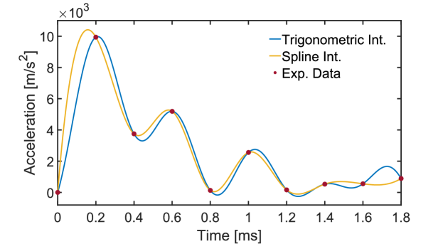
Figure 8: Experimental data, spline and trigonometric interpolation of the acceleration of the cavitation tube.

Taking into account the characteristic frequencies, associated with the impulsive acceleration of the tube, the data can be interpolated by a summation of trigonometric functions (Sauer, 2012). The acceleration is therefore defined as:

$$\begin{split}a(t)&=\frac{1}{\sqrt{n}}[\Re(y_{1})+\cos(\pi mtS_{f})\Re(y_{n/2+1})]+\\ &+\frac{2}{\sqrt{n}}\sum_{j=1}^{\frac{m}{2}-1}[\cos(2\pi jtS_{f})\Re(y_{j+1})-\sin(2\pi jtS_{f})\Im(y_{j+1})],\end{split}$$ (12)

where $j$ is the summation index, $n$ is the number of data points, $m$ is the order of the trigonometric function, $y_{j}$ is the j-th value of the DFT, and $t$ is the time variable. $\Re(y_{j})$ represents the real part of the j-th DFT value and $\Im(y_{j})$ represents the imaginary part. The trigonometric interpolation of the discrete data is obtained for $m=n$. $S_{f}$ is a scale factor which is a function of the sampling interval of the data, $\Delta t_{d}$ (equal to 0.2 ms in the current case), through the following relation:

$$S_{f}=\frac{0.1}{\Delta t_{d}}.$$ (13)

The blue curve in Fig. 8 represents the trigonometric interpolation of the experimental data (red dots in Fig. 8). The interpolation provided by Eq. 12 (Sauer, 2012) is similar to the Cubic Spline Interpolation (Inc., 2022) (orange curve in Fig. 8), and it seems to give a good representation of the experimental data (Fig. 8).

It is important to specify that the maximum frequency, described by the trigonometric interpolation (Eq. 12), is $2.5\text{\,}\mathrm{k}\mathrm{H}\mathrm{z}$ ($(\pi mS_{f})/(2\pi)$), while the sampling frequency of the experimental measurement is $5\text{\,}\mathrm{k}\mathrm{H}\mathrm{z}$ ($1/(\Delta t_{d})$). This is at the limit of validity of the Nyquist–Shannon Sampling Theorem (Gruber, 2013). However, to avoid any misrepresentation of the acceleration it would be better to have a higher sampling frequency. The velocity function can be found by integrating Eq. 12 with respect to time and by setting the integration constant equal to zero. All the terms arise as sine or cosine functions, except one which is linear in time. Since the acceleration impulse of the tube lasts a short interval of time (1.8 ms), it is possible to approximate the linear term as a sine one (Taylor expansion (Pourahmadi, 1984)): $(1/\sqrt{n})\Re(y_{1})t=(1/\sqrt{n})\Re(y_{1})\sin(t)$. Therefore, the velocity function can be entirely expressed as a summation of sine and cosine terms (Fig. 9):

$$\begin{split}v(t)&=\frac{1}{\sqrt{n}}[\Re(y_{1})\sin t+\frac{\Re(y_{n/2+1})}{\pi mS_{f}}\sin(\pi mtS_{f})]+\\ &+\frac{2}{\sqrt{n}}\sum_{j=1}^{\frac{m}{2}-1}[\frac{\Re(y_{j+1})}{2\pi jS_{f}}\sin(2\pi jtS_{f})+\frac{\Im(y_{j+1})}{2\pi jS_{f}}\cos(2\pi jtS_{f})].\end{split}$$ (14)

A characteristic frequency can be associated with every term of the function. This will simplify the solution of the wave equation for the estimation of the acoustic pressure within the tube.

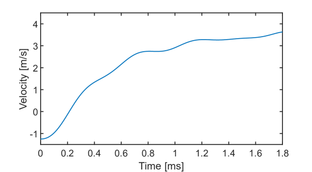
Figure 9: Trigonometric interpolation of the velocity function.

To describe this phenomenon, the mallet-tube problem can be modeled considering the plane circular transducer framework (Eq. 3) (Sherman and Butler, 2007;2011;; Kinsler et al., 2000). The acoustic analogy consists of considering the bottom of the tube as a vibrating surface of the transducer and the no-slip condition between the tube and the liquid medium. Under this analogy, the trigonometric interpolation of the velocity of the tube (Fig. 9) can be used as a boundary condition for the solution of the acoustic pressure (Eq. 5), derived from the Rayleigh’s integral (Rayleigh, 1896). The solution can be found separately for every trigonometric term of the velocity function (Eq. 14) and the global solution can be found by applying the Superposition Principle.

Since the maximum characteristic frequency, that describes the velocity function (Eq. 14), is equal to $2.5\text{\,}\mathrm{k}\mathrm{H}\mathrm{z}$ ($kd=0.30$); the maximum pressure amplitude occurs at the center of the tube bottom. Therefore, the acoustic pressure can be derived by using Eq. 5 and by considering the velocity amplitude $v_{0}^{i}$ associated with every term of the trigonometric velocity function (Eq. 14). In a generic form, the acoustic pressure ($p(r=0,x=0,t)$) is a summation of every $i$-th contribution, coming from the velocity equation:

$$\begin{split}p(r=0,x=0,t)=\sum_{i=1}^{n}\left[2\rho cv_{0}^{i}\left|\sin\left(\frac{k_{i}d}{2}\right)\right|\sin(\omega_{i}t+\phi_{i})\right].\end{split}$$ (15)

The acoustic pressure at the center of the tube’s bottom is shown in Fig. 10 where the minimum value correlates to cavitation ($p_{min}=-2.10$ bar). The negative value means that the liquid locally experiences a tensile deformation. The minimum value of the acoustic pressure was computed for all the experiments carried out by the USU/BYU group (Pan et al., 2017a; Daily et al., 2014; Daily, 2013). The tensile stress ($p_{T}$) is considered here instead of the acoustic pressure. Thus, the tensile stress can be computed by considering the presence of the hydrostatic contribution ($p_{hyd}=\rho gh$) and the reference pressure ($p_{r}$):

$$\begin{split}p_{T}=\lvert p_{min}+\rho gh-(p_{atm}-pr)\rvert.\end{split}$$ (16)

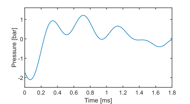
Figure 10: Acoustic pressure at the center of the bottom of the tube.

It is important to note that, in the above definition, the tensile stress is relative to the standard atmospheric pressure, following the convention used by Urick (1983) for the experimental chart in Fig. 1. Since the USU/BYU group monitored the cavitation inception (Pan et al., 2017a; Daily et al., 2014; Daily, 2013), for every experimental observation, it is possible to know whether the maximum acoustic tensile stress was able to generate or not cavitation at the bottom of the tube. This is synthesized in the scatter plot in Fig. 11, where the maximum tensile stress is plotted against the weighted average frequency of the pressure wave produced by the impulsive motion of the mallet. The open markers denote the presence of cavitation in the experimental observation, while the filled markers indicate the absence of cavitation activity. The makers in Fig. 11 are related to experiments carried out with three different tube materials: Acrylic, Polyethylene Terephthalate, and Polypropylene. The data, related to the acrylic and the polyethylene tubes, allow us to define a range around the presumed value of the tensile strength. Indeed, for these cases, the minimum value of the tensile stress able to generate cavitation is $0.97\text{\,}\mathrm{b}\mathrm{a}\mathrm{r}$, while the maximum value of the tensile stress not able to induce cavitation is $0.95\text{\,}\mathrm{b}\mathrm{a}\mathrm{r}$. These two values define a narrow range (black horizontal line in Fig. 11) in which the tensile strength should be contained.

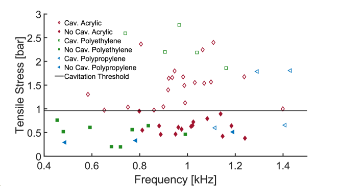
Figure 11: Scatter plot of derived from the application of the acoustic analogy on the mallet-tube experimental data, collected by the USU/BYU group (Daily, 2013; Daily et al., 2014; Pan et al., 2017a).

Regarding the experiments done with the tube made of polypropylene (Fig. 11), cavitation activity is observed for tensile stresses lower than $0.95\text{\,}\mathrm{b}\mathrm{a}\mathrm{r}$. This deviation, with respect to the cases with acrylic and polyethylene, could be due to the stiffness of the material. Indeed, polypropylene has a lower stiffness (Young modulus equal to $1.7\text{\,}\mathrm{G}\mathrm{P}\mathrm{a}$ (Pan et al., 2017b)). In this case, the assumption, that the acceleration of the bottom of the mallet is uniform across the entire surface (plane transducer), could fail. This could make invalid the application of the Rayleigh model used to estimate the acoustic pressure.

The tensile strength value can be compared with the experimental chart (red marker in Fig. 1) after being associated with the frequency of the phenomenon. Since multiple frequencies characterize the impulsive motion of the mallet-tube system, the weighted average frequency can be considered. The value of tensile strength (from $0.95\text{\,}\mathrm{b}\mathrm{a}\mathrm{r}$ to $0.97\text{\,}\mathrm{b}\mathrm{a}\mathrm{r}$), associated with the range of characteristic frequency of the impulsive cavitation phenomenon (from $0.48\text{\,}\mathrm{k}\mathrm{H}\mathrm{z}$ to $1.43\text{\,}\mathrm{k}\mathrm{H}\mathrm{z}$, Fig. 11), is in good agreement with the value of $1\text{\,}\mathrm{a}\mathrm{t}\mathrm{m}$ reported, for the same range of frequency, by Esche (1952) (Fig. 1).

The cavitation number, introduced before in Eq. 8, is valid when a singular frequency characterizes the acoustic system. In the case of summation of $n$ trigonometric functions at different characteristic frequencies, the formulation of the cavitation number is slightly more complicated:

$$\begin{split}Ca=\frac{p_{R}(f_{av})+\rho gh-(p_{atm}-pr)}{\left|min\left(\sum_{i=1}^{n}\left[2\rho cv_{0}^{i}\left|\sin(\frac{k_{i}d}{2})\right|\sin(\omega_{i}t+\phi_{i})\right]\right)\right|},\end{split}$$ (17)

the $i$-th elements are related to every trigonometric term of the velocity functions that describe the vibrating surface. This formulation of the cavitation number (Eq. 17) is related to a case where $n$ trigonometric functions describe the boundary condition that has to be applied to close the acoustic problem.

5 Conclusions

We introduced a novel cavitation number derived from the observation that, in acoustic systems, the vapor pressure is not a suitable indicator of cavitation. This dimensionless number is based on the definition of the tensile strength of a liquid medium and on the acoustic pressure, derived by using Rayleigh’s analytical model. The characteristic frequency of the phenomenon appears as a scaling factor in the cavitation number both at the denominator, in the acoustic pressure term, and at the numerator as an independent variable of the cavitation threshold. The cavitation onset was defined by using a procedure based on high-speed imaging and the acoustic signal measured by a hydrophone. The outputs of the two techniques were agreement in defining the instant of time at which cavitation occurs. This methodology could be used in the future for studying and characterizing the cavitation onset for other types of acoustic phenomena. When the methodology was applied to a cavitation event, induced by the impulsive action of a mallet on a tube containing water, this acoustic analogy accurately described the phenomenon.

Methodology

For the generation of ultrasound waves, in the liquid domain, an Hielscher device UP400S was used. This device works at a fixed nominal frequency of $24\text{\,}\mathrm{k}\mathrm{H}\mathrm{z}$, and it can provide a maximum power of $400\text{\,}\mathrm{W}$. A variable vibration amplitude can be set as a percentage of the maximum one. Cylindrical probes made of titanium, having different diameters can be installed on the ultrasound device. For the current study, two different cylindrical probes, having diameters of $7\text{\,}\mathrm{m}\mathrm{m}$ and $3\text{\,}\mathrm{m}\mathrm{m}$, have been used. Furthermore, both worn and new probes were tested. An experimental setup, based on the backlighting technique and the high-speed imaging, was adopted to capture the cavitation inception during the vibration of the ultrasound probe (Landeau et al., 2014). A schematic illustration of the backlighting setup is visible in Fig. 2. A LED light source (Godox SL-200W II), emitting white lite non-coherently, was placed on the back side of a water container and aligned with the axis of the ultrasound probe, which is immersed in the liquid water. The scene was captured using a high-speed camera (Photron Nova S16) placed in front of the container, at the opposite side of the LED light source (Fig. 2). The camera was triggered using the signal coming from a hydrophone (Aquarian AS-1 Hydrophone, calibration factor: $40\text{\,}\mathrm{\SIUnitSymbolMicro}\mathrm{V}$/Pa) (Fig. 2), and passing through an oscilloscope. Seven different configurations have been tested during the experimental campaign. These configurations differ for type of water, geometry and material of the transparent container, immersion depth of the probe, and relative position between the probe and the hydrophone. In the first (Conf. 1) and second configuration (Conf. 2) a 3 mm cylindrical probe and a transparent container made of optical glass and having an optical path of 50 mm (Hellma) were used. The water level in the container was 39 mm for both the configurations. The experiments related to Conf. 1 were run using distilled water from a local vendor, together with an immersion depth of the probe of 16.4 mm, and a distance between the axis of the probe and the acoustic center of the hydrophone of 34.7 mm. For Conf. 2, the immersion depth was set to 19.5 mm, and the probe/hydrophone distance to 34.5 mm. In this configuration an extra pure water, deionized (Thermo Fisher), was used. In the third (Conf. 3) and fourth (Conf. 4) configurations, Milli-Q water was placed in an transparent acrylic container, having a transversal section of 200 mm$\times$200 mm. The water level in the container was kept at 80 mm. In Conf. 3, a 3 mm cylindrical probe was used and submerged 20 mm below the free surface of the water. The distance between the probe and the acoustic center of the hydrophone was 74.2 mm. In Conf. 4, a 7 mm probe has been used, together with an immersion depth of 20 mm. In this case, the distance between the probe axis and the hydrophone was set to 70.7 mm. In the last three experimental configurations, Conf. 5, 6, and 7; a container made of optical glass (Hellma, 50 mm optical path) was used, together with a 3 mm probe, submerged 20 mm below the free surface. The types of water used were: distilled water from a local vendor (Conf. 5), extra pure water, deionized (Thermo Fisher), and pure water demineralized (Thermo Fisher). In Conf. 3, a Leica zoom lens (12x) was adopted. This lens can guarantee a level of magnification of 12x, providing a resolution of $1.28\text{\,}\mathrm{\SIUnitSymbolMicro}\mathrm{m}$. In the other configurations, a Mitutoyo 10X objective lens was used. This lens can guarantee a resolution of $1.98\text{\,}\mathrm{\SIUnitSymbolMicro}\mathrm{m}$. Since the nominal frequency of the ultrasound device is 24 kHz, the scene was recorded using a frame rate of 200000 fps (200 kHz). At this frame rate, The Nova S16 camera can guarantee an image size of 128x224 pixels. The shutter speed of the camera was set to 1/500000 s.

References

- Brennen [2013] Christopher Earls Brennen. Cavitation and bubble dynamics. 2013. ISBN 9781107338760. doi:10.1017/CBO9781107338760.
- Guida et al. [2022] Paolo Guida, Gianmaria Viciconte, Alberto Ceschin, Elia Colleoni, Francisco E Hernández Pérez, Saumitra Saxena, Hong G Im, and William L Roberts. Numerical model of an ultrasonically induced cavitation reactor and application to heavy oil processing. Chemical Engineering Journal Advances, 12:100362, 2022.
- Sharma et al. [2003] JB Sharma, Ashok Kumar, Arunaz Kumar, M Malhotra, R Arora, S Prasad, and S Batra. Effect of lycopene on pre-eclampsia and intra-uterine growth retardation in primigravidas. International Journal of Gynecology & Obstetrics, 81(3):257–262, 2003.
- Flores et al. [2021] Erico MM Flores, Giancarlo Cravotto, Cezar A Bizzi, Daniel Santos, and Gabrielle D Iop. Ultrasound-assisted biomass valorization to industrial interesting products: state-of-the-art, perspectives and challenges. Ultrasonics Sonochemistry, 72:105455, 2021.
- Suslick et al. [1999] Kenneth S Suslick, Yuri Didenko, Ming M Fang, Taeghwan Hyeon, Kenneth J Kolbeck, William B McNamara III, Millan M Mdleleni, and Mike Wong. Acoustic cavitation and its chemical consequences. Philosophical Transactions of the Royal Society of London. Series A: Mathematical, Physical and Engineering Sciences, 357(1751):335–353, 1999.
- Kozmus et al. [2022] Gregor Kozmus, Jure Zevnik, Marko Hočevar, Matevž Dular, and Martin Petkovšek. Characterization of cavitation under ultrasonic horn tip–proposition of an acoustic cavitation parameter. Ultrasonics sonochemistry, 89:106159, 2022.
- Suslick and Flannigan [2008] Kenneth S. Suslick and David J. Flannigan. Inside a Collapsing Bubble: Sonoluminescence and the Conditions During Cavitation. Annual Review of Physical Chemistry, 59(1):659–683, 2008. ISSN 0066-426X. doi:10.1146/annurev.physchem.59.032607.093739.
- Suslick [1990] Kenneth S Suslick. Sonochemistry. science, 247(4949):1439–1445, 1990.
- Didenko et al. [1999] Yuri T Didenko, William B McNamara, and Kenneth S Suslick. Hot spot conditions during cavitation in water. Journal of the American Chemical Society, 121(24):5817–5818, 1999.
- Wagterveld et al. [2011] RM Wagterveld, L Boels, MJ Mayer, and GJ Witkamp. Visualization of acoustic cavitation effects on suspended calcite crystals. Ultrasonics sonochemistry, 18(1):216–225, 2011.
- Smirnov et al. [2022] IV Smirnov, NV Mikhailova, BA Yakupov, and GA Volkov. Analysis of dependences of threshold parameters for acoustic cavitation onset in a liquid on an ultrasonic frequency, hydrostatic pressure, and temperature. Technical Physics, 67(2):161–170, 2022.
- Brennen [2011] Christopher E Brennen. Hydrodynamics of pumps. Cambridge University Press, 2011.
- Arndt [1981] Roger EA Arndt. Cavitation in fluid machinery and hydraulic structures. Annual Review of Fluid Mechanics, 13(1):273–326, 1981.
- Pan et al. [2017a] Zhao Pan, Akihito Kiyama, Yoshiyuki Tagawa, David J. Daily, Scott L. Thomson, Randy Hurd, and Tadd T. Truscott. Cavitation onset caused by acceleration. Proceedings of the National Academy of Sciences of the United States of America, 114(32):8470–8474, 2017a. ISSN 10916490. doi:10.1073/pnas.1702502114.
- Fatjo [2016] G Garcia-Atance Fatjo. New dimensionless number to predict cavitation in accelerated fluid. International Journal of Computational Methods and Experimental Measurements, 4(4):484–492, 2016.
- Lurton [2010] Xavier Lurton. An introduction to underwater acoustics: principles and applications. Springer, Berlin, second edition, 2010. ISBN 3540784802;9783540784807;.
- Gyftopoulos and Beretta [2005] E. P. Gyftopoulos and Gian P. Beretta. Thermodynamics: foundations and applications. Dover Publications, Mineola, N.Y, 2005. ISBN 0486439321;9780486439327;.
- Woods [1959] Leslie Colin Woods. The foundations of classical thermodynamics. 1959.
- Moebs et al. [2016] William Moebs, Samuel J Ling, and Jeff Sanny. University Physics Volume 1. Rice University, 2016.
- Berthelot [1850] Marcellin Berthelot. Sur quelques phenomemes de dilation force de liquids. Ann, Chimie Phys., 30:232–237, 1850.
- Pelton et al. [2013] Matthew Pelton, Debadi Chakraborty, Edward Malachosky, Philippe Guyot-Sionnest, and John E. Sader. Viscoelastic flows in simple liquids generated by vibrating nanostructures. Physical Review Letters, 111(24):1–5, 2013. ISSN 00319007. doi:10.1103/PhysRevLett.111.244502.
- Noirez and Baroni [2012] Laurence Noirez and Patrick Baroni. Identification of a low-frequency elastic behaviour in liquid water. Journal of Physics: Condensed Matter, 24(37):372101, 2012.
- Urick [1983] Robert J. Urick. Principles of underwater sound. McGraw-Hill, New York, third edition, 1983. ISBN 0932146627;0070660875;9780070660878;9780932146625;.
- Esche [1952] Rolf Esche. Untersuchung der schwingungskavitation in flüssigkeiten. Acta Acustica united with Acustica, 2(6):208–218, 1952.
- Strasberg [1959] M Strasberg. Onset of ultrasonic cavitation in tap water. The Journal of the Acoustical Society of America, 31(2):163–176, 1959.
- Blake [1949] F Gilman Blake. The onset of cavitation in liquids. Tech. Memo., (12), 1949.
- Dixon [1909] HENRY H Dixon. Note on the tensile strength of water, sci. In Proc. Roy. Dublin Soc, volume 12, pages 60–65, 1909.
- Caupin et al. [2012] Frédéric Caupin, Arnaud Arvengas, Kristina Davitt, Mouna El Mekki Azouzi, Kirill I Shmulovich, Claire Ramboz, David A Sessoms, and Abraham D Stroock. Exploring water and other liquids at negative pressure. Journal of Physics: Condensed Matter, 24(28):284110, 2012.
- Rayleigh [1896] John William Strutt Baron Rayleigh. The theory of sound, volume 2. Macmillan & Company, 1896.
- Viciconte et al. [KAUST Research Repository, 15-06-2023] Gianmaria Viciconte, Paolo Guida, Tadd Trevor Truscott, and William L Roberts. Unifying acoustic cavitation through the frequency. https://doi.org/10.25781/KAUST-T3980 (DOI:10.25781/KAUST-T3980), KAUST Research Repository, 15-06-2023.
- Inc. [2022] The MathWorks Inc. Matlab version: 9.13.0 (r2022b), 2022. URL https://www.mathworks.com.
- Sherman and Butler [2007;2011;] Charles H. Sherman and John L. Butler. Transducers and arrays for underwater sound. Springer, New York, 1. aufl. edition, 2007;2011;. ISBN 9780387329406;0387329404;9780387331393;0387331395;.
- Kinsler et al. [2000] Lawrence E Kinsler, Austin R Frey, Alan B Coppens, and James V Sanders. Fundamentals of acoustics. John wiley & sons, 2000.
- Pan et al. [2017b] Zhao Pan, Akihito Kiyama, Yoshiyuki Tagawa, David J Daily, Scott L Thomson, Randy Hurd, and Tadd T Truscott. Cavitation onset caused by acceleration. Proceedings of the National Academy of Sciences, 114(32):8470–8474, 2017b.
- Antkowiak et al. [2007] Arnaud Antkowiak, Nicolas Bremond, Stéphane Le Dizès, and Emmanuel Villermaux. Short-term dynamics of a density interface following an impact. Journal of Fluid Mechanics, 577:241–250, 2007.
- Brennen [1994] Christopher E Brennen. Radial and rotordynamic forces. Hydrodynamics of pumps. Oxford University Press and Concepts NREC, White River Junction, VT, 1994.
- Daily [2013] David Jesse Daily. Fluid-structure interactions with flexible and rigid bodies. Brigham Young University, 2013.
- Daily et al. [2014] Jesse Daily, Jonathon Pendlebury, Ken Langley, Randy Hurd, Scott Thomson, and Tadd Truscott. Catastrophic cracking courtesy of quiescent cavitation. Physics of Fluids, 26(9):091107, 2014.
- Sauer [2012] Timothy Sauer. Numerical analysis. 2nd ed., Boston: Pearson, 2012.
- Gruber [2013] Markus Gruber. Proofs of the nyquist-shannon sampling theorem. 2013.
- Pourahmadi [1984] Mohsen Pourahmadi. Taylor expansion of and some applications. The American Mathematical Monthly, 91(5):303–307, 1984.
- Landeau et al. [2014] Maylis Landeau, Renaud Deguen, and Peter Olson. Experiments on the fragmentation of a buoyant liquid volume in another liquid. Journal of fluid mechanics, 749:478–518, 2014.