Hierarchical Matrix Factorization for Interpretable Collaborative Filtering

Abstract

Matrix factorization (MF) is a simple collaborative filtering technique that achieves superior recommendation accuracy by decomposing the user-item rating matrix into user and item latent matrices. This approach relies on learning from user-item interactions, which may not effectively capture the underlying shared dependencies between users or items. Therefore, there is scope to explicitly capture shared dependencies to further improve recommendation accuracy and the interpretability of learning results by summarizing user-item interactions. Based on these insights, we propose “Hierarchical Matrix Factorization” (HMF), which incorporates clustering concepts to capture the hierarchy, where leaf nodes and other nodes correspond to users/items and clusters, respectively. Central to our approach, called hierarchical embeddings, is the additional decomposition of the user and item latent matrices (embeddings) into probabilistic connection matrices, which link the hierarchy, and a root cluster latent matrix. Thus, each node is represented by the weighted average of the embeddings of its parent clusters. The embeddings are differentiable, allowing simultaneous learning of interactions and clustering using a single gradient descent method. Furthermore, the obtained cluster-specific interactions naturally summarize user-item interactions and provide interpretability. Experimental results on rating and ranking predictions demonstrated the competitiveness of HMF over vanilla and hierarchical MF methods, especially its robustness in sparse interactions. Additionally, it was confirmed that the clustering integration of HMF has the potential for faster learning convergence and mitigation of overfitting compared to MF, and also provides interpretability through a cluster-centered case study.

1 Introduction

Matrix factorization (MF) [1] is a successful model-based approach for personalized recommender systems. The main idea is to decompose the matrix representing the observed interactions between users and items into two types of matrices: user-latent and item-latent matrices. The interaction between a user and item is then predicted by computing the inner product of the obtained user and item latent vectors. A common explanation is that each dimension in the user latent vector corresponds to the user’s preference, and each dimension in the item latent vector corresponds to the item’s characteristics. Recognized for its simplicity and power, MF is used in a variety of applications and has been applied to a wide range of deep-learning-based methods to improve accuracy [2, 3].

However, because the embeddings that exist for each user or item are learned independently for each interaction, how each embedding is learned can be a closed box. Given that each latent factor represents some preference or characteristic, it should be characterized based on supervised data; however, this is unrealistic. Instead, it is possible to focus on the cluster structure of objects that are potentially present in the data, such as the similarity between one item (user) and another. Therefore, by challenging the MF and clustering in a single model, it may be possible to improve the interpretability of MF through proximity between objects in the latent space, even if the embedding itself is not interpretable.

Several studies have been proposed that attempted to integrate the concept of clustering into MF, including methods for rating predictions [4, 5, 6] and ranking predictions [7]. These explicitly captured the user and item similarities in a dataset during the MF process. However, these approaches are specific to a particular situations (e.g., non-negative MF) or tasks (e.g., explicit or implicit recommendations), and therefore the cluster detection mechanisms may not be immediately applicable to recently developed MF methods.

Based on the above insights, we propose a hierarchical matrix factorization (HMF) method that captures the hierarchical structure of users and items in a dataset and is more generalizable than existing hierarchical MF methods in that it can be optimized with only a gradient descent scheme. The underlying concept is to assume a hierarchical relationship between the user and the item sets, such that the objects and clusters are represented by parent clusters. Inspired by the motivation behind fuzzy clustering [8], each user and item embedding are expressed as a weighted average of the parent cluster embeddings in the hierarchy. Therefore, HMF does not use the object embeddings as parameters; instead, it learns only the embeddings of the top-level clusters in the hierarchy and the connection matrices, which show the relationship between the sibling clusters. Simple hierarchical embedding has the following advantages. (1) Owing to its simple formulation and because the user and item embeddings are differentiable, a gradient method such as stochastic gradient descent (SGD) can be applied to the entire model if the upper task is also differentiable. Therefore, the HMF scheme can not only be easily applied not only to vanilla MF, but also to extended recent methods. (2) Hierarchical structures that exist implicitly can be captured naturally by learning the connection matrices. In other words, by learning a rating matrix, the hierarchical relationship between the user and item objects is automatically extracted, and how the MF learned its embedding can be interpreted through clusters as shown in Figure 1. (3) Learning the (composite) embedding of each object around the cluster points leads to stable loss convergence, as shown by the experimental results.

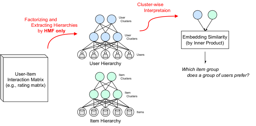
Figure 1: Graphical summary of our proposal framework. First, based on user-item interactions, the embeddings of users, items and their clusters as well as their hierarchy are extracted. Finally, the cluster embeddings are used for cluster-wise interpretation.

To confirm the effectiveness of the proposed method, two experiments were conducted: rating and ranking prediction. First, using the root mean squared error (RMSE) for rating prediction and the HitRatio and mean reciprocal rank (MRR) for ranking prediction, the recommendation accuracy of HMF was compared with that of the vanilla and hierarchical MF methods. In addition, to confirm the learning stability, we visualized the convergence of MF and HMF by sampling the hyperparameter settings that achieved the highest accuracy in the validation subset. Finally, as a case study, we demonstrated the predicted ratings between user and item clusters generated on a dataset and clarified how to interpret the trend of what HMF had learned.

In summary, our main contributions are as follows:

1. We propose an end-to-end model-based method HMF that simultaneously detects the user and item hierarchies through MF.

2. We introduce the proposed hierarchical embeddings, which are differentiable, into MF, allowing HMF to be optimized with a single gradient descent method.

3. We provide a summary of the cluster-level interactions from the obtained hierarchical embeddings, resulting in the interpretability of HMF.

The remainder of this paper is organized as follows. Section 2 reviews the concepts in MF and MF methods using clustering. Section 3 describes the components of hierarchical embeddings and the HMF learning scheme. Rating and ranking prediction experiments were performed, and the setup and results are summarized in Sections 4 and 5, respectively.

2 Related Work

2.1 MF and Its Extensions

MF is often explained in the context of an explicit feedback task, in which users assign a rating to certain items, such as five stars. Here, we assume $M$ users and $N$ items are available for the recommendation task. Subsequently, we can construct the rating matrix $\boldsymbol{X}\in\mathbb{R}^{M\times N}$ from the historical interactions, where each element $\boldsymbol{X}_{ij}$ denotes the rating of item $j$ provided by user $i$. The aim is to model each feedback interaction between user $i$ and item $j$ using the inner product of the $d$-dimensional user and item latent vectors $\boldsymbol{U}_{i},\boldsymbol{V}_{j}\in\mathbb{R}^{d}$:

$$\boldsymbol{X}_{ij}\approx\boldsymbol{U}_{i}^{T}\boldsymbol{V}_{j}$$ (1)

for all users and items in the task. In general, each “factor” in a user’s latent vector represents a preference of the user, such as liking a certain film genre. Similarly, each factor in an item’s latent vector represents its characteristics. Thus, computing the inner product allows us to express that a strong match between a user’s preferences and an item’s characteristics will result in a strong interaction (i.e., a high score) between the user and item.

Not all interactions between users and items can be observed in a real-world setting. For example, in e-commerce services, it is impossible for users to rate all products. The simplest way to deal with this problem is to treat the unobservables as zeros; however, because the resulting rating matrix is usually very sparse, this leads to an overfitted rating prediction. Therefore, the latent vectors are learned from the observed interactions using the following objective function:

$$\min_{\boldsymbol{U},\boldsymbol{V}}\sum_{(i,j)\in\boldsymbol{\Omega}}\left(\boldsymbol{X}_{ij}-\boldsymbol{U}_{i}^{T}\boldsymbol{V}_{j}\right)^{2}+\lambda_{\boldsymbol{\Theta}}||\boldsymbol{\Theta}||_{2}^{2}$$ (2)

where $\boldsymbol{\Omega}$ denotes the set of observed feedback, $\lambda_{\boldsymbol{\Theta}}$ is the regularization parameter, and $\boldsymbol{\Theta}$ represents the set of regularized parameters. SGD [1] and alternating least squares (ALS) [9] are primarily used as the optimizers. Then, in the context of the recommendation system, the resulting latent matrices are generally used to predict and recommend items that are likely to be highly valued by the user.

There are also many collaborative filtering settings for implicit feedback, such as “clicks,” “purchases,” “likes,” and “tagging.” It is inappropriate to use (2) because this is for implicit feedback that deals with the binary classification of whether an interaction has occurred and causes overfitting. Therefore, the objective functions, pointwise loss [10, 11, 12], pairwise loss [13], and softmax loss [14] have been proposed instead. In particular, Bayesian personalized ranking (BPR) [13] is a well-known method owing to its simplicity. The underlying idea is the probability that an observed interaction $(i,j)$ ranks higher than an unobserved interaction $(i,k)$. Therefore, the objective function is formulated as follows:

$$\min_{\boldsymbol{U},\boldsymbol{V}}-\sum_{\begin{subarray}{c}(i,j)\in\boldsymbol{\Omega},\\ (i,k)\notin\boldsymbol{\Omega}\end{subarray}}\ln\sigma(\boldsymbol{U}_{i}^{T}\boldsymbol{V}_{j}-\boldsymbol{U}_{i}^{T}\boldsymbol{V}_{k})+\lambda_{\boldsymbol{\Theta}}||\boldsymbol{\Theta}||_{2}^{2}$$ (3)

where $\sigma$ is a sigmoid function $\sigma(x)=(1+e^{-x})^{-1}$. The objective function is generally optimized using SGD and negative sampling (i.e., the sampling of unobserved interactions).

Although MF alone is a powerful tool, studies have attempted to further improve recommendation accuracy by introducing a neural network architecture [2, 3]. The common motivation of these studies is to overcome the linear model of MF and capture more complex user-item relationships by introducing nonlinearity and allowing representation learning. Deep matrix factorization [2] generates an interaction matrix based on user feedback, which is fed into a deep architecture to predict the interaction between the user and the item. Neural matrix factorization (NeuMF) [3] combines a generalization of MF with a neural architecture and a multilayer perceptron that captures the nonlinear relationship between users and items. As both are optimizable with SGD-based schemes, the MF architecture can be easily extended by applying SGD.

2.2 MF with Clustering

A pioneering approach is to use the hierarchical structure of objects obtained a priori to resolve sparsity in factorization [15]. Mashhoori et al. [16] modeled item vectors using a priori hierarchical relationships between items and successfully improved prediction accuracy compared to traditional MF. In practice, however, this hierarchical information is rarely available in a collaborative filtering setting, making it impractical; therefore, this setting is beyond the scope of this study. In addition, Hidden Group Matrix Factorization (HGMF) [17] detects groups of objects in the factorized matrix. However, the clustering and decomposition processes are independent and the classification information obtained during the decomposition may be overlooked.

Several methods have been proposed that simultaneously address clustering and factorization. In these, the clustering and factorization processes are interdependent. Capturing implicit hierarchical structures for recommender systems (known as IHSR) [18, 4] was the first approach to decomposes the latent matrices of users and items into latent matrices of the root nodes in the hierarchical structures and multiple affiliation matrices. By formulating this idea and applying a non-negative MF scheme, the strength of the relationship between levels can be obtained simultaneously. Hidden Hierarchical MF [5] also tackles hierarchical clustering and rating prediction simultaneously and consists of a bottom-up phase for learning the hidden hierarchical structure and a top-down phase for prediction. This method defines topics for groups of users and items and attempts to maximize the probability of generating a rating matrix and grouping the users and items using a quasi-Newton method. Learning tree-structured embeddings (known as eTREE) [6] include a new regularization term, which is the difference between the embedding of each child item and its parent item in a hierarchical structure. This method was optimized in the non-negative MF setup and used for rating prediction. Although it does not explicitly addressing clustering, the prototype-based MF method is also relevant. ProtoMF [7] defines a vector that measures the similarity between the embeddings of users and items and the embeddings of prototypes (similar to clusters). The inner product of these vectors models the implicit feedback.

Overall, these methods are limited to specific tasks (i.e., explicit or implicit feedback) and optimization techniques. It is questionable whether they can be directly applied to MF-based deep-learning methods, which have been increasingly developed in the context of representation learning in recent decades.

2.3 Interpretable Recommendation

It is essential to provide users and system vendors with the reasons for recommendations to improve non-accuracy metrics, including the transparency, persuasiveness, and reliability of the recommendations [19]. These techniques (not limited to recommendation systems) have been discussed in terms of interpretation and explanation, as defined in [20]:

• Interpretation – “the mapping of an abstract concept (e.g. a predicted class) into a domain that the human can make sense of.”

• Explanation – “the collection of features of the interpretable domain, that have contributed for a given example to produce a decision (e.g. classification or regression).”

As a well-known example, Xian et al. [21] proposed an attribute-aware recommendation that provides attributes corresponding to recommendations, and McAuley et al.  [22] attempted to explain latent dimensions in ratings by exploiting hidden topics in the review data.

Returning to the discussion of MF, it does not handle explicit features unless it takes the position of a hybrid approach that also uses user and item attribute information. Naturally, in collaborative filtering, reliable recommendations provided by MF focus on interpretability rather than explainability. A common approach to interpretability is to present a neighborhood-style reason, such as “your neighbor users rate this item highly,” which contains the idea of a memory-based approach [23, 24]. However, because the neighborhood-style reason depends on a per-user or per-item basis, as the number of users and items increases, it can be difficult to summarize how the model learns the entire dataset. ProtoMF [7], which assumes user and item prototypes, is capable of interpreting such prototype-item relationships to realize a summary of the interpretation of its model. Similarly, assuming hierarchical clusters of users and items, we aim to interpret them at a higher level of abstraction, such as “Which item group does a group of users prefer?”

3 Methodology

3.1 Representation of Users and Items

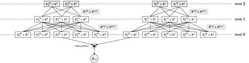
(a) 3-layer HMF

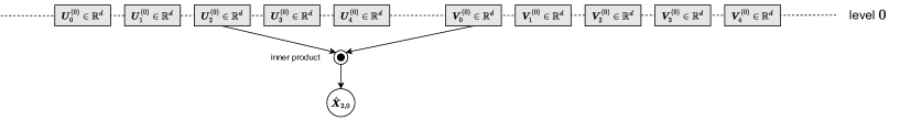
(b) MF

Figure 2: Example of differences between HMF and MF model architectures. Gray highlights indicate the model parameters trained on a dataset. MF has parameters (the latent variables) for each user and item, whereas HMF has latent variables in the root clusters and the connection parameters between levels.

We define a hierarchical structure with leaf nodes as users and items, respectively, and assume that nodes are characterized by their parent nodes (i.e., clusters). Specifically, a node embedding can be represented by the weighted average of the embeddings of its parent clusters within a latent space. A hierarchical structure with a depth of one is a simple clustering setup, whereas a deeper structure captures more complex structures and clusters of clusters. With respect to items, it is intuitive to assume a deep hierarchical structure, given that on an e-commerce site, items can be categorized into main categories (e.g., household goods), subcategories (e.g., detergents), and so on. Consequently, our focus is not on learning the individual user- and item-specific embeddings, but on learning the root cluster embeddings along with their connections (weights) to sibling nodes, as shown in Fig. 2 (a). In this study, we refer to the user and item embeddings generated by this scheme as hierarchical embeddings. This approach differs from the vanilla MF method, which focuses on learning embeddings that are directly linked to individual objects, as shown in Fig. 2 (b).

For simplicity, we first consider a user hierarchy of depth one (i.e., a non-hierarchical clustering setting). Let $m_{1}$ be the number of user clusters; then, we decompose the user latent matrix $\boldsymbol{U}^{(0)}\in\mathbb{R}^{M\times d}$ into the connection matrix $\tilde{\boldsymbol{U}}^{(1)}\in\mathbb{R}^{M\times m_{1}}$ from users to clusters and the $m_{1}$ root cluster latent matrix $\boldsymbol{U}^{(1)}\in\mathbb{R}^{m_{1}\times d}$:

$$\boldsymbol{U}^{(0)}=\tilde{\boldsymbol{U}}^{(1)}\boldsymbol{U}^{(1)}.$$ (4)

We use the constraint $\sum_{s}\tilde{\boldsymbol{U}}_{is}^{(1)}=1$ for each user $i$, such that the connection matrix represents the probability that users are associated with clusters. Consequently, each user’s embedding (i.e., each row of $\boldsymbol{U}^{(0)}$) is represented by a weighted average of the cluster embeddings. This is clearly different from IHSR [18, 4], which imposes that all elements in its matrices are non-negative real numbers.

In the hierarchical setting, more coarse clusters must be generated from the clusters. Here, we consider a user hierarchy of depth $p$; that is, we iteratively cluster users or the last generated user clusters $p$ times. Let the level-specific number of user clusters be $\{m_{1},m_{2},\dots,m_{p}\}$ and $m_{0}=M$. This means that there are $m_{0}$ users at level zero and $m_{l}$ user clusters at level $l$. Then, the user latent matrix $\boldsymbol{U}^{(0)}$ can be reformulated using recursive decomposition:

$$\boldsymbol{U}^{(0)} =\tilde{\boldsymbol{U}}^{(1)}\boldsymbol{U}^{(1)}$$ (5)

$$=\tilde{\boldsymbol{U}}^{(1)}\tilde{\boldsymbol{U}}^{(2)}\boldsymbol{U}^{(2)}$$ (6)

$$=\tilde{\boldsymbol{U}}^{(1)}\tilde{\boldsymbol{U}}^{(2)}\cdots\tilde{\boldsymbol{U}}^{(p)}\boldsymbol{U}^{(p)}$$ (7)

where $\tilde{\boldsymbol{U}}^{(l)}\in\mathbb{R}^{m_{l-1}\times m_{l}}$ represents the connection matrix from user clusters (or user objects) at level $(l-1)$ to user clusters at level $l$, such that $\sum_{s}\tilde{\boldsymbol{U}}_{is}^{(l)}=1,\forall{i}$, and $\boldsymbol{U}^{(l)}\in\mathbb{R}^{m_{l}\times d}$ represents the embeddings of user clusters at level $l$.

The item latent matrix can be formulated similarly. Considering an item hierarchy with depth $q$, let $\{n_{1},n_{2},\dots,n_{q}\}$ be the level-specific number of item clusters and $n_{0}=N$. The item latent matrix $\boldsymbol{V}^{(0)}\in\mathbb{R}^{N\times d}$ is expressed recursively as follows:

$$\boldsymbol{V}^{(0)} =\tilde{\boldsymbol{V}}^{(1)}\boldsymbol{V}^{(1)}$$ (8)

$$=\tilde{\boldsymbol{V}}^{(1)}\tilde{\boldsymbol{V}}^{(2)}\boldsymbol{V}^{(2)}$$ (9)

$$=\tilde{\boldsymbol{V}}^{(1)}\tilde{\boldsymbol{V}}^{(2)}\cdots\tilde{\boldsymbol{V}}^{(q)}\boldsymbol{V}^{(q)}$$ (10)

where $\tilde{\boldsymbol{V}}^{(l)}\in\mathbb{R}^{n_{l-1}\times n_{l}}$ represents the connection matrix from item clusters (or items when $l=1$) at level $l-1$ to item clusters at level $l$ and $\boldsymbol{V}^{(l)}\in\mathbb{R}^{n_{l}\times d}$ represents the embeddings of item clusters at level $l$. Similarly, the connection matrices $\tilde{\boldsymbol{V}}^{(l)}$ satisfy $\sum_{t}\tilde{\boldsymbol{V}}_{jt}^{(l)}=1,\forall{j}$.

Note that these hierarchical embeddings (i.e., (7) and (10)) are clearly differentiable with respect to their connection matrices and the latent factors of the top-level clusters. Thus, the embedding part of the MF, which is differentiable with respect to the latent factors, can be easily replaced by a hierarchical embedding, and SGD can be used for optimization without modification. In addition, the embedding layer can be easily changed to hierarchical embedding in MF-based deep-learning methods (although this was not addressed in this study).

3.2 Loss Function

3.2.1 Rating Prediction

As in the vanilla MF, the rating $\boldsymbol{X}_{ij}$ assigned by user $i$ to item $j$ can be modeled by the inner product of the embedding of user $i$ and item $j$. However, unlike MF, the object embeddings are not subject to learning. Consequently, using the mean squared error, the objective function can be defined as

$$\min_{\begin{subarray}{c}\tilde{\boldsymbol{U}}^{(1)},\cdots,\tilde{\boldsymbol{U}}^{(p)},\boldsymbol{U}^{(p)},\\ \tilde{\boldsymbol{V}}^{(1)},\cdots,\tilde{\boldsymbol{V}}^{(q)},\boldsymbol{V}^{(q)}\end{subarray}}\sum_{(i,j)\in\boldsymbol{\Omega}}\left(\boldsymbol{X}_{ij}-\boldsymbol{U}_{i}^{(0)T}\boldsymbol{V}_{j}^{(0)}\right)^{2}$$

$$+\lambda_{\boldsymbol{\Theta}}||\boldsymbol{\Theta}||_{2}^{2}$$ (11)

$$\mathrm{s.t.}\quad \sum_{s}\tilde{\boldsymbol{U}}_{is}^{(l)}=1,\forall{i},\forall{l}\in\{1,\dots,p\}$$

$$\sum_{t}\tilde{\boldsymbol{V}}_{jt}^{(l)}=1,\forall{j},\forall{l}\in\{1,\dots,q\}$$

where

$$\boldsymbol{U}^{(0)}=\tilde{\boldsymbol{U}}^{(1)}\tilde{\boldsymbol{U}}^{(2)}\cdots\tilde{\boldsymbol{U}}^{(p)}\boldsymbol{U}^{(p)}$$

$$\boldsymbol{V}^{(0)}=\tilde{\boldsymbol{V}}^{(1)}\tilde{\boldsymbol{V}}^{(2)}\cdots\tilde{\boldsymbol{V}}^{(q)}\boldsymbol{V}^{(q)}.$$

However, the constraint of the above objective function to normalize the connection matrix row-by-row does not allow the typical gradient-based optimizer to be applied without some effort. Therefore, instead of this constraint, we apply a row-wise softmax function to the connection matrices. Finally, the objective function of HMF for rating prediction is

$$\min_{\begin{subarray}{c}\tilde{\boldsymbol{U}}^{(1)},\cdots,\tilde{\boldsymbol{U}}^{(p)},\boldsymbol{U}^{(p)},\\ \tilde{\boldsymbol{V}}^{(1)},\cdots,\tilde{\boldsymbol{V}}^{(q)},\boldsymbol{V}^{(q)}\end{subarray}}\sum_{(i,j)\in\boldsymbol{\Omega}}\left(\boldsymbol{X}_{ij}-\boldsymbol{U}_{i}^{(0)T}\boldsymbol{V}_{j}^{(0)}\right)^{2}+\lambda_{\boldsymbol{\Theta}}||\boldsymbol{\Theta}||_{2}^{2}$$ (12)

where

$$\boldsymbol{U}^{(0)} =\tilde{\tilde{\boldsymbol{U}}}^{(1)}\tilde{\tilde{\boldsymbol{U}}}^{(2)}\cdots\tilde{\tilde{\boldsymbol{U}}}^{(p)}\boldsymbol{U}^{(p)}$$

$$\boldsymbol{V}^{(0)} =\tilde{\tilde{\boldsymbol{V}}}^{(1)}\tilde{\tilde{\boldsymbol{V}}}^{(2)}\cdots\tilde{\tilde{\boldsymbol{V}}}^{(q)}\boldsymbol{V}^{(q)}$$

$$\tilde{\tilde{\boldsymbol{U}}}^{(l)} =\mathrm{softmax}(\tilde{\boldsymbol{U}}^{(l)}),\forall{l}\in\{1,\dots,p\}$$

$$\tilde{\tilde{\boldsymbol{V}}}^{(l)} =\mathrm{softmax}(\tilde{\boldsymbol{V}}^{(l)}),\forall{l}\in\{1,\dots,q\}.$$

3.2.2 Ranking Prediction

HMF can be easily applied to ranking prediction algorithms that are optimized based on the gradient descent algorithm. Here, we consider BPR-HMF, which is an extension of BPR to the HMF scheme. The objective function is derived by replacing the MF terms in the BPR objective function (3), as follows:

$$\min_{\begin{subarray}{c}\tilde{\boldsymbol{U}}^{(1)},\cdots,\tilde{\boldsymbol{U}}^{(p)},\boldsymbol{U}^{(p)},\\ \tilde{\boldsymbol{V}}^{(1)},\cdots,\tilde{\boldsymbol{V}}^{(q)},\boldsymbol{V}^{(q)}\end{subarray}}-\sum_{\begin{subarray}{c}(i,j)\in\boldsymbol{\Omega},\\ (i,k)\notin\boldsymbol{\Omega}\end{subarray}}\log\sigma(\boldsymbol{U}_{i}^{(0)T} \boldsymbol{V}_{j}^{(0)}-\boldsymbol{U}_{i}^{(0)T}\boldsymbol{V}_{k}^{(0)})+\lambda_{\boldsymbol{\Theta}}||\boldsymbol{\Theta}||_{2}^{2}$$ (13)

where

$$\boldsymbol{U}^{(0)} =\tilde{\tilde{\boldsymbol{U}}}^{(1)}\tilde{\tilde{\boldsymbol{U}}}^{(2)}\cdots\tilde{\tilde{\boldsymbol{U}}}^{(p)}\boldsymbol{U}^{(p)}$$

$$\boldsymbol{V}^{(0)} =\tilde{\tilde{\boldsymbol{V}}}^{(1)}\tilde{\tilde{\boldsymbol{V}}}^{(2)}\cdots\tilde{\tilde{\boldsymbol{V}}}^{(q)}\boldsymbol{V}^{(q)}$$

$$\tilde{\tilde{\boldsymbol{U}}}^{(l)} =\mathrm{softmax}(\tilde{\boldsymbol{U}}^{(l)}),\forall{l}\in\{1,\dots,p\}$$

$$\tilde{\tilde{\boldsymbol{V}}}^{(l)} =\mathrm{softmax}(\tilde{\boldsymbol{V}}^{(l)}),\forall{l}\in\{1,\dots,q\}.$$

Because the replaced terms are differentiable, gradient descent methods such as SGD can be applied to BPR-HMF as well as to BPR.

4 Experimental Setup

This section describes the experimental settings used in this study, including the datasets, baselines for comparison, and evaluation metrics.

4.1 Datasets

Table 1: Dataset statistics after filtering.

	# of Users	# of Items	# of Interactions	Density
			(training / validation / test)
ML-100K	625	1,561	64,000 / 2,775 / 1,932	0.0704
ML-1M	4,463	3,594	640,133 / 33,344 / 68,816	0.0463
Ciao	1,786	9,004	23,081 / 709 / 211	0.0015
DIGINETICA	24,933	54,859	180,894 / 2,324 / 1,398	0.0004

For the evaluation, we conducted rating and ranking prediction tasks utilizing three datasets (ML-100K, ML-1M, Ciao) and one dataset (DIGINETICA) respectively.

• ML-100K [25] – Movie domain dataset. A total of 100,000 five-star ratings have been given to 1,682 movies by 943 users. All users have at least 20 ratings.

• ML-1M [25] – Movie domain dataset. 6,040 users have given a total of 1,000,209 five-star ratings to 3,952 movies. All users have at least 20 ratings.

• Ciao [26] – Product domain dataset. We only used the released parts of the dataset. A total of 36,065 five-star ratings were given by 2,248 users to 16,861 products.

• DIGINETICA – E-commerce domain dataset. This contains user sessions and product information from an e-commerce site. We only used item view data (train-item-views.csv) from January 1 to June 1 for this experiment. Some sessions were missing user IDs or had multiple user IDs. Therefore, the last user ID in each session was used as the user ID for that session, and sessions with no IDs were deleted. The session ID was then removed, and the view between user and item was treated as implicit feedback.

Each dataset was divided into three subsets: training, validation, and testing. Temporal global split [27] was used as the splitting strategy for evaluation in a realistic prediction task. For ML-100K, ML-1M, and Ciao, all the interactions were sorted by timestamp and split into training (80%) and testing (20%) subsets. Furthermore, the last 20% of the training subset was used for validation. Note that, unlike previous studies, users and items with a few ratings were not deleted. In DIGINETICA, interactions were divided by timestamp: January to March into the training subset, April into the validation subset, and May and June 1 into the testing subset. Users with less than five views in the training subset were removed from all subsets. None of the methods, including the baselines, considered cold-start users or items. Therefore, users and items that were not included in the training subset were removed from the validation and test evaluations. Table 1 lists the statistics of the dataset used after these splits and filters.

4.2 Baseline and Proposed Methods

Table 2: Hyperparameter settings for the models in this study.

Model	Hyperparameter	Range
All	Embedding size $d$	$20$
MF, HMF, BPR-MF, NeuMF, ProtoMF, BPR-HMF	Weight decay of AdamW	$10^{-2},10^{-3},10^{-4},10^{-5},0$
	Learning rate	$10^{-2},10^{-3},10^{-4}$
	Batch size	$1024$
MF, HMF	# of epoch	512
BPR-MF, NeuMF, ProtoMF, BPR-HMF	# of epoch	128
IHSR, HMF	# of user clusters	$200,400,600,800,1000$
	# of item clusters	$100,200,300,400,500$
ProtoMF, BPR-HMF	# of user clusters	$\lfloor 24933/512\rfloor,\lfloor 24933/128\rfloor,\lfloor 24933/32\rfloor$
	# of item clusters	$\lfloor 54859/512\rfloor,\lfloor 54859/128\rfloor,\lfloor 54859/32\rfloor$
IHSR	Regularization parameter $\lambda$	$0,10^{-4},10^{-3},10^{-2},10^{-1},1,10$
	Maximum # of iterations	$64$
NeuMF	Hidden layer sizes for MLP	$\{40,20,10\}$
eTREE	# of item clusters by levels	$\{10\},\{25,5\},\{50,10,3\}$
	Regularization parameter $\lambda,\mu$	$10^{-3},0.5,1,5,10,15,20$
	Regularization parameter $\eta$	1000
ProtoMF	Tuning parameter $\lambda_{1},\lambda_{2},\lambda_{3},\lambda_{4}$	$10^{-3},10^{-2},10^{-1},1,10$

For comparison, we used several vanilla and state-of-the-art hierarchical MF methods for rating and ranking predictions.

• MF [1] – A vanilla MF method for explicit feedback. The user-item relationship is captured by decomposing a rating matrix into user and an item latent matrices.

• IHSR [18, 4] – A hierarchical MF method for explicit feedback. This captures the hierarchical structure of users/items by recursively decomposing the non-negative user/item latent matrix into non-negative matrices.

• eTREE [6] – A hierarchical MF method for explicit feedback. This constructs only an item hierarchy, which minimizes the difference between the embeddings of a node and its parent clusters, represented in the loss function as a regularization term.

• HMF (Proposed) – A hierarchical MF method for explicit feedback. This captures the user/item hierarchical structure by recursively decomposing the user/item latent matrix into the user/item latent matrix of root clusters and connection matrices between hierarchy levels.

• BPR-MF [13] – An MF method for implicit feedback. The interaction matrix is decomposed into user and item latent matrices so that the probability that the observed interaction is higher than the unobserved interaction is maximized, which is modeled using the sigmoid function.

• NeuMF [3] – A neural collaborative filtering method for implicit feedback. This is a pioneering method that extends MF to a deep learning base by combining a generalization of MF with a neural architecture and a multilayer perceptron that captures the nonlinear relationship between users and items.

• ProtoMF [7] – A prototype-based MF method for implicit feedback. This defines a similarity vector between the user/item latent vector and the prototype latent vector, and models implicit feedback by the inner product of the user and item similarity vectors. This method can be viewed as a hierarchical MF with a depth of one.

• BPR-HMF (Proposed) – A hierarchical MF method for implicit feedback. This is a combination of BPR and the proposed hierarchical embeddings.

All methods had certain hyperparameters. The number of embedding dimensions for all methods was fixed at 20, and the other parameters were tuned in the validation set using a grid search. Table 2 lists the details of the grid search range setting for each method. For fairness, all the methods were compared with a depth one, except for eTREE, for which the hyperparameter settings are publicly available. For the gradient descent methods, AdamW [28] was used as the optimizer and weight decay was used instead of the model parameter regularization term.

4.3 Evaluation Metrics

For the rating prediction tasks, we used the RMSE, which is the standard for evaluating regression tasks.

$$\mathrm{RMSE}=\sqrt{\frac{1}{|\boldsymbol{\Omega}|}\sum_{(i,j)\in\boldsymbol{\Omega}}(\boldsymbol{X}_{ij}-\hat{\boldsymbol{X}}_{ij})^{2}}$$ (14)

where $\boldsymbol{\Omega}$ represents the set of observed interactions in a validation or test subset, and $\boldsymbol{X}_{ij}$ and $\hat{\boldsymbol{X}}_{ij}$ represents the true and predicted ratings given by user $i$ for item $j$ by a method, respectively.

To evaluate the ranking prediction task, we prepared 100 item candidates, of which one was a positive-interacting item and 99 were negative-interacting items. That is, for a given observed interaction (user $i$ views item $j$) in the validation or testing subset, we randomly sampled 99 items that had not been viewed by user $i$ (i.e., negative sampling). The 100 items were then ranked by a trained model and scored using HitRatio@$10$ and MRR@$10$. HitRatio@$10$ scores one if the positive sample is in the top 10 and zero otherwise. The scores are then averaged for all interactions. MRR@$10$ scores the reciprocal of the rank ($rank$) of the positive samples in the top 10, that is, $1/rank$. If the positive sample is not in the top 10, it is set to zero. Similarly, the scores are averaged for all interactions.

To reduce the experimental duration, the training was terminated if the learning results did not improve for five consecutive epochs (or iterations) on the validation set. We trained all the methods with five different seeds, and for each method, the hyperparameter set with the highest average results based on the RMSE and HitRatio of the validation subset was selected. The average of the five evaluations of the testing subset using the hyperparameters was then reported.

5 Results

5.1 Accuracy Comparison

Table 3: Evaluation results in rating and ranking prediction tasks

Method	ML-100K	ML-1M	Ciao	DIGINETICA
	RMSE $\pm$ std	RMSE $\pm$ std	RMSE $\pm$ std	HitRatio@10 $\pm$ std	MRR@10 $\pm$ std
MF	1.113 $\pm$ 0.013	0.913 $\pm$ 0.002	2.306 $\pm$ 0.017	-	-
IHSR	1.080 $\pm$ 0.002	0.951 $\pm$ 0.000	1.122 $\pm$ 0.001	-	-
eTREE	1.082 $\pm$ 0.006	0.922 $\pm$ 0.003	1.254 $\pm$ 0.045	-	-
HMF	1.066 $\pm$ 0.002	0.920 $\pm$ 0.003	0.939 $\pm$ 0.001	-	-
BPR-MF	-	-	-	0.314 $\pm$ 0.019	0.153 $\pm$ 0.013
NeuMF	-	-	-	0.307 $\pm$ 0.009	0.150 $\pm$ 0.005
ProtoMF	-	-	-	0.277 $\pm$ 0.027	0.122 $\pm$ 0.011
BPR-HMF	-	-	-	0.323 $\pm$ 0.004	0.126 $\pm$ 0.003

Table 3 presents the accuracy results of the proposed and the baseline methods for the testing subsets. The top four rows show a comparison of the methods specific to rating prediction, and the bottom four rows show a comparison of ranking prediction. On the small dataset ML-100K, the hierarchical methods IHSR, eTREE, and HMF showed superior accuracy, with the RMSE of HMF being 0.014 points lower than that of the second best, IHSR. For the relatively large dataset ML-1M, HMF had the best accuracy among the hierarchical methods, whereas vanilla MF had the best accuracy overall. This slight degradation may be due to the insufficient tuning of the hyperparameter set for ML-1M, which has a large number of users and items. Specifying larger user or item clusters may have allowed HMF to outperform or match vanilla MF. For Ciao, a sparse dataset compared to the others, HMF showed a dramatic improvement over MF, which did not converge well. This suggests that a strong assumption of representative points can facilitate solution searching and provide robustness for sparse datasets. For ranking prediction and DIGINETICA, the proposed BPR-HMF method was the best in terms of HitRatio, but not MRR. This is because HMF assumes groups of items, which may make it difficult to push the rank of a particular item higher within a group, even though it may be possible to push the rank of the group to the top.

5.2 Loss Convergence

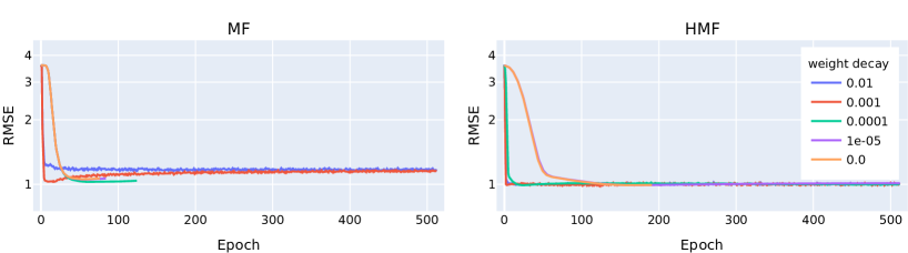
(a) ML-100K

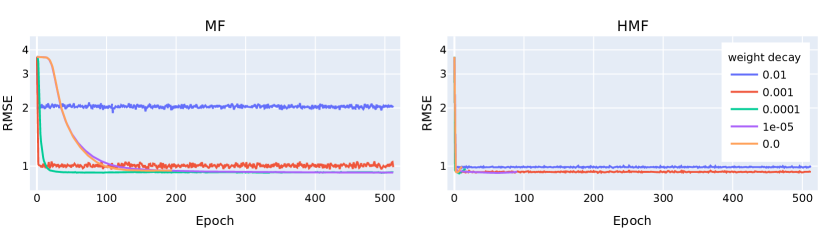
(b) ML-1M

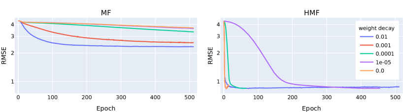
(c) Ciao

Figure 3: MF and HMF losses (shown in RMSE) per epoch on the validation subsets. The best hyperparameter setting was selected for each weight decay, showing the change in its loss. Note that if the validation loss increased for five consecutive epochs, the optimization was terminated.

To confirm the convergence of the HMF losses, which assumes clustering, we visualized the evolution of the losses for different hyperparameter settings. We selected the best hyperparameter setting in the validation subset for each weight decay (which corresponded to the strength of the parameter regularization) and tracked the changes in its RMSE. Fig. 3 shows the change in the RMSE of the validation subset per epoch for MF and HMF in the rating prediction tasks. In ML-100K, MF tended to slightly overfit, even with strong regularization; however, HMF tended to converge near to one regardless of regularization. This may be because of the clusters assumed by HMF, which may have had a regularization effect. In other words, because each user or item is represented by a weighted average of the clusters, it is less likely to be assigned an inappropriate position in the latent space. In ML-1M, MF required many epochs to converge, whereas HMF required approximately five epochs. Therefore, even when using the same SGD-based optimization method, that is, AdamW, the architecture of the model can cause convergence. For Ciao, which is considered difficult to learn owing to its high sparsity, MF did not converge well in any setting, whereas HMF converged to an RMSE of less than one in all setting. This suggests that hierarchical embedding in HMF not only speeds up convergence but also increases the probability of convergence.

5.3 Case Study

In HMF, all users, items, and their clusters are projected onto the same latent space, allowing the interpretation of similarities between clusters. In particular, identifying whether user representatives (clusters) think highly about item categories (clusters) has significant benefits for enhancing service quality. Herein, we present a case study of ML-1M for a movie service. Table 4 shows the inner products of the zeroth and first user clusters and all the item clusters, as well as the inner products of the 374th and 216th item clusters and all the user clusters. The inner product of the $i$-th user cluster and the $j$-th item cluster was computed as $\boldsymbol{U}_{i}^{(1)T}\boldsymbol{V}_{j}^{(1)}$. The user/item cluster size was calculated based on the weights of the connection matrix with a user/item of 1; that is, the size of the $j$-th user cluster ID is $\sum_{i}\tilde{\tilde{\boldsymbol{U}}}_{ij}^{(1)}$. In addition, item cluster titles characterized the item cluster and were the titles of items in the neighborhood (in terms of the inner product) of the item cluster in the latent space. Similarly, user cluster genders characterize the user cluster and were the genders of the users in the neighborhood (in terms of the inner product) of the user cluster.

Several observations can be made from Table 4. The zeroth user cluster has a high inner product with the item cluster containing horror movies and is favorable for horror movies like “Bride of the Monster” and “Braindead.” Therefore, these horror movies are the favorites for user cluster zero, and the cluster seems to capture similar movies, even though it only learns from explicit feedback. Additionally, it would be interesting to fix an item cluster to determine the group of users that prefer the item. It is possible that men preferred the 374th item cluster, whereas women had a negative opinion of it. By contrast, the opposite trend was observed for the 216th item cluster. Although this experiment confirmed the relationship between user and item clusters, it should be noted that the relationships between users and item clusters and between user clusters and items can also be confirmed.

Table 4: Case study of two user clusters and two item clusters on ML-1M. For each target user (item) cluster, the inner product with all item (user) clusters is computed and sorted in descending order.

(a) Target: 0th User Cluster
Item Cluster ID	Item Cluster Size	Item Cluster Titles	Inner Product
125	8.91	“Bride of the Monster”, “Godzilla (Gojira)”, “Rocky Horror Picture Show, The”	25.19
384	10.55	“Braindead”, “Bad Lieutenant”, “Bride of the Monster”	25.02
187	9.84	“Godzilla (Gojira)”, “Night of the Living Dead”, “Pee-wee’s Big Adventure”	24.80
$\vdots$	$\vdots$	$\vdots$	$\vdots$
309	7.50	“Patriot, The”, “Titanic”, “Pretty Woman”	-14.30
122	7.26	“Forrest Gump”, “Patriot, The”, “Shawshank Redemption, The”	-16.26
114	7.32	“Titanic”, “Lethal Weapon”, “Independence Day (ID4)”	-17.98
(b) Target: 1st User Cluster
Item Cluster ID	Item Cluster Size	Item Cluster Titles	Inner Product
288	7.58	“Fargo”, “Rushmore”, “American Beauty”	19.98
75	8.05	“Austin Powers: The Spy Who Shagged Me”, “Clockwork Orange, A”, “Austin Powers: International Man of Mystery”	18.66
349	7.87	“Fear and Loathing in Las Vegas”, “Pulp Fiction”, “Star Wars: Episode V - The Empire Strikes Back”	17.15
$\vdots$	$\vdots$	$\vdots$	$\vdots$
335	7.40	“Nil By Mouth”, “For Love of the Game”, “Girlfight”	-13.91
416	7.89	“For Love of the Game”, “Where the Heart Is”, “Bed of Roses”	-14.24
327	7.73	“Money Talks”, “Son of Flubber”, “Where the Heart Is”	-14.65
(c) Target: 374th Item Cluster
User Cluster ID	User Cluster Size	User Cluster Genders	Inner Product
35	5.24	M, M, M, M, M, M, M, M, M, M	23.07
232	5.19	M, M, M, M, M, M, M, M, M, M	22.53
404	7.28	M, M, F, M, M, M, M, M, F, F	20.68
$\vdots$	$\vdots$	$\vdots$	$\vdots$
86	6.43	M, M, F, F, F, M, F, M, M, M	-14.62
400	7.16	F, M, M, F, F, F, M, M, F, F	-15.24
624	7.85	F, M, M, F, M, M, M, M, M, M	-15.46
(d) Target: 216th Item Cluster
User Cluster ID	User Cluster Size	User Cluster Genders	Inner Product
156	8.35	F, M, F, F, M, F, M, M, F, M	30.95
61	6.26	F, F, F, M, M, F, F, M, M, F	29.17
200	6.62	F, F, F, F, M, M, F, M, F, F	27.89
$\vdots$	$\vdots$	$\vdots$	$\vdots$
94	9.28	M, M, M, M, M, M, M, M, M, M	-20.89
764	7.54	M, F, M, M, M, M, M, M, M, M	-23.41
347	5.91	M, M, M, M, M, M, M, M, M, M	-23.45

6 Conclusion

In this paper, we proposed HMF, which captures the hierarchical relationships between users and items in interpretable recommender systems. It is assumed that the embedding vector of the user/item or cluster is the weighted average of the embedding vectors of the parent clusters in the hierarchical structure. Under this assumption, the latent matrices of users and items are decomposed into an embedding matrix of the root clusters and connection matrices connecting the hierarchies, which are then incorporated into a vanilla MF. This simple devisal allowed us to tackle both MF and clustering with a single gradient method, and also facilitated the possibility of using it for recently developed MF methods based on the gradient method. Using real datasets, the proposed methods were evaluated in terms of recommendation accuracy, learning stability, and interpretability. Our methods equaled or outperformed existing hierarchical and vanilla MF methods, demonstrating competitiveness and robustness in particularly sparse interactions. Compared with MF, HMF showed convergence of the RMSE on the validation subset at an earlier epoch. In addition, the tendency to improve overfitting, even in later stages of training, suggests that clustering may play a role in regularization. By characterizing user and item clusters, we presented relationships between the clusters and provided an example of how we can interpret how HMF learns user and item interactions.

Nevertheless, this study has a few limitations. For example, allowing for soft clustering makes our interpretation more difficult, as similar item sets can belong to multiple item clusters, as listed in Table 4. This could be addressed by introducing a softmax function with temperature [29] to bias the degree of affiliation to a user/item and its clusters, i.e., be closer to a hard clustering setting. Second, although HMF supports hierarchical clustering, it does not sufficiently validate clustering settings deeper than a depth of two. A comprehensive evaluation of the appropriate depth and number of clusters in HMF is required in our future work.

Acknowledgments

This work was supported by JSPS KAKENHI Grant Numbers JP21H03553, JP22H03698.

Declarations

Funding This work was supported by JSPS KAKENHI, Grant Numbers JP21H03553 and JP22H03698.

Competing interests The authors have no relevant financial or non-financial interests to disclose.

Author contributions All the authors contributed to the conception and design of the study. Kai Sugahara invented the proposed algorithm and performed experiments and analyses. Kazushi Okamoto supervised development, experimentation, and analysis. The first draft of the manuscript was written by Kai Sugahara, and all the authors commented on the previous versions of the manuscript. All authors have read and approved the final manuscript.

Data availability All data generated or analyzed during this study are available from the corresponding author upon reasonable request.

References

- \bibcommenthead
- Koren et al. [2009] Koren, Y., Bell, R., Volinsky, C.: Matrix factorization techniques for recommender systems. Computer 42(8), 30–37 (2009) https://doi.org/10.1109/MC.2009.263
- Xue et al. [2017] Xue, H.-J., Dai, X.-Y., Zhang, J., Huang, S., Chen, J.: Deep matrix factorization models for recommender systems. In: Proceedings of the 26th International Joint Conference on Artificial Intelligence, pp. 3203–280933209 (2017)
- He et al. [2017] He, X., Liao, L., Zhang, H., Nie, L., Hu, X., Chua, T.-S.: Neural collaborative filtering. In: Proceedings of the 26th International Conference on World Wide Web, pp. 173–28093182 (2017). https://doi.org/10.1145/3038912.3052569
- Wang et al. [2018] Wang, S., Tang, J., Wang, Y., Liu, H.: Exploring hierarchical structures for recommender systems. IEEE Transactions on Knowledge and Data Engineering 30(6), 1022–1035 (2018) https://doi.org/10.1109/TKDE.2018.2789443
- Li et al. [2019] Li, H., Liu, Y., Qian, Y., Mamoulis, N., Tu, W., Cheung, D.W.: Hhmf: hidden hierarchical matrix factorization for recommender systems. Data Mining and Knowledge Discovery 33, 1548–280931582 (2019) https://doi.org/10.1007/s10618-019-00632-4
- Almutairi et al. [2021] Almutairi, F.M., Wang, Y., Wang, D., Zhao, E., Sidiropoulos, N.D.: etree: Learning tree-structured embeddings. Proceedings of the AAAI Conference on Artificial Intelligence 35(8), 6609–6617 (2021) https://doi.org/10.1609/aaai.v35i8.16818
- Melchiorre et al. [2022] Melchiorre, A.B., Rekabsaz, N., Ganhör, C., Schedl, M.: Protomf: Prototype-based matrix factorization for effective and explainable recommendations. In: Proceedings of the 16th ACM Conference on Recommender Systems, pp. 246–28093256 (2022). https://doi.org/10.1145/3523227.3546756
- Oh et al. [2001] Oh, C.-H., Honda, K., Ichihashi, H.: Fuzzy clustering for categorical multivariate data. In: Proceedings Joint 9th IFSA World Congress and 20th NAFIPS International Conference, vol. 4, pp. 2154–21594 (2001). https://doi.org/10.1109/NAFIPS.2001.944403
- Pan et al. [2008] Pan, R., Zhou, Y., Cao, B., Liu, N.N., Lukose, R., Scholz, M., Yang, Q.: One-class collaborative filtering. In: 2008 Eighth IEEE International Conference on Data Mining, pp. 502–511 (2008). https://doi.org/10.1109/ICDM.2008.16
- Hu et al. [2008] Hu, Y., Koren, Y., Volinsky, C.: Collaborative filtering for implicit feedback datasets. In: 2008 Eighth IEEE International Conference on Data Mining, pp. 263–272 (2008). https://doi.org/10.1109/ICDM.2008.22
- Ning and Karypis [2011] Ning, X., Karypis, G.: Slim: Sparse linear methods for top-n recommender systems. In: 2011 IEEE 11th International Conference on Data Mining, pp. 497–506 (2011). https://doi.org/10.1109/ICDM.2011.134
- Bayer et al. [2017] Bayer, I., He, X., Kanagal, B., Rendle, S.: A generic coordinate descent framework for learning from implicit feedback. In: Proceedings of the 26th International Conference on World Wide Web, pp. 1341–280931350 (2017). https://doi.org/10.1145/3038912.3052694
- Rendle et al. [2009] Rendle, S., Freudenthaler, C., Gantner, Z., Schmidt-Thieme, L.: Bpr: Bayesian personalized ranking from implicit feedback. In: Proceedings of the Twenty-Fifth Conference on Uncertainty in Artificial Intelligence, pp. 452–28093461 (2009)
- Rendle [2022] Rendle, S.: In: Ricci, F., Rokach, L., Shapira, B. (eds.) Item Recommendation from Implicit Feedback, pp. 143–171 (2022). https://doi.org/10.1007/978-1-0716-2197-4_4
- Menon et al. [2011] Menon, A.K., Chitrapura, K.-P., Garg, S., Agarwal, D., Kota, N.: Response prediction using collaborative filtering with hierarchies and side-information. In: Proceedings of the 17th ACM SIGKDD International Conference on Knowledge Discovery and Data Mining, pp. 141–28093149 (2011). https://doi.org/10.1145/2020408.2020436
- Mashhoori and Hashemi [2012] Mashhoori, A., Hashemi, S.: Incorporating hierarchical information into the matrix factorization model for collaborative filtering. In: Intelligent Information and Database Systems, pp. 504–513. Springer, Berlin, Heidelberg (2012)
- Wang et al. [2014] Wang, X., Pan, W., Xu, C.: Hgmf: Hierarchical group matrix factorization for collaborative recommendation. In: Proceedings of the 23rd ACM International Conference on Conference on Information and Knowledge Management, pp. 769–28093778 (2014). https://doi.org/10.1145/2661829.2662021
- Wang et al. [2015] Wang, S., Tang, J., Wang, Y., Liu, H.: Exploring implicit hierarchical structures for recommender systems. In: Proceedings of the 24th International Conference on Artificial Intelligence, pp. 1813–280931819 (2015)
- Zhang and Chen [2020] Zhang, Y., Chen, X.: Explainable recommendation: A survey and new perspectives. Foundations and Trends® in Information Retrieval 14(1), 1–101 (2020) https://doi.org/10.1561/1500000066
- Montavon et al. [2018] Montavon, G., Samek, W., Müller, K.-R.: Methods for interpreting and understanding deep neural networks. Digital Signal Processing 73, 1–15 (2018) https://doi.org/10.1016/j.dsp.2017.10.011
- Xian et al. [2021] Xian, Y., Zhao, T., Li, J., Chan, J., Kan, A., Ma, J., Dong, X.L., Faloutsos, C., Karypis, G., Muthukrishnan, S., Zhang, Y.: Ex3: Explainable attribute-aware item-set recommendations. In: Proceedings of the 15th ACM Conference on Recommender Systems, pp. 484–28093494 (2021). https://doi.org/10.1145/3460231.3474240
- McAuley and Leskovec [2013] McAuley, J., Leskovec, J.: Hidden factors and hidden topics: Understanding rating dimensions with review text. In: Proceedings of the 7th ACM Conference on Recommender Systems, New York, NY, USA, pp. 165–28093172 (2013). https://doi.org/10.1145/2507157.2507163
- Abdollahi and Nasraoui [2017] Abdollahi, B., Nasraoui, O.: Using explainability for constrained matrix factorization. In: Proceedings of the Eleventh ACM Conference on Recommender Systems, pp. 79–2809383 (2017). https://doi.org/10.1145/3109859.3109913
- Cheng et al. [2019] Cheng, W., Shen, Y., Huang, L., Zhu, Y.: Incorporating interpretability into latent factor models via fast influence analysis. In: Proceedings of the 25th ACM SIGKDD International Conference on Knowledge Discovery & Data Mining, pp. 885–28093893 (2019). https://doi.org/10.1145/3292500.3330857
- Harper and Konstan [2015] Harper, F.M., Konstan, J.A.: The movielens datasets: History and context. ACM Transactions on Interactive Intelligent Systems 5(4) (2015) https://doi.org/10.1145/2827872
- Tang et al. [2012] Tang, J., Gao, H., Liu, H.: Mtrust: Discerning multi-faceted trust in a connected world. In: Proceedings of the Fifth ACM International Conference on Web Search and Data Mining, pp. 93–28093102 (2012). https://doi.org/10.1145/2124295.2124309
- Meng et al. [2020] Meng, Z., McCreadie, R., Macdonald, C., Ounis, I.: Exploring data splitting strategies for the evaluation of recommendation models. In: Proceedings of the 14th ACM Conference on Recommender Systems, pp. 681–28093686 (2020). https://doi.org/%****␣manuscript.bbl␣Line␣475␣****10.1145/3383313.3418479
- Loshchilov and Hutter [2019] Loshchilov, I., Hutter, F.: Decoupled weight decay regularization. In: International Conference on Learning Representations (2019)
- He et al. [2018] He, Y.-L., Zhang, X.-L., Ao, W., Huang, J.Z.: Determining the optimal temperature parameter for softmax function in reinforcement learning. Applied Soft Computing 70, 80–85 (2018) https://doi.org/10.1016/j.asoc.2018.05.012