The behavior of rich-club coefficient in scale-free networks

Abstract

The rich-club phenomenon, which provides information about the association between nodes, is a useful method to study the hierarchy structure of networks. In this work, we explore the behavior of rich-club coefficient (RCC) in scale-free networks, and find that RCC is a power function of degree centrality with exponent $\beta$ and a linear function of betweenness centrality with slope $\theta$. Moreover, we calculate the value of RCC in a BA network by deleting nodes and obtain a general expression for RCC as a function of node sequence. On this basis, the solution of RCC for centrality is also obtained, which shows that the curve of RCC is determined by the centrality distribution. In order to find out what affects $\beta$ and $\theta$, we conduct numerical simulations in scale-free networks, and observe: $\beta$ and $\gamma$ (the degree distribution exponent) increase together, $\theta$ increases with $m$ (the number of new edges) and decreases to convergence as $\gamma$ increases.

Keywords: rich-club coefficient, centrality distribution, scale-free networks, correlation

I Introduction

In a large network, the influence of each node is different, with some nodes holding more significant influence and acting as “hubs”. These hubs control information flow and have great impacts on transportation efficiency of the network, which them critical to the overall structure and functioning of the networkOpsahl et al. (2008). Therefore, deliberate attacks on these hubs can result in the collapse of the entire network Zhao et al. (2018). If there are more dense connections within hubs than between hubs and other nodes, that is, hubs are more likely to connect with one another, then a rich-club will be formed. Zhou and Mondragón (2004). This phenomenon can be observed across many types of networks, such as social networks Aghaee et al. (2020); Ansell et al. (2016); Dong et al. (2015); Vaquero and Cebrian (2013), transport networks Wei et al. (2018); Li and Cai (2007); Zhang and Ng (2021); Zhu et al. (2021), and biological networks Van Den Heuvel and Sporns (2011); Ball et al. (2014); Griffa and Van den Heuvel (2022), etc. Essentially, the rich-club phenomenon provides insight into the strong connectivity between rich nodes (hubs). The close connection between rich nodes is the key factor behind their significant influence Jiang and Zhou (2008). This facilitates the rapid dissemination of influence among them, ultimately affecting the entire network. Berahmand et al. (2018). A strong rich-club in a social network suggests that the network is not composed of disjointed and loosely connected small groups. Rather, there is a dominant “top-level” group that serves as the core structure of the network. Cinelli et al. (2017). Intuitively, nodes with higher degree have more edges, and connect to each other more easily, thus creating a more cohesive club.

The rich-club coefficient (RCC) is a network metric that measures the normalized density of connections among rich nodes in a network. It quantifies the tendency for these nodes to form a densely interconnected rich club. RCC, denoted by $\phi(r)$, is the ratio of the actual number of edges between nodes to the maximum possible number of edges that could exist between them Zhou and Mondragón (2004). $\phi(r)$ is given by,

$$\begin{split}\phi(r)=\dfrac{2E_{>r}}{N_{>r}(N_{>r}-1)}\;,\end{split}$$ (1)

where $r$ is the richness that describes the importance of nodes, such as degree or betweenness centrality. $N_{>r}$ is the number of nodes whose richness is greater than $r$, and $E_{>r}$ is the total number of edges among these nodes. The coefficient $\phi(r)$ measures connectivity and ranges from 0 to 1, with higher values indicating greater connectivity. For example, $\phi(r)=1$ represents a fully connected network with maximum connectivity. However, the detection of rich-club phenomenon in a network cannot only rely on the growth process of RCC. It has been demonstrated that a randomly produced ER random network also displays a consistently increasing RCC Colizza et al. (2006). This finding emphasizes that an increase in the coefficient value with node centrality does not always indicate the presence of the rich-club phenomenon in the network. Therefore the normalized rich-club coefficient is proposed, which is defined as $\rho_{ran}(r)=\phi(r)/\phi_{ran}(r)$. $\phi_{ran}(r)$ is RCC of first order null model. When the coefficient $\rho_{ran}(r)$ is greater than 1 in the high richness region, the rich club phenomenon is obvious in the network.

The “fat tail” of the power-law degree distribution in scale-free networks indicates that some high-degree nodes having many edges Hein et al. (2006). This makes it possible to have more connections between high-degree nodes. Consequently, the occurrence of the rich-club phenomenon can be observed in scale-free networks Colizza et al. (2006). In our study, we find a power-law relation between RCC and degree centrality. Moreover, when richness is set to be betweenness centrality, RCC is linearly related to BC. The model we use to show the results is the Barabási-Albert model Barabási and Albert (1999), the so called BA network, which is a representative model for scale-free networks. As shown in Fig. 1, the two relations can be written as,

$$\begin{split}\ \phi(k)\sim k^{\beta}\;,\end{split}\begin{split}\ \phi(b)\sim\theta\cdot b\;.\end{split}$$ (2)

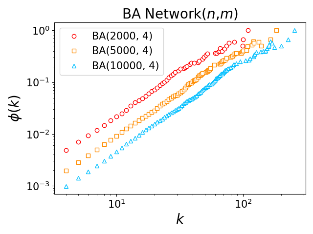
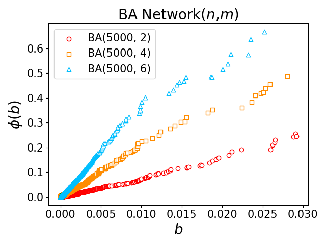
(a)	(b)

Figure 1: The value of RCC in BA network $G(n,m)$, where $n$ is the number of nodes and $m$ is the number of new edges introduced at each step. (a) Log-log plot of $\phi(k)$ versus degree centrality. (b) The plot of $\phi(b)$ versus betweenness centrality. As the maximum value of betweenness centrality is too large, for displaying the feature, the top one percent of nodes has been removed from the plot.

II Centrality in scale-free networks

The most prominent characteristic of a scale-free (SF) network is its degree distribution, which follows a power law, $p(k)\sim k^{-\gamma}$. This feature is widely recognized as key to identifying SF networks Cohen and Havlin (2010). For BA network, it is a growth model with preferential linking, and yields a power-law degree distribution with $\gamma=3$ Barabási and Albert (1999) . Unlike degree centrality (DC), which describes a node’s importance based on its number of edges, betweenness centrality (BC) characterizes the influence of a node on communication between each pair of vertices, making it a useful tool in network topology analysis. Goh et al have shown that the BC (or “load”) distribution in a SF network obeys power-law with exponent $\delta$ Goh et al. (2001): $p(b)\sim b^{-\delta}$ (Since BC is relatively continuous, we here only obtain the cumulative distribution of $P(b)\sim b^{1-\delta}$). There is a strong connection between DC and BC. Especially in SF networks, nodes with high degree values typically create an obvious core structure, which is in the center of communication between nodes Ma and Mondragón (2015). By setting $b_{k}$ as the average BC value of each group of nodes with degree k, the power exponential relation can be obtained Goh et al. (2001),

$$\begin{split}\ b_{k}\sim k^{\eta}\;.\end{split}$$ (3)

On the basis of eliminating the interference by average value, this relation describes the correlation between DC and BC in scale-free networks. Transforming it into the cumulative distributionVázquez et al. (2002), obtains,

$$\begin{split}\ P_{k}(k)\sim k^{\eta(1-\delta)}\sim k^{(1-\gamma)}\;,\end{split}$$ (4)

which confirms the following scaling relation

$$\begin{split}\ \eta=\dfrac{\gamma-1}{\delta-1}\;.\end{split}$$ (5)

According to Barthélemy Barthélemy (2004), the values of $\delta$ and $\eta$ are not universal and depend on specific details of the networks. However, for $m=1$ in a BA network, it has been shown in a tree network that $\eta=\delta=2$ (BA network is not a tree).

In the previous section we have known that RCC is a power function of DC and a linear function of BC, given by $\phi(k)\sim k^{\beta}$ and $\phi(b)\sim\theta\cdot b$, respectively. Comparing them to the relation (3) leads to,

$$\begin{split}\ \eta\approx\beta\;.\end{split}$$ (6)

It can be checked, as also shown in Fig. 2, that the slopes of two fitted lines are nearly identical in a log-log plot. In SF networks, understanding DC and BC is crucial for understanding the characteristics of networks. From the distribution of centrality to the association between centrality, scholars have been exploring various new features to describe more accurately networks. The emergence of rich-club theory undoubtedly provides a new method to study the association between nodes based on centrality, and brings answers to the macro phenomena of the network.

III Analysis of rich-club coefficient

III.1 RCC and Correlation

In order to verify the curve of RCC in SF networks and explore how the relation between RCC and centrality is generated. We begin by dismantling the network similarly to the k-core method Dorogovtsev et al. (2006), and calculate the connections between nodes at each level. When the richness is DC, the form of RCC is to summarize the number of edges between nodes of different degrees. The number of edges in each group provides the data required for calculating the joint degree distribution, which establishes a relation between RCC and joint distribution. Therefore, we can use this to calculate RCC. The joint degree distribution of any given network is

$$\begin{split}\ p(i,j)=\dfrac{E_{i,j}}{N\left\langle k\right\rangle}\;,\end{split}$$ (7)

where $E_{i,j}$ is the number of edges between nodes with degree $i$ and nodes with degree $j$, $N$ is the number of nodes, and $\left\langle k\right\rangle$ is the average degree of the network. Then we can obtain, $2E_{>k}=\textstyle\sum_{ij}E_{ij}=\textstyle\sum_{ij}N\left\langle k\right\rangle p(i,j),N_{>k}=N\textstyle\sum_{i}p(i)$. Converting the numerator and denominator of $\phi(k)$ into calculating cumulants, we obtain,

$$\begin{split}\ \phi(k)=\frac{{\textstyle\sum_{ij}N\left\langle k\right\rangle p(i,j)}}{N{\textstyle\sum_{i}p(i)}[N{\textstyle\sum_{i}p(i)}-1]}\;.\end{split}$$ (8)

It shows clearly that $\phi(k)$ is a cumulants quantity of the joint degree distribution, and the connection between nodes calculated by $\phi(k)$ can be obtained by the sum of degree-degree correlations. Therefore, RCC is also a method to calculate correlations, with a larger RCC indicating a strong correlation.

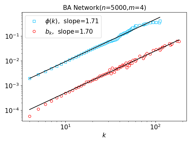
Figure 2: Values of $b_{k}$ and $\phi(k)$ in a BA network. Square points are the value of $\phi(k)$, forming a line with a slope of 1.71; Circular points are the value of $b_{k}$, forming a line with a slope of 1.70. These two lines have similar slopes, which proves the relation (6).

The calculation of joint degree distribution is commonly divided into two cases. One is that in uncorrelated networks, the joint degree distribution can be decomposed as

$$\begin{split}\ p_{unc}(i,j)=\frac{ijp(i)p(j)}{\left\langle k\right\rangle^{2}}\;.\end{split}$$ (9)

In this case, the joint degree distribution is a function of the degree distribution. If $k$ is assumed to be a continuous variable Colizza et al. (2006), in the approximation of $k,k_{max}\to\infty$, L’Hôpital’s rule can give $\phi(k)$ in a simplified version,

$$\begin{split}\ \phi(k)_{unc}\approx\frac{\iint_{k}^{k_{max}}ijp(i)p(j)didj}{N\left\langle k\right\rangle[\int_{k}^{k_{max}}p(i)di]^{2}}\sim\frac{k^{2}}{N\left\langle k\right\rangle}\;.\end{split}$$ (10)

The result shows that the power function also applies to $\phi(k)$ in uncorrelated networks.

For SF networks, the degree-degree correlation has been proved. Krapivsky and Redner (2001). However, the joint degree distribution cannot be simply decomposed and its computation remains a challenge. The analytical expression obtained so far is very complicated Fotouhi and Rabbat (2013); Peköz et al. (2017), and using them will complicate our problems. Therefore, we give up the idea of using the joint distribution to calculate RCC of SF networks. This does not mean we neglect the contribution of the joint degree distribution, which plays a valuable role in helping us understand that RCC represents an accumulation of correlation.

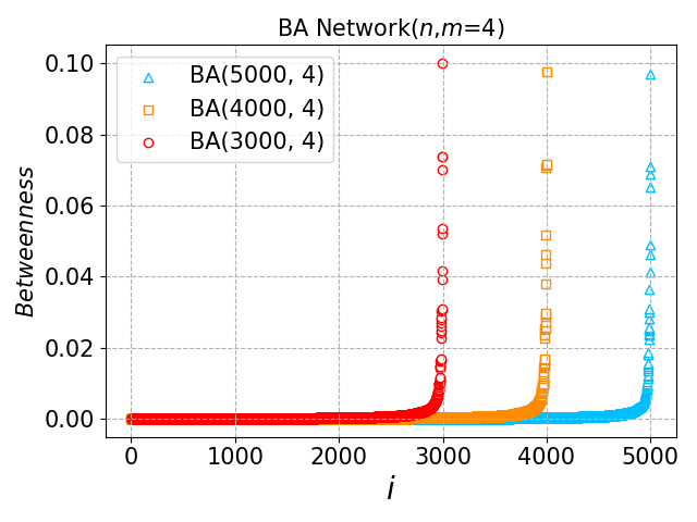
Figure 3: Sequences of betweeness centrality in BA networks. The nodes are sorted by their values of BC. The abscissa is the sequence number, and the ordinate is the corresponding value of BC.

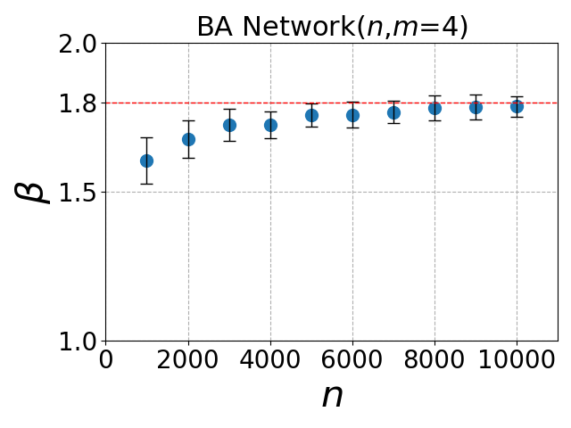
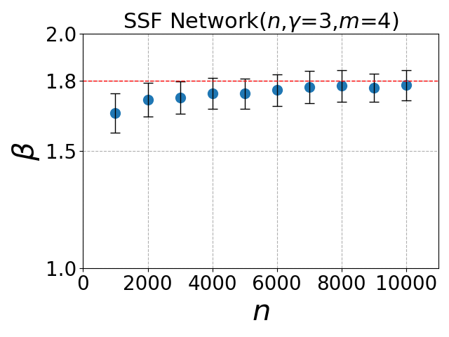
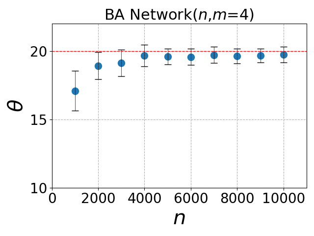
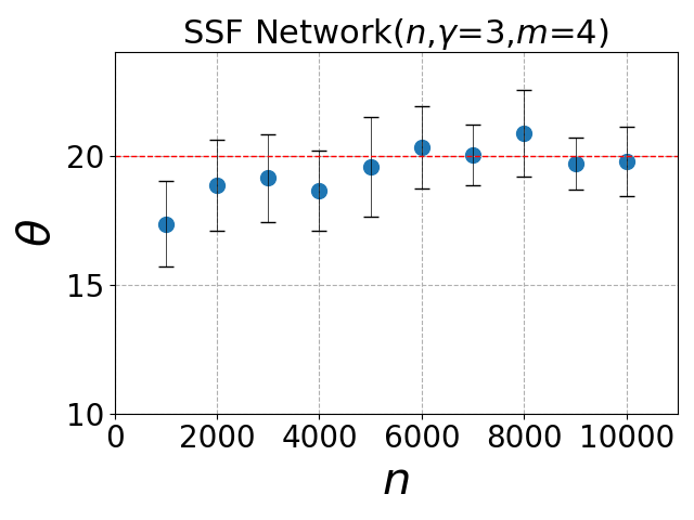
(a)	(b)	(c)	(d)

Figure 4: Values of $\beta$ and $\theta$ in scale-free networks under different $n$, but with the same $\gamma=3$ and $m=4$. Both $\beta$ and $\theta$ converge to a value for large $n$.

III.2 RCC and Centrality Distribution

Our next step is to obtain RCC of a SF network through an evolutionary process. To illustrate it, let’s consider a BA network $G(n,E)$ with $m$ new edges being added at each step. Nodes in the network are ranked by their richness in ascending order, and each node is assigned a sequence number based on its position in the ranking list. After node $i$ is removed, the network density is

$$\begin{split}\ \rho_{>i}=\dfrac{2(E-{\textstyle\sum_{1}^{i}l_{j}})}{(n-i)(n-i-1)}\;.\end{split}$$ (11)

The variable $l_{j}$ represents the number of edges that are removed when node $i$ is cut off from the network. The density calculated using this formula serves as RCC of the network, but its calculation poses a challenge due to the varying values of $l_{j}$ with node deletion at each step. Thus, computing the accurate RCC value is a difficult task. But for our purposes, we want to verify the curve of RCC and analyze its production process. As $l_{j}$ in the BA network approximates $m$, using $l_{j}=m$ directly will not affect our conclusion. In this case, the total number of edges $E={\textstyle\sum_{1}^{n-m}l_{j}}+m$, RCC is given by

$$\begin{split}\ \phi(i)=\frac{2({\textstyle\sum_{i+1}^{n-m}}l_{j}+m)}{(n-i)(n-i-1)}=\frac{2(n-m-i)m}{(n-i)(n-i-1)}\;,\end{split}$$ (12)

when $i<n-m,n\gg m$

$$\begin{split}\ \phi(i)\approx\frac{2m(n-i)}{(n-i)(n-i)}\approx\frac{2m}{n-i}\;,\end{split}$$ (13)

which an inverse proportional function. Our next objective is to discuss the relation between centrality and node sequence, and attempt to obtain RCC of centrality.

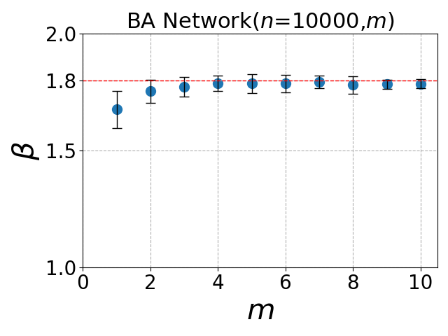
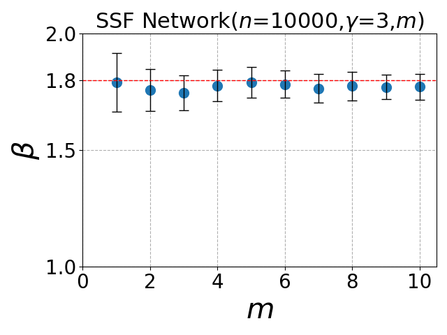
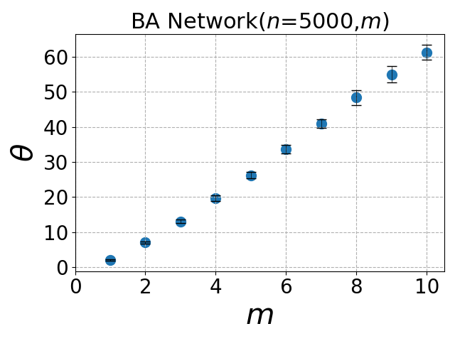
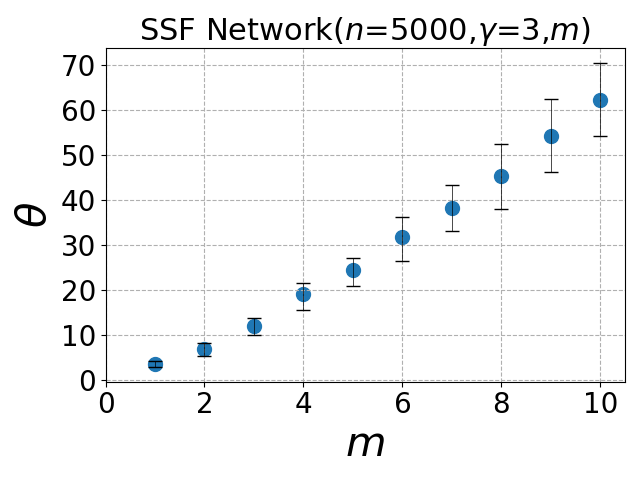
(a)	(b)	(c)	(d)

Figure 5: Values of $\beta$ and $\theta$ in scale-free networks under different $m$ values, but with the same $n$ and $\gamma=3$. Figures (a) and (b) indicate that the value of $\beta$ is near $1.8$. Figures (c) and (d) show that $\theta$ and $m$ have linear correlations.

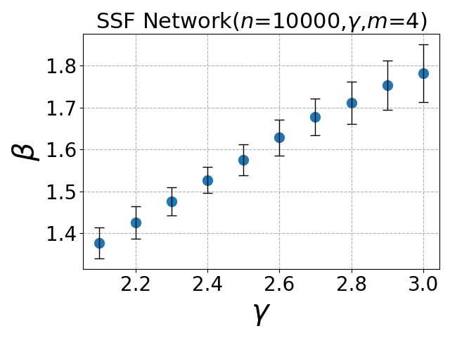
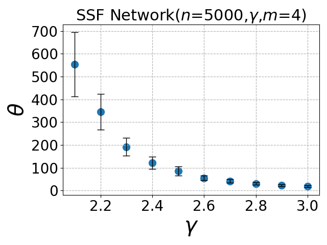
(a)	(b)

Figure 6: Exponent $\beta$ and slope $\theta$ versus $\gamma$ in SSF networks. (a) Linear relation between $\beta$ and $\gamma$. (b) Inverse relation between $\theta$ and $\gamma$.

When the richness is BC, we can see that the curve of BC is also an inverse proportional function, as shown in Fig. 3. The relation between BC and sequence number $i$ is $b_{i}\sim\frac{1}{n-i}$. Compared to formula (13), a linear relation can be obtained: $\phi(b)\sim\theta\cdot b$. It shows that the linear relation of RCC is the result of two inverse proportional functions, with the distribution of BC being the main influencing factor. When the richness is DC, since we calculate the average value of $\phi(k)$ at a given degree, we are unable to reveal the relation between $\phi(k)$ and $k$ through the relation between $k$ and $i$. Instead, calculating $\phi(k)$ requires using $b_{k}\sim k^{\eta}$, which also takes an average result, and ultimately leads to a new relation in the form of $\phi(k)\sim k^{\beta}$. And relation (3) combines two centrality distributions Goh et al. (2001), so $\phi(k)$ is also determined by them. In this section, we have further verified that the power function between RCC and DC, as well as the linear relation between RCC and DC, exist in SF networks. Additionally, we get the conclusion that the distribution of centrality determines the characteristics of the RCC curve. Based on the calculation process, the degree distribution may be the main factor. Therefore, the relation (2) is universal in SF networks. And we can also predict that the values of $\beta$ and $\theta$ in the SF network will be affected by the exponent $\gamma$.

IV The behaviors of exponent $\beta$ and slope $\theta$

After understanding how the curve of RCC is formed, our goal is to explore what affects the values of $\beta$ and $\theta$. We will study the parameters of network construction, which are the most basic data of a network. These include the number of nodes ($n$), the number of new edges ($m$), and the degree distribution exponent($\gamma$) in SF networks. In the numerical calculation, we use two SF models for comparison and verification. One is the BA network, generated through dynamic growth with adjustable parameters $n$ and $m$. For comparison, another network we want to use is a random model. We construct a static scale-free (SSF) network based on the degree sequence following a power-law distribution Hagberg et al. (2020); Bayati et al. (2010). Unlike the BA network, the SSF network does not have a dynamic growth process, and has adjustable $\gamma$ (We set $\gamma$ in the usual range $\left(2,3\right]$). We can multiply the degree sequence $\left\{k_{n}\right\}$ by a factor of $m$ to approximate the network density to that of a BA network. Therefore, the SSF network has a strong randomness, with adjustable parameters $n$, $m$ and $\gamma$.

Initially, we discuss the effect of the change in the number of nodes on the exponent $\beta$ and slope $\theta$. To enable the smoothness of fitting, we base our results on the average outcomes of multiple calculations. As shown in Fig. 4, we construct the BA network and SSF network with the same $m=4$ and $\gamma=3$, and then gradually increase the number of nodes. We can see the values of $\beta$ and $\theta$ rise to convergence as $n$ increases, and conclude that the values of exponent $\beta$ and slope $\theta$ are not affected by the number of nodes in a large SF network. This also verifies that the exponent $\eta$ does not vary with network size Barthélemy (2004). In addition, when $n$ is small, the initial density is large enough to affect the fitted value. As the size increases, the effect diminishes to 0.

In Fig. 5, we have kept $n$ and $\gamma$ constant while setting $m\in\left[1,10\right]$. Our results indicate distinct behaviors between $\beta$ and $\theta$. Specifically, we have found that the exponent $\beta$ is relatively stable across the range of $m$, whereas the slope $\theta$ exhibits a linearly positive correlation with $m$. As $m$ directly affects the density of the network, it is inconsistent with our experience that the fitting value $\beta$ remains constant with changes in $m$. This may be the fact that $m$ is too small for $n$ in the usual range, resulting in little change in initial density. Different from the case in exponent $\beta$, the value of $\theta$ is impacted by the inclusion of $m$ in the numerator of $\phi(r)$, resulting in a proportional increase between $\theta$ and $m$. However, due to the limitation of fitting accuracy, we have only explained the trend of the curve without discussing the obtained numerical result in detail. But our numerical results also make sense, they show $\beta\approx 1.8,\delta\approx 2.1$, which is in the proximity of the previous one. Goh et al. (2001).

Finally, we change the degree distribution exponent $\gamma$ in SSF network. Fig. 6 shows when $\gamma$ increases in the interval $\left(2,3\right]$, $\beta$ and $\theta$ also exhibit different behaviors. $\beta$ and $\gamma$ increase together, they tend to increase linearly; $\theta$ gradually decreases to convergence as $\gamma$ increases. The exponent $\gamma$ changes the value of the degree sequence $\left\{k_{n}\right\}$ and affects the distribution of BC in SSF networks. However, the precise manner in which $\gamma$ affects the details of the network remains unclear. We cannot find the reason that $\beta$ and $\gamma$ are linearly dependent, and why $\theta$ converges. It is a very worthy problem to discuss, which may require a deeper understanding of node centrality.

V Summary and Conclusions

In the previous work, we have studied the behavior of RCC in scale-free networks, and found that RCC is an important quantity to describe the characteristics of scale-free networks. It can give the connection between rich nodes through the centrality, and form a association process with the distribution of centrality. The numerical results show that the relation between RCC and DC is a power function $\phi(k)\sim k^{\beta}$, and the relation between RCC and BC is a linear function $\phi(b)\sim\theta\cdot b$. Compared to the existing centrality features in scale-free networks, we also find that the exponents $\beta$ and $\eta$ are close in value. In addition, RCC provides a way of calculating correlation, which is represented by the form of cumulative joint distribution. For example, when richness is degree, a larger RCC means not only greater density but also greater degree-degree correlation among a group of nodes. In order to explore how the RCC is formed, we first try to calculate $\phi(k)$ with the aid of the joint degree distribution. But we did not succeed, because the current results of the joint degree distribution do not simplify our calculations, it cannot help us find the factors affecting the curve. Then we changed the method and tried to calculate RCC in scale-free networks by removing nodes. In BA networks, we calculate the result of RCC and node sequence, and under the approximation of removing $m$ edges in every step, the simplified relation is $\phi(r)\approx\frac{2m}{n-r}$. This is a general result, where $r$ can be any sequence of centrality (or other data Cinelli (2019)). The sequence of BC is used, and it shows that the sorting of BC is an inverse proportional function. So the linear function of $\phi(b)$ is the result of two inverse proportional functions. Because $\phi(k)$ is the average result under the same degree value, we use relation (3) to calculate and get the power function. It can be concluded that the relation between RCC and centrality is dominated by the distribution of centrality, and the sequence of centrality significantly affects the curve of RCC. As such, understanding the characteristics of RCC is an import component of comprehending scale-free networks.

We have also discussed what affect the values of $\beta$ and $\theta$ in terms of network construction parameters. In order to compare the results of BA networks, we use a static scale-free network with strong randomness, whose degree distribution is randomly generated for a given exponent $\gamma$. In many simulations, the results show that $\beta$ and $\gamma$ increase together, $\theta$ increases with $m$ and decreases to convergence as $\gamma$ increases. To understand why $\beta$ and $\theta$ behave this way, we need to have a deeper understanding of centrality and explore how the change of $\gamma$ changes the network structure. Moreover, the study of joint distribution in scale-free networks can also help us further understand the behavior of RCC.

Acknowledgements: This work was supported in part by the Fundamental Research Funds for the Central Universities, China (Grant No. CCNU19QN029), the National Natural Science Foundation of China (Grant No. 61873104), and the 111 Project 2.0, with Grant No. BP0820038.

References

- Opsahl et al. (2008) T. Opsahl, V. Colizza, P. Panzarasa, and J. J. Ramasco, Physical review letters 101, 168702 (2008).
- Zhao et al. (2018) L. Zhao, W. Li, and Y. Zhu, in Journal of Physics: Conference Series, Vol. 1113 (IOP Publishing, 2018) p. 012010.
- Zhou and Mondragón (2004) S. Zhou and R. J. Mondragón, IEEE communications letters 8, 180 (2004).
- Aghaee et al. (2020) Z. Aghaee, H. A. Beni, S. Kianian, and M. Vahidipour, in 2020 6th International Conference on Web Research (ICWR) (IEEE, 2020) pp. 119–125.
- Ansell et al. (2016) C. Ansell, R. Bichir, and S. Zhou, Connections 36, 20 (2016).
- Dong et al. (2015) Y. Dong, J. Tang, N. V. Chawla, T. Lou, Y. Yang, and B. Wang, PloS one 10, e0119446 (2015).
- Vaquero and Cebrian (2013) L. M. Vaquero and M. Cebrian, Scientific reports 3, 1 (2013).
- Wei et al. (2018) Y. Wei, W. Song, C. Xiu, and Z. Zhao, Applied Geography 96, 77 (2018).
- Li and Cai (2007) W. Li and X. Cai, Physica A: Statistical Mechanics and its Applications 382, 693 (2007).
- Zhang and Ng (2021) Y. Zhang and S. T. Ng, Physica A: Statistical Mechanics and its Applications 584, 126377 (2021).
- Zhu et al. (2021) R. Zhu, Y. Wang, D. Lin, M. Jendryke, M. Xie, J. Guo, and L. Meng, Cities 114, 103198 (2021).
- Van Den Heuvel and Sporns (2011) M. P. Van Den Heuvel and O. Sporns, Journal of Neuroscience 31, 15775 (2011).
- Ball et al. (2014) G. Ball, P. Aljabar, S. Zebari, N. Tusor, T. Arichi, N. Merchant, E. C. Robinson, E. Ogundipe, D. Rueckert, A. D. Edwards, et al., Proceedings of the National Academy of Sciences 111, 7456 (2014).
- Griffa and Van den Heuvel (2022) A. Griffa and M. P. Van den Heuvel, Dialogues in clinical neuroscience (2022).
- Jiang and Zhou (2008) Z.-Q. Jiang and W.-X. Zhou, New Journal of Physics 10, 043002 (2008).
- Berahmand et al. (2018) K. Berahmand, N. Samadi, and S. M. Sheikholeslami, International Journal of Modern Physics B 32, 1850142 (2018).
- Cinelli et al. (2017) M. Cinelli, G. Ferraro, and A. Iovanella, Complexity 2017 (2017).
- Colizza et al. (2006) V. Colizza, A. Flammini, M. A. Serrano, and A. Vespignani, Nature physics 2, 110 (2006).
- Hein et al. (2006) O. Hein, M. Schwind, and W. König, Wirtschaftsinformatik 48, 267 (2006).
- Barabási and Albert (1999) A.-L. Barabási and R. Albert, science 286, 509 (1999).
- Cohen and Havlin (2010) R. Cohen and S. Havlin, Complex networks: structure, robustness and function (Cambridge university press, 2010).
- Goh et al. (2001) K.-I. Goh, B. Kahng, and D. Kim, Physical review letters 87, 278701 (2001).
- Ma and Mondragón (2015) A. Ma and R. J. Mondragón, PloS one 10, e0119678 (2015).
- Vázquez et al. (2002) A. Vázquez, R. Pastor-Satorras, and A. Vespignani, Physical Review E 65, 066130 (2002).
- Barthélemy (2004) M. Barthélemy, The European physical journal B 38, 163 (2004).
- Dorogovtsev et al. (2006) S. N. Dorogovtsev, A. V. Goltsev, and J. F. F. Mendes, Physical review letters 96, 040601 (2006).
- Krapivsky and Redner (2001) P. L. Krapivsky and S. Redner, Physical Review E 63, 066123 (2001).
- Fotouhi and Rabbat (2013) B. Fotouhi and M. G. Rabbat, The European Physical Journal B 86, 1 (2013).
- Peköz et al. (2017) E. Peköz, A. Röllin, and N. Ross, Advances in Applied Probability 49, 368 (2017).
- Hagberg et al. (2020) A. Hagberg, D. Schult, and P. Swart, Release 3, b1 (2020).
- Bayati et al. (2010) M. Bayati, J. H. Kim, and A. Saberi, Algorithmica 58, 860 (2010).
- Cinelli (2019) M. Cinelli, Journal of Complex Networks 7, 702 (2019).