Asymptotically compatible energy and dissipation law of the nonuniform L2-$1_{\sigma}$ scheme for time fractional Allen-Cahn model

Abstract

We build an asymptotically compatible energy of the variable-step L2-$1_{\sigma}$ scheme for the time-fractional Allen-Cahn model with the Caputo’s fractional derivative of order $\alpha\in(0,1)$, under a weak step-ratio constraint $\tau_{k}/\tau_{k-1}\geq r_{\star}(\alpha)$ for $k\geq 2$, where $\tau_{k}$ is the $k$-th time-step size and $r_{\star}(\alpha)\in(0.3865,0.4037)$ for $\alpha\in(0,1)$. It provides a positive answer to the open problem in [J. Comput. Phys., 414:109473], and, to the best of our knowledge, it is the first second-order nonuniform time-stepping scheme to preserve both the maximum bound principle and the energy dissipation law of time-fractional Allen-Cahn model. The compatible discrete energy is constructed via a novel discrete gradient structure of the second-order L2-$1_{\sigma}$ formula by a local-nonlocal splitting technique. It splits the discrete fractional derivative into two parts: one is a local term analogue to the trapezoid rule of the first derivative and the other is a nonlocal summation analogue to the L1 formula of Caputo derivative. Numerical examples with an adaptive time-stepping strategy are provided to show the effectiveness of our scheme and the asymptotic properties of the associated modified energy.

Keywords:   time-fractional Allen-Cahn model, discrete gradient structure, discrete energy dissipation law, maximum bound principle, asymptotic compatibility
AMS subject classiffications.   65M12, 65M06, 35Q99, 74A50

1 Introduction

This paper continues to discuss the second-order nonuniform L2-$1_{\sigma}$ scheme in [21] for the time fractional Allen-Cahn (TFAC) model [3, 5, 17, 24, 29, 31],

$$\partial_{t}^{\alpha}\Phi=-\mu\quad\text{with}\quad\mu=\tfrac{\delta E}{\delta\Phi}=f(\Phi)-\epsilon^{2}\Delta\Phi,$$ (1.1)

where $\Phi$ is the phase variable and $E$ is the Ginzburg-Landau type energy functional

$$E[\Phi]:=\int_{\Omega}\Big{(}\frac{\epsilon^{2}}{2}\left|\nabla\Phi\right|^{2}+F(\Phi)\Big{)}\,\mathrm{d}\mathbf{x}\quad\text{with the potential $F(\Phi)=\frac{1}{4}\left(\Phi^{2}-1\right)^{2}$}.$$ (1.2)

The variable $\Phi$ represents the concentration difference in a binary system on the domain $\Omega\subseteq\mathbb{R}^{2}$ and $\epsilon>0$ is an interface width parameter. The notation $\partial_{t}^{\alpha}:={}_{0}^{C}\!D_{t}^{\alpha}$ represents the Caputo’s fractional derivative of order $\alpha\in(0,1)$ with respect to $t$, defined by

$$(\partial_{t}^{\alpha}v)(t):=\int_{0}^{t}\omega_{1-\alpha}(t-s)v^{\prime}(s)\,\mathrm{d}{s}\quad\text{with $\omega_{\beta}(t):=t^{\beta-1}/\Gamma(\beta)$ for $\beta>0$.}$$ (1.3)

As the fractional order $\alpha\rightarrow 1^{-}$, the TFAC model (1.1) is asymptotically compatible with the classical Allen-Cahn (AC) model [2, 4],

$$\partial_{t}\Phi=-\mu\quad\text{with}\quad\mu=\tfrac{\delta E}{\delta\Phi}.$$ (1.4)

As is well known, the AC model preserves the maximum bound principle

$$|\Phi(\mathbf{x},t)|\leq{1}\;\text{for $t>0$}\quad\text{if}\quad|\Phi(\mathbf{x},0)|\leq{1},$$ (1.5)

and the energy dissipation law

$$\frac{\,\mathrm{d}E}{\,\mathrm{d}t}+\big{\|}\mu\big{\|}^{2}=0\quad\text{for $t>0$},$$ (1.6)

where the $L^{2}$ norm $\left\|u\right\|:=\sqrt{(u,u)}$ with the inner product $\left(u,v\right):=\int_{\Omega}uv\,\mathrm{d}\mathbf{x}$ for $u,v\in L^{2}(\Omega).$

In recent years, the TFAC model (1.1) has received extensive attentions and researches in accurately describing anomalous diffusion problems and developing efficient numerical methods to capture the long-time coarsening dynamics [3, 5, 7, 6, 10, 14, 17, 21, 24, 25, 26, 29, 31]. A very interesting problem is whether the TFAC model (1.1) also inherits the maximum bound principle (1.5) and the energy law (1.6) in an appropriate nonlocal form. Tang, Yu and Zhou [29] established the maximum bound principle and derived a global energy dissipation law. Quan, Tang and Yang proposed two nonlocal energy decaying laws for the time-fractional phase field models in [26], including a time-fractional energy dissipation law $\left(\partial_{t}^{\alpha}E\right)(t)\leq 0$ for $t>0$, and a weighted energy dissipation law, $\frac{\,\mathrm{d}E_{\omega}}{\,\mathrm{d}t}\leq 0$ for $t>0$ where $E_{\omega}(t):=\int_{0}^{1}\omega(s)E(st)\,\mathrm{d}s$ is a nonlocal weighted energy. Du, Yang and Zhou [3] investigated the well-posedness and the regularity of solution, and showed that the solution satisfies $\left\|\partial_{t}^{\alpha}\Phi\right\|_{L^{p}(0,T;L^{2})}+\left\|\Delta\Phi\right\|_{L^{p}(0,T;L^{2})}\leq C$ for any $p\in[2,2/\alpha)$ if the initial data $\Phi_{0}\in H^{1}_{0}(\Omega)$. They also discretized the fractional derivative by backward Euler convolution quadrature and developed some unconditionally solvable and stable time stepping schemes of order $O(\tau^{\alpha})$, such as a convex splitting scheme, a weighted convex splitting scheme and a linear weighted stabilized scheme. A fractional energy dissipation law was also obtained in [3] and the discrete energy dissipation laws (in a weighted average sense) were derived for two weighted schemes on the uniform time mesh. Recently, Hou and Xu [5, 7, 6] split the nonlocal time-fractional derivatives, including the L1-type, L2-$1_{\sigma}$ and L2 schemes, to local and nonlocal terms for time-fractional phase field equations, and treated the derived nonlocal term with the SAV technique, so that the resulting modified discrete energy decays with respect to time.

Naturally, we hope that the energy dissipation law of the TFAC model is asymptotically compatible with the energy dissipation law (1.6) of the AC equation (1.4), just as the TFAC model (1.1) is asymptotically compatible with the AC equation (1.4). By reformulating the Caputo’s form (1.1) of the TFAC model into the Riemann-Liouville form, one can follow the arguments [22, Section 1] to obtain the following variational energy dissipation law

$$\frac{\,\mathrm{d}E_{\alpha}}{\,\mathrm{d}t}+\frac{1}{2}\omega_{\alpha}(t)\big{\|}\mu\big{\|}^{2}-\frac{1}{2}\int_{0}^{t}\omega_{\alpha-1}(t-s)\left\|\mu(t)-\mu(s)\right\|^{2}\,\mathrm{d}{s}=0\quad\text{for $t>0$,}$$ (1.7)

with the variational energy

$$E_{\alpha}[\Phi]:=E[\Phi]+\frac{1}{2}\int_{0}^{t}\omega_{\alpha}(t-s)\big{\|}\mu(s)\big{\|}^{2}\,\mathrm{d}{s}.$$ (1.8)

As remarked, the variational energy dissipation law (1.7) is asymptotically compatible with the energy dissipation law (1.6) of the AC equation (1.4). In recent works [23, 12, 22], the discrete gradient structures of some variable-step L1-type formulas of the Caputo and Riemann-Liouville fractional derivatives were constructed via the so-called discrete orthogonality convolution kernels. The associated discrete energy dissipation laws of the corresponding schemes for time-fractional gradient flows were shown to be asymptotically compatible with the original energy law of their integer-order counterparts. As seen, the variational energy (1.8) and its discrete versions in [23, 12, 22] are always incompatible with the original (discrete) energy, in the fractional order limit $\alpha\rightarrow 1^{-}$, due to the presence of the history effect in the Riemann-Liouville integral form.

In a recent interesting work [25], Quan et al. proposed the following nonlocal-in-time modified energy (in our notations), formulated as the summation of the original energy $E[\Phi]$ and a new accumulation term due to the memory effect from time fractional derivative,

$$\mathcal{E}_{\alpha}[\Phi]:=E[\Phi]+\frac{\omega_{1-\alpha}(t)}{2}\left\|\Phi(t)-\Phi(0)\right\|^{2}-\frac{1}{2}\int_{0}^{t}\omega_{-\alpha}(t-s)\left\|\Phi(t)-\Phi(s)\right\|^{2}\,\mathrm{d}{s}.$$ (1.9)

It is remarkable that this decreasing upper bound functional decays with respect to time and is asymptotically compatible with the original energy $E[\Phi]$ in the fractional order limit $\alpha\rightarrow 1^{-}$. The associated modified energy and energy dissipation laws at discrete time levels were derived in [25] for several L1 and L2-type implicit-explicit stabilized schemes on the uniform time mesh in solving time-fractional gradient flow problems. The modified discrete energies of these time-stepping schemes are incompatible (in the sense of $\alpha\rightarrow 1^{-}$) with their integer-order counterparts, see [25, Theorems 4.1-4.2 and 5.2], although they always coincide with the original energy at the initial time $t=0$ and as the time $t$ tends to $\infty$ (the steady state).

As observed from the extensive experiments in [5, 7, 6, 23, 12, 17, 21, 22, 24, 25, 26, 29, 31], the time-fractional gradient flow models admit multiple time scales in the long-time coarsening dynamics approaching the steady state. Thus an adaptive time-stepping strategy seems more suitable to capture the multiscale behaviors and to save computational cost by choosing proper time-step sizes at different time periods. It is natural to require theoretically reliable time-stepping methods on general setting of time-step variations. We consider a time mesh $0=t_{0}<t_{1}<\cdots<t_{k}<\cdots<t_{N}=T$ with the time-step sizes $\tau_{k}:=t_{k}-t_{k-1}$ for $1\leq{k}\leq{N}$ and the time-step ratios $r_{k}:=\tau_{k}/\tau_{k-1}$ for $2\leq k\leq N$ (the step-ratio notation $\rho_{k}=1/r_{k+1}$ was used in previous works [20, 21]).

The nonuniform L2-$1_{\sigma}$ formula [20] of the Caputo derivative was applied in [21] to build a second-order maximum-bound-principle-preserving scheme for the TFAC model (1.1); however, no energy dissipation law of the second-order L2-$1_{\sigma}$ scheme has been established due to the lack of technology to establish the positive definiteness (or discrete gradient structure) of the discrete derivative on general nonuniform time meshes. Very recently, Quan and Wu [27] made a key progress on this issue by establishing the positive definiteness of the L2-$1_{\sigma}$ formula on general nonuniform meshes with a mild step-ratio restriction $r_{k}\geq 0.475329$ for $k\geq 2$. They also proved the $H^{1}$-stability of the L2-$1_{\sigma}$ time-stepping scheme for linear subdiffusion equations. Nonetheless, the positive definiteness of the discrete fractional operator should be inadequate to build an asymptotically compatible discrete energy for the TFAC model (1.1).

In this paper, we revisit the variable-step L2-$1_{\sigma}$ scheme for the TFAC model (1.1) and provide a positive answer to the unsolved problem raised in [21]. Our contribution is two folds:

• A new local-nonlocal splitting is adopted to split the L2-$1_{\sigma}$ formula into two parts: one is a local term analogue to the trapezoid rule of the first derivative and the other is a nonlocal summation analogue to the L1 formula of Caputo derivative. Then a novel discrete gradient structure (DGS) of the L2-$1_{\sigma}$ formula is constructed under an updated step-ratio constraint, that is $r_{k}\geq r_{\star}(\alpha)$ for $k\geq 2$ where $r_{\star}(\alpha)\in(0.3865,0.4037)$ for $\alpha\in(0,1)$, which is a little weaker than those in previous studies [20, 21, 27].

• An asymptotically compatible energy and the associated energy dissipation law of the variable-step L2-$1_{\sigma}$ scheme are established for the TFAC model (1.1). To the best of our knowledge, it is the first second-order nonuniform time-stepping scheme to preserve both the maximum bound principle and an asymptotically compatible energy dissipation law of the TFAC model.

This paper is organized as follows. Section 2 describes the L2-$1_{\sigma}$ formula and constructs a new discrete gradient structure by using a novel local-nonlocal splitting. An asymptotically compatible discrete energy and the associated energy law of the L2-$1_{\sigma}$ implicit time-stepping scheme are established in Section 3 for the TFAC model. Some numerical experiments are included in the last section to support our theoretical results.

2 Discrete gradient structure of L2-1_σ formula

Set an off-set parameter $\theta:={\alpha}/{2}$ and $t_{k-\theta}:=\theta t_{k-1}+(1-\theta)t_{k}$. For any grid function $\{w^{k}\}_{k=0}^{N}$, denote $\triangledown_{\tau}w^{k}:=w^{k}-w^{k-1}$, $\partial_{\tau}w^{k-\frac{1}{2}}:=\triangledown_{\tau}w^{k}/\tau_{k}$ and the operator $w^{k-\theta}:=\theta w^{k-1}+(1-\theta)w^{k}$ for $k\geq 1$. For simplicity of presentation, we will always use the following notations

$$\varpi_{n}(t):=-\omega_{2-\alpha}(t_{n-\theta}-t)\quad\text{and}\quad\varpi_{n}^{\prime}(t):=\omega_{1-\alpha}(t_{n-\theta}-t)\quad\text{for $0\leq t\leq t_{n-\theta}$}.$$

2.1 Variable-step L2-1_σ formula

Let $\Pi_{1,k}v$ be the linear interpolant of a function $v$ with respect to the two nodes $t_{k-1}$ and $t_{k}$, and let $\Pi_{2,k}v$ denote the quadratic interpolant with respect to $t_{k-1}$, $t_{k}$ and $t_{k+1}$. One has

$$\left(\Pi_{1,k}v\right)^{\prime}(t)=\frac{\triangledown_{\tau}v^{k}}{\tau_{k}}\;\;\text{and}\;\;\left(\Pi_{2,k}v\right)^{\prime}(t)=\frac{\triangledown_{\tau}v^{k}}{\tau_{k}}+\frac{2(t-t_{k-1/2})}{\tau_{k+1}(\tau_{k}+\tau_{k+1})}\big{(}\triangledown_{\tau}v^{k+1}-r_{k+1}\triangledown_{\tau}v^{k}\big{)}.$$

The L2-1_σ formula [1, 20, 21, 27] of Caputo derivative (1.3) can be obtained by employing a quadratic interpolant in each subinterval $[t_{k-1},t_{k}]$ for $1\leq k\leq n-1$ and a linear interpolant in the final subinterval $[t_{n-1},t_{n-\theta}]$. That is

$$(\partial^{\alpha}_{\tau}v)^{n-\theta} :=\int_{t_{n-1}}^{t_{n-\theta}}\varpi_{n}^{\prime}(s)\left(\Pi_{1,n}v\right)^{\prime}(s)\,\mathrm{d}{s}+\sum_{k=1}^{n-1}\int_{t_{k-1}}^{t_{k}}\varpi_{n}^{\prime}(s)\left(\Pi_{2,k}v\right)^{\prime}(s)\,\mathrm{d}{s}$$ (2.1)

$$=a^{(n)}_{0}\triangledown_{\tau}v^{n}+\sum_{k=1}^{n-1}\Big{(}a^{(n)}_{n-k}\triangledown_{\tau}v^{k}+\frac{\triangledown_{\tau}v^{k+1}-r_{k+1}\triangledown_{\tau}v^{k}}{r_{k+1}(1+r_{k+1})}\zeta^{(n)}_{n-k}\Big{)},$$

where $a_{n-k}^{(n)}$ and $\zeta_{n-k}^{(n)}$ are positive coefficients defined by

$$a^{(n)}_{n-k}:=\frac{1}{\tau_{k}}\int_{t_{k-1}}^{\min\{t_{k},t_{n-\theta}\}}\varpi_{n}^{\prime}(s)\,\mathrm{d}{s}\quad\text{for $1\leq k\leq n$},$$ (2.2)

$$\zeta^{(n)}_{n-k}:=\frac{2}{\tau_{k}^{2}}\int_{t_{k-1}}^{t_{k}}(s-t_{k-\frac{1}{2}})\varpi_{n}^{\prime}(s)\,\mathrm{d}{s}\quad\text{for $1\leq k\leq n$}.$$ (2.3)

2.2 Discrete gradient structure

Notice that if $\alpha\rightarrow 1^{-}$, then $\omega_{2-\alpha}(t)\to 1$ whereas $\omega_{1-\alpha}(t)\to 0$, uniformly for $t$ in any compact subinterval of the open half-line $(0,\infty)$. Thus, $a^{(n)}_{0}=\omega_{2-\alpha}((1-\theta)\tau_{n})/\tau_{n}\to 1/\tau_{n}$ whereas $a^{(n)}_{n-k}\to 0$ and $\zeta^{(n)}_{n-k}\to 0$ for $1\leq k\leq n-1$. It follows that

$$(\partial^{\alpha}_{\tau}v)^{n-\theta}\;\;\to\;\;\partial_{\tau}v^{n-\frac{1}{2}}\quad\text{as $\alpha\rightarrow 1^{-}$,}$$

so that the L2-1_σ formula (2.1) tends to the Crank-Nicolson approximation at the offset point $t_{n-1/2}$ of the first time derivative. This asymptotic property inspires us to split the discrete fractional derivative (2.1) into two parts,

$$(\partial^{\alpha}_{\tau}v)^{n-\theta}\triangleq \,\underbrace{\frac{\alpha}{2-\alpha}a_{0}^{(n)}\triangledown_{\tau}v^{n}}+\underbrace{\sum_{k=1}^{n}\hat{a}_{n-k}^{(n)}\triangledown_{\tau}v^{k}}\quad\text{for $n\geq 1$},$$ (2.4)

$$\,\hskip 28.45274ptJ_{CN}^{n}\hskip 56.9055ptJ_{L1}^{n}$$

where the discrete convolution kernels $\hat{a}_{n-k}^{(n)}$ are defined by, $\hat{a}_{0}^{(1)}:=\frac{2(1-\alpha)}{2-\alpha}a_{0}^{(1)}$ and

$$\hat{a}^{(n)}_{n-k}:=\begin{cases}\frac{2(1-\alpha)}{2-\alpha}a^{(n)}_{0}+\frac{1}{r_{n}(1+r_{n})}\zeta^{(n)}_{1},&\text{for $k=n$, $n\geq 2$}\\[4.30554pt] a^{(n)}_{n-k}+\frac{1}{r_{k}(1+r_{k})}\zeta^{(n)}_{n-k+1}-\frac{1}{1+r_{k+1}}\zeta^{(n)}_{n-k},&\text{for $2\leq k\leq n-1$, $n\geq 3$}\\[4.30554pt] a^{(n)}_{n-1}-\frac{1}{1+r_{2}}\zeta^{(n)}_{n-1},&\text{for $k=1$, $n\geq 2$.}\end{cases}$$ (2.5)

It is seen that the local part $J_{CN}^{n}$ is similar to the Crank-Nicolson approximation of first time derivative and the second part $J_{L1}^{n}$ represents an L1-type formula of Caputo derivative (1.3). In general, the coefficient of $J_{CN}^{n}$ should be properly large so that $J_{CN}^{n}\rightarrow\partial_{\tau}v^{n-\frac{1}{2}}$ and $J_{L1}^{n}\rightarrow 0$ as the fractional order $\alpha\rightarrow 1^{-}$, and it should also be properly small so that the remaining part $J_{L1}^{n}$ admits a discrete gradient structure under a weak step-ratio constraint.

We will apply the splitting formulation (2.4) to derive a new discrete gradient structure of the L2-1_σ formula (2.1), which plays an important role in establishing the discrete energy dissipation law of our numerical scheme. As we will see in Lemma 2.2 and Theorem 2.1, the current choice $\frac{\alpha}{2-\alpha}a_{0}^{(n)}$ in the local part $J_{CN}^{n}$ would be subtle and key to obtain the minimum allowable lower bound $r_{\star}(\alpha)$ of the time-step ratios for an asymptotically compatible discrete energy of the corresponding L2-1_σ time-stepping scheme.

Lemma 2.1.

Let $r_{\star}=r_{\star}(\alpha)$ be the unique positive root of the equation

$$h(r_{\star},\alpha):=2\sqrt{\frac{2(1-\alpha/2)r_{\star}}{1+\alpha+(1-\alpha/2)r_{\star}}+\frac{r_{\star}}{1+r_{\star}}}+3-\frac{1}{r_{\star}^{2}(1+r_{\star})}=0\quad\text{for $\alpha\in(0,1)$.}$$

It holds that $0.3865\approx r_{\star}(0)<r_{\star}(\alpha)<r_{\star}(1)\approx 0.4037$  for $\alpha\in(0,1)$.

Proof.

It is not difficult to find that

$$\partial_{r_{\star}}h= \,\Big{(}\frac{2r_{\star}}{\frac{2+2\alpha}{2-\alpha}+r_{\star}}+\frac{r_{\star}}{1+r_{\star}}\Big{)}^{-\frac{1}{2}}\left[\frac{4}{(\frac{2+2\alpha}{2-\alpha}+r_{\star})^{2}}\frac{1+\alpha}{2-\alpha}+\frac{1}{(1+r_{\star})^{2}}\right]+\frac{3r_{\star}+2}{r_{\star}^{3}(1+r_{\star})^{2}}>0,$$

$$\partial_{\alpha}h= \,-\frac{12r_{\star}}{(2-\alpha)^{2}(\frac{2+2\alpha}{2-\alpha}+r_{\star})^{2}}\Big{(}\frac{2r_{\star}}{\frac{2+2\alpha}{2-\alpha}+r_{\star}}+\frac{r_{\star}}{1+r_{\star}}\Big{)}^{-\frac{1}{2}}<0\quad\text{for $\alpha\in(0,1)$ and $r_{\star}>0$.}$$

Due to the fact $h(1/4,\alpha)h(1/2,\alpha)<0$ for any $\alpha\in(0,1)$, the equation $h(r_{\star},\alpha)=0$ has a unique positive root $r_{\star}=r_{\star}(\alpha)\in(1/4,1/2)$. Thanks to the implicit function theorem, one has $r_{\star}^{\prime}(\alpha)>0$ and the root $r_{\star}(\alpha)$ is increasing with respect to $\alpha\in(0,1)$. That is, $r_{\star}(0)<r_{\star}(\alpha)<r_{\star}(1)$. Then we complete the proof by solving the two equations $h(r_{\star}(0),0)=0$ and $h(r_{\star}(1),1)=0$ numerically and find that $r_{\star}(0)\approx 0.3865$ and $r_{\star}(1)\approx 0.4037$. ∎

Lemma 2.2.

For the discrete kernels $\hat{a}_{n-k}^{(n)}$ in (2.5), define the auxiliary convolution kernels

$$A_{0}^{(n)}:=2\hat{a}_{0}^{(n)}\quad\text{and}\quad A_{n-k}^{(n)}:=\hat{a}_{n-k}^{(n)}\quad\text{for $1\leq k\leq n-1$.}$$ (2.6)

For $r_{\star}=r_{\star}(\alpha)$ defined in Lemma 2.1, assume that the adjacent time-step ratios $r_{k}$ fulfill

$$r_{k}\geq r_{\star}(\alpha)\quad\text{for $k\geq 2$.}$$ (2.7)

Then the auxiliary convolution kernels $A_{n-k}^{(n)}$ satisfy

• $A^{(n)}_{n-k-1}>A^{(n)}_{n-k}>0$  for $1\leq k\leq n-1$ $(n\geq 2)$;

• $A^{(n-1)}_{n-1-k}>A_{n-k}^{(n)}$  for $1\leq k\leq n-1$ $(n\geq 2)$;

• $A^{(n-1)}_{n-2-k}-A^{(n-1)}_{n-1-k}>A^{(n)}_{n-k-1}-A^{(n)}_{n-k}$  for $1\leq k\leq n-2$ $(n\geq 3)$.

Proof.

See the lengthy but technical proof in Section 4. ∎

Theorem 2.1.

Under the step-ratio constraint (2.7), it holds that

$$2(\triangledown_{\tau}v^{n})(\partial^{\alpha}_{\tau}v)^{n-\theta}=\mathcal{G}[\triangledown_{\tau}v^{n}]-\mathcal{G}[\triangledown_{\tau}v^{n-1}]+\mathcal{R}[\triangledown_{\tau}v^{n}]+\frac{2\alpha a_{0}^{(n)}}{2-\alpha}(\triangledown_{\tau}v^{n})^{2}\quad\text{for $n\geq 1$,}$$

where the nonnegative functionals $\mathcal{G}$ and $\mathcal{R}$ are defined by

$$\mathcal{G}[w^{n}] :=\sum_{j=1}^{n-1}\big{(}A^{(n)}_{n-j-1}-A^{(n)}_{n-j}\big{)}\Big{(}\sum_{\ell=j+1}^{n}w^{\ell}\Big{)}^{2}+A^{(n)}_{n-1}\Big{(}\sum_{\ell=1}^{n}w^{\ell}\Big{)}^{2}\quad\text{for $n\geq 0$,}$$

$$\mathcal{R}[w^{n}] :=\sum_{j=1}^{n-1}\big{(}A_{n-j-2}^{(n-1)}\!-A_{n-j-1}^{(n-1)}\!-A_{n-j-1}^{(n)}+A_{n-j}^{(n)}\big{)}\Big{(}\sum_{\ell=j+1}^{n-1}w^{\ell}\Big{)}^{2}+\big{(}A_{n-2}^{(n-1)}-A_{n-1}^{(n)}\big{)}\Big{(}\sum_{\ell=1}^{n-1}w^{\ell}\Big{)}^{2}.$$

Proof.

Obviously, Lemma 2.2 guarantees that the two functionals $\mathcal{G}$ and $\mathcal{R}$ are nonnegative. The kernel-splitting formula (2.4) gives $(\partial^{\alpha}_{\tau}v)^{n-\theta}=J_{CN}^{n}+J_{L1}^{n}.$ Obviously, the local part $J_{CN}^{n}$ can be handled easily, that is,

$$2(\triangledown_{\tau}v^{n})J_{CN}^{n}=\frac{2\alpha}{2-\alpha}a_{0}^{(n)}(\triangledown_{\tau}v^{n})^{2}.$$

By following the proof of [18, Lemma 2.3] with $\sigma_{\min}=0$, it is not difficult to obtain the following equality for the nonlocal term $J_{L1}^{n}$,

$$2(\triangledown_{\tau}v^{n})\sum_{k=1}^{n} \hat{a}_{n-k}^{(n)}(\triangledown_{\tau}v^{k})=\sum_{j=1}^{n-1}\big{(}A^{(n)}_{n-j-1}-A^{(n)}_{n-j}\big{)}\Big{(}\sum_{\ell=j+1}^{n}\triangledown_{\tau}v^{\ell}\Big{)}^{2}+A^{(n)}_{n-1}\Big{(}\sum_{\ell=1}^{n}\triangledown_{\tau}v^{\ell}\Big{)}^{2}$$

$$-\sum_{j=1}^{n-2}\big{(}A^{(n-1)}_{n-j-2}-A^{(n-1)}_{n-1-j}\big{)}\Big{(}\sum_{\ell=j+1}^{n-1}\triangledown_{\tau}v^{\ell}\Big{)}^{2}-A^{(n-1)}_{n-2}\Big{(}\sum_{\ell=1}^{n-1}\triangledown_{\tau}v^{\ell}\Big{)}^{2}+\mathcal{R}[\triangledown_{\tau}v^{n}].$$

Then the desired DGS follows immediately. ∎

Remark 1.

The new condition (2.7) improves the lower bound of step ratios, $r_{k}\geq 0.4753$, in the recent works on the stability of variable-step second-order formulas, see more details in [27, Theorem 3.2], [18, Theorem 2.1] and [28, Theorem 3.2 and Corollary 3.3]. As mentioned before, the properly small part $J_{CN}^{n}=\frac{\alpha}{2-\alpha}a_{0}^{(n)}\triangledown_{\tau}v^{n}$ in the local-nonlocal splitting (2.4) is key to achieve the minimum lower bound $r_{\star}(\alpha)$. Can the variable-step fractional BDF2 formula [18] have an appropriate DGS under the new lower bound $r_{\star}(\alpha)$ of the step ratios? It is an interesting issue worthy of further investigations although it is out of our current scope. Note that, the previous choice $\frac{1}{2-\alpha}a_{0}^{(n)}$ in [18, (2.1)] for the local part of the fractional BDF2 formula is critical to obtain the maximum allowable upper bound $r^{*}(\alpha)$ of step ratios, see [18, Lemmas 2.1-2.2].

3 The L2-1_σ scheme and energy dissipation law

Consider finite differences in spatial directions. Let the uniform length $h:=L/M$ for some integer $M$ and the discrete grid $\bar{\Omega}_{h}:=\big{\{}\mathbf{x}_{h}=(ih,jh)\,|\,0\leq i,j\leq M\big{\}}$. Let $\Delta_{h}$ be the second-order difference approximation of Laplacian operator $\Delta$. Let $\left\langle\cdot,\cdot\right\rangle$ be the discrete inner product and $\left\|\cdot\right\|$ denote the discrete $L^{2}$ norm. Also, the maximum norm $\left\|v\right\|_{\infty}:=\max_{\mathbf{x}_{h}\in\bar{\Omega}_{h}}\left|v_{h}\right|$.

We revisit the following nonuniform L2-1_σ scheme for the TFAC model (1.1),

$$\left(\partial_{\tau}^{\alpha}\phi\right)^{n-\theta}=-\mu^{n-\theta}\quad\text{with}\quad\mu^{n-\theta}=f(\phi)^{n-\theta}-\epsilon^{2}\Delta_{h}\phi^{n-\theta}\quad\text{for $n\geq 1$,}$$ (3.1)

where the notation $f(\phi)^{n-\theta}:=\theta f(\phi^{n-1})+(1-\theta)f(\phi^{n})$. The following result shows that the nonlinear scheme (3.1) is uniquely solvable and preserves the maximum bound principle.

Theorem 3.1.

Under the step-ratio condition (2.7) with the step-size restriction

$$\tau_{n}\leq\min\bigg{\{}\sqrt[\alpha]{\frac{\theta\omega_{2-\alpha}(1-\theta)}{2(1-\theta)}},\sqrt[\alpha]{\frac{h^{2}\omega_{2-\alpha}(1-\theta)}{4\epsilon^{2}}}\bigg{\}},$$ (3.2)

the second-order nonuniform L2-1_σ scheme (3.1) is uniquely solvable and preserves the maximum bound principle, that is, $\left\|\phi^{n}\right\|_{\infty}\leq 1$ for $1\leq n\leq N$ if $\left\|\phi^{0}\right\|_{\infty}\leq 1$.

Proof.

[21, Lemma 3.3] gives the unique solvability of (3.1). Also, the maximum bound principle is verified in [21, Theorem 3.1] under the step-ratio constraint $r_{k}\geq 4/7$. The key point is the kernel monotonicity of the L2-1_σ formula (2.1), see [21, (3.10) and (3.15)]. In our notations, it requires $\hat{a}^{(n)}_{n-k-1}\geq\hat{a}^{(n)}_{n-k}$ for $1\leq k\leq n-2$, which follows directly from the definition (2.6) and Lemma 2.2 (a). Thus the maximum bound principle also holds under the condition (2.7). ∎

As the fractional order $\alpha\to 1^{-}$, the nonuniform L2-1_σ scheme (3.1) degenerates into the classical Crank-Nicolson scheme for the AC model (1.4)

$$\partial_{\tau}\phi^{n-\frac{1}{2}}=-\mu^{n-\frac{1}{2}}\quad\text{with}\quad\mu^{n-\frac{1}{2}}=f(\phi)^{n-\frac{1}{2}}-\epsilon^{2}\Delta_{h}\phi^{n-\frac{1}{2}}.$$ (3.3)

It preserves the maximum bound principle if $\tau_{n}\leq\min\{\frac{1}{2},\frac{h^{2}}{4\epsilon^{2}}\}$, see [8, Theorem 1]. Theorem 3.1 indicates that the time-step condition (3.2) is asymptotically compatible as $\alpha\to 1^{-}$.

Now we define a new modified energy $\mathcal{E}_{\alpha}\left[\phi^{n}\right]$ as follows,

$$\mathcal{E}_{\alpha}[\phi^{n}]:=E[\phi^{n}]+\frac{1}{2}\left\langle\mathcal{G}[\triangledown_{\tau}\phi^{n}],1\right\rangle\quad\text{for $n\geq 1$,}$$ (3.4)

where the nonnegative functional $\mathcal{G}$ is defined in Theorem 2.1 and $E\left[\phi^{n}\right]$ is the discrete counterpart of the Ginzburg-Landau energy functional (1.2), that is,

$$E\left[\phi^{n}\right]:=\frac{\epsilon^{2}}{2}\big{\|}\nabla\phi^{n}\big{\|}^{2}+\big{\langle}F(\phi^{n}),1\big{\rangle}\quad\text{with}\quad F(\phi^{n}):=\frac{1}{4}\big{(}(\phi^{n})^{2}-1\big{)}^{2}\quad\text{for $n\geq 0$.}$$

The following theorem says that the modified energy $\mathcal{E}_{\alpha}\left[\phi^{n}\right]$ decays at each time level.

Theorem 3.2.

Under the step-ratio condition (2.7) with the step-size restriction (3.2), the nonuniform L2-1_σ scheme (3.1) preserves the following discrete energy dissipation law

$$\partial_{\tau}\mathcal{E}_{\alpha}\left[\phi^{n}\right]+\frac{\alpha}{2(2-\alpha)}a_{0}^{(n)}\tau_{n}\big{\|}\partial_{\tau}\phi^{n-\frac{1}{2}}\big{\|}^{2}\leq 0\quad\text{for $1\leq n\leq N$.}$$

Proof.

Making the inner product of (3.1) by $\triangledown_{\tau}\phi^{n}$, one has

$$\big{\langle}(\partial^{\alpha}_{\tau}\phi)^{n-\theta},\triangledown_{\tau}\phi^{n}\big{\rangle}+\epsilon^{2}\big{\langle}\nabla_{h}\phi^{n-\theta},\nabla_{h}\triangledown_{\tau}\phi^{n}\big{\rangle}+\big{\langle}f(\phi)^{n-\theta},\triangledown_{\tau}\phi^{n}\big{\rangle}=0,$$ (3.5)

where the discrete Green’s formula has been used. For the first term, Theorem 2.1 yields

$$\big{\langle}\left(\partial_{\tau}^{\alpha}\phi\right)^{n-\theta},\triangledown_{\tau}\phi^{n}\big{\rangle}\geq\frac{1}{2}\left\langle\mathcal{G}[\triangledown_{\tau}\phi^{n}],1\right\rangle-\frac{1}{2}\left\langle\mathcal{G}[\triangledown_{\tau}\phi^{n-1}],1\right\rangle+\frac{\alpha}{2-\alpha}a_{0}^{(n)}\big{\|}\triangledown_{\tau}\phi^{n}\big{\|}^{2}.$$

With the fact $2a(a-b)=a^{2}-b^{2}+(a-b)^{2}$, the second term of (3.5) can be formulated as

$$\epsilon^{2}\big{\langle}\nabla_{h}\phi^{n-\theta},\nabla_{h}\triangledown_{\tau}\phi^{n}\big{\rangle}=\frac{\epsilon^{2}}{2}\left\|\nabla_{h}\phi^{n}\right\|^{2}-\frac{\epsilon^{2}}{2}\left\|\nabla_{h}\phi^{n-1}\right\|^{2}+\frac{(1-2\theta)\epsilon^{2}}{2}\left\|\nabla_{h}\triangledown_{\tau}\phi^{n}\right\|^{2}.$$

For any $a,b\in[-1,1]$, we have the following two fundamental inequalities,

$$(a^{3}-a)(a-b)\geq\frac{1}{4}[(a^{2}-1)^{2}-(b^{2}-1)^{2}]-(a-b)^{2},$$

$$(b^{3}-b)(a-b)\geq\frac{1}{4}[(a^{2}-1)^{2}-(b^{2}-1)^{2}]-(a-b)^{2}.$$

With the help of Theorem 3.1, the third term of (3.5) can be bounded by

$$\big{\langle}f(\phi)^{n-\theta},\triangledown_{\tau}\phi^{n}\big{\rangle}\geq\left\langle F(\phi^{n}),1\right\rangle-\left\langle F(\phi^{n-1}),1\right\rangle-\left\|\triangledown_{\tau}\phi^{n}\right\|^{2}.$$

Inserting the above three estimates into (3.5), one gets

$$\Big{(}\frac{\alpha}{2(2-\alpha)}a_{0}^{(n)}-1\Big{)}\big{\|}\triangledown_{\tau}\phi^{n}\big{\|}^{2}+\frac{\alpha}{2(2-\alpha)}a_{0}^{(n)}\big{\|}\triangledown_{\tau}\phi^{n}\big{\|}^{2}+\mathcal{E}_{\alpha}[\phi^{n}]\leq\mathcal{E}_{\alpha}[\phi^{n-1}].$$ (3.6)

The time-step condition (3.2) implies that $\frac{\alpha}{2(2-\alpha)}a_{0}^{(n)}=\frac{\theta}{2(1-\theta)}\omega_{2-\alpha}(1-\theta)\tau_{n}^{-\alpha}\geq 1$ and the claimed result follows from (3.6) immediately. ∎

As the fractional index $\alpha\rightarrow 1^{-}$, it is easy to find that $\hat{a}^{(n)}_{n-k}\to 0$ and ${A}^{(n)}_{n-k}\to 0$ for $1\leq k\leq n$. The term $\mathcal{G}[\triangledown_{\tau}\phi^{n}]$ in the modified energy (3.4) vanishes according to Theorem 2.1. Thus

$$\mathcal{E}_{\alpha}[\phi^{n}]=E[\phi^{n}]+\frac{1}{2}\left\langle\mathcal{G}[\triangledown_{\tau}\phi^{n}],1\right\rangle\;\;\longrightarrow\;\;E[\phi^{n}]\quad\text{as $\alpha\rightarrow 1^{-}$}$$

such that the energy dissipation law in Theorem 3.2 is asymptotically compatible with the energy dissipation law [8, Theorem 2 or the inequality (3.21)] of the Crank-Nicolson scheme (3.3),

$$\partial_{\tau}\mathcal{E}_{\alpha}[\phi^{n}]+\frac{\alpha}{2(2-\alpha)}a_{0}^{(n)}\tau_{n}\big{\|}\partial_{\tau}\phi^{n-\frac{1}{2}}\big{\|}^{2}\leq 0\;\;\longrightarrow\;\;\partial_{\tau}E[\phi^{n}]+\frac{1}{2}\big{\|}\mu^{n-\frac{1}{2}}\big{\|}^{2}\leq 0\quad\text{as $\alpha\rightarrow 1^{-}$.}$$

Obviously, the modified energy (3.4) of the L2-1_σ scheme also degrades into the original energy $E\left[\phi^{n}\right]$ in approaching the steady state ($\triangledown_{\tau}\phi^{n}\rightarrow 0$), that is,

$$\mathcal{E}_{\alpha}\left[\phi^{n}\right]\;\longrightarrow\;E\left[\phi^{n}\right]\quad\text{as $t_{n}\rightarrow+\infty$.}$$

Remark 2.

Although the nonuniform L2-1_σ scheme (3.1) proposed in [21] for the TFAC model is only considered in this paper; however, Theorem 2.1 would be useful to derive the discrete energy dissipation laws of some other L2-1_σ approximations, such as convex splitting scheme and certain linearized schemes using the recent SAV techniques, for time-fractional phase-field models. The interesting readers can refer to [19, 16, 15, 20, 27] for the error analysis in the discrete $H^{1}$ or $L^{2}$ norm of the variable-step L2-1_σ time-stepping schemes.

4 Proof of Lemma 2.2

This proof is rather technical and lengthy due to the nonuniform setting with the weak step-ratio condition (2.7) and the inhomogeneity of the auxiliary convolution kernels $A_{n-k}^{(n)}$, which is defined by (2.6) with the discrete kernels $\hat{a}_{n-k}^{(n)}$ in (2.5). To make the proof as clear as possible, we always avoid the usage of $\hat{a}_{n-k}^{(n)}$ and directly use $a_{n-k}^{(n)}$ and $\zeta_{n-k}^{(n)}$ defined by (2.2)-(2.3).

Note that, the discrete convolution kernels of the nonuniform L2-1_σ formula (2.1) have been investigated in the previous work, see [20, Theorem 2.1]. However, this proof is quite different from the proof of [20, Theorem 2.1] because the new step-ratio condition (2.7) markedly improves the previous restriction $r_{k}\geq 4/7\approx 0.5714$ and the desired properties (b)-(c) are new. As the same point, we will continue to use the two integrals defined in [20, (4.1)],

$$I_{n-k}^{(n)}:=\int_{t_{k-1}}^{t_{k}}\frac{t_{k}-t}{\tau_{k}}\varpi_{n}^{\prime\prime}(t)\,\mathrm{d}{t}\quad\text{and}\quad J_{n-k}^{(n)}:=\int_{t_{k-1}}^{t_{k}}\frac{t-t_{k-1}}{\tau_{k}}\varpi_{n}^{\prime\prime}(t)\,\mathrm{d}{t}\quad\text{for $1\leq k\leq n-1$.}$$

They will play a bridging role in building some useful links between the positive coefficients $a_{n-k}^{(n)}$ and $\zeta_{n-k}^{(n)}$, see Lemmas 4.1-4.3. It is worth mentioning that the new step-ratio condition (2.7) is a little better than those in the recent works [18, 27]. Also, our proof seems more concise than the analysis in the proofs of [27, 28, Lemma 3.1 and Theorem 3.2].

Lemma 4.1.

For $n\geq 2$, the positive coefficients $a^{(n)}_{n-k}$ in (2.2) satisfy

$$a_{n-k}^{(n)}-\varpi_{n}^{\prime}(t_{k-1})=I_{n-k}^{(n)}\quad\text{for $1\leq k\leq n$,}$$

$$\varpi_{n}^{\prime}(t_{k})-a_{n-k}^{(n)}=J_{n-k}^{(n)}\quad\text{for $1\leq k\leq n-1$,}$$

and then

• $a_{n-k-1}^{(n)}-a_{n-k}^{(n)}=I_{n-k-1}^{(n)}+J_{n-k}^{(n)}$  for $1\leq k\leq n-1;$

• $\frac{4(1-\alpha)}{2-\alpha}a_{0}^{(n)}-a_{1}^{(n)}=\varpi_{n}^{\prime}(t_{n-1})+J_{1}^{(n)}.$

Proof.

This proof is similar to that of [20, Lemma 4.6] and we omit it here. ∎

Lemma 4.2.

The positive coefficients $\zeta^{(n)}_{n-k}$ in (2.3) satisfy

• $\zeta^{(n)}_{n-k}<\zeta^{(n-1)}_{n-k-1}$  for $1\leq k\leq n-2;$

• $\zeta^{(n)}_{n-k-1}>r_{k+1}\zeta^{(n)}_{n-k}$  for $1\leq k\leq n-2$, and

  $$\zeta^{(n)}_{n-k-1}-r_{k+1}\zeta^{(n)}_{n-k}<\zeta^{(n-1)}_{n-k-2}-r_{k+1}\zeta^{(n-1)}_{n-k-1}\quad\text{for $1\leq k\leq n-3$.}$$

Proof.

This proof is similar to that of [18, Lemma 4.2] and we omit it here. ∎

Lemma 4.3.

For $n\geq 2$, define a discrete sequence $\{\beta_{k}\}$ as follows,

$$\beta_{k}:=\frac{2(1-\alpha/2)r_{k}}{1+\alpha+(1-\alpha/2)r_{k}}\quad\text{for $k\geq 2$}\,.$$ (4.1)

The positive coefficients $I^{(n)}_{n-k},J_{n-k}^{(n)}$ and $\zeta_{n-k}^{(n)}$ satisfy

• $I_{n-k}^{(n)}>(1+\beta_{k+1})\zeta^{(n)}_{n-k}$   for $1\leq k\leq n-1$, and

  $$I_{n-k}^{(n)}-(1+\beta_{k+1})\zeta^{(n)}_{n-k}<I_{n-k-1}^{(n-1)}-(1+\beta_{k+1})\zeta^{(n-1)}_{n-k-1}\quad\text{for~{} $1\leq k\leq n-2$};$$

• $J_{n-k}^{(n)}>3\zeta^{(n)}_{n-k}$  for $1\leq k\leq n-1$, and

  $$J_{n-k}^{(n)}-3\zeta^{(n)}_{n-k}<J_{n-k-1}^{(n-1)}-3\zeta^{(n-1)}_{n-k-1}\quad\text{for~{} $1\leq k\leq n-2$};$$

• $r_{n}\zeta_{1}^{(n)}<\frac{\alpha}{3(2-\alpha)}\varpi_{n}^{\prime}(t_{n-1})$  for $n\geq 2$.

Proof.

By the integration by parts, one derives from (2.3) that

$$\zeta_{n-k}^{(n)}=\frac{1}{\tau_{k}^{2}}\int_{t_{k-1}}^{t_{k}}(t-t_{k-1})(t_{k}-t)\varpi_{n}^{\prime\prime}(t)\,\mathrm{d}{t}\quad\text{for $1\leq k\leq n-1$,}$$ (4.2)

such that

$$I_{n-k}^{(n)}-\zeta_{n-k}^{(n)}=\frac{1}{\tau_{k}^{2}}\int_{t_{k-1}}^{t_{k}}(t_{k}-t)^{2}\varpi_{n}^{\prime\prime}(t)\,\mathrm{d}{t}>0\quad\text{for $1\leq k\leq n-1$.}$$

It says that $I_{n-k}^{(n)}>\zeta_{n-k}^{(n)}$ for $1\leq k\leq n-1$. To obtain a sharper bound, we will compare $\zeta_{n-k}^{(n)}$ with the difference term $I_{n-k}^{(n)}-\zeta_{n-k}^{(n)}$ by the Cauchy differential mean-value theorem. To do so, introduce two auxiliary functions with respect to $z\in[0,1]$,

$$\zeta_{n,k}(z):= \frac{1}{\tau_{k}^{2}}\int_{t_{k-1}}^{t_{k-1}+z\tau_{k}}(t-t_{k-1})(t_{k-1}+z\tau_{k}-t)\varpi_{n}^{\prime\prime}(t)\,\mathrm{d}{t}\quad\text{for $1\leq k\leq n-1$,}$$

$$\Psi_{n,k}(z):= \frac{1}{\tau_{k}^{2}}\int_{t_{k-1}}^{t_{k-1}+z\tau_{k}}(t_{k-1}+z\tau_{k}-t)^{2}\varpi_{n}^{\prime\prime}(t)\,\mathrm{d}{t}\quad\text{for $1\leq k\leq n-1$,}$$

such that $\zeta_{n,k}(1)=\zeta_{n-k}^{(n)}$ and $\Psi_{n,k}(1)=I_{n-k}^{(n)}-\zeta_{n-k}^{(n)}$ for $1\leq k\leq n-1$. Simple calculations give their derivatives

$$\zeta_{n,k}^{\prime}(z)= \frac{1}{\tau_{k}}\int_{t_{k-1}}^{t_{k-1}+z\tau_{k}}(t-t_{k-1})\varpi_{n}^{\prime\prime}(t)\,\mathrm{d}{t},\quad\zeta_{n,k}^{\prime\prime}(z)=z\tau_{k}\varpi_{n}^{\prime\prime}(t_{k-1}+z\tau_{k}),$$

$$\zeta_{n,k}^{\prime\prime\prime}(z)= \tau_{k}\varpi_{n}^{\prime\prime}(t_{k-1}+z\tau_{k})+z\tau_{k}^{2}\varpi_{n}^{\prime\prime\prime}(t_{k-1}+z\tau_{k}),$$

and

$$\Psi_{n,k}^{\prime}(z)= \frac{2}{\tau_{k}}\int_{t_{k-1}}^{t_{k-1}+z\tau_{k}}(t_{k-1}+z\tau_{k}-t)\varpi_{n}^{\prime\prime}(t)\,\mathrm{d}{t},\quad\Psi_{n,k}^{\prime\prime}(z)=2\int_{t_{k-1}}^{t_{k-1}+z\tau_{k}}\varpi_{n}^{\prime\prime}(t)\,\mathrm{d}{t},$$

$$\Psi_{n,k}^{\prime\prime\prime}(z)= 2\tau_{k}\varpi_{n}^{\prime\prime}(t_{k-1}+z\tau_{k}).$$

It is obvious that $\zeta_{n,k}(0)=0$, $\zeta_{n,k}^{\prime}(0)=0$ and $\zeta_{n,k}^{\prime\prime}(0)=0$ for $1\leq k\leq n-1$. Also, one has $\Psi_{n,k}(0)=0$, $\Psi_{n,k}^{\prime}(0)=0$ and $\Psi_{n,k}^{\prime\prime}(0)=0$ for $1\leq k\leq n-1$. Thanks to the Cauchy differential mean-value theorem, there exist some $z_{1k},z_{2k},z_{3k}\in(0,1)$ such that

$$\frac{I_{n-k}^{(n)}-\zeta_{n-k}^{(n)}}{\zeta_{n-k}^{(n)}} =\frac{\Psi_{n,k}^{\prime}(z_{1k})}{\zeta_{n,k}^{\prime}(z_{1k})}=\frac{\Psi_{n,k}^{\prime\prime}(z_{2k})}{\zeta_{n,k}^{\prime\prime}(z_{2k})}=\frac{\Psi_{n,k}^{\prime\prime\prime}(z_{3k})}{\zeta_{n,k}^{\prime\prime\prime}(z_{3k})}=\frac{2}{1+(1+\alpha)\frac{z_{3k}\tau_{k}}{t_{n-\theta}-t_{k-1}-z_{3k}\tau_{k}}}$$

$$>\frac{2}{1+(1+\alpha)\frac{\tau_{k}}{t_{n-\theta}-t_{k}}}\geq\beta_{k+1}\quad\text{for $1\leq k\leq n-1$,}$$

where the fact $(1+\alpha)\varpi_{n}^{\prime\prime}(t)=(t_{n-\theta}-t)\varpi_{n}^{\prime\prime\prime}(t)$ for $0<t\leq t_{n-1}$ was used in the last equality. Also, the decreasing property, $\varpi_{n}^{\prime\prime}(t)<\varpi_{n-1}^{\prime\prime}(t)$ for $0<t\leq t_{n-2}$, implies that

$$I_{n-k}^{(n)}-(1+\beta_{k+1})\zeta^{(n)}_{n-k} =\int_{t_{k-1}}^{t_{k}}\frac{t_{k}-t}{\tau_{k}}\Big{(}\frac{t_{k}-t}{\tau_{k}}-\beta_{k+1}\frac{t-t_{k-1}}{\tau_{k}}\Big{)}\varpi_{n}^{\prime\prime}(t)\,\mathrm{d}{t}$$

$$<\int_{t_{k-1}}^{t_{k}}\frac{t_{k}-t}{\tau_{k}}\Big{(}\frac{t_{k}-t}{\tau_{k}}-\beta_{k+1}\frac{t-t_{k-1}}{\tau_{k}}\Big{)}\varpi_{n-1}^{\prime\prime}(t)\,\mathrm{d}{t}$$

$$=I_{n-k-1}^{(n-1)}-(1+\beta_{k+1})\zeta^{(n-1)}_{n-k-1}\quad\text{for $1\leq k\leq n-2$.}$$

The results in (i) are verified. Moreover, the definitions of $J_{n-k}^{(n)}$ and (4.2) yield

$$J_{n-k}^{(n)}-3\zeta_{n-k}^{(n)}=\frac{3}{\tau_{k}^{2}}\int_{t_{k-1}}^{t_{k}}(t-t_{k-1})(t-t_{k-1}-2\tau_{k}/3)\varpi_{n}^{\prime\prime}(t)\,\mathrm{d}{t}>0$$

for $1\leq k\leq n-1$ because $\varpi_{n}^{\prime\prime}(t)$ is increasing with repsect to $t$ and

$$\int_{t_{k-1}}^{t_{k}}(t-t_{k-1})(t-t_{k-1}-2\tau_{k}/3)\,\mathrm{d}{t}=\tau_{k}^{3}\int_{0}^{1}s(s-2/3)\,\mathrm{d}{s}=0.$$

In the similar way,

$$J_{n-k}^{(n)}-3\zeta_{n-k}^{(n)}< \,\frac{3}{\tau_{k}^{2}}\int_{t_{k-1}}^{t_{k}}(t-t_{k-1})(t-t_{k-1}-2\tau_{k}/3)\varpi_{n-1}^{\prime\prime}(t)\,\mathrm{d}{t}$$

$$= \,J_{n-k-1}^{(n-1)}-3\zeta^{(n-1)}_{n-k-1}\quad\text{for $1\leq k\leq n-2$}.$$

They confirm the result (ii). By using the fact $\alpha\varpi_{n}^{\prime}(t)=(t_{n-\theta}-t)\varpi_{n}^{\prime\prime}(t)$ for $0\leq t\leq t_{n-1}$, we take the case $k=n-1$ of (4.2) to find that

$$\zeta_{1}^{(n)}\leq\varpi_{n}^{\prime\prime}(t_{n-1})\tau_{n-1}\int_{0}^{1}s(1-s)\,\mathrm{d}{s}=\frac{\alpha}{6(1-\theta)r_{n}}\varpi_{n}^{\prime}(t_{n-1}).$$

It arrives at (iii) and completes the proof. ∎

We are in a position to present a detail proof of Lemma 2.2.

Proof.

This proof contains three parts: Part I gives the monotonic property (a), Part II checks the algebraic convexity (c) and Part III verifies the monotonic property (b).

(Part I) The definition (2.5) of the discrete kernels $\hat{a}_{n-k}^{(n)}$, will be used frequently in this proof. By using the definitions (2.2) and (2.3), one has $A_{0}^{(n)}=2\hat{a}_{0}^{(n)}>0$ and

$$A_{n-k}^{(n)}>a_{n-k}^{(n)}-\frac{1}{1+r_{k+1}}\zeta_{n-k}^{(n)}=\int_{t_{k-1}}^{t_{k}}\frac{t_{k+1}+t_{k}-2t}{(1+r_{k+1})\tau_{k}^{2}}\varpi_{n}^{\prime}(t)\,\mathrm{d}{t}>0\quad\text{for $1\leq k\leq n-1$,}$$

due to the fact $\int_{t_{k-1}}^{t_{k}}(t_{k+1}+t_{k}-2t)\,\mathrm{d}{t}>0$. Thus the discrete kernels $A_{n-k}^{(n)}>0$ for $1\leq k\leq n.$

To check the monotonic property of $A_{n-k}^{(n)}$ with respect to $k$, we need the following two inequalities. If $r_{l}\geq r_{\star}(\alpha)$ for $l\geq 2$, one applies the definition (4.1) and Lemma 2.1 to get

$$\Big{(}\beta_{k+2}+\frac{r_{k+2}}{1+r_{k+2}}\Big{)}r_{k+1}+\frac{1}{r_{k+1}}+3-\frac{1}{r_{k}^{2}(1+r_{k})}$$

$$\hskip 28.45274pt\geq 2\sqrt{\frac{2(1-\alpha/2)r_{k+2}}{1+\alpha+(1-\alpha/2)r_{k+2}}+\frac{r_{k+2}}{1+r_{k+2}}}+3-\frac{1}{r_{\star}^{2}(1+r_{\star})}$$

$$\hskip 28.45274pt\geq 2\sqrt{\frac{2(1-\alpha/2)r_{\star}}{1+\alpha+(1-\alpha/2)r_{\star}}+\frac{r_{\star}}{1+r_{\star}}}+3-\frac{1}{r_{\star}^{2}(1+r_{\star})}=h(r_{\star},\alpha)=0\quad\text{for $k\geq 2$,}$$ (4.3)

and, similarly,

$$\frac{3(2-\alpha)}{\alpha}r_{k+1} +\frac{2+r_{k+1}}{r_{k+1}(1+r_{k+1})}+3-\frac{1}{r_{k}^{2}(1+r_{k})}$$

$$\geq 2\sqrt{\frac{3(2-\alpha)}{\alpha}}+3-\frac{1}{r_{\star}^{2}(1+r_{\star})}>h(r_{\star},\alpha)=0\quad\text{for $k\geq 2$.}$$ (4.4)

We will verify $A_{n-k-1}^{(n)}\geq A_{n-k}^{(n)}$ $(n\geq k+1\geq 2)$ by the four separate cases: (I.1) $k=1$ for $n=2$, (I.2) $k=1$ for $n\geq 3$, (I.3) $2\leq k\leq n-2$ for $n\geq 4$, and (I.4) $k=n-1$ for $n\geq 3$.

• The case $k=1$ ($n=2$). Lemma 4.1 (ii) gives

  $$A^{(2)}_{0}-A^{(2)}_{1} =\frac{4(1-\alpha)}{2-\alpha}a^{(2)}_{0}-a^{(2)}_{1}+\frac{2+r_{2}}{r_{2}(1+r_{2})}\zeta_{1}^{(2)}=\varpi_{2}^{\prime}(t_{1})+J_{1}^{(2)}+\frac{2+r_{2}}{r_{2}(1+r_{2})}\zeta_{1}^{(2)}.$$ (4.5)

  The desired inequality $A^{(2)}_{0}>A^{(2)}_{1}$ is obvious.

• The case $k=1$ ($n\geq 3$). Applying Lemma 4.1 (i), we reformulate the difference term $A_{n-2}^{(n)}-A_{n-1}^{(n)}$ into a linear combination with nonnegative coefficients,

  $$A^{(n)}_{n-2}-A^{(n)}_{n-1}= \,a_{n-2}^{(n)}-a_{n-1}^{(n)}+\frac{\zeta_{n-1}^{(n)}}{r_{2}}-\frac{\zeta_{n-2}^{(n)}}{1+r_{3}}=I_{n-2}^{(n)}+J_{n-1}^{(n)}+\frac{\zeta_{n-1}^{(n)}}{r_{2}}-\frac{\zeta_{n-2}^{(n)}}{1+r_{3}}$$

  $$= \,\left(I_{n-2}^{(n)}-(1+\beta_{3})\zeta_{n-2}^{(n)}\right)+\big{(}\beta_{3}+\frac{r_{3}}{1+r_{3}}\big{)}\zeta_{n-2}^{(n)}$$

  $$\,+\big{(}J_{n-1}^{(n)}-3\zeta_{n-1}^{(n)}\big{)}+\frac{(1+3r_{2})}{r_{2}}\zeta_{n-1}^{(n)}.$$ (4.6)

  Then Lemma 4.3 (i)-(ii) yields $A_{n-2}^{(n)}>A_{n-1}^{(n)}$ immediately.

• The general cases $k=2,3,\cdots,n-2$ ($n\geq 4$). Lemma 4.1 (i) gives

  $$A_{n-k-1}^{(n)}-A_{n-k}^{(n)}= \,a_{n-k-1}^{(n)}-a_{n-k}^{(n)}+\frac{\zeta^{(n)}_{n-k}}{r_{k+1}}-\frac{\zeta_{n-k-1}^{(n)}}{1+r_{k+2}}-\frac{\zeta^{(n)}_{n-k+1}}{r_{k}(1+r_{k})}$$

  $$= \,\Big{(}I_{n-k-1}^{(n)}-(1+\beta_{k+2})\zeta_{n-k-1}^{(n)}\Big{)}+\big{(}\beta_{k+2}+\frac{r_{k+2}}{1+r_{k+2}}\big{)}\big{(}\zeta_{n-k-1}^{(n)}-r_{k+1}\zeta^{(n)}_{n-k}\big{)}$$

  $$\,+\big{(}J_{n-k}^{(n)}-3\zeta^{(n)}_{n-k}\big{)}+\frac{1}{r_{k}^{2}(1+r_{k})}\big{(}\zeta^{(n)}_{n-k}-r_{k}\zeta^{(n)}_{n-k+1}\big{)}$$

  $$\,+\left[\big{(}\beta_{k+2}+\frac{r_{k+2}}{1+r_{k+2}}\big{)}r_{k+1}+\frac{1}{r_{k+1}}+3-\frac{1}{r_{k}^{2}(1+r_{k})}\right]\zeta^{(n)}_{n-k}$$ (4.7)

  for $2\leq k\leq n-2$. With the help of Lemma 4.2 (ii) and Lemma 4.3 (i)-(ii) together with the inequality (4), the nonnegative linear combination ((I.3)) leads to the desired inequality.

• The case $k=n-1$ ($n\geq 3$). By using Lemma 4.1 (ii), we have

  $$A_{0}^{(n)}-A_{1}^{(n)}= \,\frac{4(1-\alpha)}{2-\alpha}a^{(n)}_{0}-a_{1}^{(n)}+\frac{(2+r_{n})\zeta^{(n)}_{1}}{r_{n}(1+r_{n})}-\frac{\zeta^{(n)}_{2}}{r_{n-1}(1+r_{n-1})}$$

  $$= \,\Big{(}\varpi_{n}^{\prime}(t_{n-1})-\frac{3(2-\alpha)}{\alpha}r_{n}\zeta^{(n)}_{1}\Big{)}+\big{(}J_{1}^{(n)}-3\zeta^{(n)}_{1}\big{)}+\frac{\zeta^{(n)}_{1}-r_{n-1}\zeta^{(n)}_{2}}{r_{n-1}^{2}(1+r_{n-1})}$$

  $$\,+\left[\frac{3(2-\alpha)}{\alpha}r_{n}+\frac{2+r_{n}}{r_{n}(1+r_{n})}+3-\frac{1}{r_{n-1}^{2}(1+r_{n-1})}\right]\zeta^{(n)}_{1}.$$ (4.8)

  Thus Lemma 4.2 (ii) and Lemma 4.3 (ii)-(iii) together with the constraint (4) arrive at the desired inequality, $A_{0}^{(n)}>A_{1}^{(n)}$. It completes the proof of Lemma 2.2 (a).

(Part II) This part verifies Lemma 2.2 (c) with the help of a positive auxiliary function

$$g(x,\alpha):=1+\frac{2(1-\alpha)x}{2-\alpha}-\frac{\alpha}{2-\alpha}\Big{(}x+\frac{2}{2-\alpha}\Big{)}^{-\alpha}>0\quad\text{for $x>0$ and $0<\alpha<1$,}$$ (4.9)

due to the fact $\partial_{x}g(x,\alpha)>0$ and then $g(x,\alpha)>g(0,\alpha)>0$. To make full use of the above linear combination forms (4.5)-((I.4)) of the difference term $A^{(n)}_{n-k-1}-A^{(n)}_{n-k}$ for different indexes $k$, the algebraic convexity (c) will be checked via the equivalent form,

$$A^{(n)}_{n-k-1}-A^{(n)}_{n-k}<A^{(n-1)}_{n-2-k}-A^{(n-1)}_{n-1-k}\quad\text{for $1\leq k\leq n-2$ $(n\geq 3)$}.$$ (4.10)

To cover all of possibilities, we will consider the following four separate cases: (II.1) $k=1$ for $n=3$, (II.2) $k=1$ for $n\geq 4$, (II.3) $2\leq k\leq n-3$ for $n\geq 5$, and (II.4) $k=n-2$ for $n\geq 4$.

• The case $k=1$ ($n=3$). Applying Lemma 4.2 (i) and Lemma 4.3 (i)-(ii) to the last two terms of the linear combination form ((I.2)) for the case $n=3$, but retaining and merging the first two terms, one has

  $$A_{1}^{(3)}-A_{2}^{(3)}< \,I_{1}^{(3)}-\frac{\zeta_{1}^{(3)}}{1+r_{3}}+\big{(}J_{1}^{(2)}-3\zeta_{1}^{(2)}\big{)}+\frac{(1+3r_{2})}{r_{2}}\zeta_{1}^{(2)}\,.$$

  Then subtracting the equality (4.5) from the above inequality, we apply the first equality (taking $k=2$ and $n=3$) of Lemma 4.1 to get

  $$A_{1}^{(3)}-A_{2}^{(3)}-\big{(}A^{(2)}_{0}-A^{(2)}_{1}\big{)}< \,I_{1}^{(3)}-\frac{\zeta_{1}^{(3)}}{1+r_{3}}-\varpi_{2}^{\prime}(t_{1})=a_{1}^{(3)}-\varpi_{3}^{\prime}(t_{1})-\frac{\zeta_{1}^{(3)}}{1+r_{3}}-\varpi_{2}^{\prime}(t_{1})$$

  $$= \,-\frac{(1-\theta)^{-\alpha}\tau_{2}^{-\alpha}}{(1+r_{3})\Gamma(1-\alpha)}\Big{(}g(r_{3},\alpha)+\frac{\alpha r_{3}}{2-\alpha}\Big{)}<0,$$

  where $g$ is the positive function defined by (4.9).

• The case $k=1$ ($n\geq 4$). Applying the linear combination form ((I.2)), Lemma 4.2 (i) and Lemma 4.3 (i)-(ii), we have

  $$A_{n-2}^{(n)}-A_{n-1}^{(n)}< \,\Big{(}I_{n-3}^{(n-1)}-(1+\beta_{3})\zeta_{n-3}^{(n-1)}\Big{)}+\big{(}\beta_{3}+\frac{r_{3}}{1+r_{3}}\big{)}\zeta_{n-3}^{(n-1)}$$

  $$\,+\big{(}J_{n-2}^{(n-1)}-3\zeta_{n-2}^{(n-1)}\big{)}+\frac{(1+3r_{2})}{r_{2}}\zeta_{n-2}^{(n-1)}=A_{n-3}^{(n-1)}-A_{n-2}^{(n-1)}.$$

• The general cases $k=2,3,\cdots,n-3$ ($n\geq 5$). By using the equality ((I.3)), Lemma 4.2 and Lemma 4.3 (i)-(ii) together with the step-ratio constraint (4), we obtain that

  $$A_{n-k-1}^{(n)}-A_{n-k}^{(n)}< \,\Big{(}I_{n-k-2}^{(n-1)}-(1+\beta_{k+2})\zeta_{n-k-2}^{(n-1)}\Big{)}+\big{(}\beta_{k+2}+\frac{r_{k+2}}{1+r_{k+2}}\big{)}\big{(}\zeta_{n-k-2}^{(n-1)}-r_{k+1}\zeta^{(n-1)}_{n-k-1}\big{)}$$

  $$\,+\big{(}J_{n-k-1}^{(n-1)}-3\zeta^{(n-1)}_{n-k-1}\big{)}+\frac{1}{r_{k}^{2}(1+r_{k})}\big{(}\zeta^{(n-1)}_{n-k-1}-r_{k}\zeta^{(n-1)}_{n-k}\big{)}$$

  $$\,+\left[\big{(}\beta_{k+2}+\frac{r_{k+2}}{1+r_{k+2}}\big{)}r_{k+1}+\frac{1}{r_{k+1}}+3-\frac{1}{r_{k}^{2}(1+r_{k})}\right]\zeta^{(n-1)}_{n-k-1}$$

  $$= \,A_{n-k-2}^{(n-1)}-A_{n-k-1}^{(n-1)}\qquad\text{for $2\leq k\leq n-3$.}$$ (4.11)

• The case $k=n-2$ ($n\geq 4$). Applying Lemma 4.2, Lemma 4.3 (ii) and the restriction (4) to the last three terms of the linear combination form ((I.3)) for the case $k=n-2$ (but retaining and merging the first two terms), we obtain that

  $$A_{1}^{(n)}-A_{2}^{(n)}< \,I_{1}^{(n)}-\frac{\zeta_{1}^{(n)}}{1+r_{n}}-\big{(}\beta_{n}+\frac{r_{n}}{1+r_{n}}\big{)}r_{n-1}\zeta^{(n)}_{2}$$

  $$\,+\big{(}J_{1}^{(n-1)}-3\zeta^{(n-1)}_{1}\big{)}+\frac{1}{r_{n-2}^{2}(1+r_{n-2})}\big{(}\zeta^{(n-1)}_{1}-r_{n-2}\zeta^{(n-1)}_{2}\big{)}$$

  $$\,+\left[\big{(}\beta_{n}+\frac{r_{n}}{1+r_{n}}\big{)}r_{n-1}+\frac{1}{r_{n-1}}+3-\frac{1}{r_{n-2}^{2}(1+r_{n-2})}\right]\zeta^{(n-1)}_{1}\,.$$ (4.12)

  Replacing the index $n$ with $n-1$ in the formulation ((I.4)), one has

  $$A_{0}^{(n-1)}-A_{1}^{(n-1)}= \,\varpi_{n-1}^{\prime}(t_{n-2})+\big{(}J_{1}^{(n-1)}-3\zeta^{(n-1)}_{1}\big{)}+\frac{\zeta^{(n-1)}_{1}-r_{n-2}\zeta^{(n-1)}_{2}}{r_{n-2}^{2}(1+r_{n-2})}$$

  $$\,+\left[\frac{2+r_{n-1}}{r_{n-1}(1+r_{n-1})}+3-\frac{1}{r_{n-2}^{2}(1+r_{n-2})}\right]\zeta^{(n-1)}_{1}.$$ (4.13)

  By subtracting ((II.4)) from ((II.4)) and dropping some nonpositive terms, we apply the first equality (taking $k=n-1$) of Lemma 4.1 and Lemma 4.3 (iii) to derive that

  $$\,A_{1}^{(n)}-A_{2}^{(n)}-\big{(}A_{0}^{(n-1)}-A_{1}^{(n-1)}\big{)}<I_{1}^{(n)}-\frac{\zeta_{1}^{(n)}}{1+r_{n}}-\varpi_{n-1}^{\prime}(t_{n-2})+\big{(}\beta_{n}+\frac{r_{n}}{1+r_{n}}\big{)}r_{n-1}\zeta^{(n-1)}_{1}$$

  $$\,\hskip 56.9055pt<a_{1}^{(n)}-\varpi_{n}^{\prime}(t_{n-2})-\frac{\zeta_{1}^{(n)}}{1+r_{n}}-\varpi_{n-1}^{\prime}(t_{n-2})+\big{(}\beta_{n}+\frac{r_{n}}{1+r_{n}}\big{)}\frac{\alpha\varpi_{n-1}^{\prime}(t_{n-2})}{3(2-\alpha)}$$

  $$\,\hskip 56.9055pt<a_{1}^{(n)}-\varpi_{n}^{\prime}(t_{n-2})-\frac{\zeta_{1}^{(n)}}{1+r_{n}}-\varpi_{n-1}^{\prime}(t_{n-2})+\frac{r_{n}}{1+r_{n}}\frac{\alpha}{2-\alpha}\varpi_{n-1}^{\prime}(t_{n-2})$$

  $$\,\hskip 56.9055pt=-\frac{(1-\theta)^{-\alpha}\tau_{n-1}^{-\alpha}}{(1+r_{n})\Gamma(1-\alpha)}g(r_{n},\alpha)<0,$$ (4.14)

  where the fact $\beta_{n}=\frac{2(1-\alpha/2)r_{n}}{1+\alpha+(1-\alpha/2)r_{n}}<\frac{2r_{n}}{1+r_{n}}$ has been used in the third inequality and $g$ is the positive function defined by (4.9). It completes the proof of Lemma 2.2 (c).

(Part III) It remains to prove Lemma 2.2 (b). The definition of $A_{n-1}^{(n)}$ gives

$$A_{n-1}^{(n)}=a_{n-1}^{(n)}-\frac{1}{1+r_{2}}\zeta_{n-1}^{(n)}\leq\frac{1}{\tau_{1}}\int_{t_{0}}^{t_{1}}\frac{t_{2}+t_{1}-2t}{(1+r_{2})\tau_{1}}\varpi_{n-1}^{\prime}(t)\,\mathrm{d}{t}=A_{n-2}^{(n-1)}\quad\text{for $n\geq 3$.}$$

For the simple case $n=2,$ a direct calculation arrives at

$$A_{1}^{(2)}-A_{0}^{(1)}= \,a_{1}^{(2)}-\frac{1}{1+r_{2}}\zeta_{1}^{(2)}-\frac{4(1-\alpha)}{2-\alpha}a_{0}^{(1)}=a_{1}^{(2)}-\frac{1}{1+r_{2}}\zeta_{1}^{(2)}-2\varpi_{1}^{\prime}(t_{0})$$

$$= \,-\frac{(1-\theta)^{1-\alpha}\tau_{1}^{-\alpha}}{(1+r_{2})\Gamma(1-\alpha)}\left[\frac{2\alpha}{2-\alpha}+2\Big{(}r_{2}+\frac{2}{2-\alpha}\Big{)}-\Big{(}r_{2}+\frac{2}{2-\alpha}\Big{)}^{1-\alpha}\right]<0.$$

Thus one has $A_{n-2}^{(n-1)}>A_{{n-1}}^{(n)}$ for $n\geq 2.$ Thanks to (4.10), we have

$$A^{(n-1)}_{n-k-2}-A^{(n)}_{n-k-1}>A^{(n-1)}_{n-k-1}-A^{(n)}_{n-k}>0\quad\text{for $1\leq k\leq n-2$ $(n\geq 3)$,}$$

which leads to the monotonic property (b) directly. The proof of Lemma 2.2 is completed. ∎

5 Numerical examples

In this section, we present several numerical examples to illustrate the efficiency and accuracy of the nonuniform L2-1_σ method (3.1) for the TFAC model (1.1). At each time level, the nonlinear equation is solved by employing a fixed-point algorithm with the termination error $10^{-12}$. Also, the sum-of-exponentials technique[13] with the absolute tolerance error $\varepsilon=10^{-12}$ and cut-off time $\Delta{t}=10^{-12}$ is used to speed up the convolution computation of the L2-1_σ formula (2.1).

5.1 Accuracy verification

Example 1.

Consider an exact solution $\Phi(\mathbf{x},t)=\omega_{1+\sigma}(t)\sin({x})\sin({y})$ with $\sigma\in(0,1)$ by adding an exterior force to the TFAC model (1.1).

We use a $512^{2}$ spatial mesh to discretize the spatial domain $(0,2\pi)^{2}$ and take $T=1$ and $\epsilon^{2}=0.1$. The time interval $[0,T]$ is always divided into two parts $[0,T_{0}]$ and $[T_{0},T]$ with total $N$ subintervals, where $T_{0}=\min\{1/\gamma,T\}$ and $N_{0}=\lceil\frac{N}{T+1-\gamma^{-1}}\rceil$. The graded mesh $t_{k}=T_{0}(k/N_{0})^{\gamma}$ is applied inside the initial part $[0,T_{0}]$ for resolving the initial singularity. The random time-steps $\tau_{N_{0}+k}:=(T-T_{0})\epsilon_{k}/S_{1}$ for $1\leq k\leq N_{1}$ are used in the remainder interval $[T_{0},T]$ where $N_{1}:=N-N_{0}$, $S_{1}:=\sum_{k=1}^{N_{1}}\epsilon_{k}$ and $\epsilon_{k}\in(0,1)$ are the random numbers.

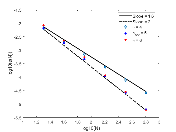
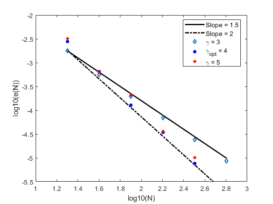
Figure 1: Temporal accuracy of (3.1) for $\alpha=0.8,\sigma=0.4$ and $\alpha=0.5,\sigma=0.5$.

We test the time accuracy with the $L^{2}$ norm errors $e(N):=\max_{1\leq n\leq N}\big{\|}\Phi^{n}-\phi^{n}\big{\|}$. By setting different grading parameters $\gamma>1$, the numerical results in Figure 1 are computed for $\sigma=0.4,\,\alpha=0.8$ and $\sigma=\alpha=0.5$, respectively. As observed, the variable-step L2-1_σ scheme (3.1) is of order $O(\tau^{\gamma\sigma})$ if the grading parameter $\gamma<\gamma_{\text{opt}}=2/\alpha$, while the optimal time accuracy $O(\tau^{2})$ can be attained when the grading parameter $\gamma\geq\gamma_{\text{opt}}$.

5.2 Simulation of coarsening dynamics

Example 2.

The coarsening dynamics of the TFAC model is examined with $\epsilon=0.05$. The initial condition is generated as $\Phi_{0}(\mathbf{x})=\mathrm{rand}(\mathbf{x})$, where $\mathrm{rand}(\mathbf{x})$ is uniformly distributed random number varying from $-0.001$ to 0.001 at each grid point.

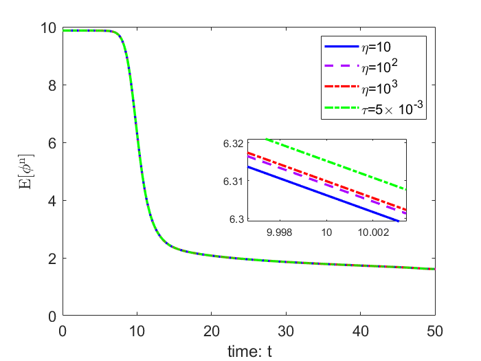
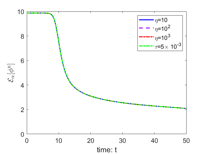
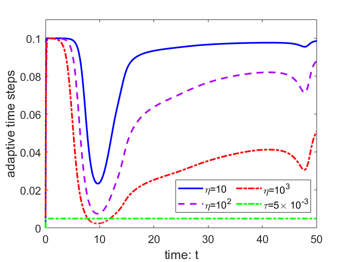
Figure 2: Energy curves from adaptive strategy for different parameters $\eta$.

We use a $128^{2}$ grid to discretize the domain $(0,2\pi)^{2}$. The graded mesh $t_{k}=T_{0}(k/N_{0})^{\gamma}$ with the settings $\gamma=3,N_{0}=30$ and $T_{0}=0.01$ are always applied in the initial part $[0,T_{0}]$, cf. [10]. In order to improve the computational efficiency of long-time numerical simulation and accurately capture the rapid changes of energy and numerical solution, we adopt the following adaptive time-stepping strategy to adjust the step size by the change rate of the solution [30, 9]

$$\tau_{ada}=\max\big{\{}\tau_{\min},\tau_{\max}/\varPi(\phi,\eta)\big{\}}\quad\text{so that}\quad\tau_{n+1}=\max\{\tau_{ada},r_{\star}\tau_{n}\},$$

where $\tau_{\max}$ and $\tau_{\min}$ are the predetermined maximum and minimum size of time-steps, and $\varPi(\phi,\eta):=\sqrt{1+\eta\big{\|}\partial_{\tau}\phi^{n-\frac{1}{2}}\big{\|}^{2}}$ with a user parameter $\eta$ to be determined. We take $\tau_{\max}=10^{-1}$, $\tau_{\min}=10^{-3}$, $T_{0}=0.01$, $\gamma=3$ and consider three different parameters $\eta=10,10^{2}$ and $10^{3}$ to determine a suitable parameter $\eta$ where the fractional index $\alpha=0.7$, T=50 and the reference solution is computed by using the uniform time step $\tau=5\times 10^{-3}$. As seen in Figure 2, the value of parameter $\eta$ evidently influences on the adaptive sizes of time steps. The time-steps have the smallest fluctuation if $\eta=10^{3}$ and the energy curve is closer to the reference curve.

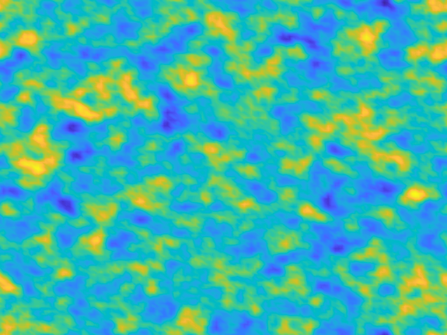
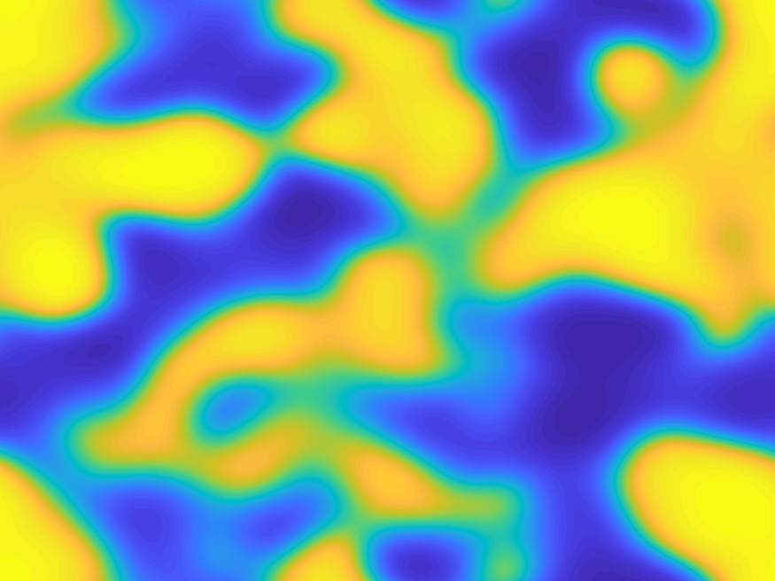
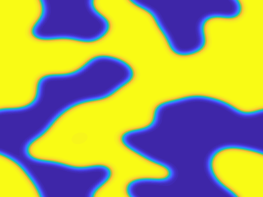
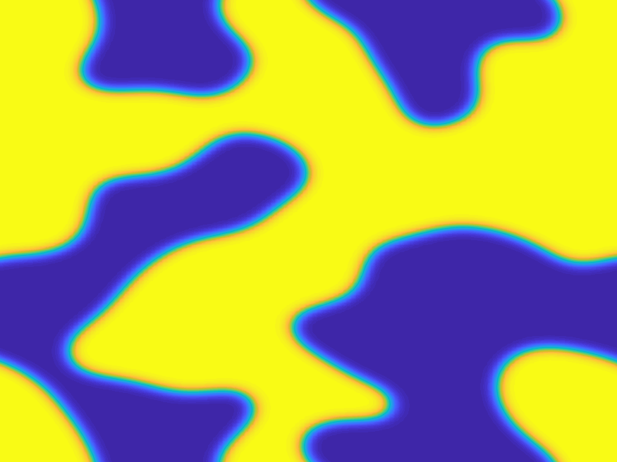
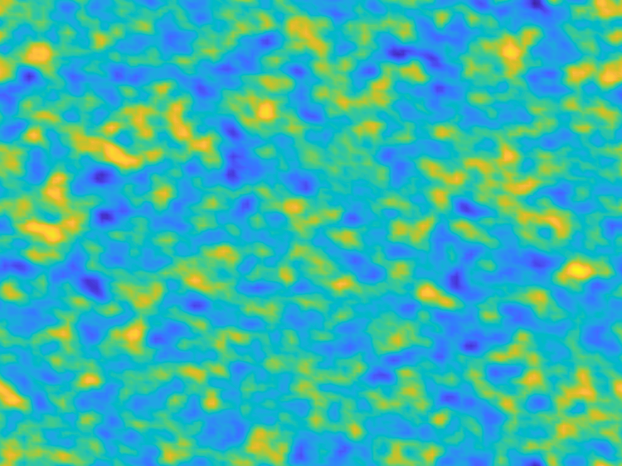
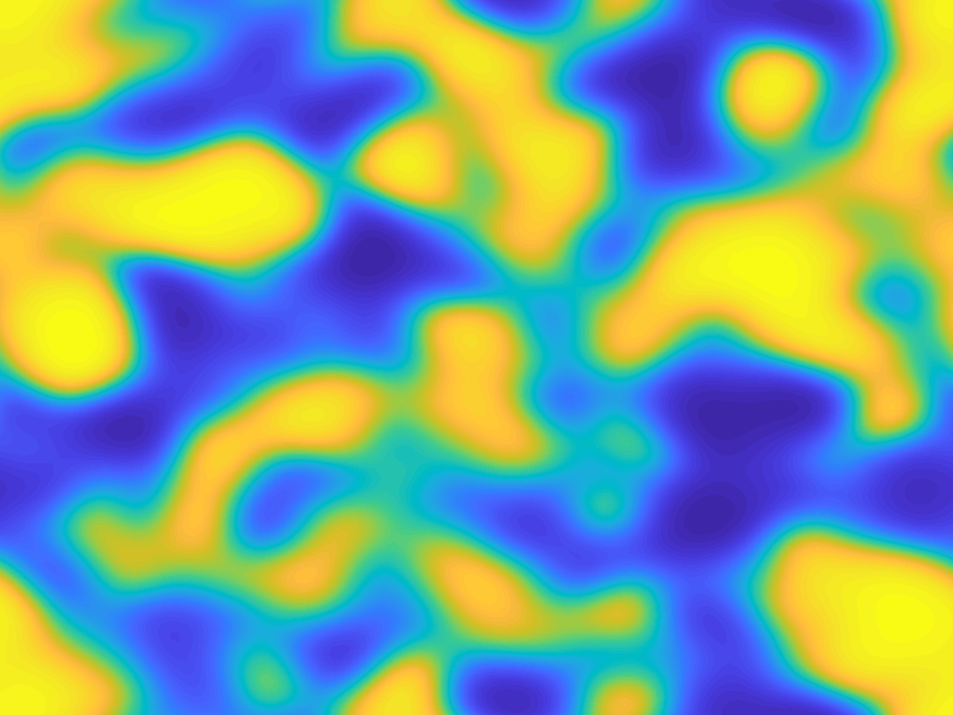
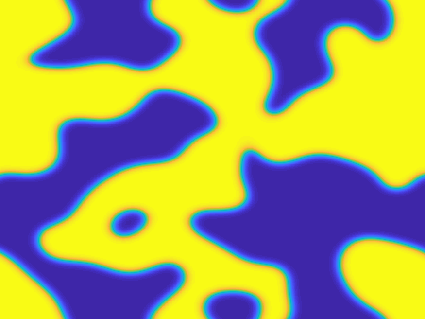
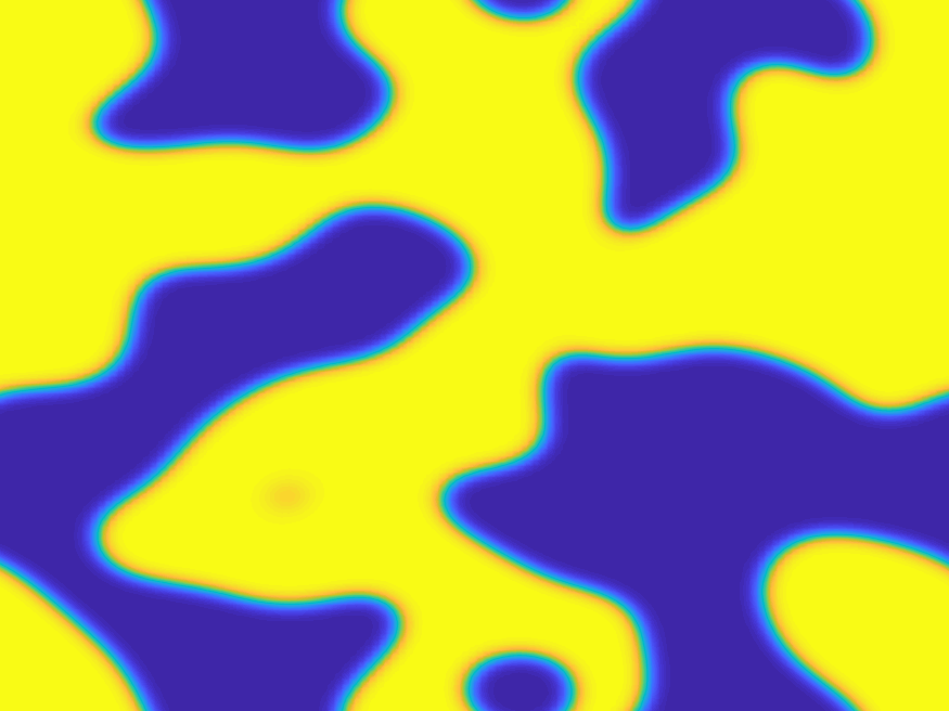
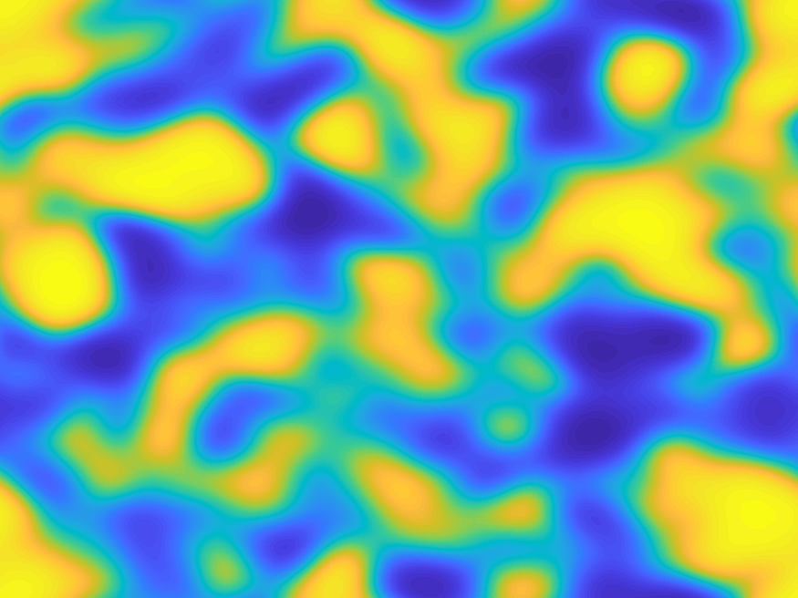
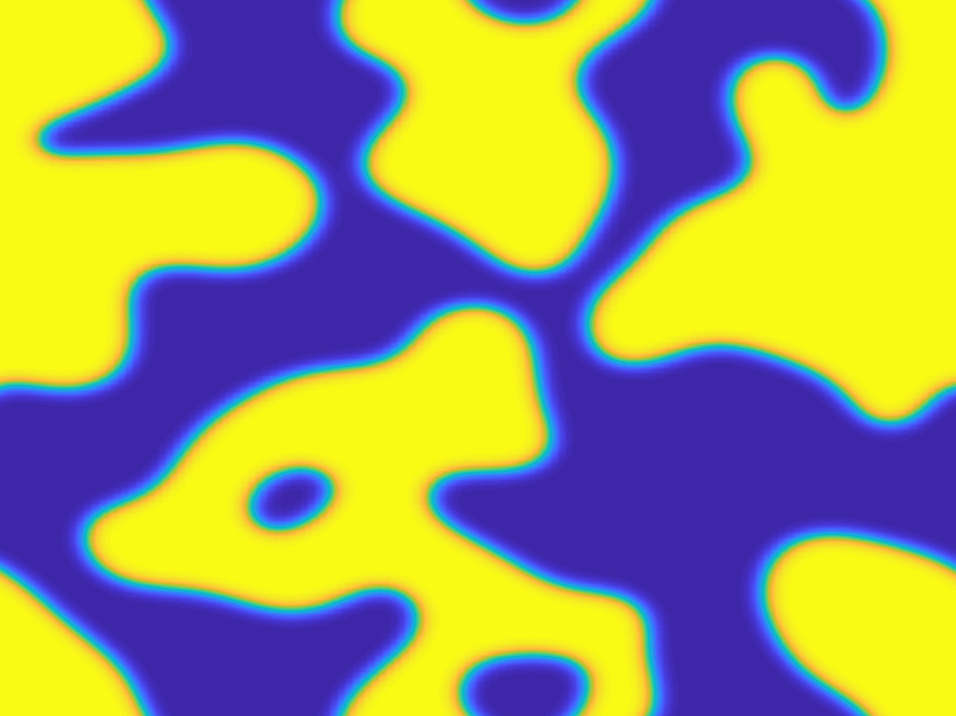
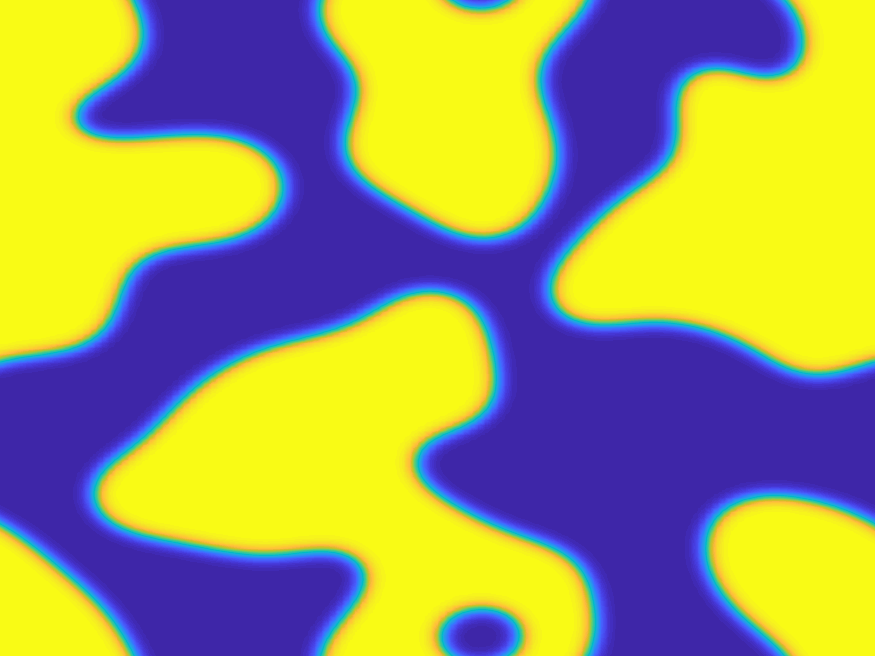
Figure 3: Profiles of coarsening dynamics at $t=1,10,30,50$ (from left to right) for three different fractional orders $\alpha=0.4,0.7,0.9$ (from top to bottom).

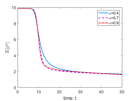
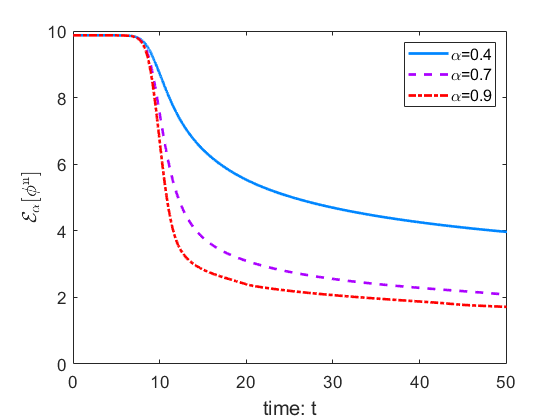
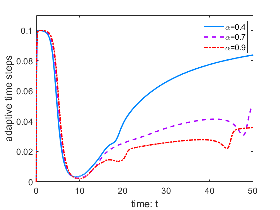
Figure 4: $E(t)$, $\mathcal{E}_{\alpha}(t)$ and adaptive time steps for the fractional orders $\alpha=0.4,0.7,0.9$.

Next, by taking $\tau_{\max}=10^{-1}$, $\tau_{\min}=10^{-3}$ and the parameter $\eta=10^{3}$ in the adaptive time-stepping strategy, the profiles of coarsening dynamics with different fractional orders $\alpha=0.4,0.7$ and 0.9 for the TFAC model are shown in Figure 3. Snapshots are taken at time $t=1,10,30$ and 50, respectively. We observe that the coarsening rates of TFAC model are dependent on the fractional order and the time period. The calculated energies using the adaptive time steps for the coarsening dynamics are depicted in Figure 4, which shows that the original energy and the modified energy for TFAC model with $\alpha=0.4,0.7$ and 0.9 are both decreasing respect to time. And the adaptive time steps strategy is successful in adjusting the time steps.

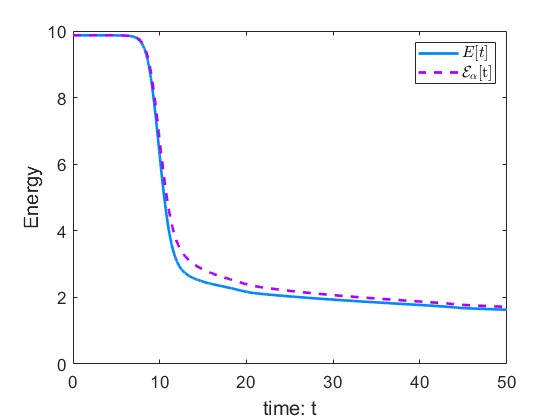
Figure 5: Comparison of $E(t)$ and $\mathcal{E}_{\alpha}(t)$ for $\alpha=0.9,0.95,0.97$ (from left to right).

Figure 5 compares the curves of $E(t)$ and $\mathcal{E}_{\alpha}(t)$ for different fractional orders $\alpha=0.9,0.95,0.97$ to illustrate the asymptotic compatibility of the new discrete energy. As expected, the closer the time fractional index is to 1, the closer the modified energy $\mathcal{E}_{\alpha}(t)$ is to the original energy $E(t)$.

Funding

This work is supported by NSF of China under Grant Number 12071216.

Data Availibility Statement

All data generated or analysed during this study are included in this published article.

Declarations

The authors declare that they have no conflict of interest.

Compliance with Ethical Standards

This article does not contain any studies involving animals performed by any of the authors.

References

- [1] A. A. Alikhanov. A new difference scheme for the time fractional diffusion equation. J. Comput. Phys., 280:424-438, 2015.
- [2] S. Allen and J. Cahn. A microscopic theory for antiphase boundary motion and its application to antiphase domain coarsening. Acta Metall., 27:1085-1095, 1979.
- [3] Q. Du, J. Yang and Z. Zhou. Time-fractional Allen-Cahn equations: Analysis and numerical methods. J. Sci. Comput., 85:11, 2020.
- [4] X. Feng and A. Prohl. Numerical analysis of the Allen-Cahn equation and approximation for mean curvature flows. Numer. Math., 94:33-65, 2003.
- [5] D. Hou and C. Xu. Highly efficient and energy dissipative schemes for time fractional Allen-Cahn equation. SIAM J. Sci. Comput., 43(5):A3305-A3327,2021.
- [6] D. Hou, H. Zhu and C. Xu. Highly efficient schemes for time-fractional Allen–Cahn equation using extended SAV approach. Numer. Algorithms, 88:1077-1108, 2021.
- [7] D. Hou and C. Xu. A second order energy dissipative scheme for time fractional gradient flows using SAV approach. J. Sci. Comput., 90(1):1-22, 2022.
- [8] T. Hou, T. Tang and J. Yang. Numerical analysis of fully discretized Crank-Nicolson scheme for fractional-in-space Allen-Cahn equations. J. Sci. Comput., 72(3):1214-1231, 2017.
- [9] J. Huang, C. Yang and Y. Wei. Parallel energy-stable solver for a coupled Allen-Cahn and Cahn-Hilliard system. SIAM J. Sci. Comput., 42:C294-C312, 2020.
- [10] B. Ji, H.-L. Liao and L. Zhang. Simple maximum-principle preserving time-stepping methods for time-fractional Allen-Cahn equation. Adv. Comput. Math., 46:37, 2020.
- [11] B. Ji, H.-L. Liao, Y. Gong, and L. Zhang. Adaptive second-order Crank-Nicolson timestepping schemes for time fractional molecular beam epitaxial growth models. SIAM J. Sci. Comput., 42:B738–B760, 2020.
- [12] B. Ji, X. Zhu and H-L. Liao. Energy stability of variable-step L1-type schemes for time-fractional Cahn-Hilliard model. arXiv:2201.00920, 2022.
- [13] S. Jiang, J. Zhang, Z. Qian and Z. Zhang. Fast evaluation of the Caputo fractional derivative and its applications to fractional diffusion equations. Commun. Comput. Phys., 21:650-678, 2017.
- [14] S. Karaa, Positivity of discrete time-fractional operators with applications to phase-field equations, SIAM J. Numer. Anal., 59:2040-2053, 2021.
- [15] N. Kopteva, Error analysis for time-fractional semilinear parabolic equations using upper and lower solutions, SIAM J. Numer. Anal., 58:2212-2234, 2020.
- [16] N. Kopteva and X. Meng, Error analysis for a fractional-derivative parabolic problem on quasi-graded meshes using barrier functions, SIAM J. Numer. Anal., 58:1217-1238, 2020.
- [17] Z. Li, H. Wang and D. Yang, A space-time fractional phase-field model with tunable sharpness and decay behavior and its efficient numerical simulation, J. Comput. Phys., 347: 20-38, 2017.
- [18] H.-L. Liao, N. Liu and X. Zhao. Asymptotically compatible energy of variable-step fractional BDF2 formula for time-fractional Cahn-Hilliard model. arXiv: 2210.12514v1, 2022.
- [19] H.-L. Liao, W. McLean and J. Zhang. A discrete Grönwall inequality with application to numerical schemes for subdiffusion problems. SIAM J. Numer. Anal., 57:218-237, 2019.
- [20] H.-L. Liao, W. McLean and J. Zhang. A second-order scheme with nonuniform time steps for a linear reaction-subdiffusion problem. Commun. Comput. Phys., 30(2):567-601, 2021.
- [21] H.-L. Liao, T. Tang and T. Zhou. A second-order and nonuniform time-stepping maximum-principle preserving scheme for time-fractional Allen-Cahn equations. J. Comput. Phys., 414:109473, 2020.
- [22] H.-L. Liao, T. Tang and T. Zhou. An energy stable and maximum bound preserving scheme with variable time steps for time fractional Allen-Cahn equation. SIAM J. Sci. Comput., 43(5):A3503-A3526, 2021.
- [23] H.-L. Liao, X. Zhu and J. Wang. An adaptive L1 time-stepping scheme preserving a compatible energy law for the time-fractional Allen-Cahn equation. Numer. Math. Theor. Meth. Appl., 15(4):1128-1146, 2022.
- [24] H. Liu, A. Cheng, H. Wang and J. Zhao. Time-fractional Allen-Cahn and Cahn-Hilliard phase-field models and their numerical investigation. Comput. Math. Appl., 76:1876-1892, 2018.
- [25] C. Quan, T. Tang, B. Wang and J. Yang. A decreasing upper bound of energy for time-fractional phase-field equations. arXiv:2202.12192v1, 2022.
- [26] C. Quan, T. Tang and J. Yang. How to define dissipation-preserving energy for time-fractional phase-field equations. CSIAM-AM, 1:478-490, 2020.
- [27] C. Quan and X. Wu. On stability and convergence of L2-1σ method on general nonuniform meshes for subdiffusion equation. arXiv:2208.01384v1, 2022.
- [28] C. Quan and X. Wu, H1-stability of an L2 method on general nonuniform meshes for subdiffusion equation, arXiv:2205.06060v1, 2022.
- [29] T. Tang, H. Yu and T. Zhou. On energy dissipation theory and numerical stability for time-fractional phase field equations. SIAM J. Sci. Comput., 41:A3757-A3778, 2019.
- [30] Z. Zhang and Z. Qiao. An adaptive time-stepping strategy for the Cahn-Hilliard equation. Commun. Comput. Phys., 11:1261-1278, 2012.
- [31] J. Zhao, L. Chen and H. Wang, On power law scaling dynamics for time-fractional phase field models during coarsening. Commun. Nonlinear Sci., 70:257-270, 2019.