Robust Multi-Model Subset Selection

Abstract

Modern datasets in biology and chemistry are often characterized by the presence of a large number of variables and outlying samples due to measurement errors or rare biological and chemical profiles. To handle the characteristics of such datasets we introduce a method to learn a robust ensemble comprised of a small number of sparse, diverse and robust models, the first of its kind in the literature. The degree to which the models are sparse, diverse and resistant to data contamination is driven directly by the data based on a cross-validation criterion. We establish the finite-sample breakdown of the ensembles and the models that comprise them, and we develop a tailored computing algorithm to learn the ensembles by leveraging recent developments in $\ell_{0}$ optimization. Our extensive numerical experiments on synthetic and artificially contaminated real datasets from bioinformatics and cheminformatics demonstrate the competitive advantage of our method over state-of-the-art sparse and robust methods. We also demonstrate the applicability of our proposal on a cardiac allograft vasculopathy dataset.

Keywords: Robust methods; High-dimensional data; Ensemble methods; Multi-model optimization.

1 Introduction

With the acceleration of technological advances in data collecting and storing technologies in many fields of science and engineering, there is an ever-increasing need for new statistical methods that can handle complex biological and chemical data. The type of biological and chemical data collected by these types of technologies are typically characterized by a large number of measurements (variables) $p$ combined with a limited number of samples $n$, and also by potential data contamination due to measurement errors or rare sample profiles. In the statistical literature, data characterized by a large number of variables relative to the number of samples (i.e. $p\gg n$) is known as high-dimensional data. Such data pose a significant statistical challenge as it is typically the case that only a subset of the variables are needed to obtain a reliable statistical model to predict some outcome of interest. Parsimonious models are also more interpretable and may help to understand the biological or chemical process underlying the data. For example, high-throughput DNA or RNA sequencing technologies can collect the expression levels of thousands of genes, and it is typically preferred to obtain a model that only uses a small subset of genes to accurately predict the biological outcome of interest. In a cheminformatics application where the spectrum of a chemical compound is collected by advanced particle-beam technologies, it may be desired to obtain a model that only uses a small subset of the frequency measurements to accurately predict the concentration of the compound. Data contamination is also a common feature of data collected by laboratory instruments since they are prone to all kinds of measurement errors. To make matters more complication the atypical (or outlying) samples in the data may not be due to measurement errors, instead they may be samples with rare genetic, molecular or chemical profiles.

To address the issue of high-dimensionality, many sparse methods have been proposed in the literature. These methods typically yield a single interpretable model that only uses a subset of the variables. The empirical performance and theoretical properties of sparse methods have been studied extensively, see e.g. Hastie et al. (2019) for a modern treatment. Another topic that has received considerable attention in the literature is statistical robustness, which addresses the issue of data contamination. Robust statistical procedures typically replace traditional loss functions by robust loss functions that downweigh the effect of contaminated samples on model parameters, see e.g. Maronna et al. (2019) for a modern theoretical and computational treatment of robust statistics. In recent years there have been many proposals that combine sparse and robust methods to obtain a single interpretable model that is resistant to outliers. The models generated by these sparse and robust methods have been successful in a variety of applications using high-dimensional biological and chemical data, see e.g. Alfons et al. (2013); Smucler and Yohai (2017); Cohen Freue et al. (2019).

Ensemble methods, which generate and aggregate multiple diverse models, are an alternative to sparse methods when dealing with high-dimensional data and often outperform sparse methods in high-dimensional prediction tasks. Traditionally, ensemble methods rely on randomization or some form of heuristics to generate diverse models, and are thus considered “blackbox” methods. Prominent ensemble methods relying on randomization include random forests (RF) (Breiman, 2001) and random generalized linear models (RGLM) (Song et al., 2013), while prominent ensemble methods relying on heuristics include gradient boosting (Friedman, 2001) and all its variations (see e.g. Bühlmann and Yu, 2003; Schapire and Freund, 2012; Chen and Guestrin, 2016). These types of ensemble methods generate a large number of uninterpretable and inaccurate models that are only useful when they are pooled together. More recently, Christidis et al. (2020) and Christidis et al. (2023) proposed methods that generate ensembles comprised of a small number of sparse and diverse models learned directly from the data without any form of randomization or heuristics. Each of the models in these ensembles have a high prediction accuracy similar to sparse methods, and the ensembling of a small number of these accurate and interpretable models was shown to outperform state-of-the-art blackbox ensemble methods on synthetic as well as complex biological and chemical data. However, both the ensembles and the individual models that comprise them are not robust and are thus very sensitive to outliers.

In this article we introduce robust multi-model subset selection (RMSS), a method that robustifies the proposal of Christidis et al. (2023) in order to learn an ensemble comprised of a small number of sparse, robust and diverse models in a regression setting. In our proposal the degree to which the models are sparse, robust and diverse is driven directly by the data. We establish the finite-sample breakdown point of these robust ensembles and the individual models that comprise them. We develop a tailored computational algorithm with its convergence properties to fit the models. RMSS is shown to outperform state-of-the-art sparse and robust methods in an extensive simulation study and when applied to artificially contaminated biological and chemical data. We also demonstrate the applicability of RMSS on a cardiac allograft vasculopathy dataset. To the best of our knowledge this is the first robust ensemble proposed in the statistical literature, and also the first proposal that combines the appeal of data-driven sparsity, robustness and ensemble model diversity into a single method.

The remainder of this article is organized as follows. In Section 2, we provide a brief overview of the state-of-the-art for sparse, robust and ensemble methods. In Section 3 we formally introduce RMSS and discuss some of its special cases. In Section 4 we establish the finite-sample breakdown point of RMSS ensembles and the individual models that comprise them. In Section 5 we provide a computational algorithm to generate RMSS ensembles and establish some of its convergence properties. In Section 6 we benchmark RMSS against state-of-the-art sparse and robust methods in a large simulation study. In Section 7 we apply RMSS on artificially contaminated datasets from bioinformatics and cheminformatics, and in Section 8 in a cardiac allograft vasculopathy data application. Summarizing remarks and a discussion for potential future works are given in Section 9.

2 Literature Review

We consider a regression setting where the relationship between a response vector $\mathbf{y}=(y_{1},\dots,y_{n})^{T}\in\mathbb{R}^{n}$ and a design matrix $\mathbf{X}\in\mathbb{R}^{n\times p}$ containing $n$ observations $\mathbf{x}_{i}=(x_{i1},\dots,x_{ip})^{T}\ (i=1,\dots,n)$ for $p$ predictor variables can be modelled by the linear model

$$y_{i}=\mathbf{x}_{i}^{T}\boldsymbol{\beta}_{0}+\sigma\epsilon_{i},\quad 1\leq i\leq n,$$ (1)

where $\boldsymbol{\beta}_{0}\in\mathbb{R}^{p}$ and the elements of the noise vector $\boldsymbol{\epsilon}=(\epsilon_{1},\dots,\epsilon_{n})^{T}\in\mathbb{R}^{n}$ are independent and identically distributed with mean zero and variance one. We focus our attention on the high-dimensional setting ($p\gg n$) where the underlying model is sparse, i.e. the number of nonzero elements of the true coefficient vector $\left\lVert\boldsymbol{\beta}_{0}\right\rVert_{0}\ll p$. We assume that a (strict) subset of the samples may be contaminated, and that the relationship between the predictors and the response variable of the contaminated samples may deviate from the linear model (1). Due to the potential contamination of the data, we assume that the response $\mathbf{y}$ and the columns of the design matrix $\mathbf{X}$ are centered and scaled using their medians and median absolute deviations (from their medians), respectively. For simplicity, we omit the intercept term from the true regression model.

2.1 Sparse Methods

Sparse methods were introduced in the literature to generate interpretable models where only a small subset of the predictor variables are used, particularly when $p$ may be very large. Beyond the appeal of model interpretability and parsimony, sparse methods also have favorable properties in terms of parameters estimation and prediction when the true underlying model is sparse (see e.g. Bühlmann and Van De Geer, 2011).

The Best Subset Selection (BSS) estimator proposed by Garside (1965) was one of the first sparse estimator proposed in the literature, and is given by the solution to the non-convex (and non-differentiable) objective function

$$\min_{\boldsymbol{\beta}\in\mathbb{R}^{p}}\left\lVert\mathbf{y}-\mathbf{X}\boldsymbol{\beta}\right\rVert_{2}^{2}\quad\text{subject to}\quad\left\lVert\boldsymbol{\beta}\right\rVert_{0}\leq t,$$ (2)

where $t\leq\min(n-1,p)$ is the number of nonzero coefficients allowed in the coefficient vector $\boldsymbol{\beta}$ and may be chosen by a model selection criterion (see e.g. Mallows, 1973; Akaike, 1974) or by cross-validation (CV).

Since the BSS optimization problem (2) is an NP-hard problem (Welch, 1982), many sparse regularization methods in the form of convex relaxations of (2) were proposed in the literature to avoid the computational infeasibility of BSS. Prominent examples include the least absolute shrinkage and selection operator (Lasso) (Tibshirani, 1996) and the elastic net (EN) (Zou and Hastie, 2005), which solve convex optimization problems of the form

$$\min_{\boldsymbol{\beta}\in\mathbb{R}^{p}}\left\lVert\mathbf{y}-\mathbf{X}\boldsymbol{\beta}\right\rVert_{2}^{2}+\lambda P\left(\boldsymbol{\beta}\right),$$ (3)

where $P(\boldsymbol{\beta})$ is a convex penalty function in terms of the coefficient vector $\boldsymbol{\beta}$ and $\lambda\in\mathbb{R}^{+}$ is typically chosen by CV. The EN penalty is given by

$$P(\boldsymbol{\beta})=\alpha\left\lVert\boldsymbol{\beta}\right\rVert_{1}+\frac{1-\alpha}{2}\left\lVert\boldsymbol{\beta}\right\rVert_{2}^{2},$$ (4)

where the case $\alpha=1$ corresponds to the Lasso. Efficient convex solvers and their software implementations have been developed for sparse regularization methods (see e.g. Friedman et al., 2007; Friedman et al., 2010). Two-step regularization methods have also been proposed to improve the theoretical and variable selection properties of one-step regularization methods (see e.g. Zou, 2006; Meinshausen, 2007).

Although convex relaxations have much lower computational cost, BSS enjoys better estimation and variable selection properties compared to sparse regularization methods (see e.g. Bunea et al., 2007; Van De Geer and Bühlmann, 2009; Shen et al., 2013), and often outperforms regularization methods in high-dimensional prediction tasks (see e.g. Hazimeh and Mazumder, 2020; Hastie et al., 2020). Recently there has been a revival of BSS in the literature and the appearance of innovative work on fast and scalable algorithms to generate solutions to the BSS problem (2). In particular Bertsimas et al. (2016) paved the way for such research by developing computing algorithms for $\ell_{0}$ optimization with local convergence guarantees, and showing that the BSS problem (2) can be cast a a mixed integer optimization (MIO) problem. Recent extensions of this work include Bertsimas and Van Parys (2020), Hazimeh and Mazumder (2020), Takano and Miyashiro (2020) and Kenney et al. (2021). In another line of research for BSS, Zhu et al. (2020) developed a tailored “splicing” algorithm with polynomial computational complexity that can recover the optimal global solution under relatively mild assumptions.

2.2 Robust Methods

A common feature of many modern datasets is the presence of outliers. Within the rich literature on robust statistics, M-regression (Huber, 1964) is one of the earliest and most popular method for fitting regression models on contaminated data. M-estimators of regression are defined by solutions to optimization problems of the form

$$\min_{\boldsymbol{\beta}\in\mathbb{R}^{p}}\frac{1}{n}\sum_{i=1}^{n}\rho\left(\frac{y_{i}-\sum_{j=1}^{p}\beta_{j}x_{ij}}{\hat{\sigma}}\right),$$ (5)

where $\rho$ is a bounded loss function, for e.g. Tukey’s Bisquare loss function $\rho(t)=\min\{1,1-(1-(t/c)^{2})^{3}\}$, and $\hat{\sigma}$ is a pre-computed robust residual scale estimator. Subsequently, Rousseeuw and Yohai (1984) introduced S-regression estimators, defined by solutions to problems of the form

$$\min_{\boldsymbol{\beta}\in\mathbb{R}^{p}}\sigma^{2}\left(\boldsymbol{\beta}\right)$$ (6)

where $\sigma^{2}(\boldsymbol{\beta})$ is a robust M-estimate of scale given implicitly by the solution of

$$\frac{1}{n}\sum_{i=1}^{n}\rho\left(\frac{y_{i}-\sum_{j=1}^{p}\beta_{j}x_{ij}}{\sigma^{2}\left(\boldsymbol{\beta}\right)}\right)=\delta,\quad\delta\in(0,1).$$ (7)

Both M-estimators and S-estimators of regression can sustain up to 50% of contaminated samples and share similar asymptotic properties. In a parallel line of research, Yohai (1987) introduced MM-estimators of regression, M-estimators of regression for which the residual scale $\hat{\sigma}$ is given by the solution of S-estimators of regression $\hat{\sigma}(\boldsymbol{\hat{\beta}})$ in (6). MM-estimators of regression can also sustain up to 50% of contaminated samples, but unlike its predecessors they maintain a high efficiency under normal errors.

Another popular robust regression tool is the least trimmed squares (LTS) estimator introduced by Rousseeuw (1984). Let $I=\{1,\dots,n\}$ and denote $|\cdot|$ the cardinality operator. The LTS estimator is defined by the optimization problem

$$\min_{\boldsymbol{\beta}\in\mathbb{R}^{p}}\sum_{i\in{I}}\left(y_{i}-\mathbf{x}_{i}^{T}\boldsymbol{\beta}\right)^{2}\quad\text{subject to}\quad|I|\geq h,$$ (8)

where $h\leq\lfloor n/2\rfloor$, i.e. the smallest sum of squares under the restriction that no more than $n-h$ samples are “trimmed” from the sum. A thorough theoretical treatment of LTS estimators is available in Rousseeuw and Leroy (2005).

Robust methods often pose significant computational challenges since they typically involve non-convex optimization problems. In the case of objective functions with a bounded loss function such as Tukey’s Bisquare, a common strategy is to obtain many initial estimators by fitting the non-robust regression model on random subsets of the data with the aim to obtain clean subsets without outliers (see e.g. Salibian-Barrera and Yohai, 2006; Koller and Stahel, 2017). As an alternative, Peña and Yohai (1999) and Maronna (2011) introduced methods that flag potentially outlying samples by measuring their effect on the estimated model parameters, and then take as initial estimator the non-robust regression model on the clean data. In LTS where the objective function is binary (samples may be included or excluded), many heuristics have been developed in the literature to obtain fast approximations to the global optimal solution (see e.g. Hawkins, 1994; Atkinson and Cheng, 1999; Giloni and Padberg, 2002; Li, 2005; Rousseeuw and Van Driessen, 2006; Ding and Xu, 2014).

2.3 Sparse and Robust Methods

To handle datasets that are high-dimensional and may also contain outliers, sparse and robust methods have been introduced in the literature over the last two decades. In the proposals of Khan et al. (2007a) and Khan et al. (2007b), the authors showed that the stepwise and least angle regression (LARS) (Efron et al., 2004) algorithms can be recast by only looking at the pairwise correlations between variables. The authors proposed to compute robust pairwise correlations based on bivariate winsorization of the data, apply the stepwise or LARS algorithm to select variables, and finally fit MM-regression models on the reduced subset of variables.

Subsequently, Alfons et al. (2013) introduced sparse LTS in the literature where the objective function is given by

$$\min_{\boldsymbol{\beta}\in\mathbb{R}^{p}}\sum_{i\in{I}}\left(y_{i}-\mathbf{x}_{i}^{T}\boldsymbol{\beta}\right)^{2}+\lambda P(\boldsymbol{\beta})\quad\text{subject to}\quad|I|\geq h,$$ (9)

and $P(\boldsymbol{\beta})$ is the EN penalty defined in (4). Smucler and Yohai (2017) combined MM-regression with the Lasso penalty, and Cohen Freue et al. (2019) introduced the penalized elastic net S-estimator (PENSE) and developed its theoretical properties and an efficient computing algorithm. PENSE is defined by the optimization problem

$$\min_{\boldsymbol{\beta}\in\mathbb{R}^{p}}\sigma^{2}\left(\boldsymbol{\beta}\right)+\lambda P\left(\boldsymbol{\beta}\right),$$ (10)

where $P(\boldsymbol{\beta})$ is the EN penalty (4) and $\sigma^{2}(\boldsymbol{\beta})$ is the robust M-estimate of scale implicitly given by (7). Kepplinger (2023) extended this work and developed a two-step adaptive PENSE method. In a similar line of research Yi and Huang (2017) developed efficient algorithms to fit robust regression models using the Huber Huber (1964) with the EN penalty.

Thompson (2022) introduced robust best subset selection (RBSS) by combining the LTS loss with the $\ell_{0}$ penalty for the vector of coefficients,

$$\min_{\boldsymbol{\beta}\in\mathbb{R}^{p}}\sum_{i\in{I}}\left(y_{i}-\mathbf{x}_{i}^{T}\boldsymbol{\beta}\right)^{2}\quad\text{subject to}\quad\begin{cases}\left\lVert\boldsymbol{\beta}\right\rVert_{0}\leq t,\\ |{I}|\geq h.\end{cases}$$ (11)

Thompson (2022) established the finite-sample breakdown point of RBSS, and developed a computing algorithm with tailored heuristics to refine the solution in search of the optimal global solution. This work forms part of the basis for our proposal in this article.

2.4 Ensemble Methods

The competitive advantage of ensemble methods over single-model methods can be seen through the decomposition of the mean squared prediction error (MSPE) of regression ensembles. Let $\hat{f}_{g}(\mathbf{x})$, $1\leq g\leq G$, be the regression functions that comprise an ensemble, and let $\bar{f}(\mathbf{x})=\sum_{g=1}^{G}\hat{f}_{g}(\mathbf{x})/G$ be the simple average of the $G$ regression functions. Ueda and Nakano (1996) showed that the MSPE of such a regression ensemble can be decomposed as

$$\text{MSPE}\left[\bar{f}\right]=\text{Bias}\left[\bar{f}\right]^{2}+\text{Var}\left[\bar{f}\right]+\sigma^{2},$$ (12)

with

$$\text{Bias}\left[\bar{f}\right]=\overline{\text{Bias}}\quad\text{and}\quad\text{Var}\left[\bar{f}\right]=\frac{1}{G}\,\overline{\text{Var}}+\frac{G-1}{G}\,\overline{\text{Cov}},$$ (13)

where $\overline{\text{Bias}}$, $\overline{\text{Var}}$ and $\overline{\text{Cov}}$ are the average biases, variances and pairwise covariances of the $G$ regression functions in the ensemble, and $\sigma^{2}$ is the irreducible error. If an ensemble is comprised of a large number of models, then by (13) the variance term of the ensemble is largely determined by how correlated its individual models are.

Until recently, most ensemble methods relied on a large number of models (typically $G>100$) and weak decorrelated models to lower the MSPE of ensembles. In the well known RF method of Breiman (2001), decorrelation of the individual trees is achieved by random sampling of the data (i.e. bagging, Breiman, 1996a) and random sampling of the predictors (i.e. the random predictor subspace method, Ho, 1998). A similar approach is used in the RGLM method of Song et al. (2013) to generate a large number of diverse linear models. Another method to generate a large number of diverse models is through gradient boosting, i.e. the sequential refitting of residuals (see e.g. Chen and Guestrin, 2016). Beyond the weak predictive accuracy of the individual models in such ensembles, they are also not interpretable. The selection of predictor variables is unreliable if randomization is used, and in the case of gradient boosting the models are fit on residuals rather than the original data.

To generate ensembles of sparse, accurate and diverse models, Christidis et al. (2020) and Christidis et al. (2023) relied on the principle of the multiplicity of good models (see e.g. McCullagh and Nelder, 1989; Mountain and Hsiao, 1989). In particular when there are a lot of predictor variables, there may be multiple models comprised of different subsets of predictors that may able to achieve a good prediction accuracy. Christidis et al. (2020) search for such models by solving the optimization problem

$$\mathcal{J}\left(\mathbf{y},\mathbf{X},\boldsymbol{\beta}^{1},\dots,\boldsymbol{\beta}^{G}\right)=\sum_{g=1}^{G}\left\{\frac{1}{2n}\left\lVert\mathbf{y}-\mathbf{X}\boldsymbol{\beta}^{g}\right\rVert_{2}^{2}+\lambda_{s}P_{d}\left(\boldsymbol{\beta}^{g}\right)+\frac{\lambda_{d}}{2}\sum_{g\neq h}^{G}P_{d}\left(\boldsymbol{\beta}^{h},\boldsymbol{\beta}^{g}\right)\right\}$$ (14)

where $P_{s}$ is a sparsity penalty function (e.g. the EN), $P_{d}$ is a diversity penalty that encourages models to use different subset of predictors and $\boldsymbol{\beta}^{g}\in\mathbb{R}^{p}$ is the vector of coefficients for model $g$, $1\leq g\leq G$. To alleviate using the multi-convex relaxation in (14) and control the degrees of sparsity and diversity directly, Christidis et al. (2023) introduced multi-model subset selection (MSS) as a generalization of BSS in (2). Denote the matrix of coefficients for $G$ models in an ensemble by

$$\boldsymbol{\beta}_{1:G}=\begin{pmatrix}\beta_{1}^{1}&\beta_{1}^{2}&\dots&\beta_{1}^{G}\\ \beta_{2}^{1}&\beta_{2}^{2}&\dots&\beta_{2}^{G}\\ \vdots&\vdots&\ddots&\vdots\\ \beta_{p}^{1}&\beta_{p}^{2}&\dots&\beta_{p}^{G}\end{pmatrix},$$ (15)

where $\boldsymbol{\beta}_{1:G}\in\mathbb{R}^{p\times G}$ and $\beta_{j}^{g}$ is the coefficient for predictor $j$ in model $g$, $1\leq g\leq G$. Again denote $\boldsymbol{\beta}^{g}=(\beta_{1}^{g},\beta_{2}^{g},\dots,\beta_{p}^{g})^{T}\in\mathbb{R}^{p}$ the coefficients of model $g$, and also let $\boldsymbol{\beta}_{j\cdot}=(\beta_{j}^{1},\beta_{j}^{2},\dots,\beta_{j}^{G})^{T}\in\mathbb{R}^{G}$ be the coefficients of predictor $j$ across the $G$ models. MSS searches for $G\geq 2$ accurate models by solving the optimization problem

$$\min_{\boldsymbol{\beta}^{1},\dots,\,\boldsymbol{\beta}^{G}\in\mathbb{R}^{p}}\sum_{g=1}^{G}\|\mathbf{y}-\mathbf{X}\boldsymbol{\beta}^{g}\|_{2}^{2}\quad\text{subject to}\quad\begin{cases}\left\lVert\boldsymbol{\beta}^{g}\right\rVert_{0}\leq t,\,&1\leq g\leq G,\\ \left\lVert\boldsymbol{\beta}_{j\cdot}\right\rVert_{0}\leq u,\,&1\leq j\leq p,\end{cases}$$ (16)

where the parameter $t\leq\min(n-1,p)$ restricts the $\ell_{0}$-norm of the columns of $\boldsymbol{\beta}_{1:G}$ and thus controls the degree of sparsity of each model in the ensemble. The parameter $u\leq G$ restricts the $\ell_{0}$-norm of the rows of $\boldsymbol{\beta}_{1:G}$ and thus controls the maximum number of models in which a model can be used. Since the parameters $\lambda_{s}$, $\lambda_{d}$ in (14) and $t$, $u$ in (16) are chosen by CV, the degree of sparsity of the models and diversity between them is driven directly by the data.

Despite the high prediction accuracy and interpretability of MSS ensembles and the models that comprise them, they are prone to breaking down if there are outliers in the data. In the next section, we introduce our proposal to robustify MSS ensembles.

3 Robust Multi-Model Subset Selection

RMSS aims to find $G\geq 2$ sparse and diverse models in such a way that each model is interpretable and accurate, but also resistant to data contamination. The models can also be combined to yield a highly accurate robust ensemble learned directly from the data.

For notational convenience denote the matrix of coefficients for the $G$ models $\boldsymbol{\beta}_{1:G}\in\mathbb{R}^{p\times G}$ as in (15) and the subsets $I^{g}\subseteq I=\{1,\dots,n\}$, $1\leq g\leq G$. RMSS solves for a fixed number of models $G\geq 2$ the constrained optimization problem

$$\min_{\boldsymbol{\beta}^{1},\dots,\,\boldsymbol{\beta}^{G}\in\mathbb{R}^{p}}\sum_{g=1}^{G}\sum_{i\in{I}^{g}}\left(y_{i}-\mathbf{x}_{i}^{T}\boldsymbol{\beta}^{g}\right)^{2}\quad\text{subject to}\quad\begin{cases}\left\lVert\boldsymbol{\beta}^{g}\right\rVert_{0}\leq t,\,&1\leq g\leq G,\\ \left\lVert\boldsymbol{\beta}_{j\cdot}\right\rVert_{0}\leq u,\,&1\leq j\leq p,\\ |{I}^{g}|\geq h,\,&1\leq g\leq G.\end{cases}$$ (17)

Similar to MSS the parameters $t\leq\min(n-1,p)$ and $u\leq G$ are chosen by CV such that the degrees of sparsity of the models and diversity between them are data-driven. The parameter $h\leq n$ determines the smallest sample size allowed to fit each model. For the LTS loss some authors have advocated for the selection $h$ by CV (see e.g. Thompson, 2022) while some authors suggest to use a fixed value that leads to models with reasonable resistance to data contamination without trimming too many samples (see e.g. Alfons et al., 2013). In RMSS both these approaches are viable to choose $h$, however we recommend to use CV if there is no a priori knowledge of the degree of data contamination.

A nice feature of RMSS is that the individual models in the ensembles may be fit on potentially different samples of the training data since the subsets $I^{g}$ may differ from each other. Since only a subset of the predictor variables may be contaminated for any given sample and the models in RMSS ensembles are fit on potentially different subsets of predictors, the models may trim different samples. RMSS may potentially use more samples relative to RBSS or other single-model sparse and robust methods, reducing the loss of information from the training data.

We now address some special cases of RMSS for different configurations of the tuning parameters. If $h=n$ in (17) it follows immediately that RMSS is equivalent to MSS in (16) with the same values for $t$ and $u$. RMSS can also be seen as a generalization of RBSS.

Proposition 1

If $u=G$ in (17), then there is no diversity among the individual models in RMSS and the solution to each of these models is the optimal solution to RBSS in (11) with sparsity and robustness parameters $t$ and $h$, respectively.

The proof of Proposition 1 provided in the supplementary material follows directly from the fact that if there is no restriction on the sharing of predictors, then the minimum loss for each model is achieved by the RBSS optimal solution with the same tuning parameters $t$ and $h$. Corollary 1 below follows immediately from Proposition 1.

Corollary 1

If $u=G$ in (17), then if

1. $h=n$, RMSS is equivalent to BSS in (2), and

2. $t=p<n-1$, RMSS is equivalent to LTS in (8).

In some circumstances it may be the case that the data contains very few predictors, does not require diverse models or does not contain any outliers. Since the tuning parameters $t$, $u$ and $h$ are chosen by CV, RMSS can easily adapt to data with different characteristics.

In this article we take the ensemble fit to be the simple model averaging method,

$$\boldsymbol{\bar{\beta}}=\frac{1}{G}\sum_{g=1}^{G}\boldsymbol{\hat{\beta}}^{g}.$$ (18)

While better empirical performance may be achieved by using weighted model averaging methods (see e.g. Breiman, 1996b; Van der Laan et al., 2007) or model aggregation methods (see e.g. Biau et al., 2016; Fischer and Mougeot, 2019), in this article we use the simple model averaging fit (18) to avoid giving an additional advantage to RMSS ensembles in our numerical experiments.

4 Finite-Sample Breakdown Point

This section establishes the finite-sample breakdown point of RMSS ensembles, a standard robustness measure defined by Donoho and Huber (1983) that indicates the smallest fraction of contaminated observations needed to render the estimator meaningless. The mathematical definition of the finite-sample breakdown point is given in Definition 1 below.

Definition 1

Let $(\mathbf{X},\mathbf{y})$ be an uncontaminated sample of size $n$, and denote by $(\mathbf{X}_{c},\mathbf{y}_{c})$ the contaminated samples of $(\mathbf{X},\mathbf{y})$ with $1\leq m\leq n$ contaminated samples. Let $T(\mathbf{X},\mathbf{y})$ be some estimator of data $(\mathbf{X},\mathbf{y})$. The finite-sample breakdown point of $T(\mathbf{X},\mathbf{y})$ is given by

$$B\left(T|\mathbf{X},\mathbf{y}\right)=\min_{1\leq m\leq n}\left\{\frac{m}{n}:\sup_{\left(\mathbf{X}_{c},\mathbf{y}_{c}\right)}\left\lVert T\left(\mathbf{X},\mathbf{y}\right)-T\left(\mathbf{X}_{c},\mathbf{y}_{c}\right)\right\rVert_{2}=\infty\right\}.$$ (19)

In Theorem 1 and Corollary 2 which follows immediately, we establish the finite-sample breakdown point of RMSS ensembles and the individual models that comprise them, respectively. The proofs are provided in the supplementary material.

Theorem 1

Let ${T}(\mathbf{X},\mathbf{y})$ be the optimal value of the objective function of RMSS in (17). Then ${T}(\mathbf{X},\mathbf{y})$ has finite-sample breakdown point

$$B\left({T}|\mathbf{X},\mathbf{y}\right)=\frac{n-h+1}{n}.$$

Corollary 2

Let $T^{g}(\mathbf{X},\mathbf{y})$ be the trimmed sum of squares of model $g$,

$${T}^{g}\left(\mathbf{X},\mathbf{y}\right)=\sum_{i\in{\hat{I}}^{g}}\left(y_{i}-\mathbf{x}_{i}^{T}\boldsymbol{\hat{\beta}}^{g}\right)^{2},\quad 1\leq g\leq G,$$

where $\hat{I}^{g}$ and $\boldsymbol{\hat{\beta}}^{g}$ are the optimal subset of samples and vector of coefficients for model $g$ in RMSS (17), respectively. Then $T^{g}(\mathbf{X},\mathbf{y})$ has finite-sample breakdown point

$$B\left(T^{g}|\mathbf{X},\mathbf{y}\right)=\frac{n-h+1}{n},\quad 1\leq g\leq G.$$

From Theorem 1 and Corollary 2, it follows that RMSS ensembles and the individual models that comprise them are resistant to up to $n-h$ contaminated samples. Since $h=n$ corresponds to the MSS ensemble method of Christidis et al. (2023), the breakdown point of MSS ensembles and the individual models that comprise them is $1/n$ and are thus not resistant to any contamination level. If the trimming parameter $h$ is chosen by CV, the extent to which RMSS ensembles and their individual models are resistant to outliers is data-driven.

5 Computing Algorithm

The difficulty in generating solutions to the RMSS objective function (17) lies in the fact that the inclusion of a sample or predictor variable is binary, resulting in an optimization problem that is non-convex and non-differentiable. The combinatorics of MSS in (16) for the particular case $u=1$ was derived in Christidis et al. (2020) and subsequently refined in Christidis et al. (2023). We adapt their results to the combinatorics of RMSS in Proposition 2 below.

Proposition 2

Let $h\leq n$ be the smallest sample size allowed for each model and $p_{g}\leq t$ the number of variables in model $g$, $1\leq g\leq G$. Also let $q=\sum_{g=1}^{G}p_{g}$ and $h_{j}(p_{1},\dots,p_{G})$ be the number of elements in the sequence $\{p_{1},\dots,p_{G}\}$ that are equal to $j$, $1\leq j\leq t$. Then the total number of possible sample and predictor combinations for RMSS in (17) when $u=1$ is given by

$$\left[\sum_{i=h}^{n}\binom{n}{i}\right]^{G}\times\sum_{p_{1}\leq\cdots\leq p_{G}\leq t}\binom{p}{q}\left[\frac{q!}{p_{1}!\dots p_{G}!}\prod_{j=1}^{t}\frac{1}{h_{j}(p_{1},\dots,p_{G})!}\right].$$ (20)

To illustrate the significant computational obstacle that RMSS poses, we consider the simple low-dimensional case with $n=10$ samples, $p=10$ predictor variables and $G=2$ models. Setting the tuning parameters $t=5$, $h=5$ and $u=1$ in (17), there are over 9 trillion unique combinations for the two models comprised of at least 5 samples and at most 5 predictor variables. The number of combinations is even higher if predictor variables are allowed to to be shared between models (i.e. $u>1$). Thus even when the sample size and number of predictor variables are small the evaluation of every possible combination in RMSS is not feasible. The computational obstacle of RMSS is magnified further when the tuning parameters $t$, $h$ and $u$ are chosen by CV.

We devise a computing algorithm that efficiently generates solutions over a three-dimensional grid of the tuning parameters $h$, $t$ and $u$ in (17), reducing the computational cost of the CV procedure. The key steps are as follows. We first generate disjoint subsets of predictors for the particular case $u=1$ (Section 5.1), and then leverage recent developments in the $\ell_{0}$-optimization literature to generate solutions for any combination of values in the three-dimensional grid of $h$, $t$ and $u$ (Section 5.2). A neighborhood search is available to sequentially improve incumbent solutions generated by our algorithm (Section 5.3).

5.1 Initial Predictor Subsets

As the first step of our computing algorithm, we generalize the robust stepwise algorithm of Khan et al. (2007a) to generate $G\geq 2$ disjoint subsets of predictor variables that work well together in a robust regression model to fit the response variable. In each step of the classical (non-robust) single-model stepwise regression algorithm, we identify the predictor variable that reduces the residual sum of squares (RSS) by the largest amount when combined with variables already in the model, and test whether this reduction is statistically significantly with respect to some threshold $\gamma\in(0,1)$ via a partial $F$-test (see e.g. Pope and Webster, 1972). Denote $\mathbf{\hat{r}_{y}}=(\hat{r}_{1y},\dots,\hat{r}_{py})^{T}\in\mathbb{R}^{p}$ the vector of sample correlations between the response and predictor variables, and $\mathbf{\hat{\Sigma}}\in\mathbb{R}^{p\times p}$ the sample correlation matrix of the design matrix $\mathbf{X}$. The following lemmas proved by induction in Khan et al. (2007a) form the basis for the robustification of stepwise regression.

Lemma 1

Only the original correlations $\mathbf{\hat{r}_{y}}$ and $\mathbf{\hat{\Sigma}}$ are needed to generate the sequence of variables from a stepwise regression search algorithm.

Lemma 2

The partial $F$-test at each step of a stepwise regression search algorithm for nested model comparison can be written as a function of $\mathbf{\hat{r}_{y}}$ and $\mathbf{\hat{\Sigma}}$ only.

The details of the stepwise forward search algorithm that only depends on $\mathbf{\hat{r}_{y}}$ and $\mathbf{\hat{\Sigma}}$ is provided and derived in the supplementary material. To robustify the stepwise regression search, Khan et al. (2007a) replaced $\mathbf{\hat{r}_{y}}$ and $\mathbf{\hat{\Sigma}}$ by their robust counterparts via bivariate winsorization of the data. In our implementation we replace the classical sample correlations by fast and robust estimates of $\mathbf{\hat{r}_{y}}$ and $\mathbf{\hat{\Sigma}}$ obtained via the state-of-the-art “Detect Deviating Cells” (DDC) method of Rousseeuw and Bossche (2018). The latter method detects and imputes outlying elements of the matrix $\mathbf{X}$ and vector $\mathbf{y}$ prior to computing the robust sample correlations and can be scaled to high-dimensional settings by exploiting the “$g$-product” moment trick (Raymaekers and Rousseeuw, 2021).

In Algorithm 1 we outline the main steps to generalize robust forward stepwise regression to multiple models and generate $G$ disjoint subsets of predictor variables $J^{(g)}\subseteq J=\{1,\dots,p\}$, $1\leq g\leq G$. Initially all models are empty, i.e. they do not contain any of the predictor variables. At each iteration of the algorithm, the candidate predictor variable that maximizes the improvement in goodness-of-fit of each unsaturated model is identified and its $p$-value is computed via the partial $F$-test for nested model comparison. If the smallest $p$-value falls below the significance threshold $\gamma\in(0,1)$ then the model corresponding to the smallest $p$-value is updated by adding its optimal candidate predictor to its set of model predictors. This predictor is also removed from the set of candidate predictors for subsequent iterations of the algorithm. The algorithm iterates until each model either contains $n-1$ predictor variables or is devoid of any statistically significant candidate predictor.

Algorithm 1 Robust Multi-Model Stepwise Regression

1:Correlation vector of the response $\mathbf{\hat{r}_{y}}\in\mathbb{R}^{p}$, correlation matrix of predictors $\mathbf{\hat{\Sigma}}\in\mathbb{R}^{p\times p}$, number of models $G\geq 2$, and significance threshold $\gamma\in(0,1)$.

2:The set of candidates $J=\{1,\dots,p\}$, and for each model the set of model predictors $J^{(g)}=\emptyset$ and the model saturation indicator $T^{(g)}=\textsc{false}$, $1\leq g\leq G$.

3:

4:Repeat the following steps until $\gamma^{*}\geq\gamma$ or $T^{(g)}=\textsc{true}$ for all $1\leq g\leq G$:

1. For each model $g$ satisfying $T^{(g)}=\textsc{false}$:

   1. Identify candidate predictor $j^{(g)}$ that maximizes the decrease in RSS when combined with the variables in $J^{(g)}$.

   2. Calculate the $p$-value $\gamma^{(g)}$ of predictor $j^{(g)}$ in the enlarged model via the $F$-test for nested model comparison.

   3. If $\gamma^{(g)}\geq\gamma$ set $T^{(g)}=\textsc{true}$.

2. Identify the unsaturated model $g^{*}$ with the smallest $p$-value $\gamma^{(g^{*})}$.

3. If $\gamma^{(g^{*})}<\gamma$:

   1. Update the set of predictors for model $g^{*}$: $J^{(g^{*})}=J^{(g^{*})}\cup\{j^{(g^{*})}\}$.

   2. Update the set of candidate predictors $J=J\setminus\{j^{(g^{*})}\}$.

   3. If $|J^{(g^{*})}|=n-1$, set $T^{(g^{*})}=\textsc{true}$.

5:Return the sets of model predictors $J^{(g)}$, $1\leq g\leq G$.

5.2 Computing an Initial Grid of Solutions

To develop an efficient computing algorithm to generate solutions for RMSS, we can recast (17) in its equivalent form using auxiliary variables, $\boldsymbol{\eta}^{g}=(\eta_{1}^{g},\dots,\eta_{n}^{g})^{T}\in\mathbb{R}^{n}$, $1\leq g\leq G$. The equivalent reformulation of RMSS is given by

$$\min_{\boldsymbol{\beta}^{1},\dots,\,\boldsymbol{\beta}^{G}\in\mathbb{R}^{p}}\sum_{g=1}^{G}\mathcal{L}_{n}\left(\boldsymbol{\beta}^{g},\boldsymbol{\eta}^{g}|\mathbf{y},\mathbf{X}\right)\quad\text{subject to}\quad\begin{cases}\left\lVert\boldsymbol{\beta}^{g}\right\rVert_{0}\leq t,\,&1\leq g\leq G,\\ \left\lVert\boldsymbol{\beta}_{j\cdot}\right\rVert_{0}\leq u,\,&1\leq j\leq p,\\ \left\lVert\boldsymbol{\eta}^{g}\right\rVert_{0}\leq n-h,\,&1\leq g\leq G.\end{cases}$$ (21)

where the loss function $\mathcal{L}_{n}$ used for each model is given by

$$\mathcal{L}_{n}\left(\boldsymbol{\beta},\boldsymbol{\eta}|\mathbf{y},\mathbf{X}\right)=\left\lVert\mathbf{y}-\mathbf{X}\boldsymbol{\beta}-\boldsymbol{\eta}\right\rVert_{2}^{2},$$ (22)

and the gradients of $\mathcal{L}_{n}$ with respect to $\boldsymbol{\beta}$ and $\boldsymbol{\eta}$ are given by

$$\nabla_{\boldsymbol{\beta}}\mathcal{L}_{n}\left(\boldsymbol{\beta},\boldsymbol{\eta}|\mathbf{y},\mathbf{X}\right) =2\mathbf{X}^{T}\left(\mathbf{X}\boldsymbol{\beta}+\boldsymbol{\eta}-\mathbf{y}\right),$$ (23)

$$\nabla_{\boldsymbol{\eta}}\mathcal{L}_{n}\left(\boldsymbol{\beta},\boldsymbol{\eta}|\mathbf{y},\mathbf{X}\right) =2\left(\mathbf{X}\boldsymbol{\beta}+\boldsymbol{\eta}-\mathbf{y}\right).$$ (24)

Note that both $\nabla_{\boldsymbol{\beta}}\mathcal{L}_{n}(\boldsymbol{\beta},\boldsymbol{\eta}|\mathbf{y},\mathbf{X})$ and $\nabla_{\boldsymbol{\eta}}\mathcal{L}_{n}(\boldsymbol{\beta},\boldsymbol{\eta}|\mathbf{y},\mathbf{X})$ are Lipschitz continuous with Lipschitz constants $\ell_{\boldsymbol{\beta}}=2\lVert\mathbf{X}^{T}\mathbf{X}\rVert_{2}^{2}$ and $\ell_{\boldsymbol{\eta}}=1$, respectively. The proofs are relayed to the supplementary material.

Essential to our computing algorithm are two projection operators which we define below.

Definition 2

For any vector $v\in\mathbb{R}^{p}$ and scalar $t\in\mathbb{R}$ the projection operator $\mathcal{P}(v;t)$ is defined as

$$\mathcal{P}\left(v;t\right)\in\operatorname*{arg\,min}_{\begin{subarray}{c}w\in\mathbb{R}^{p}\\ \left\lVert w\right\rVert_{0}\leq t\end{subarray}}\left\lVert w-v\right\rVert_{2}^{2}.$$ (25)

Definition 3

For any vector $v\in\mathbb{R}^{p}$, subset $S\subseteq J=\{1,\dots,p\}$ and scalar $t\in\mathbb{R}$ the projected subset operator $\mathcal{Q}(v;t,S)$ is defined as

$$\mathcal{Q}\left(v;t,S\right)\in\operatorname*{arg\,min}_{\begin{subarray}{c}w\in\mathbb{R}^{p}\\ \left\lVert w\right\rVert_{0}\leq t\\ \{j\in J:w_{j}\neq 0\}\subseteq S\end{subarray}}\left\lVert w-v\right\rVert_{2}^{2}.$$ (26)

The operator $\mathcal{P}(v;t)$ retains the $t$ largest elements in absolute value of the vector $v$, while the operator $\mathcal{Q}(v;t,S)$ retains the $t$ largest elements in absolute value of the vector $v$ that belong to the set $S$. Note that both $\mathcal{P}(v;t)$ and $\mathcal{Q}(v;t,S)$ are set-valued maps since more than one possible permutation of the indices $J=\{1,\dots,p\}$ and $\{j\in J:j\in S\}$ may exist. Also essential to our computing algorithm are the subsets of predictors that are used in at most $u-1$ models excluding model $g$,

$$S^{(g)}=\left\{j\in J:\sum_{\begin{subarray}{c}h=1\\ h\neq g\end{subarray}}^{G}\mathbb{I}\left(j\in J^{(h)}\right)\leq u-1\right\},$$ (27)

where $J^{(g)}=\{j\in J:\boldsymbol{\hat{\beta}}_{j}^{g}\neq 0\}$ as defined in Section 5.1 and the vector $\boldsymbol{\hat{\beta}}^{g}=(\hat{\beta}_{1}^{g},\dots,\hat{\beta}_{p}^{g})^{T}\in\mathbb{R}^{p}$ contains the current coefficient estimates for model $g$, $1\leq g\leq G$. Lastly, denote $\mathbf{X}_{S}\in\mathbb{R}^{n\times|S|}$ the submatrix of $\mathbf{X}$ with column indices $S\subseteq J=\{1,\dots,p\}$.

In Algorithm 2 we outline the steps to perform projected subset block gradient descent (PSBGD) given starting values $(\boldsymbol{\tilde{\beta}}^{g},\boldsymbol{\tilde{\eta}}^{g})$, $1\leq g\leq G$, and generate solutions for RMSS with fixed parameters $t$, $u$ and $h$. The algorithm alternates between updates of the model parameters $\boldsymbol{\hat{\beta}}^{g}$ and $\boldsymbol{\hat{\eta}}^{g}$ one model at a time until convergence is achieved. The convergence of the iterative procedure in step 5 of Algorithm 2 is established below and follows directly from Proposition 1 of Thompson (2022). The proof is relayed to the supplementary material.

Algorithm 2 Projected Subset Block Gradient Descent (PSBGD)

1:Matrix of predictor variables $\mathbf{X}\in\mathbb{R}^{n\times p}$, response vector $\mathbf{y}\in\mathbb{R}^{n}$, starting values $(\boldsymbol{\tilde{\beta}}^{g},\boldsymbol{\tilde{\eta}}^{g})$, $1\leq g\leq G$, tuning parameters $t$, $u$ and $h$, and tolerance parameter $\epsilon>0$.

2:

3:Initialize the sets of model predictors $J^{(g)}=\{j\in J:\boldsymbol{\tilde{\beta}}_{j}^{g}\neq 0\}$, $1\leq g\leq G$.

4:

5:Repeat the following steps for each model $g$, $1\leq g\leq G$:

1. Update the the set of allowed predictor $S^{(g)}$ via (27) and the Lipschitz constant $\ell_{\boldsymbol{\beta}^{(g)}}=2\lVert\mathbf{X}_{S^{(g)}}^{T}\mathbf{X}_{S^{(g)}}\rVert_{2}$.

2. Perform one update for each of the current estimates $(\boldsymbol{\tilde{\beta}}^{g},\boldsymbol{\tilde{\eta}}^{g})$ via

   $$\boldsymbol{\hat{\beta}}^{g} \in\mathcal{Q}\left(\boldsymbol{\tilde{\beta}}^{g}-\frac{1}{L_{\boldsymbol{\beta}^{(g)}}}{\nabla}_{\boldsymbol{\beta}}\mathcal{L}_{n}\left(\boldsymbol{\beta},\boldsymbol{\hat{\eta}}^{g}|\mathbf{y},\mathbf{X}\right)\Big{|}_{\boldsymbol{\beta}=\boldsymbol{\tilde{\beta}}^{g}};\,S^{(g)},t\right)$$

   $$\boldsymbol{\hat{\eta}}^{g} \in\mathcal{P}\left(\boldsymbol{\tilde{\eta}}^{g}-\frac{1}{L_{\boldsymbol{\eta}}}{\nabla}_{\boldsymbol{\eta}}\mathcal{L}_{n}\left(\boldsymbol{\hat{\beta}}^{g},\boldsymbol{\eta}|\mathbf{y},\mathbf{X}\right)\Big{|}_{\boldsymbol{\eta}=\boldsymbol{\tilde{\eta}}^{g}};n-h\right)$$

   with $L_{\boldsymbol{\beta}^{(g)}}\geq\ell_{\boldsymbol{\beta}^{(g)}}$ and $L_{\boldsymbol{\eta}}\geq\ell_{\boldsymbol{\eta}}$ until $\mathcal{L}_{n}(\boldsymbol{\tilde{\beta}}^{g},\boldsymbol{\tilde{\eta}}^{g}|\mathbf{y},\mathbf{X})-\mathcal{L}_{n}(\boldsymbol{\hat{\beta}}^{g},\boldsymbol{\hat{\eta}}^{g}|\mathbf{y},\mathbf{X})\leq\epsilon$.

3. Update the model predictors $J^{(g)}=\{j\in J:\hat{\beta}_{j}^{g}\neq 0\}$ and compute the set of model samples $I^{(g)}=\{i\in I:\hat{\eta}_{i}^{g}=0\}$.

4. Compute the final model coefficients

   $$\boldsymbol{\hat{\beta}}^{g}=\operatorname*{arg\,min}_{\begin{subarray}{c}\boldsymbol{\beta}\in\mathbb{R}^{p}\\ \beta_{j}=0,j\notin J^{(g)}\end{subarray}}\sum_{i\in I^{(g)}}\left(y_{i}-\mathbf{x}_{i}^{T}\boldsymbol{\beta}\right)^{2},\quad 1\leq g\leq G.$$

6:Return the pairs $(\boldsymbol{\hat{\beta}}^{g},\boldsymbol{\hat{\eta}}^{g})$, $1\leq g\leq G$.

Proposition 3

For each model $g$ in (21), step 5 of Algorithm 2 generates a converging sequence for the pair ($\boldsymbol{\hat{\beta}}^{g}$, $\boldsymbol{\hat{\eta}}^{g}$) and the inequalities

$$\left\lVert\boldsymbol{\hat{\beta}}^{g}-\mathcal{Q}\left(\boldsymbol{\hat{\beta}}^{g}-\frac{1}{L_{\boldsymbol{\beta}^{(g)}}}{\nabla}_{\boldsymbol{\beta}}\mathcal{L}_{n}\left(\boldsymbol{\beta},\boldsymbol{\hat{\eta}}^{g}|\mathbf{y},\mathbf{X}\right)\Big{|}_{\boldsymbol{\beta}=\boldsymbol{\hat{\beta}}^{g}};\,S^{(g)},t\right)\right\rVert_{2}^{2}\leq\epsilon,$$

$$\left\lVert\boldsymbol{\hat{\eta}}^{g}-\mathcal{P}\left(\boldsymbol{\hat{\eta}}^{g}-\frac{1}{L_{\boldsymbol{\eta}}}{\nabla}_{\boldsymbol{\eta}}\mathcal{L}_{n}\left(\boldsymbol{\hat{\beta}}^{g},\boldsymbol{\eta}|\mathbf{y},\mathbf{X}\right)\Big{|}_{\boldsymbol{\eta}=\boldsymbol{\hat{\eta}}^{g}};n-h\right)\right\rVert_{2}^{2}\leq\epsilon,$$

can be achieved in $O(1/\epsilon)$ iterations.

Algorithm 2 generates solutions for fixed tuning parameters $t$, $u$ and $h$ given starting values, however it is generally the case that we wish to generate solutions for a grid of the tuning parameters to perform CV. Denote the grids of tuning parameters $T=\{t_{1},\dots,t_{q}\}$, $U=\{1,\dots,G\}$ and $H=\{h_{1},\dots,h_{r}\}$. In Algorithm 3 we give the steps to generate the solutions $(\boldsymbol{\hat{\beta}}^{g}[t,u,h],\boldsymbol{\hat{\eta}}^{g}[t,u,h])$, $1\leq g\leq G$, for any $t\in T$, $u\in U$, and $h\in H$. For any combination of of $t\in T$ and $h\in H$ we compute $(\boldsymbol{\hat{\beta}}^{g}[t,1,h],\boldsymbol{\hat{\eta}}^{g}[t,1,h])$ using Algorithm 2 initialized with model coefficients $\boldsymbol{\hat{\beta}}_{\text{INIT}}^{1},\dots,\boldsymbol{\hat{\beta}}_{\text{INIT}}^{G}$ computed on the subsets of predictors generated by Algorithm 1. Then for $u=2,\dots,G$ we compute the pairs $(\boldsymbol{\hat{\beta}}^{g}[t,u,h],\boldsymbol{\hat{\eta}}^{g}[t,u,h])$, $1\leq g\leq G$, using Algorithm 2 initialized with with the warm start pairs $(\boldsymbol{\hat{\beta}}^{g}[t,u-1,h],\boldsymbol{\hat{\eta}}^{g}[t,u-1,h])$, $1\leq g\leq G$. In Section 5.3 we present one such refinement method to improve on the solutions generated by Algorithm 3. However based on our numerical experiments Algorithm 3 generates good solutions that seldom require refinement.

Algorithm 3 Decrementing Diversity PSBGD

1:Design matrix $\mathbf{X}\in\mathbb{R}^{n\times p}$, response vector $\mathbf{y}\in\mathbb{R}^{n}$, grids of tuning parameters $T=\{t_{1},\dots,t_{q}\}$, $U=\{1,\dots,G\}$ and $H=\{h_{1},\dots,h_{r}\}$, and tolerance parameter $\epsilon>0$.

2:

3:Use Algorithm 1 initialize the sets of model predictors $J_{\text{INIT}}^{(g)}$, $1\leq g\leq G$, and compute the initial model coefficients

$$\boldsymbol{\hat{\beta}}_{\text{INIT}}^{g}=\operatorname*{arg\,min}_{\begin{subarray}{c}\boldsymbol{\beta}\in\mathbb{R}^{p}\\ \beta_{j}=0,j\notin J_{\text{INIT}}^{(g)}\end{subarray}}\left\lVert\mathbf{y}-\mathbf{X}\boldsymbol{\beta}\right\rVert_{2}^{2}$$

4:For each combination of $t\in T$ and $h\in H$:

1. Compute the pairs $(\boldsymbol{\hat{\beta}}^{g}[t,1,h],\boldsymbol{\hat{\eta}}^{g}[t,1,h])$, $1\leq g\leq G$, using Algorithm 2 initialized with $(\boldsymbol{\hat{\beta}}_{\text{INIT}}^{g},\mathbf{0}_{n})$ where $\mathbf{0}_{n}=(0,\dots,0)^{T}\in\mathbb{R}^{n}$, $1\leq g\leq G$.

2. For $u=2,\dots,G$:

   • Compute the pairs $(\boldsymbol{\hat{\beta}}^{g}[t,u,h],\boldsymbol{\hat{\eta}}^{g}[t,u,h])$, $1\leq g\leq G$, using Algorithm 2 initialized with $(\boldsymbol{\hat{\beta}}^{g}[t,u-1,h],\boldsymbol{\hat{\eta}}^{g}[t,u-1,h])$, $1\leq g\leq G$.

5:Return the pairs $(\boldsymbol{\hat{\beta}}^{g}[t,u,h],\boldsymbol{\hat{\eta}}^{g}[t,u,h])$, $1\leq g\leq G$, for all combinations of $t\in T$, $u\in U$ and $h\in H$.

5.3 Three-Dimensional Neighborhood Search

In Algorithm 4 we introduce a three-dimensional neighborhood search to refine solutions generated by Algorithms 1 - 3. For each combination of $t\in T$, $u\in U$ and $h\in H$, neighboring solutions for alternative combinations of $t$, $u$ and $h$ are used as warm starts. This process is iterated until the solutions in the grid have stabilized up to some tolerance level $\epsilon>0$.

Algorithm 4 Three-Dimensional Neighbhorhood Search

1:Pairs $(\boldsymbol{\hat{\beta}}^{g}[t,u,h],\boldsymbol{\hat{\eta}}^{g}[t,u,h])$, $1\leq g\leq G$, for all combinations of $t\in T=\{t_{1},\dots,t_{q}\}$, $u\in U=\{1,\dots,G\}$ and $h\in H=\{h_{1},\dots,h_{r}\}$, and tolerance parameter $\epsilon>0$.

2:

3:For all possible $(i,j,k)$ where $i\in\{1,\dots,q\}$, $j\in\{1,\dots,G\}$ and $k\in\{1,\dots,r\}$:

1. Generate the neighborhood

   $$\mathcal{N}(i,j,k)=\{a\in\{1,\dots,q\},b\in\{1,\dots,G\},c\in\{1,\dots,r\}:|i-a|+|j-b|+|k-c|\leq 1\}.$$

2. For all $(a,b,c)\in\mathcal{N}(i,j,k)$:

   1. Run Algorithm 2 initialized with $(\boldsymbol{\hat{\beta}}^{g}[t_{a},u_{b},h_{c}],\boldsymbol{\hat{\eta}}^{g}[t_{a},u_{b},h_{c}])$, $1\leq g\leq G$.

   2. Update $(\boldsymbol{\hat{\beta}}^{g}[t_{i},u_{j},h_{k}],\boldsymbol{\hat{\eta}}^{g}[t_{i},u_{j},h_{k}])$, $1\leq g\leq G$, with incumbent solution if it achieves a lower value of the objective function.

4:Repeat step 3 until $\epsilon$-small change is achieved for the sum

$$\sum_{t\in T}\sum_{u\in U}\sum_{h\in H}\sum_{g=1}^{G}\left\lVert\mathbf{y}-\mathbf{X}\boldsymbol{\hat{\beta}}^{g}[t,u,h]-\boldsymbol{\hat{\eta}}^{g}[t,u,h]\right\rVert_{2}^{2}$$

5:Return the updated grid of solutions $\boldsymbol{\hat{\beta}}^{g}[t,u,h]$, $1\leq g\leq G$, for all combinations of $t\in T$, $u\in U$ and $h\in H$.

While Algorithm 4 yields considerable improvements in terms of minimizing the objective function (21), it increases the computational cost of RMSS significantly. Furthermore based on our numerical experiments, the improvements Algorithm 4 provides in terms of prediction accuracy and variable section are marginal compared to only using Algorithms 1 - 3. Thus for the remainder of this article we forgo using Algorithm 4 in our simulation studies and real data analyses. We relay to the supplementary material our numerical experiment to compare the performance of RMSS with and without the neighborhood search.

5.4 Selection of Tuning Parameters

We use 5-fold CV to select the final combination of $t$, $u$ and $h$ from the grids of candidates $T$, $U$ and $H$. Since the test folds may contain outliers, we use the fast and robust $\tau$-estimator of location (Maronna and Zamar, 2002) on the prediction residuals of the test folds for each combination of $t$, $u$ and $h$. Our final selection is the combination with the smallest robust location estimate.

The fine grids of candidates $T=\{1,\dots,n-1\}$ and $H=\{\lfloor n/2\rfloor+1,\dots,n\}$ may be used for the sparsity and robustness parameters, respectively. A less dense grid for $T$ and $H$ may also be used to speed up computation. Oftentimes a priori information is available about the level of contamination of the data which may guide the choice for $H$. In general, the grid $U=\{1,\dots,G\}$ should be fixed since it is required for the computation for solutions in Algorithm 3.

5.5 Software

Our implementation of robust multi-model stepwise regression as outlined in Algorithm 1 is available on CRAN (R Core Team, 2022) in the R package robStepSplitReg (Christidis and Cohen-Freue, 2023b). Our implementation to fit RMSS ensembles via Algorithms 2 - 4 is also available on CRAN in the R package RMSS (Christidis and Cohen-Freue, 2023a), which can also generate RBSS models by setting $G=1$ in the appropriate argument. The source code of RMSS is written in C++ for optimization purposes and multithreading via OpenMP (Chandra et al., 2001) is available in the package to further speed up computations. Each package is accompanied with a detailed reference manual.

6 Simulations

We investigate the performance of RMSS against robust and sparse methods in an extensive simulation study where the data is contaminated with leverage points otherwise known as regression outliers, i.e. samples contaminated in both the predictor space and the response. We also use a block correlation structure between predictor variables to mimic as closely as closely as possible the behavior of many modern datasets in bioinformatics and cheminformatics (see e.g. Zhang and Coombes, 2012).

6.1 Simulation of Uncontaminated Data

In each setting of our simulation study, we generate the uncontaminated data from the linear model

$$y_{i}=\mathbf{x}_{i}^{T}\boldsymbol{\beta}_{0}+\sigma\epsilon_{i},\quad 1\leq i\leq n,$$

where the $\mathbf{x}_{i}\in\mathbb{R}^{p}$ are multivariate normal with zero mean and correlation matrix $\boldsymbol{\Sigma}\in\mathbb{R}^{p\times p}$, and the $\epsilon_{i}$ are standard normal. We consider the sample sizes $n=50$ and the number of predictor variables $p=500$. Based on our preliminary numerical experiments, alternative choices for $n$ and $p$ where $p\gg n$ lead to similar conclusions that we obtain from our simulation study. For each $p$, we consider the proportion of active (i.e. nonzero) variables $\zeta\in\{0.1,0.2,0.4\}$. The coefficients of the active variables are randomly generated from the random variable $(-1)^{Z}\times U$ where $Z$ is Bernoulli distributed with parameter $0.7$ and $U$ is uniformly distributed on the interval $\left(0,5\right)$.

The uncontaminated active predictors form $B$ disjoint blocks of correlated predictors,

$$y_{i}=\beta_{0}+\sum_{b=1}^{B}\mathbf{x}_{b,i}^{T}\,\boldsymbol{\beta}_{b}+\epsilon_{i},\quad 1\leq i\leq n,$$

where $\mathbf{x}_{b,i}$ is the vector of predictor variables for sample $i$ of block $b$, and $\boldsymbol{\beta}_{b}$ corresponds to the regression coefficients of block $b$, $1\leq b\leq B$. We set the number of blocks of correlated predictors to $B=20$ such that each block is comprised of 25 predictors. The within-block correlation is given by $\rho_{1}=0.8$ while the between block correlation is given by $\rho_{2}=0.2$.

The noise parameter $\sigma$ is computed based on the desired signal to noise ratio (SNR), $\text{SNR}={\boldsymbol{\beta}_{0}^{\prime}\boldsymbol{\Sigma}\boldsymbol{\beta}_{0}}/{\sigma^{2}}$. We consider SNRs of 0.5 (low signal), 1 (moderate signal), 2 (high signal) which correspond to proportions of variance explained $\text{PVE}=\text{SNR}/(\text{SNR}+1)$ of $33.3\%$, $50\%$ and $66.7\%$ respectively.

6.2 Data Contamination

We contaminate the first $m=\lfloor\tau n\rfloor$ samples $(\mathbf{x}_{i},y_{i})$ using regression outliers. The regression outliers are introduced by replacing the predictors $\mathbf{x}_{i}$ with

$$\mathbf{\tilde{x}_{i}}=\Theta_{i}+\frac{\text{k}_{\text{lev}}}{\sqrt{\mathbf{a}^{T}}\mathbf{\Sigma}^{-1}\mathbf{a}}\mathbf{a},\quad 1\leq i\leq m,$$

where $\Theta_{i}\sim\mathcal{N}(\mathbf{0_{p}},0.01\times\mathbf{I_{p}})$ and $\mathbf{a}=\mathbf{\tilde{a}}-(1/p)\mathbf{\tilde{a}}^{T}\mathbf{1_{p}}$ where $\mathbf{0_{p}}=(0,\dots,0)^{T}\in\mathbb{R}^{p}$, $\mathbf{1_{p}}=(1,\dots,1)^{T}\in\mathbb{R}^{p}$, and the entries of $\tilde{a}_{j}$ of $\mathbf{\tilde{a}}$ follow a uniform distribution on the interval $(-1,1)$, $1\leq j\leq p$. The parameter $\text{k}_{\text{lev}}$ controls the distance in the direction most influential for the estimator.

We also contaminate the observation in the response by altering the regression coefficient

$$\tilde{y}_{i}=\mathbf{\tilde{x}_{i}}^{T}\boldsymbol{\tilde{\beta}},\quad\tilde{\beta}_{j}=\begin{cases}\beta_{j}(1+\text{k}_{\text{slo}}),&\beta_{j}\neq 0,\\ \text{k}_{\text{slo}}\left\lVert\boldsymbol{\beta}\right\rVert_{\infty},&\text{otherwise},\end{cases}\quad 1\leq i\leq m.$$

The parameters $\text{k}_{\text{lev}}$ and $\text{k}_{\text{slo}}$ control the position of the contaminated observations. Our preliminary experiments showed that the effect of $\text{k}_{\text{lev}}$ on our considered estimators was almost the same for any $\text{k}_{\text{lev}}>1$, hence we fixed $\text{k}_{\text{lev}}=2$. Our preliminary analysis also showed that the position the vertical outliers affects the estimators much more, and that the performance of non-robust estimators degraded significantly for any $\text{k}_{slo}\geq 100$, hence we fixed $\text{k}_{\text{slo}}=100$. We consider the contamination proportions of $\tau=0$ (no contamination), $\tau=0.15$ (moderate contamination) and $\tau=0.3$ (high contamination).

6.3 Methods

Our simulation study compares the prediction and variable selection accuracy of five methods. In particular we consider the classic EN, four state-of-the-art sparse and robust regression methods, and our proposed robust ensemble method. All computations were carried out in R using the implementations listed below.

1. EN as proposed by Zou and Hastie (2005), computed using the glmnet package (Friedman et al., 2010).

2. Adaptive PENSE as proposed by Kepplinger (2023), computed using the pense package (Kepplinger et al., 2023).

3. The Huber loss with the EN penalty (HuberEN) as proposed by Yi and Huang (2017), computed using the hqreg package (Yi, 2017).

4. Sparse LTS (SparseLTS) as proposed by Alfons et al. (2013), computed using the robustHD package (Alfons, 2021).

5. RBSS, computed using the RMSS package.

6. RMSS with $G=10$ models, computed using the RMSS package.

We use the $\ell_{1}-\ell_{2}$ mixing parameter $\alpha=3/4$ in the elastic net penalty (4) for EN, PENSE and HuberEN. To decrease the long computing time of PENSE we reduce the number of initial candidates in its computing algorithm. To select $\lambda$ in the EN penalty (4) a candidate grid of size 100 is used for EN and a candidate grid of size 50 is used for PENSE, HuberEN and SparseLTS. The candidate grids are generated internally by the respective implementations of EN, PENSE and HuberEN. We use the lambda0 function of the robustHD package to generate the log-equispaced candidate grid of size 50 for SparseLTS.

To reduce computational cost of RMSS in our extensive simulation study we use the candidate grid $T=\{0.3n,0.4n,0.5n\}=\{15,20,25\}$ for the sparsity tuning parameter. While a fixed value of the tuning parameter $h$ in (17) is often used if the data analyst is knowledgeable about the level of contamination (see e.g. Rousseeuw and Van Driessen, 2006; Alfons et al., 2013; Thompson, 2022), we mimic a situation where the contamination level is more uncertain and use the candidate grids $H=\{(1-(\tau+0.1))n,(1-(\tau+0.05))n,(1-\tau)n\}$ where $\tau\in\{0,0.15,0.3\}$ for the robustness tuning parameter. We use default grid $U=\{1,\dots,G\}=\{1,\dots,10\}$ for the diversity parameter as required by our computing algorithm. RBSS is computed at the same time as RMSS in a single function call of the RMSS package by fixing $u=G$ (see Proposition 1). While better empirical results may be obtained with RMSS when combined with a larger number of models and more refined grids for the tuning parameters, we find that even with our suboptimal settings RMSS is competitive with state-of-the-art sparse and robust methods.

To select tuning parameters we use 10-fold CV for EN and 5-fold CV for the robust methods. Otherwise, all computations were carried out using the default settings in the implementations of the methods.

6.4 Performance Measures

For each combination of the sparsity parameter $\zeta\in\{0.1,0.2,0.4\}$, $\text{SNR}\in\{0.5,1,2\}$ and contamination level $\tau\in\{0,0.15,0.3\}$, we randomly generate $N=50$ training sets and a large (uncontaminated) independent test set of size $r=$ 2,000. In each replication of a particular simulation configuration, we fit the methods on the training sets and we compute the MSPE using the independent test set. The reported MSPEs are relative to the irreducible error $\sigma^{2}$, i.e. the best possible result is $1$. We also compute the recall (RC) and precision (PR) which are defined as

$$\text{RC}=\frac{\sum_{j=1}^{p}\mathbb{I}(\beta_{j}\neq 0,\hat{\beta}_{j}\neq 0)}{\sum_{j=1}^{p}\mathbb{I}(\beta_{j}\neq 0)},\quad\text{PR}=\frac{\sum_{j=1}^{p}\mathbb{I}(\beta_{j}\neq 0,\hat{\beta}_{j}\neq 0)}{\sum_{j=1}^{p}\mathbb{I}(\hat{\beta}_{j}\neq 0)},$$

where $\boldsymbol{\beta}$ and $\boldsymbol{\hat{\beta}}$ are the true and estimated regression coefficients, respectively. We use the ensemble fit $\boldsymbol{\bar{\beta}}$ in (18) for RMSS. RC and PR range between 0 and 1 and large values are desirable.

6.5 Results

In Table 1 we report the average and lowest MSPE rank of the six methods over the nine possible combinations of the $\text{SNR}\in\{0.5,1,2\}$ and sparsity level $\zeta\in\{0.1,0.2,0.4\}$ for each contamination proportion. In this section the top two performances in each column of a table are marked in bold. In the $\tau=0$ (no contamination) case, RMSS consistently outperformed the non-robust EN and achieved the best overall rank. RMSS was also very stable in the no contamination case and never ranked worse than second place among the six methods. In the $\tau=0.15$ (moderate contamination) case PENSE and RMSS traded the top rank over every possible combination of SNR and sparsity level, with PENSE achieving the highest rank more often. However in the $\tau=0.30$ (high contamination) case, PENSE’s performance deteriorated while RMSS achieved the top rank in every possible configuration of the simulation. RBSS was not competitive with RMSS and PENSE with the exception of the high contamination case where it achieved the second best average rank behind RMSS.

In Figure 1 we plot the MSPE of PENSE, RBSS and RMSS over the $N=50$ random training sets over different contamination and sparsity levels for $\text{SNR}=1$ (moderate signal). It is evident that in the moderate contamination case PENSE and RMSS perform very similarly for all sparsity level, while for the high contamination case RMSS significantly outperforms PENSE and RBSS for any sparsity level. A similary conclusion can be made for all three SNRs we considered.

Table 1: Average and lowest MSPE rank of the six methods over the nine SNR and sparsity level combinations for each contamination proportion.

=2pt MSPE Rank $\mathbf{\boldsymbol{\tau}=0}$ $\mathbf{\boldsymbol{\tau}=0.15}$ $\mathbf{\boldsymbol{\tau}=0.3}$ Method Avg Low Avg Low Avg Low EN 3.2 4 6.0 6 4.7 5 PENSE 2.4 5 1.2 2 4.1 5 HuberEN 3.2 4 4.4 5 2.8 4 SparseLTS 5.7 6 3.3 4 6.0 6 RBSS 5.1 6 4.2 5 2.4 4 RMSS 1.3 2 1.8 2 1.0 1

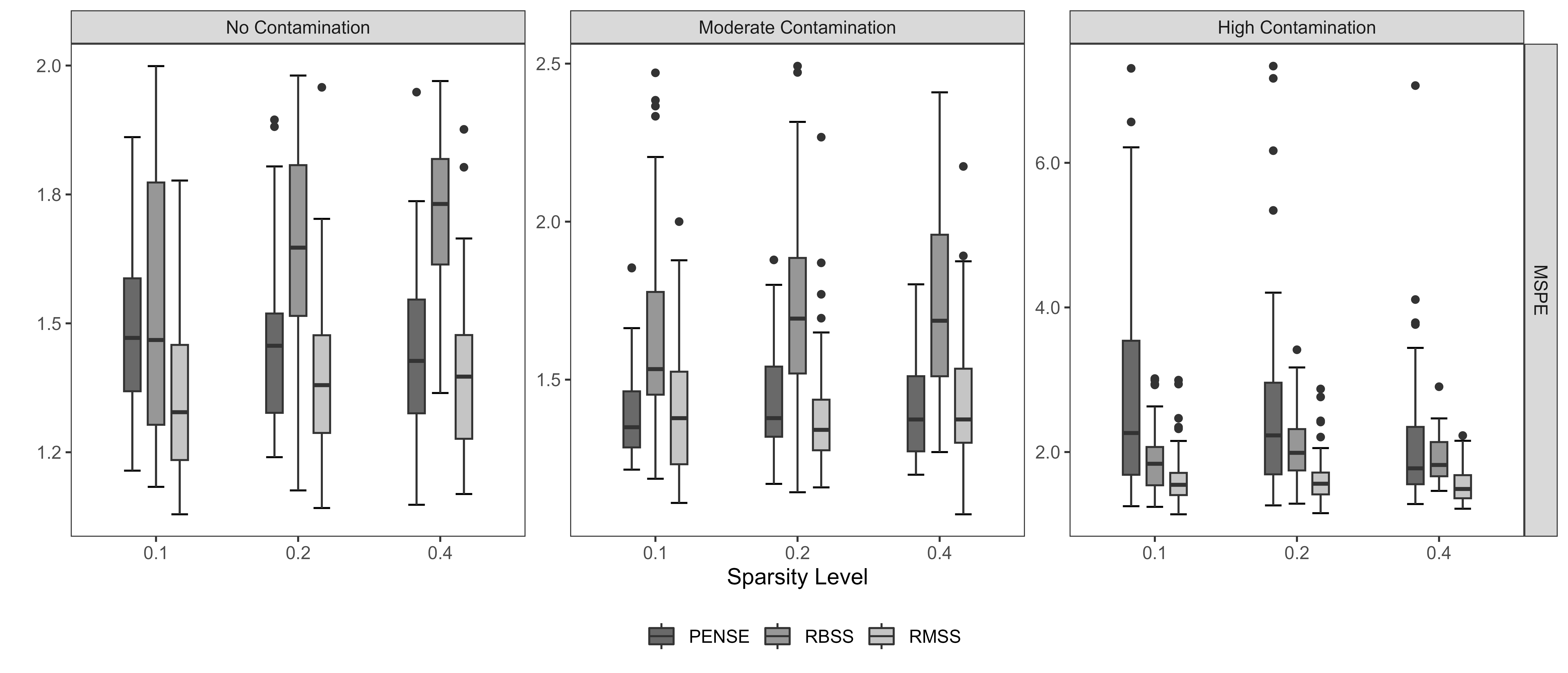
Figure 1: MSPE of PENSE, RBSS and RMSS over $N=50$ random training sets over different contamination and sparsity levels for $\text{SNR}=1$.

In Table 2 we report the average and lowest RC and PR rank of the six methods over the nine possible combinations of the SNR and sparsity level for each contamination proportion. RMSS achieved the best average RC rank over all contamination levels, while PENSE was the second best performing method over all contamination levels. In terms of PR, RBSS was the best performing method. In particular, when the data was contaminated as RBSS always had the best PR while RMSS always had the second best PR.

In Figure 2 we plot the RC and PR of PENSE, RBSS and RMSS over the $N=50$ random training sets over different contamination and sparsity levels for a moderate signal. RMSS with $G=10$ models outperformed PENSE and RBSS in terms of RC over all contamination levels when $\zeta=0.1$ and 0.2, and was competitive with PENSE when $\zeta=0.4$. In our numerical experiments, RMSS achieved even superior RC when we used more than $G=10$ models. RBSS generally had the best performance in terms of PR, however the RC of RBSS was subpar over any combination of sparsity, contamination and SNR level. RMSS combined a high RC with a high PR which remained stable across all configurations of our simulation study, an impressive feat in a simulation that combined a high-dimensional block correlation structure with regression outliers. The excellent performance of RMSS in terms of RC and PR was also observed in the low and high SNR scenarios.

Table 2: Average and lowest RC and PR rank of the six methods over the nine SNR and sparsity level combinations for each contamination proportion.

=2pt RC Rank PR Rank $\mathbf{\boldsymbol{\tau}=0}$ $\mathbf{\boldsymbol{\tau}=0.15}$ $\mathbf{\boldsymbol{\tau}=0.3}$ $\mathbf{\boldsymbol{\tau}=0}$ $\mathbf{\boldsymbol{\tau}=0.15}$ $\mathbf{\boldsymbol{\tau}=0.3}$ Method Avg Low Avg Low Avg Low Avg Low Avg Low Avg Low EN 5.4 6 5.7 6 5.3 6 2.1 4 5.7 6 5.3 6 PENSE 2.3 3 1.8 2 1.9 2 5.0 5 3.0 3 3.0 3 HuberEN 2.3 3 5.1 6 5.7 6 3.7 4 5.3 6 5.7 6 SparseLTS 5.4 6 4.1 5 4.0 4 6.0 6 4.0 4 4.0 4 RBSS 4.1 5 3.1 4 3.3 3 1.2 2 1.0 1 1.0 1 RMSS 1.7 3 1.2 2 1.1 2 3.0 4 2.0 2 2.0 2

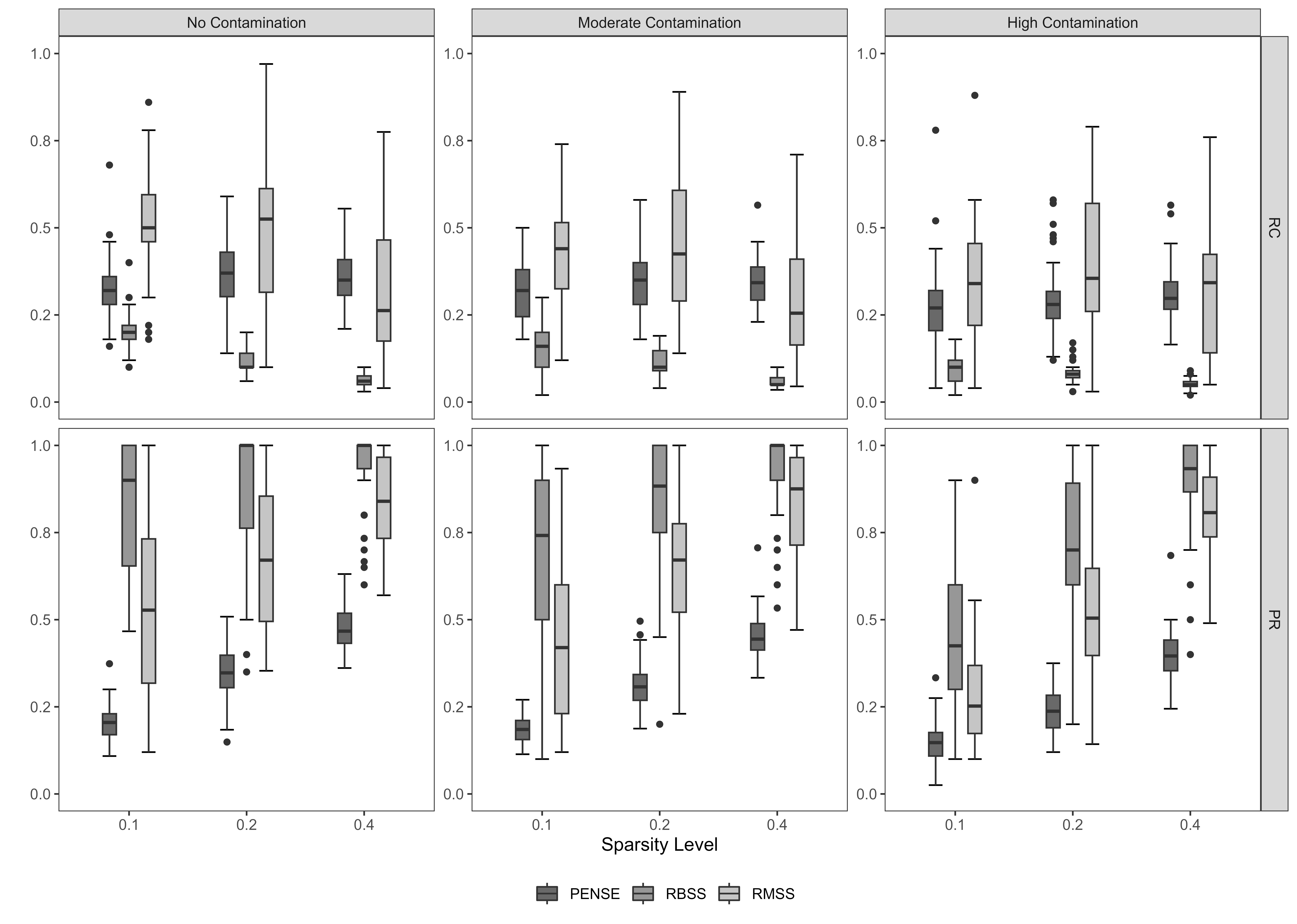
Figure 2: RC and PR of PENSE, RBSS and RMSS over $N=50$ random training sets over different contamination and sparsity levels for $\text{SNR}=1$.

6.6 Computing Times

The average computing times of the R function calls over all configurations of our simulation is given in Table 3. The R function call of RMSS given in Table 3 also includes the computation of RBSS since the latter is simultaneously computed by setting $u=G$ in (17). Our implementation of RMSS generates $G=10$ sparse and robust models simultaneously and still achieved a lower average computing time than PENSE, which generates a single sparse and robust model, with a smaller number of initial estimates than the default in its R implementation. Moreover RMSS must perform CV over three tuning parameters compared to only one for all the single-model sparse and robust methods.

The computing time of RMSS would increase significantly if it uses the neighborhood search strategy of Section 5.3. In general we find that the neighborhood search improves the solutions $\boldsymbol{\hat{\beta}}^{g}$ ($1\leq g\leq G$) in terms of variable selection and minimizing the objective function (17) but not in terms of out-of-sample prediction. We relay to the supplementary material our numerical experiment to compare the empirical performance and computational cost of RMSS with and without the neighborhood search.

Table 3: Computation time of R function calls for the methods in CPU seconds. CPU seconds are on a 2.7 GHz Intel Xeon processor in a machine running Linux 7.8 with 125 GB of RAM.

=2pt Method EN PENSE HuberEN SparseLTS RMSS Time 0.1 281.8 0.1 169.5 239.7

7 Contamination of Bioinformatics and Cheminformatics Data

In the omics sciences new deoxyribonucleic acid (DNA) microarray and ribonucleic acid (RNA) sequencing technologies allow for an increase in the type and volume of the omics data collected (see e.g. Gao et al., 2019; Syu et al., 2020; Hong et al., 2020; Wang et al., 2020; Okamura et al., 2023). The analysis of high-throughput omics data is a fundamental challenge in bioinformatics, and statistical methods are some of the primary tools used by scientists to tackle these challenges. In chemistry, innovative microscopic technologies allow for the collection of data on the composition of chemical compounds and molecules. The fields of statistics and machine learning have become indispensable for the analysis of complex chemical data, revolutionizing the field of cheminformatics (see e.g. Lo et al., 2018; von Lilienfeld and Burke, 2020; Kuntz and Wilson, 2022).

Many modern datasets with biological or chemical information are high-dimensional and display some form of data contamination. For example in bioinformatics many datasets collected through microarray technology are prone to cross-contamination resulting in samples with poor measurement quality (see e.g. Stkepniak et al., 2013). Next generation sequencing (NGS) technologies can efficiently generate high-dimensional genomic, proteomic, transcriptomic and epigenomic data, however such tools can sometimes produce a significant amount of incorrect reads (see e.g. Sangiovanni et al., 2019). Such dataset require statistical tools that can handle a large number of measurements and potentially contaminated samples. In cheminformatics the topic of high-dimensionality and robustness has gained a lot of attention in recent years due to the emerging fields of computer-aided drug design and computational toxicology among others (see e.g. Basak and Vracko, 2022).

In this section we artificially contaminate real bioinformatic and cheminformatic datasets to evaluate the performance of RMSS and state-of-the-art sparse and robust methods in situations that mimic real data applications. We also show that RMSS can potentially uncover some predictor variables that may be relevant to predict the outcome of interest but that may not be picked up by single-model sparse and robust methods.

7.1 Bioinformatics Data

In a study analyzing the genetic basis of Bardet-Biedl syndrome (BBS), Scheetz et al. (2006) performed mutation and functional studies and identified TRIM32 (tripartite motif-containing protein 32) as a gene whose expression highly correlates with the incidence of BBS. The R package abess (Zhu et al., 2022) contains a dataset with the expression of TRIM32 and $p=500$ genes for 120 mammalian-eye tissue samples, which is a subset of the original dataset analyzed by Scheetz et al. (2006). The $p=500$ genes were selected from the 18,976 available genes based on their marginal correlation with TRIM32 and are used to predict the expression of TRIM32.

The normalized gene expression levels in the uncontaminated dataset are all below 10 in magnitude. We randomly split the samples $N=50$ times in a training set of size $n=50$ and a test set of size $m=70$. We contaminate 25% of the samples of each training set by replacing the expression of TRIM32 and 100 randomly selected predictor genes with a normal random variable with mean 25 and standard deviation 1. We evaluate the MSPE of the same six methods used in Section 6 on the uncontaminated test set. For RMSS we fix $h=\lfloor 0.75n\rfloor=37$ but keep the grid $T=\{0.3n,0.4n,0.5n\}=\{15,20,25\}$ for the sparsity parameter. For the other methods we use the same configurations as in Section 6.

The MSPE and standard deviation (SD) of the MSPE reported in Table 5 are relative to the lowest value attained by the six methods, thus the best possible value is 1. The two best performances for each measure is marked in bold. RMSS achieved the best performance in terms of MSPE with the lowest MSPE variability. Sparse LTS was the closest competitor but its MSPE was still 7% higher than the MSPE of RMSS. The individual $G=10$ models of RMSS also achieved a high prediction accuracy with an average MSPE only 10% higher than the MSPE of RBSS. This observation indicates that each individual model correctly identified the outlying samples (see Corollary 2). Conversely the EN completely deteriorated with the addition of the outliers to the data.

Table 4: MSPE and SD of the six methods relative to the best performance for the artificially contaminated BBS bioinformatic dataset.

=2pt Method EN PENSE HuberEN SparseLTS RBSS RMSS MSPE $>25$ 1.11 1.26 1.07 1.77 1.00 SD $>100$ 1.40 1.64 1.26 4.11 1.00

Beyond the good predictive performance of RMSS, the ensembles can potentially uncover genes that are not identified by the other methods. In particular, in the presence of high-dimensional data there are multiple models comprised of different subsets of predictors that can each achieve a high prediction accuracy. This phenomenon is known as the ‘the multiplicity of good models” in the statistical literature (see relevant discussions in McCullagh and Nelder, 1989; Mountain and Hsiao, 1989). Thus single-model sparse and robust methods may potentially discard important genes from the decision-making process. On the BBS dataset, no gene was selected more than 50% of the time by PENSE or Sparse LTS over the $N=50$ random training sets, while 30 genes were selected more than 50% of the time by RMSS. Moreover the genes most often selected by PENSE and Sparse LTS were often selected by RMSS. For example PENSE selected gene at probe 13704291_at most often, and this gene was selected the same number of times by RMSS. Conversely, the genes most often selected by RMSS were seldom selected by PENSE or Sparse LTS. For example, the gene at probe 1374809_at was selected 72% of the time by RMSS and only 2% and 4% of the time by PENSE and Sparse LTS respectively.

7.2 Cheminformatics Data

We analyze the glass dataset from Lemberge et al. (2000) for which the goal is to predict the concentration of the chemical compound Na2O based on its frequency measurements obtained from an electron probe X-ray microanalysis (EPXMA). After removing variables with little variation, the dataset is comprised of $p=486$ frequency measurements for $n=180$ samples. We split the data into $N=50$ training sets of size $n=50$ and test sets of size $m=130$. We contaminate the training sets in the same way as we did for the BBS data, and compute the MSPE of the methods using the uncontaminated test sets. We use the same configuration of the methods as for the BBS dataset.

In Table 4 we report the MSPE and SD of the MSPE of the methods relative to the best performing method. RMSS again achieved the best MSPE by far as Sparse LTS coming was the second method with an MSPE 54% larger. RMSS was also the most stable method in terms of prediction accuracy. The $G=10$ individual models of RMSS achieved an MSPE similar to RBSS (only 3% larger). The good predictive performance of RMSS is not restricted to the chemical compound Na2O and may be observed in more compounds available in Lemberge et al. (2000).

Table 5: MSPE and SD of the six methods relative to the best performance for the artificially contaminated glass cheminformatic dataset.

=2pt Method EN PENSE HuberEN SparseLTS RBSS RMSS MSPE $>150$ 1.90 10.91 1.54 2.58 1.00 SD $>300$ 2.62 7.04 1.28 3.86 1.00

RMSS also uncovered frequency measurements that may be relevant to predict the concentration of Na2O that were missed by PENSE and Sparse LTS. The frequency measurement most often selected by RMSS (92% of the time over the $N=50$ random training sets) was only selected 2% of the time by both PENSE and Sparse LTS. On the other hand, the frequency measurements most often selected by PENSE and Sparse LTS were often selected by RMSS. In fact, the frequency measurement most often selected by PENSE was selected only 30% of the time, and this same frequency measurement was selected 90% of the time by RMSS.

8 Cardiac Allograft Vasculopathy Data Application

9 Summary and Future Works

In this article we introduced RMSS, a data-driven method to learn an ensemble of sparse and robust models directly from the data without any form of heuristics, the first of its kind in the literature. The degree to which the models are sparse, diverse and robust is driven directly by the data based on a CV criterion. We established the finite-sample breakdown point of the ensembles and the individual models within the ensembles. To bypass the NP-hard computational complexity of RMSS we developed a tailored computing algorithm with a local convergence property by leveraging recent developments in the $\ell_{0}$-optimization literature. Our extensive numerical experiments on synthetic and real data demonstrate the excellent performance of RMSS relative to state-of-the-art sparse and robust methods in high-dimensional prediction tasks when the data is also contaminated. We also showed how RMSS can potentially uncover important predictor variables that may be discarded by single-model sparse and robust methods.

Since RMSS can potentially uncover predictor variables that are not picked up by single-model methods, the addition of interaction terms may potentially further increase the competitive advantage of RMSS over single-model sparse and robust methods. Interaction terms are often statistically relevant e.g. in the omics sciences where interactions between genes or proteins may drive the outcome of interest. The empirical performance of RMSS could be improved further by considering alternative ways to combine the models in the ensembles other than the simple model average we used in this article.

With the growing emphasis on interpretable statistical and machine learning algorithms in the literature and in real data applications, our proposal will potentially pave the way for new exciting proposals in the area of data-driven robust ensemble modeling. A potential bottleneck in this area of research is the high computational cost of such methods, thus new optimization tools and methods will be needed to render such ensemble methods relevant in practice. Alternative robust loss functions may also be used more generally in the objective function.

Conflict of Interests

The authors declare no potential conflict of interests.

References

- Akaike (1974) Akaike, H. (1974). A new look at the statistical model identification. IEEE Transactions on Automatic Control 19(6), 716–723.
- Alfons (2021) Alfons, A. (2021). robustHD: An R package for robust regression with high-dimensional data. Journal of Open Source Software 6(67), 3786.
- Alfons et al. (2013) Alfons, A., C. Croux, and S. Gelper (2013). Sparse least trimmed squares regression for analyzing high-dimensional large data sets. The Annals of Applied Statistics, 226–248.
- Atkinson and Cheng (1999) Atkinson, A. C. and T.-C. Cheng (1999). Computing least trimmed squares regression with the forward search. Statistics and Computing 9(4), 251–263.
- Basak and Vracko (2022) Basak, S. C. and M. Vracko (2022). Big Data Analytics in Chemoinformatics and Bioinformatics: With Applications to Computer-Aided Drug Design, Cancer Biology, Emerging Pathogens and Computational Toxicology. Elsevier.
- Bertsimas et al. (2016) Bertsimas, D., A. King, and R. Mazumder (2016). Best subset selection via a modern optimization lens. The Annals of Statistics 44(2), 813–852.
- Bertsimas and Van Parys (2020) Bertsimas, D. and B. Van Parys (2020). Sparse high-dimensional regression: Exact scalable algorithms and phase transitions. The Annals of Statistics 48(1), 300–323.
- Biau et al. (2016) Biau, G., A. Fischer, B. Guedj, and J. D. Malley (2016). Cobra: A combined regression strategy. Journal of Multivariate Analysis 146, 18–28.
- Breiman (1996a) Breiman, L. (1996a). Bagging predictors. Machine Learning 24(2), 123–140.
- Breiman (1996b) Breiman, L. (1996b). Stacked regressions. Machine Learning 24(1), 49–64.
- Breiman (2001) Breiman, L. (2001, October). Random forests. Machine Learning 45(1), 5–32.
- Bühlmann and Van De Geer (2011) Bühlmann, P. and S. Van De Geer (2011). Statistics for high-dimensional data: methods, theory and applications. Springer Science & Business Media.
- Bühlmann and Yu (2003) Bühlmann, P. and B. Yu (2003). Boosting with the l 2 loss: regression and classification. Journal of the American Statistical Association 98(462), 324–339.
- Bunea et al. (2007) Bunea, F., A. B. Tsybakov, and M. H. Wegkamp (2007). Aggregation for gaussian regression. The Annals of Statistics 35(4), 1674–1697.
- Chandra et al. (2001) Chandra, R., L. Dagum, D. Kohr, R. Menon, D. Maydan, and J. McDonald (2001). Parallel programming in OpenMP. Morgan Kaufmann.
- Chen and Guestrin (2016) Chen, T. and C. Guestrin (2016). Xgboost: A scalable tree boosting system. In Proceedings of the 22nd acm sigkdd international conference on knowledge discovery and data mining, pp. 785–794.
- Christidis and Cohen-Freue (2023a) Christidis, A. and G. Cohen-Freue (2023a). RMSS: Robust Multi-Model Subset Selection. R package version 1.1.1.
- Christidis and Cohen-Freue (2023b) Christidis, A. and G. Cohen-Freue (2023b). robStepSplitReg: Robust Stepwise Split Regularized Regression. R package version 1.1.0.
- Christidis et al. (2023) Christidis, A.-A., S. V. Aelst, and R. Zamar (2023). Multi-model subset selection.
- Christidis et al. (2020) Christidis, A.-A., L. Lakshmanan, E. Smucler, and R. Zamar (2020). Split regularized regression. Technometrics 62(3), 330–338.
- Cohen Freue et al. (2019) Cohen Freue, G. V., D. Kepplinger, M. Salibián-Barrera, and E. Smucler (2019). Robust elastic net estimators for variable selection and identification of proteomic biomarkers.
- Ding and Xu (2014) Ding, H. and J. Xu (2014). Sub-linear time hybrid approximations for least trimmed squares estimator and related problems. In Proceedings of the thirtieth annual symposium on Computational geometry, pp. 110–119.
- Donoho and Huber (1983) Donoho, D. L. and P. J. Huber (1983). The notion of breakdown point. A festschrift for Erich L. Lehmann 157184.
- Efron et al. (2004) Efron, B., T. Hastie, I. Johnstone, and R. Tibshirani (2004). Least angle regression. The Annals of Statistics 32(2), 407–499.
- Fischer and Mougeot (2019) Fischer, A. and M. Mougeot (2019). Aggregation using input–output trade-off. Journal of Statistical Planning and Inference 200, 1–19.
- Friedman et al. (2007) Friedman, J., T. Hastie, H. Höfling, and R. Tibshirani (2007). Pathwise coordinate optimization. The Annals of Applied Statistics 1(2), 302–332.
- Friedman (2001) Friedman, J. H. (2001). Greedy function approximation: A gradient boosting machine. Ann. Statist. 29(5), 1189–1232.
- Friedman et al. (2010) Friedman, J. H., T. Hastie, and R. Tibshirani (2010). Regularization paths for generalized linear models via coordinate descent. Journal of Statistical Software 33(1), 1.
- Gao et al. (2019) Gao, C., M. Wei, T. R. McKitrick, A. M. McQuillan, J. Heimburg-Molinaro, and R. D. Cummings (2019). Glycan microarrays as chemical tools for identifying glycan recognition by immune proteins. Frontiers in chemistry 7, 833.
- Garside (1965) Garside, M. (1965). The best sub-set in multiple regression analysis. Journal of the Royal Statistical Society: Series C (Applied Statistics) 14(2-3), 196–200.
- Giloni and Padberg (2002) Giloni, A. and M. Padberg (2002). Least trimmed squares regression, least median squares regression, and mathematical programming. Mathematical and Computer Modelling 35(9-10), 1043–1060.
- Hastie et al. (2020) Hastie, T., R. Tibshirani, and R. Tibshirani (2020). Best subset, forward stepwise or lasso? analysis and recommendations based on extensive comparisons. Statistical Science 35(4), 579–592.
- Hastie et al. (2019) Hastie, T., R. Tibshirani, and M. Wainwright (2019). Statistical learning with sparsity: the lasso and generalizations. Chapman and Hall/CRC.
- Hawkins (1994) Hawkins, D. M. (1994). The feasible solution algorithm for least trimmed squares regression. Computational statistics & data analysis 17(2), 185–196.
- Hazimeh and Mazumder (2020) Hazimeh, H. and R. Mazumder (2020). Fast best subset selection: Coordinate descent and local combinatorial optimization algorithms. Operations Research 68(5), 1517–1537.
- Ho (1998) Ho, T. K. (1998). The random subspace method for constructing decision forests. IEEE Transactions on Pattern Analysis and Machine Intelligence 20(8), 832–844.
- Hong et al. (2020) Hong, M., S. Tao, L. Zhang, L.-T. Diao, X. Huang, S. Huang, S.-J. Xie, Z.-D. Xiao, and H. Zhang (2020). Rna sequencing: new technologies and applications in cancer research. Journal of hematology & oncology 13(1), 1–16.
- Huber (1964) Huber, P. J. (1964). Robust estimation of a location parameter. Annals of Mathematical Statistics 2, 73–101.
- Kenney et al. (2021) Kenney, A., F. Chiaromonte, and G. Felici (2021). Mip-boost: Efficient and effective l 0 feature selection for linear regression. Journal of Computational and Graphical Statistics 30(3), 566–577.
- Kepplinger (2023) Kepplinger, D. (2023). Robust variable selection and estimation via adaptive elastic net s-estimators for linear regression. Computational Statistics & Data Analysis 183, 107730.
- Kepplinger et al. (2023) Kepplinger, D., M. Salibián-Barrera, and G. Cohen Freue (2023). pense: Penalized Elastic Net S/MM-Estimator of Regression. R package version 2.2.0.
- Khan et al. (2007a) Khan, J. A., S. Van Aelst, and R. H. Zamar (2007a). Building a robust linear model with forward selection and stepwise procedures. Computational Statistics & Data Analysis 52(1), 239–248.
- Khan et al. (2007b) Khan, J. A., S. Van Aelst, and R. H. Zamar (2007b). Robust linear model selection based on least angle regression. Journal of the American Statistical Association 102(480), 1289–1299.
- Koller and Stahel (2017) Koller, M. and W. A. Stahel (2017). Nonsingular subsampling for regression s estimators with categorical predictors. Computational Statistics 32, 631–646.
- Kuntz and Wilson (2022) Kuntz, D. and A. K. Wilson (2022). Machine learning, artificial intelligence, and chemistry: How smart algorithms are reshaping simulation and the laboratory. Pure and Applied Chemistry 94(8), 1019–1054.
- Lemberge et al. (2000) Lemberge, P., I. De Raedt, K. H. Janssens, F. Wei, and P. J. Van Espen (2000). Quantitative analysis of 16–17th century archaeological glass vessels using pls regression of epxma and -xrf data. Journal of Chemometrics: A Journal of the Chemometrics Society 14(5-6), 751–763.
- Li (2005) Li, L. M. (2005). An algorithm for computing exact least-trimmed squares estimate of simple linear regression with constraints. Computational statistics & data analysis 48(4), 717–734.
- Lo et al. (2018) Lo, Y.-C., S. E. Rensi, W. Torng, and R. B. Altman (2018). Machine learning in chemoinformatics and drug discovery. Drug discovery today 23(8), 1538–1546.
- Mallows (1973) Mallows, C. L. (1973). Some comments on cp. Technometrics 15(4), 661–675.
- Maronna (2011) Maronna, R. A. (2011). Robust ridge regression for high-dimensional data. Technometrics 53(1), 44–53.
- Maronna et al. (2019) Maronna, R. A., R. D. Martin, V. J. Yohai, and M. Salibián-Barrera (2019). Robust statistics: theory and methods (with R). John Wiley & Sons.
- Maronna and Zamar (2002) Maronna, R. A. and R. H. Zamar (2002). Robust estimates of location and dispersion for high-dimensional datasets. Technometrics 44(4), 307–317.
- McCullagh and Nelder (1989) McCullagh, P. and J. A. Nelder (1989). Monographs on statistics and applied probability. Generalized Linear Models 37.
- Meinshausen (2007) Meinshausen, N. (2007). Relaxed lasso. Computational Statistics & Data Analysis 52(1), 374–393.
- Mountain and Hsiao (1989) Mountain, D. and C. Hsiao (1989). A combined structural and flexible functional approach for modeling energy substitution. Journal of the American Statistical Association 84(405), 76–87.
- Okamura et al. (2023) Okamura, H., H. Yamano, T. Tsuda, J. Morihiro, K. Hirayama, and H. Nagano (2023). Development of a clinical microarray system for genetic analysis screening. Practical Laboratory Medicine 33, e00306.
- Peña and Yohai (1999) Peña, D. and V. Yohai (1999). A fast procedure for outlier diagnostics in large regression problems. Journal of the American Statistical Association 94(446), 434–445.
- Pope and Webster (1972) Pope, P. and J. Webster (1972). The use of an f-statistic in stepwise regression procedures. Technometrics 14(2), 327–340.
- R Core Team (2022) R Core Team (2022). R: A Language and Environment for Statistical Computing. Vienna, Austria: R Foundation for Statistical Computing.
- Raymaekers and Rousseeuw (2021) Raymaekers, J. and P. J. Rousseeuw (2021). Fast robust correlation for high-dimensional data. Technometrics 63(2), 184–198.
- Rousseeuw and Yohai (1984) Rousseeuw, P. and V. Yohai (1984). Robust regression by means of s-estimators. In Robust and Nonlinear Time Series Analysis: Proceedings of a Workshop Organized by the Sonderforschungsbereich 123 “Stochastische Mathematische Modelle”, Heidelberg 1983, pp. 256–272. Springer.
- Rousseeuw (1984) Rousseeuw, P. J. (1984). Least median of squares regression. Journal of the American statistical association 79(388), 871–880.
- Rousseeuw and Bossche (2018) Rousseeuw, P. J. and W. V. D. Bossche (2018). Detecting deviating data cells. Technometrics 60(2), 135–145.
- Rousseeuw and Leroy (2005) Rousseeuw, P. J. and A. M. Leroy (2005). Robust regression and outlier detection. John wiley & sons.
- Rousseeuw and Van Driessen (2006) Rousseeuw, P. J. and K. Van Driessen (2006). Computing lts regression for large data sets. Data mining and knowledge discovery 12, 29–45.
- Salibian-Barrera and Yohai (2006) Salibian-Barrera, M. and V. J. Yohai (2006). A fast algorithm for s-regression estimates. Journal of computational and Graphical Statistics 15(2), 414–427.
- Sangiovanni et al. (2019) Sangiovanni, M., I. Granata, A. S. Thind, and M. R. Guarracino (2019). From trash to treasure: detecting unexpected contamination in unmapped ngs data. BMC bioinformatics 20(4), 1–12.
- Schapire and Freund (2012) Schapire, R. E. and Y. Freund (2012). Boosting: Foundations and Algorithms. The MIT Press.
- Scheetz et al. (2006) Scheetz, T. E., K.-Y. A. Kim, R. E. Swiderski, A. R. Philp, T. A. Braun, K. L. Knudtson, A. M. Dorrance, G. F. DiBona, J. Huang, T. L. Casavant, et al. (2006). Regulation of gene expression in the mammalian eye and its relevance to eye disease. Proceedings of the National Academy of Sciences 103(39), 14429–14434.
- Shen et al. (2013) Shen, X., W. Pan, Y. Zhu, and H. Zhou (2013). On constrained and regularized high-dimensional regression. Annals of the Institute of Statistical Mathematics 65(5), 807–832.
- Smucler and Yohai (2017) Smucler, E. and V. J. Yohai (2017). Robust and sparse estimators for linear regression models. Computational Statistics & Data Analysis 111, 116–130.
- Song et al. (2013) Song, L., P. Langfelder, and S. Horvath (2013). Random generalized linear model: a highly accurate and interpretable ensemble predictor. BMC Bioinformatics 14(1), 5.
- Stkepniak et al. (2013) Stkepniak, P., M. Maycock, K. Wojdan, M. Markowska, S. Perun, A. Srivastava, L. S. Wyrwicz, and K. Swirski (2013). Microarray inspector: tissue cross contamination detection tool for microarray data. Acta Biochimica Polonica 60(4).
- Syu et al. (2020) Syu, G.-D., J. Dunn, and H. Zhu (2020). Developments and applications of functional protein microarrays. Molecular & Cellular Proteomics 19(6), 916–927.
- Takano and Miyashiro (2020) Takano, Y. and R. Miyashiro (2020). Best subset selection via cross-validation criterion. Top 28(2), 475–488.
- Thompson (2022) Thompson, R. (2022). Robust subset selection. Computational Statistics & Data Analysis, 107415.
- Tibshirani (1996) Tibshirani, R. (1996). Regression shrinkage and selection via the lasso. Journal of the Royal Statistical Society: Series B (Statistical Methodological) 58(1), 267–288.
- Ueda and Nakano (1996) Ueda, N. and R. Nakano (1996). Generalization error of ensemble estimators. In Proceedings of International Conference on Neural Networks (ICNN’96), Volume 1, pp. 90–95. IEEE.
- Van De Geer and Bühlmann (2009) Van De Geer, S. A. and P. Bühlmann (2009). On the conditions used to prove oracle results for the lasso. Electronic Journal of Statistics 3, 1360–1392.
- Van der Laan et al. (2007) Van der Laan, M. J., E. C. Polley, and A. E. Hubbard (2007). Super learner. Statistical applications in genetics and molecular biology 6(1).
- von Lilienfeld and Burke (2020) von Lilienfeld, O. A. and K. Burke (2020). Retrospective on a decade of machine learning for chemical discovery. Nature communications 11(1), 4895.
- Wang et al. (2020) Wang, Y., M. Mashock, Z. Tong, X. Mu, H. Chen, X. Zhou, H. Zhang, G. Zhao, B. Liu, and X. Li (2020). Changing technologies of rna sequencing and their applications in clinical oncology. Frontiers in oncology 10, 447.
- Welch (1982) Welch, W. J. (1982). Algorithmic complexity: three np-hard problems in computational statistics. Journal of Statistical Computation and Simulation 15(1), 17–25.
- Yi (2017) Yi, C. (2017). hqreg: Regularization Paths for Lasso or Elastic-Net Penalized Huber Loss Regression and Quantile Regression. R package version 1.4.
- Yi and Huang (2017) Yi, C. and J. Huang (2017). Semismooth newton coordinate descent algorithm for elastic-net penalized huber loss regression and quantile regression. Journal of Computational and Graphical Statistics 26(3), 547–557.
- Yohai (1987) Yohai, V. J. (1987). High breakdown-point and high efficiency robust estimates for regression. The Annals of statistics, 642–656.
- Zhang and Coombes (2012) Zhang, J. and K. R. Coombes (2012). Sources of variation in false discovery rate estimation include sample size, correlation, and inherent differences between groups. BMC Bioinformatics 13(S13), S1.
- Zhu et al. (2022) Zhu, J., X. Wang, L. Hu, J. Huang, K. Jiang, Y. Zhang, S. Lin, and J. Zhu (2022). abess: a fast best-subset selection library in python and r. The Journal of Machine Learning Research 23(1), 9206–9212.
- Zhu et al. (2020) Zhu, J., C. Wen, J. Zhu, H. Zhang, and X. Wang (2020). A polynomial algorithm for best-subset selection problem. Proceedings of the National Academy of Sciences 117(52), 33117–33123.
- Zou (2006) Zou, H. (2006). The adaptive lasso and its oracle properties. Journal of the American Statistical Association 101(476), 1418–1429.
- Zou and Hastie (2005) Zou, H. and T. Hastie (2005). Regularization and variable selection via the elastic net. Journal of the Royal Statistical Society: Series B (Statistical Methodological) 67(2), 301–320.