Large Language Model-Enhanced Algorithm Selection:
Towards Comprehensive Algorithm Representation

Abstract

Algorithm selection, a critical process of automated machine learning, aims to identify the most suitable algorithm for solving a specific problem prior to execution. Mainstream algorithm selection techniques heavily rely on problem features, while the role of algorithm features remains largely unexplored. Due to the intrinsic complexity of algorithms, effective methods for universally extracting algorithm information are lacking. This paper takes a significant step towards bridging this gap by introducing Large Language Models (LLMs) into algorithm selection for the first time. By comprehending the code text, LLM not only captures the structural and semantic aspects of the algorithm, but also demonstrates contextual awareness and library function understanding. The high-dimensional algorithm representation extracted by LLM, after undergoing a feature selection module, is combined with the problem representation and passed to the similarity calculation module. The selected algorithm is determined by the matching degree between a given problem and different algorithms. Extensive experiments validate the efficacy of the proposed model and especially illustrate its generalization capability over algorithms. Furthermore, we provide theoretical upper bounds for the generalization error over both problems and algorithms, highlighting a significant superiority conferred by the algorithm representation.

1 Introduction

Performance complementarity, a phenomenon where no single algorithm consistently outperforms all others across diverse problem instances, is a well-established reality in the realm of optimization and learning problems Kerschke et al. (2019). Over the past few years, the growing interest in automated algorithm selection techniques has become evident. These techniques aim to tackle the challenge of selecting the most appropriate algorithm from a predefined set for a given problem instance automatically Ruhkopf et al. (2022); Heins et al. (2023). Most existing techniques rely on two sources of information: (1) the features of each problem instance and (2) the historical performance of various algorithms across problem instances Pio et al. (2023). Then, regression Xu et al. (2008) or ranking Abdulrahman et al. (2018) based machine learning models are used to establish a mapping from problem features to algorithm performance or the best-performing algorithm. Additionally, there are also methods based on collaborative filtering Mısır and Sebag (2017) or instance similarity Amadini et al. (2014).

Many contemporary algorithm selection methodologies predominantly treat algorithms as black boxes, concentrating primarily on the features of given problems. Nonetheless, it is essential to acknowledge that, for the majority of scenarios, algorithm feature constitutes a vital source of information, and overlooking it may lead to performance degradation Tornede et al. (2020). Relying exclusively on problem features limits the model to learning a unidirectional mapping from the problem to the algorithm, which does not align with the potentially bidirectional nature of the problem-algorithm relationships. An ideal algorithm selection model should not only identify the suitable algorithm for a given problem but also understand the types of problems for which an algorithm is well-suited, i.e., the interactive synthesis of problem representation and algorithm representation.

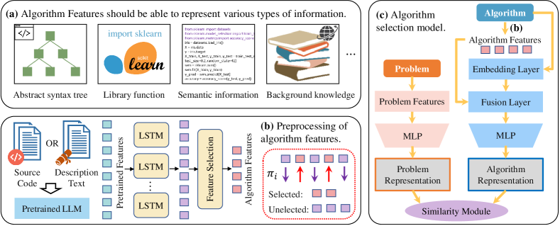
Figure 1: The framework of AS-LLM: (a) illustrates the various types of information that influence algorithm representation. (b) shows the algorithm features extracted by LLM and their preprocessing using feature selection. (c) outlines the proposed algorithm selection framework.

The limited consideration given to algorithm features is primarily attributed to the following practical challenges. Firstly, the inherent complexity and diversity of algorithms make it difficult to develop a universally applicable method for algorithm representation. For instance, among the limited studies related to algorithm features, the majority of them manually design features pertaining to specific scenarios or algorithm types, such as features based on hyperparameters Hough and Williams (2006); Tornede et al. (2020), execution process Nobel et al. (2021), model structures, or loss functions Hilario et al. (2009). These features often have different meanings and scales even within the same category of algorithms, rendering them impractical for universal adaptation across diverse algorithm types. On the other hand, quantifying and elucidating algorithm features indeed presents a formidable challenge. The intricate logic and rich contextual information make it difficult to devise a feature extraction method that captures key algorithmic information. One notable endeavor involves using macro statistical features (e.g., lines of code) and abstract syntax tree (AST) features (e.g., node/edge count) of code to represent algorithms Pulatov et al. (2022). While these features can characterize the structural aspects of algorithms, they fall short of directly encapsulating semantic relationships and contextual information within the code. Additionally, certain core algorithms often depend on library functions, which exist at a higher level of abstraction and cannot be directly manifested in the AST. This discrepancy results in the masking of critical information.

With the advent of the pretrained Large Language Models (LLMs) era Ouyang et al. (2022), the extraction of algorithm features from code-related text has become significantly more attainable. LLMs exhibit three notable advantages in algorithm representation: (1) Rich and robust information content: LLMs not only encapsulate the syntax structure of code represented by AST but also capture nuanced semantic information and exhibit contextual awareness Guo et al. (2020), as shown in Figure 1(a), which allows algorithm features to maintain robustness across diverse programming languages. (2) Vast knowledge repository: LLMs leverage extensive knowledge from large-scale code repositories, enabling them to represent common patterns, library function usage, and module relationships Chen et al. (2021). This imparts superior domain adaptation capabilities to LLMs in the algorithm selection tasks. (3) Automation and universality: LLMs obviate the need for manual feature design as existing methods, but automatically extract features from code text, demonstrating universal applicability across various scenarios and algorithms. Even in scenarios where code is unavailable, LLMs can extract pertinent information from algorithm description text (e.g., pseudo-code).

Leveraging the powerful representation capability of LLMs, we introduce the proposed Algorithm Selection model based on LLM (AS-LLM). With the support of pretrained LLMs for code or text (e.g., Chen et al. (2021)), we efficiently represent the algorithm with minimal training overhead. Simultaneously, it is worth noting that LLM-based representations possess high dimensions Chen et al. (2021), and not all features are directly relevant to algorithm selection tasks. To further enhance the model, we integrate a feature selection module depicted in Figure 1(b), which carefully scrutinizes the pretrained features and extracts a subset of algorithm features that are most significant by deriving importance weights for them. Moreover, AS-LLM does not directly concatenate algorithm and problem features for performance regression. Instead, it adopts distinct treatment methodologies for these two feature types, as shown in Figure 1(c). Independent feature processing networks are employed to obtain problem and algorithm representations of equal length separately, which could mitigate premature interference between the two feature types. These representations are then intricately fused through similarity calculation modules, ultimately guiding the selection decision based on the matching degree between a given problem and different algorithms. The key contributions of this study are summarized as follows:

• To the best of our knowledge, this study represents a pioneering application of LLM in algorithm selection tasks, leveraging the powerful representation capability of LLM to extract discriminative algorithm features. We also introduce an algorithm feature selection module to identify critical features for algorithm selection.

• The comprehensive algorithm representation bestows AS-LLM with at least three advantages: (i) A more nuanced modeling of the bidirectional nature of algorithm selection tasks; (ii) The generalization capability to novel algorithms not encountered during training; (iii) Robust performance superiority in different scenarios.

• We not only highlight the potential of algorithm features to enhance the generalization across algorithms, but also provide a rigorous theoretical upper bound for generalization error when distribution shift occurs in both problems and algorithms within the test set.

2 Related Work

Algorithm selection aims to choose the appropriate algorithm for each problem instance from a set of algorithms Rice (1976). Traditionally, the problem of per-instance algorithm selection can be defined as follows: Given a problem set $P$, an algorithm set $A$ for solving problem instances in $P$, and a performance metric $\mathcal{M}$: $P\times A\rightarrow\mathbb{R}$ which quantifies the performance of any algorithm $a\in A$ on each instance $p\in P$, per-instance algorithm selection should construct a selector $\mathcal{S}:P\rightarrow A$ that assigns any problem instance $p\in P$ to an algorithm $a\in A$, optimizing the overall performance expectation $\mathbb{E}[\mathcal{M}(p,\mathcal{S}(p))]$ on $P$ according to the metric $\mathcal{M}$ Kerschke et al. (2019). In the following, we first review the classical types of algorithm selection techniques, followed by a focus on the study of algorithm features in existing works.

Regression-based techniques Xu et al. (2008) aim to predict the performance of different algorithms based on a set of features. Similarly, ranking-based approaches Cunha et al. (2018); Abdulrahman et al. (2018) assign a rank or score to each algorithm, indicating its relative suitability for a given problem. The ranking can be determined using various methods, such as pairwise comparisons or learning-to-rank algorithms. Some studies formalize algorithm selection as a collaborative filtering problem Mısır and Sebag (2017); Fusi et al. (2018) and utilize a sparse matrix with performance data of only a few algorithms on each problem instance. Similarity-based approaches Amadini et al. (2014); Kadioglu et al. (2010) select algorithms based on the similarity between the current problem instance and previously encountered instances. Moreover, hybrid methods Hanselle (2020); Fehring et al. (2022) combine multiple techniques above and leverage their strengths to improve the accuracy and robustness of algorithm selection. For more detailed information, please refer to Kerschke et al. (2019).

Currently, most research focuses on using problem features to achieve algorithm selection. Although there is relatively little literature on using algorithm features, there have been some attempts made in the following works. Hough and Williams are among the early researchers to consider the measurement of algorithm features. They extract hyperparameters of optimization algorithms and additionally construct five features to describe how algorithms handle optimization problems Hough and Williams (2006). Similarly, Tornede et al. [2020] discuss the feature representation of machine learning algorithms. They also employ the values of hyperparameters as algorithm features and then concatenate algorithm features and problem features to build a regression or ranking model. These features, along with problem features, are inputted into the decision tree and SVM models to identify the optimal algorithm for a problem instance. Hilario et al. suggest using information related to the structure, parameters, and cost function of a model as algorithm features without empirical study on this yet Hilario et al. (2009). Until recently, Pulatov et al. [2022] utilize macro-level features of code (e.g., lines of code and cyclomatic complexity), as well as abstract syntax tree features (e.g., the number of nodes and edges), to describe algorithm characteristics. This allows for the development of a unified model that can regress the performance of all algorithms, instead of building a separate regression model for each algorithm, as in their previous work. Moreover, Nobel et al. [2021] design a method for extracting time series features specifically for algorithm representation of Covariance Matrix Adaptation Evolution Strategy and its variants Hansen and Ostermeier (2001).

As analyzed in Section 1, these manually designed features either lack generality and only serve specific algorithm selection scenarios, or fail to fully capture the entire information of algorithms. This paper will introduce a novel algorithm representation technique based on the LLM and design a new framework for algorithm selection. Please refer to Tornede et al. (2023) for the application of LLM in other subareas of automated machine learning.

3 Algorithm Selection based on LLMs

This section introduces the main details of AS-LLM. As illustrated in Figure 1, AS-LLM primarily consists of three modules: the problem representation module, algorithm representation module, and similarity calculation module. Among them, the extraction and utilization of algorithm features are key aspects of this study. For each candidate algorithm, its corresponding code snippet is an easily accessible resource. Even in the absence of open-source code, the algorithm’s descriptive text (such as pseudo-code, papers, or manuals) is available and can serve as a viable alternative. Leveraging the code representation capability of pretrained LLMs, we aim to comprehensively extract and characterize the essence of each algorithm from their code-related texts. In this endeavor, the employed LLM can take on multiple forms, as long as its pretraining data contains code text. Hence, it can either be a general-purpose model pretrained on a vast corpus of text data (e.g., GPT-3 Floridi and Chiriatti (2020)) or a specialized model tailored for code comprehension and generation (e.g., CodeBERT Feng et al. (2020)). The model’s ability to comprehend code syntax, structure, and semantics allows it to identify critical algorithmic patterns and techniques. This entails recognizing loops, conditionals, data structures, and their interplay within the code.

Specifically, for $\forall a\in A$, algorithm indices are mapped to corresponding continuous vectors, obtained from a pretrained LLM:

$$\mathbf{E}_{a}=\text{LLM-Embedding}(a)\in\mathbb{R}^{e}$$ (1)

where $e$ is determined by the output scale of the chosen LLM. These embeddings can be frozen during training to preserve the knowledge encoded within them. When there is enough training data available, parameters in the LLM can be fine-turned together with the other parts of the model, and the embedding layer is updated according to the output of LLM. Given the sequential nature of algorithm features from LLM, we utilize an LSTM to handle these algorithm features:

$$\mathbf{H}_{a}=\text{LSTM}(\mathbf{E}_{a})$$ (2)

$$\mathbf{F}_{a}=\text{Linear}(\text{Concatenate}(\mathbf{h}_{-1},\mathbf{h}_{0}))$$

where $\mathbf{h}_{-1},\mathbf{h}_{0}\in\mathbf{H}_{a}$ are the LSTM encoder’s final hidden state and the initial hidden state. Herein, we chose to use LSTM instead of other advanced models such as Transformer primarily due to the limitations posed by the training data scale in the algorithm selection. While Transformer exhibits strong modeling capabilities for sequential data, it typically requires a larger amount of data for training. Given the finite number of candidate algorithms and the relatively small scale of the problems in algorithm selection tasks, the performance of the Transformer model could be constrained. In contrast, LSTM performs better when handling a small number of training samples.

As mentioned earlier, the representation of algorithm-related text by LLM is typically high-dimensional, which can range in the hundreds or thousands, there exists a disparity in dimensionality between algorithm features and problem features. Among these features, not all of them are relevant to the algorithm selection task. Therefore, it is necessary to add a feature selection module in front of the model’s main body to select the predictive features based on the task information. Herein, we first arrange a parameter $\pi_{i}$ to the $i$-th features in $\mathbf{F}_{a}$, which are the same in number as the features and indicate whether a feature should be selected. Then, we use Gumbel distributions to generate samples from classification distributions and make the feature selection operation differentiable. Specifically, for each parameter $\pi_{i}\in[0,1]$, we sample a random variable $\sigma^{+}_{i},\sigma^{-}_{i}\sim\text{Gumbel}(0,1)$ from the standard Gumbel distribution to obtain noise term. Then, according to its property,

$$\mathbb{P}(\log\pi_{i}+\sigma^{+}_{i}>\log(1-\pi_{i})+\sigma^{-}_{i})=\pi_{i}.$$ (3)

Using the softmax function as a continuous and differentiable approximation Jang et al. (2016), the $i$-th weighted feature ${\mathbf{F}^{\prime}_{a}}_{i}$ is:

$${\mathbf{F}^{\prime}_{a}}_{i}=\frac{\exp\left(\frac{\log\pi_{i}+\sigma^{+}_{i}}{\tau}\right)}{\exp\left(\frac{\log\pi_{i}+\sigma^{+}_{i}}{\tau}\right)+\exp\left(\frac{\log(1-\pi_{i})+\sigma^{-}_{i}}{\tau}\right)}{\mathbf{F}_{a}}_{i}.$$ (4)

where the weight indicates the probability of the $i$-th features being selected, and the parameter $\tau$ is the temperature parameter. When $\tau$ is greater than 0, it ensures the smoothness of the distribution and facilitates better gradients. As $\tau$ approaches 0, the values of $\mathbb{P}(i)$ converge towards $\pi_{i}$. Conversely, as $\tau$ approaches infinity, the probability tends toward a uniform distribution. For better practical usage, the feature selection module is trained together with other parts of the model. Based on the obtained values of the parameters $\pi_{i}$, the module selects the top-$k$ most important features. These selected features are then retained, and the feature selection module is removed. The other parts of the model are subsequently retrained without the feature selection module.

In addition to the pretrained features extracted by LLM, AS-LLM also utilizes an embedding layer to adaptively capture the algorithm representation:

$$\mathbf{E}^{\prime}_{a}=\text{Embedding}(a)\in\mathbb{R}^{k}$$ (5)

where $k$ indicates the same dimension with $\mathbf{F}^{\prime}_{a}$. This layer is directly learned from the matching relationship between the algorithm and the problem. Therefore, the embedding layer is only applicable when the candidate algorithm remains unchanged and can accurately represent the algorithms that have appeared in the training data. When the candidate algorithm remains unchanged, the adaptive features will bring performance gains in prediction. The adaptive features and pretrained features are fused in the fusion layer by weighted addition with a parameter $\alpha\in[0,1]$, resulting in an algorithm feature set $\mathbf{V}_{a}$. The problem features $\mathbf{F}_{p}$ and the algorithm features will each go through their respective multilayer perceptron (MLP) modules and then undergo a calculation of the cosine distance $d$:

$$\mathbf{V}_{p}=\text{MLP}_{P}(\mathbf{F}_{p})\in\mathbb{R}^{m}$$ (6)

$$\mathbf{V}_{a}=\text{MLP}_{A}\left[\alpha\mathbf{F}^{\prime}_{a}+(1-\alpha)\mathbf{E}^{\prime}_{a}\right]\in\mathbb{R}^{m}$$

$$d=\frac{\mathbf{V}_{a}\cdot\mathbf{V}_{p}}{\|\mathbf{V}_{a}\|\cdot\|\mathbf{V}_{p}\|}$$

Cosine similarity measures the cosine of the angle between these vectors and provides a score indicating their similarity. A higher $d$ suggests a better match between the problem and the algorithm. Finally, the cosine similarity is concatenated with problem features and algorithm features, and jointly influences the model’s final output through an MLP layer:

$$\text{Similarity}(a,p)=\text{MLP}_{S}\left[\text{Concatenate}(\mathbf{V}_{a},\mathbf{V}_{p},d)\right].$$ (7)

The model’s output $\text{Similarity}(a,p)$ is used to predict whether the input problem and algorithm are mutually compatible.

4 Upper Bound of Generalization Error

One of the key benefits of considering algorithm features is the potential for the model to exhibit generalization over candidate algorithms, enabling it to achieve considerable performance on previously unseen algorithms during the training process. While this advantage has been mentioned in prior research involving algorithm features Tornede et al. (2020), a theoretical upper bound on the generalization error has yet to be established. In this section, we bridge this gap based on the proposed AS-LLM model. It is important to note that, to enable generalization over new algorithms, both the embedding layer and the cosine distance calculation should be excluded from AS-LLM, denoted as AS-LLM_g. The rationale for removing the embedding layer has been previously discussed after Eq. (5). The elimination of the cosine distance calculation $d$, on the other hand, is primarily intended to establish a theoretical upper bound on the generalization error, which will be elucidated during the derivation process of Theorem 1 in this section.

Denote the space of AS-LLM_g as $\mathcal{F}$, $\mathbf{f}(x_{i})\in\mathcal{F}$ is a real-valued network mapping the instance $x_{i}$ to $\mathbb{R}$. For analytical convenience, we consider AS-LLM_g as a unified MLP, including all sub-MLPs either for problem representation, algorithm representation, or similarity calculation. This transformation is mathematically equivalent, as all parameters and activation functions in this unified MLP can be derived from the original model without extra computation. For instance, the parameters $W^{(1)}$ of the MLP’s first layer can be obtained by combining the parameters $W^{(1)}_{p}$ and $W^{(1)}_{a}$ from the $\text{MLP}_{P}$ and $\text{MLP}_{A}$ in Eq. (6), respectively, i.e., $W^{(1)}=\begin{pmatrix}W^{(1)}_{a}&O\\ O&W^{(1)}_{p}\\ \end{pmatrix}$. Similarly, each activation function also corresponds to its counterpart in the original model. Under this simplification, AS-LLM_g is treated as an MLP structure, facilitating the derivation of concise forms for the upper bounds of generalization error.

To investigate the generalization capability, we introduce the concept of inductive Rademacher Complexity Koltchinskii (2001) as a measure of the model’s complexity, which is calculated as:

$$\hat{\mathfrak{R}}_{|\mathcal{S}|}\left(\mathcal{F}\right)=\frac{1}{|\mathcal{S}|}\mathbf{E}_{\bm{\sigma}}\left[\sup_{\mathbf{f}\in\mathcal{F}}\sum_{x_{i}\in\mathcal{S}}\sigma_{i}\mathbf{f}\left(x_{i}\right)\right]$$ (8)

where $|\mathcal{S}|$ is the scale of training data $\mathcal{S}$, and $\bm{\sigma}=\{\sigma_{i}\}_{i=1}^{n}$ is an independent uniform $\{\pm 1\}$-valued random variables, $\sigma_{i}=1$ with probability $\frac{1}{2}$ and $\sigma_{i}=-1$ with the same probability. Inductive Rademacher Complexity is a concept used to quantify the model complexity. By examining it, we can gain an understanding of the model’s generalization ability and estimate the upper bound of its generalization error at a theoretical level. In the following, we first present an upper bound on the model complexity of AS-LLM_g in Theorem 1.

Theorem 1.

Let $|\mathcal{S}_{\mathcal{P}}|$ and $|\mathcal{S}_{\mathcal{A}}|$ denote the number of problems and algorithms in training samples, $W^{(i)}$ denote the parameter in the $i$-th layer with the upper bound of $F$-norm $R_{i}$, i.e., $\|W^{(i)}\|_{F}\leq R_{i}$, and $l$ denote the number of layers. Then, for the model $\mathbf{f}\left(x_{i}\right)$ with $1$-Lipschitz, positive-homogeneous activation functions, the inductive Rademacher complexity of AS-LLM_g is bounded by:

$$\hat{\mathfrak{R}}_{|\mathcal{S}|}\left(\mathcal{F}\right)\leq\frac{\sqrt{2l\log 2\Gamma_{\mathbf{f}}\Gamma_{\mathcal{S}}+2|\mathcal{S}_{\mathcal{P}}|^{\frac{1}{2}}|\mathcal{S}_{\mathcal{A}}|^{\frac{1}{2}}\Gamma^{2}_{\mathbf{f}}\Gamma_{\mathcal{S}}^{\frac{3}{2}}}}{\sqrt{|\mathcal{S}_{\mathcal{P}}|\cdot|\mathcal{S}_{\mathcal{A}}|}}$$ (9)

where $\Gamma_{\mathbf{f}}$ and $\Gamma_{\mathcal{S}}$ are model-related and data-related variables, denoted as:

$$\Gamma_{\mathbf{f}}=\prod_{i=1}^{l}R_{i},\ \ \Gamma_{\mathcal{S}}=\max_{x_{j}\in\mathcal{S}}\|x_{j}\|^{2}.$$ (10)

Proof.

Please refer to the Appendix A. ∎

The upper bound of $\hat{\mathfrak{R}}_{|\mathcal{S}|}\left(\mathcal{F}\right)$ can further lead to the bound of generalization error. In the following, we discuss the generalization performance of model AS-LLM_g in Theorem 2.

Theorem 2.

Follow the same definition in Theorem 1. Let $Error_{\mathcal{T}}(\mathbf{f})$ and $Error_{\mathcal{S}}(\mathbf{f})$ denote the test error and empirical error of the AS-LLM_g $\mathbf{f}\left(x_{i}\right)$. $\chi^{2}(P_{\mathcal{T}}\|P_{\mathcal{S}})=\int\frac{P^{2}_{\mathcal{T}}(x_{j})}{P_{\mathcal{S}}(x_{j})}-1$ denotes the chi-square divergence between distributions of training and test sets. If $\Gamma_{\mathbf{f}}>1$ and $\sqrt{|\mathcal{S}_{\mathcal{P}}|\cdot|\mathcal{S}_{\mathcal{A}}|}\gg(\log 2)l$, then with probability at least $1-\delta$ over the sample, for all margins $\gamma>0$ and all $\forall\mathbf{f}\in\mathcal{F}$ with $1$-Lipschitz, positive-homogeneous activation functions, we have,

$$Error_{\mathcal{T}}(\mathbf{f})\leq Error_{\mathcal{S}}(\mathbf{f})+\mathcal{O}\left(\frac{[\chi^{2}(P_{\mathcal{T}}\|P_{\mathcal{S}})+1]^{\frac{3}{4}}\Gamma_{\mathbf{f}}\Gamma_{\mathcal{S}}^{\frac{3}{4}}}{|\mathcal{S}_{\mathcal{P}}|^{\frac{1}{4}}|\mathcal{S}_{\mathcal{A}}|^{\frac{1}{4}}\gamma}\right).$$ (11)

Proof.

Please refer to the Appendix B. ∎

Theorem 2 provides a theoretical guarantee for the generalization capacity of AS-LLM over both algorithms and problems, since the distribution shift on both problems and algorithms is considered by the chi-square divergence between distributions of training and test sets. Furthermore, the two weak assumptions in Theorem 2, i.e., $\Gamma_{\mathbf{f}}>1$ and $\sqrt{|\mathcal{S}|}\gg(\log 2)l$, could be satisfied in the majority of scenarios. They do not impose limitations on the scope of the theorem but serves primarily to ensure theoretical correctness.

According to Theorem 2, we can observe that the inductive generalization error is related to four factors: the training scale $|\mathcal{S}_{\mathcal{P}}|\cdot|\mathcal{S}_{\mathcal{A}}|$, the model parameter-related factor $\Gamma_{\mathbf{f}}$ and $\gamma$, training data-related factor $\Gamma_{\mathcal{S}}$, and the distribution difference between training and test set $\chi^{2}(P_{\mathcal{T}}\|P_{\mathcal{S}})$. It can offer practical assistance in at least two aspects: (1) Chi-square divergence: The generalization error gradually increases at a rate of $\mathcal{O}\left([\chi^{2}(P_{\mathcal{T}}\|P_{\mathcal{S}})+1]^{\frac{3}{4}}\right)$. By calculating this divergence, we can estimate the performance of AS-LLM_g before execution, especially in the case where new candidate algorithms are considered. The chi-square divergence can also be leveraged to select suitable LLM for algorithm feature extraction, by minimizing the disparities between the training and test sets. (2) Training set size: We observe that both the problem and algorithm sizes in the training set contribute to improved generalization performance, at a rate of $\mathcal{O}\left(|\mathcal{S}_{\mathcal{P}}|^{-\frac{1}{4}}|\mathcal{S}_{\mathcal{A}}|^{-\frac{1}{4}}\right)$. The generalization capacity can be estimated based on the number of candidate algorithms and problem instances in the training set. In practical applications, Theorem 2 can be employed to estimate the scale of training data needed.

5 Experiments

We first introduce the experimental setup, followed by presenting the results of the comparison and ablation study. The validation of LLM-extracted features and generalization capacity are provided in Appendix C and Appendix D.

Table 1: The statistical property of experimental benchmarks.

ASLib Scenario	#Problem	#Algorithm	#Feature	Cutoff Time
BNSL-2016	1179	8	86	7200
CSP-MZN-2013	4642	11	155	1800
GLUHACK-18	353	8	50	5000
MAXSAT-PMS-2016	601	19	37	1800
MAXSAT15-PMS-INDU	601	29	37	1800
PROTEUS-2014	4021	22	198	3600
QBF-2016	825	24	46	1800
SAT03-16-INDU	2000	10	483	5000
SAT18-EXP	353	37	50	5000
TSP-LION2015	31060	4	122	3600

Table 2: Evaluation Results on ASLib Benchmarks.

Scenario	VBS	SBS	ISAC	MCC	SATzilla11	SNNAP	SUNNY	AS-LLM
BNSL-2016	211.09	8849.64	6317.29$\pm$1417.72	3786.08$\pm$1381.79	2004.23$\pm$761.69	37366.23$\pm$3461.32	3860.89$\pm$1287.05	1385.58$\pm$545.23
CSP-MZN-2013	239.60	6234.09	2181.34$\pm$340.70	2072.73$\pm$305.12	1444.32$\pm$273.90	16857.15$\pm$241.44	879.25$\pm$387.30	2790.79$\pm$587.25
GLUHACK-18	906.39	17829.03	15558.97$\pm$4399.26	8098.13$\pm$4192.73	8113.07$\pm$3911.69	20437.53$\pm$4583.89	10513.81$\pm$3923.08	7247.89$\pm$3444.27
MAXSAT-PMS-2016	37.76	697.02	962.44$\pm$545.44	1051.33$\pm$650.80	562.27$\pm$361.61	15692.93$\pm$840.15	476.75$\pm$285.31	367.85$\pm$202.67
MAXSAT15-PMS-INDU	54.20	1057.40	985.36$\pm$395.63	1260.90$\pm$508.00	470.48$\pm$381.65	16527.11$\pm$759.77	411.91$\pm$268.34	365.98$\pm$189.64
PROTEUS-2014	170.89	10242.71	6890.79$\pm$783.62	9109.51$\pm$733.94	6508.37$\pm$633.51	22871.71$\pm$1215.82	6518.17$\pm$735.12	7263.73$\pm$1082.42
QBF-2016	17.87	3292.44	2106.43$\pm$754.03	2333.24$\pm$623.27	2780.95$\pm$590.97	11310.70$\pm$1078.40	2101.89$\pm$574.42	1851.23$\pm$496.68
SAT03-16-INDU	823.02	5198.46	4725.42$\pm$841.01	4466.92$\pm$633.22	4266.63$\pm$579.04	10406.79$\pm$1876.12	4464.43$\pm$777.47	4123.52$\pm$516.60
SAT18-EXP	1705.43	11945.73	10390.83$\pm$4410.38	9760.77$\pm$4174.75	8949.86$\pm$3163.29	44091.95$\pm$3060.11	8112.77$\pm$3647.49	7796.62$\pm$3127.94
TSP-LION2015	44.63	189.65	1118.56$\pm$350.07	2673.78$\pm$481.79	1839.47$\pm$415.88	10218.48$\pm$1613.11	778.08$\pm$155.64	345.37$\pm$156.88

5.1 Experiment Settings

Dataset Description: ASlib (Algorithm Selection Library) Benchmark Bischl et al. (2016) is a standardized dataset for algorithm selection problems, aimed at providing a common benchmark for evaluating and comparing the performance of different algorithm selection methods. The ASlib Benchmark includes problem instances from multiple domains and their associated algorithm performance data. Each problem instance is described by a set of features, such as the properties and constraints of the problem. The algorithm performance data associated with it consists of a set of algorithms and their performance measurements on each problem instance, such as runtime or solution quality. In line with the experimental setup of most existing studies, this paper selects 10 scenarios from ASlib, covering different domains and scales, to validate the effectiveness of the proposed algorithms. These datasets come from different scenarios and encompass algorithms and problem scales of various magnitudes, whose statical information is shown in Table 1.

Comparing Approaches: Five classic algorithm selection methods, including ISAC Kadioglu et al. (2010), MCC (multi-class classifcation) Xu et al. (2011), SATzilla11 Xu et al. (2011), SNNAP Collautti et al. (2013), and SUNNY Amadini et al. (2014), participate in the comparative experiments in this paper. Additionally, the two representative performance, virtual best solver (VBS) and single best solver (SBS), are also compared in the experimental results. VBS represents the most ideal solver, capable of selecting the optimal algorithm for each problem instance. SBS, on the other hand, is the most direct and simplest solver, selecting the solver with the overall best performance without distinguishing between problem instances. By comparing the algorithm selection methods with SBS and VBS, we can assess the performance more intuitively. The ideal performance should lie between the performances of SBS and VBS, and the closer the performance is to that of VBS, the better the method is considered.

Evaluation metrics: Most scenarios in ASLib focus on the algorithm’s solution time, and PAR10 score is widely used as the performance metric in algorithm selection research. Specifically, the PAR10 of instance $p$ is calculated as follows:

$$\operatorname{PAR}10(p)=\left\{\begin{array}[]{ll}t_{p}&\text{ if }t_{p}\leqslant C\\ 10\cdot C&\text{ else }\end{array}.\right.$$ (12)

For each problem instance $p$, the actual running time $t_{p}$ of the selected algorithm is compared to a predetermined cutoff time $C$, provided in Table 1. If the selected algorithm finds a solution within the cutoff time, the actual running time is recorded. Otherwise, it incurs a penalty of 10 times the cutoff time $10\cdot C$. Finally, the PAR10 score is obtained by averaging the results across all problem instances. PAR10 score takes into account both the algorithm’s solution time and timeout situations. A lower PAR10 score indicates a more effective algorithm selection method.

5.2 Performance Comparison

To ensure a fair comparison of the performance between the proposed AS-LLM and existing classical approaches, we conduct 10 experiments for each algorithm selection scenario. The training set consists of $80\%$ randomly selected samples from the dataset, while the remaining $20\%$ forms the test set. The results, presented in Table 2, display the mean and standard deviation of the PAR10 scores for each comparative method across ten executions with different training instances. In all comparison algorithms, we utilize the problem features as input. However, for AS-LLM, we also input the algorithm code or relevant text, which are processed by the respective LLMs (UniXCoder Guo et al. (2022) and BGE Xiao et al. (2023)) to extract algorithm features.

Analyzing Table 2, it is evident that AS-LLM outperforms other methods in eight out of the ten datasets, while still exhibiting competitive performance in the CSP-MZN-2013 and PROTEUS-2014 scenarios. These results highlight the significant enhancement in algorithm selection effectiveness achieved by AS-LLM through its consideration of algorithm features. The incorporation of algorithm features in AS-LLM provides supplementary information, which is effectively extracted by the LLM and embedding layers. Consequently, AS-LLM trains a highly efficient model that capitalizes on the bidirectional adaptation between problems and algorithms. Due to the nature of the algorithm selection task and the PAR10 metric, all methods exhibit large variances in PAR10 scores across different sampled data. However, AS-LLM still demonstrates generally smaller variances, indicating the stability of its performance. It should be noted, however, that AS-LLM exhibits some limitations in the CSP-MZN-2013 and PROTEUS-2014 scenarios. This can be attributed to the unavailability of complete algorithm code files in these scenarios and the insufficient description of algorithm characteristics through code-related text, resulting in inadequate model training.

5.3 Ablation Study

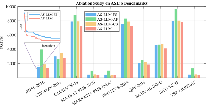
Figure 2: Ablation study on ASLib benchmarks.

To investigate the performance improvements brought by the key modules in AS-LLM, we conduct ablation experiments in this section, including AS-LLM-AF, AS-LLM-FS, and AS-LLM-CS. AS-LLM-AF removes the algorithm feature computation module from AS-LLM, relying solely on problem features for algorithm selection. AS-LLM-FS eliminates the feature selection process in AS-LLM to assess its impact on the model. AS-LLM-CS excludes the cosine similarity calculation module, using only MLP to derive the final results from the algorithm and problem representations. The results of the ablation experiments are presented in Figure 2.

The findings from Figure 2 reveal that, except for the CSP-MZN-013 scenario, AS-LLM outperforms all comparative methods, indicating the positive effects of the tested modules on the model. Notably, AS-LLM-AF exhibits the largest performance loss, underscoring the crucial role of algorithm features in algorithm selection and validating the core innovation of this study. In the CSP-MZN-013 scenario, the superiority of AS-LLM-AF over AS-LLM can be attributed to the unreliability of the algorithm feature source, specifically the inadequate representation of algorithm features in algorithm description texts. This highlights the dependence of AS-LLM on reliable algorithm data, preferably in the form of code files for all candidate algorithms. Additionally, besides demonstrating the performance loss of AS-LLM-FS compared to AS-LLM, the subplot in the top-left corner of Figure 2 showcases an example of the decreasing loss curves during training epochs for both approaches. This indicates that the feature selection module not only enhances algorithm selection performance but also facilitates easier and faster model convergence. The observed performance loss of AS-LLM-CS indicates the utility of the cosine distance computation, particularly when there is no requirement for generalizing the model to new candidate algorithms. Although the theoretical analyses have not explicitly demonstrated the cosine distance’s effectiveness, this empirical result highlights its practical value. Overall, the ablation experiments underscore the necessity of incorporating algorithm features and the utility of each module within AS-LLM.

5.4 More Experiments (Refer to Appendix C, D)

(1) Performance Comparison among Different Types of Algorithm Features: In Appendix C, we further compare algorithm features automatically extracted by LLM with manually-extracted features Pulatov et al. (2022), including 9 code features, 66 AST features, and their combination (75 features). The results demonstrate that the features extracted by LLM consistently outperform other feature types.

(2) Performance of Generalization over Algorithms: In Appendix D, we validate the generalization capacity over algorithms, which is a significant superiority conferred by the algorithm features. We individually exclude each candidate algorithm from the training data and observe the PAR10 score changes on the test set, which includes instances involving the excluded candidate algorithms. Results show that the generalized PAR10 scores do not significantly deviate from the performance obtained when training on all candidate algorithms, which demonstrates the generalization capability of AS-LLM_g over algorithms.

6 Conclusion

This paper explores the importance of algorithm features and their utilization in algorithm selection tasks. Specifically, the proposed AS-LLM leverages the powerful representation capabilities of LLMs to extract algorithm features from text related to code, representing a novel application of LLMs in this context. Additionally, AS-LLM incorporates a feature selection module to identify critical features and utilizes the similarity between algorithm and problem representations for algorithm selection. AS-LLM provides more refined modeling of the bidirectional relationship between algorithms and problems, demonstrating robust performance advantages in diverse scenarios. This paper not only emphasizes the potential of algorithm features to enhance algorithm generalization but also provides a rigorous theoretical upper bound to measure the generalization error in cases where both problems and algorithms undergo distribution shifts in the test set. Through its theoretical and methodological contributions, we firmly believe that the AS-LLM holds significant application potential in algorithm selection tasks.

References

- Abdulrahman et al. [2018] Salisu Mamman Abdulrahman, Pavel Brazdil, Jan N van Rijn, and Joaquin Vanschoren. Speeding up algorithm selection using average ranking and active testing by introducing runtime. Machine learning, 107:79–108, 2018.
- Amadini et al. [2014] Roberto Amadini, Maurizio Gabbrielli, and Jacopo Mauro. Sunny: a lazy portfolio approach for constraint solving. Theory and Practice of Logic Programming, 14(4-5):509–524, 2014.
- Bischl et al. [2016] Bernd Bischl, Pascal Kerschke, Lars Kotthoff, Marius Lindauer, Yuri Malitsky, Alexandre Fréchette, Holger Hoos, Frank Hutter, Kevin Leyton-Brown, Kevin Tierney, et al. Aslib: A benchmark library for algorithm selection. Artificial Intelligence, 237:41–58, 2016.
- Chen et al. [2021] Mark Chen, Jerry Tworek, Heewoo Jun, Qiming Yuan, Henrique Ponde de Oliveira Pinto, Jared Kaplan, Harri Edwards, Yuri Burda, Nicholas Joseph, Greg Brockman, et al. Evaluating large language models trained on code. arXiv preprint arXiv:2107.03374, 2021.
- Collautti et al. [2013] Marco Collautti, Yuri Malitsky, Deepak Mehta, and Barry OSullivan. Snnap: Solver-based nearest neighbor for algorithm portfolios. In Proceedings of the European Conference on Machine Learning and Knowledge Discovery in Databases, pages 435–450. Springer, 2013.
- Cunha et al. [2018] Tiago Cunha, Carlos Soares, and André CPLF de Carvalho. A label ranking approach for selecting rankings of collaborative filtering algorithms. In Proceedings of the 33rd Annual ACM Symposium on Applied Computing, pages 1393–1395, 2018.
- Fehring et al. [2022] Lukass Fehring, Jonas Manuel Hanselle, and Alexander Tornede. Harris: Hybrid ranking and regression forests for algorithm selection. In NeurIPS 2022 Workshop on Meta-Learning (MetaLearn 2022), 2022.
- Feng et al. [2020] Zhangyin Feng, Daya Guo, Duyu Tang, Nan Duan, Xiaocheng Feng, Ming Gong, Linjun Shou, Bing Qin, Ting Liu, Daxin Jiang, et al. Codebert: A pre-trained model for programming and natural languages. arXiv preprint arXiv:2002.08155, 2020.
- Floridi and Chiriatti [2020] Luciano Floridi and Massimo Chiriatti. Gpt-3: Its nature, scope, limits, and consequences. Minds and Machines, 30:681–694, 2020.
- Fusi et al. [2018] Nicolo Fusi, Rishit Sheth, and Melih Elibol. Probabilistic matrix factorization for automated machine learning. Proceedings of the Advances Conference in Neural Information Processing Systems, 31, 2018.
- Guo et al. [2020] Daya Guo, Shuo Ren, Shuai Lu, Zhangyin Feng, Duyu Tang, LIU Shujie, Long Zhou, Nan Duan, Alexey Svyatkovskiy, Shengyu Fu, et al. Graphcodebert: Pre-training code representations with data flow. In Proceedings of the 8th International Conference on Learning Representations, 2020.
- Guo et al. [2022] Daya Guo, Shuai Lu, Nan Duan, Yanlin Wang, Ming Zhou, and Jian Yin. Unixcoder: Unified cross-modal pre-training for code representation. In Proceedings of the 60th Annual Meeting of the Association for Computational Linguistics (Volume 1: Long Papers), pages 7212–7225, 2022.
- Hanselle [2020] Jonas Hanselle. Hybrid ranking and regression for algorithm selection. In German Conference on Artificial Intelligence, pages 59–72. Springer, 2020.
- Hansen and Ostermeier [2001] Nikolaus Hansen and Andreas Ostermeier. Completely derandomized self-adaptation in evolution strategies. Evolutionary Computation, 9(2):159–195, 2001.
- Heins et al. [2023] Jonathan Heins, Jakob Bossek, Janina Pohl, Moritz Seiler, Heike Trautmann, and Pascal Kerschke. A study on the effects of normalized tsp features for automated algorithm selection. Theoretical Computer Science, 940:123–145, 2023.
- Hilario et al. [2009] Melanie Hilario, Alexandros Kalousis, Phong Nguyen, and Adam Woznica. A data mining ontology for algorithm selection and meta-mining. In Proceedings of the ECML/PKDD09 Workshop on 3rd generation Data Mining (SoKD-09), pages 76–87. Citeseer, 2009.
- Hough and Williams [2006] Patricia Diane Hough and Pamela J Williams. Modern machine learning for automatic optimization algorithm selection. Technical report, Sandia National Lab.(SNL-CA), Livermore, CA (United States), 2006.
- Jang et al. [2016] Eric Jang, Shixiang Gu, and Ben Poole. Categorical reparameterization with gumbel-softmax. In Proceedings of the International Conference on Learning Representations, 2016.
- Kadioglu et al. [2010] Serdar Kadioglu, Yuri Malitsky, Meinolf Sellmann, and Kevin Tierney. Isac–instance-specific algorithm configuration. In Proceedings of the 19th European Conference on Artificial Intelligence, pages 751–756. IOS Press, 2010.
- Kerschke et al. [2019] Pascal Kerschke, Holger H Hoos, Frank Neumann, and Heike Trautmann. Automated algorithm selection: Survey and perspectives. Evolutionary Computation, 27(1):3–45, 2019.
- Koltchinskii [2001] Vladimir Koltchinskii. Rademacher penalties and structural risk minimization. IEEE Transactions on Information Theory, 47(5):1902–1914, 2001.
- Mısır and Sebag [2017] Mustafa Mısır and Michèle Sebag. Alors: An algorithm recommender system. Artificial Intelligence, 244:291–314, 2017.
- Nobel et al. [2021] Jacob Nobel, Hao Wang, and Thomas Baeck. Explorative data analysis of time series based algorithm features of cma-es variants. In Proceedings of the Genetic and Evolutionary Computation Conference, pages 510–518, 2021.
- Ouyang et al. [2022] Long Ouyang, Jeffrey Wu, Xu Jiang, Diogo Almeida, Carroll Wainwright, Pamela Mishkin, Chong Zhang, Sandhini Agarwal, Katarina Slama, Alex Ray, et al. Training language models to follow instructions with human feedback. Proceedings of the 35th Annual Conference on Advances in Neural Information Processing Systems, 35:27730–27744, 2022.
- Pio et al. [2023] Pedro B Pio, Adriano Rivolli, André CPLF de Carvalho, and Luís PF Garcia. A review on preprocessing algorithm selection with meta-learning. Knowledge and Information Systems, pages 1–28, 2023.
- Pulatov et al. [2022] Damir Pulatov, Marie Anastacio, Lars Kotthoff, and Holger Hoos. Opening the black box: Automated software analysis for algorithm selection. In Proceedings of the International Conference on Automated Machine Learning, pages 6–1. PMLR, 2022.
- Rice [1976] John R Rice. The algorithm selection problem. In Advances in Computers, volume 15, pages 65–118. Elsevier, 1976.
- Ruhkopf et al. [2022] Tim Ruhkopf, Aditya Mohan, Difan Deng, Alexander Tornede, Frank Hutter, and Marius Lindauer. Masif: Meta-learned algorithm selection using implicit fidelity information. Transactions on Machine Learning Research, 2022.
- Tornede et al. [2020] Alexander Tornede, Marcel Wever, and Eyke Hüllermeier. Extreme algorithm selection with dyadic feature representation. In Proceedings of the International Conference on Discovery Science, pages 309–324. Springer, 2020.
- Tornede et al. [2023] Alexander Tornede, Difan Deng, Theresa Eimer, Joseph Giovanelli, Aditya Mohan, Tim Ruhkopf, Sarah Segel, Daphne Theodorakopoulos, Tanja Tornede, Henning Wachsmuth, et al. Automl in the age of large language models: Current challenges, future opportunities and risks. arXiv preprint arXiv:2306.08107, 2023.
- Xiao et al. [2023] Shitao Xiao, Zheng Liu, Peitian Zhang, and Niklas Muennighof. C-pack: Packaged resources to advance general chinese embedding. arXiv preprint arXiv:2309.07597, 2023.
- Xu et al. [2008] Lin Xu, Frank Hutter, Holger H Hoos, and Kevin Leyton-Brown. Satzilla: portfolio-based algorithm selection for sat. Journal of Artificial Intelligence Research, 32:565–606, 2008.
- Xu et al. [2011] Lin Xu, Frank Hutter, Holger H Hoos, and Kevin Leyton-Brown. Hydra-mip: Automated algorithm configuration and selection for mixed integer programming. In Proceedings of Workshop at the 32nd International Joint Conference on Artificial Intelligence, pages 16–30, 2011.