$\mathtt{ComPEFT}$: Compression for Communicating Parameter Efficient Updates via Sparsification and Quantization

Abstract

Parameter-efficient fine-tuning (PEFT) techniques make it possible to efficiently adapt a language model to create “expert” models that specialize to new tasks or domains. Recent techniques in model merging and compositional generalization leverage these expert models by dynamically composing modules to improve zero/few-shot generalization. Despite the efficiency of PEFT methods, the size of expert models can make it onerous to retrieve expert models per query over high-latency networks like the Internet or serve multiple experts on a single GPU. To address these issues, we present $\mathtt{ComPEFT}$, a novel method for compressing fine-tuning residuals (task vectors) of PEFT-based models. $\mathtt{ComPEFT}$ employs sparsification and ternary quantization to reduce the size of the PEFT module without performing any additional retraining while preserving or enhancing model performance. In extensive evaluation across $\mathtt{T5}$, $\mathtt{T0}$, and $\mathtt{LLaMA}$-based models with $\mathtt{200M-65B}$ parameters, $\mathtt{ComPEFT}$ achieves compression ratios of $\mathtt{8x-50x}$. In particular, we show that $\mathtt{ComPEFT}$ improves with scale – stronger models exhibit higher compressibility and better performance. For example, we show $\mathtt{ComPEFT}$ applied to LLaMA outperforms QLoRA by $\mathtt{4.16}\%$ on MMLU with a storage size reduction of up to $\mathtt{26x}$. In addition, we show that the compressed experts produced by $\mathtt{ComPEFT}$ maintain few-shot compositional generalization capabilities, facilitate efficient communication and computation, and exhibit enhanced performance when merged. Lastly, we provide an analysis of different method components, compare it with other PEFT methods, and test $\mathtt{ComPEFT}$’s efficacy for compressing the residual of full-finetuning.

1 Introduction

Figure 1: $\mathtt{ComPEFT}$ improves performance with larger base models while compressing models significantly. Left Axis: Improvement of MMLU performance over the corresponding base model. Right Axis: Compression factor achieved by $\mathtt{ComPEFT}$ compared to the original checkpoint.

Figure 2: Left: ComPEFT can dramatically decrease communication costs when merging experts for compositional generalization. Right: $\mathtt{ComPEFT}$ employs ternary compression via sparsification and quantization to reduce the size of the PEFT module, while preserving or enhancing model performance, and without necessitating any additional training.

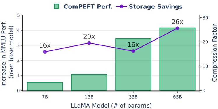
Parameter-efficient fine-tuning (PEFT) methods (Houlsby et al., 2019; Karimi Mahabadi et al., 2021; Lester et al., 2021) such as LoRA (Hu et al., 2021) and (IA)³ (Liu et al., 2022), facilitate the efficient adaptation of language models by learning a minimal set of new parameters. Notably, the recent QLoRA (Dettmers et al., 2023) method significantly reduces the memory requirements for adaptation by learning LoRA modules on top of a 4-bit quantized base model. This allows QLoRA to adapt base models with up to $\mathtt{65B}$ parameters on a single $\mathtt{48GB}$ GPU. Consequently, platforms like the like the Hugging Face model hub (Wolf et al., 2019) host an ever-growing number of specialized models (Luo et al., 2023a, b; Patil et al., 2023) that leverage PEFT methods for tasks related to multimodal understanding (Zhang et al., 2023), multilingual transfer (Yang et al., 2023), tool utilization (Patil et al., 2023), and domain-specific expertise like on math (Luo et al., 2023a), coding (Luo et al., 2023b), and beyond.

Recent works on model merging (Yadav et al., 2023; Choshen et al., 2022; Ilharco et al., 2023) and compositional generalization (Huang et al., 2023; Ponti et al., 2023; Caccia et al., 2022) have focused on leveraging the modularity of these expert models. These recent works enhance generalization to unseen domains and tasks by dynamically composing different expert PEFT models based on a given query or target dataset (Huang et al., 2023). This modular approach is a cost-effective and flexible solution for developing more sustainable NLP systems amid the rapid growth of resource-intensive machine learning models.

However, retrieving multiple experts for each query on the fly can be extremely slow over high-latency networks like the Internet. For example, the QLoRA adapter for the LLaMA-$\mathtt{65B}$ model is $\mathtt{3.2~{}GB}$ in size (comparable to the size of a full T5-Large model (Raffel et al., 2020a), which is $\mathtt{3.0~{}GB}$). Therefore, even if we have an effective method for model merging and composition generalization to unseen domains, retrieving even a handful of expert models could incur prohibitively high communication costs over high-latency networks (see Figure 2 (Left)).

To address these communication costs, we introduce $\mathtt{ComPEFT}$ method that compresses fine-tuning residuals (task vectors, i.e. the difference of the parameter values between the finetuned and the pre-trained checkpoints) by exploiting the value distribution within the task vector. Specifically, $\mathtt{ComPEFT}$ performs an initial sparsification to reset most values in the task vector to zero, followed by quantization, where the magnitude of remaining values is replaced by a single scalar constant. $\mathtt{ComPEFT}$ shares similarities with the Sparse Ternary Compression (STC, Sattler et al., 2019a) method used in federated learning; however, there are notable differences. Unlike STC, $\mathtt{ComPEFT}$ retains high-performance post-hoc compression without the need for additional training. While performance degradation is observed when using STC compression on the task vector, $\mathtt{ComPEFT}$ can restore full performance or even surpass the original performance by simply adjusting the constant value used for the magnitude of the ternary vector. Moreover, we find that the constant value magnitude for large models ($\mathtt{\geq 13B}$) is consistent for large models and does not need explicit tuning. Lastly, sparse ternary compression enables more efficient operations on task vectors that can e.g. make it faster to merge models or compute their similarity.

We perform comprehensive experiments for $\mathtt{ComPEFT}$ to evaluate: (1) the performance of the compressed model on its original tasks, (2) the number of bits needed to store the models, (3) the mergeability and composability of the compressed checkpoints, and (4) how $\mathtt{ComPEFT}$ compares to other existing PEFT methods. We performed experiments with $\mathtt{T5}$ (Raffel et al., 2020a), $\mathtt{T0}$ (Sanh et al., 2021a), and $\mathtt{LLaMA}$ (Touvron et al., 2023) as the base models with model sizes ranging from $\mathtt{200M-65B}$ parameters. We found that in most cases $\mathtt{ComPEFT}$ can provide compression of $\mathtt{8x-50x}$ (compared to $\mathtt{16-bit}$ precision PEFT checkpoints) while performing similarly or better than the uncompressed models. Notably, we found that as the base model gets bigger, their task vectors start to become more compressible and these compressed checkpoints significantly outperform the original uncompressed checkpoints. Specifically, as shown in Figure 1, $\mathtt{ComPEFT}$ leads to an improvement of $\mathtt{0.54}\%$, $\mathtt{1.06}\%$, $\mathtt{3.44}\%$, and $\mathtt{4.16}\%$ on MMLU for QLoRA trained on LLaMA $\mathtt{7B}$, $\mathtt{13B}$, $\mathtt{33B}$, and $\mathtt{65B}$ parameter models, respectively, while achieving $\mathtt{16x}-\mathtt{26x}$ compression in the model size.

Moreover, we find that the compressed models from $\mathtt{ComPEFT}$ lead to better-merged models and outperform strong baselines like Task Arithmetic (Ilharco et al., 2023) and TIES-Merging (Yadav et al., 2023) in $\mathtt{9/12}$ settings and lead to an improvement of $\mathtt{1.4}\%$ on average across all these settings. For few-shot compositional generalization, we adopt the experimental setting of LoraHub (Huang et al., 2023) and find that our compressed models lead to similar performance as the original models when evaluating on Big-Bench-Hard benchmark (Suzgun et al., 2022) for compositional generalization. In addition, we show (1) that $\mathtt{ComPEFT}$ applied to LoRA and (IA)³ is Pareto-optimal in terms of storage costs vs. performance compared to a wide range of existing, (2) the importance of the components of $\mathtt{ComPEFT}$ in an ablation study, and (3) the effect of sparsity and scaling on performance. Our results and analysis establish $\mathtt{ComPEFT}$ as an effective method for compressing task vectors to facilitate efficient communication for compositional generalization while also improving the performance that improves with model scale.

2 Background and Motivation

2.1 Problem Setting

Given a pre-trained model like $\mathtt{LLaMA}$ (Touvron et al., 2023) or $\mathtt{T5}$ (Raffel et al., 2020b) we can create an expert model for specific task $t$ by either finetuning all model parameters or using a parameter-efficient fine-tuning (PEFT) approach such as (IA)³ (Liu et al., 2022) or LoRA (Hu et al., 2021). In both scenarios, we represent the trainable parameters as $\theta$, initialized as $\theta_{\mathtt{init}}$, which, upon fine-tuning, become $\theta_{\mathtt{ft}}$. This work assumes access to the initial model parameters $\theta_{\mathtt{init}}$ and the fine-tuned model parameters, $\theta_{\mathtt{ft}}$, and focuses on (1) compressing parameter updates for efficient communication to enable fast transfer over high-latency networks like the internet, and (2) understanding the intrinsic dimensionality of parameter updates. These updates are formulated as task vectors $\tau\in\mathbb{R}^{\textrm{d}}$ (Ilharco et al., 2023), which are expressed as $\tau=\theta_{\mathtt{ft}}-\theta_{\mathtt{init}}$ and encapsulate the “knowledge” learned in the fine-tuning phase. Our work delves into the characteristics of task vectors and introduces a compression method, $\mathtt{ComPEFT}$. Our overarching objective is facilitating a repository containing thousands or millions of cheaply communicable expert models to bolster the prospects of fast retrieval of expert models for zero/few-shot compositional generalization (Caccia et al., 2022; Ponti et al., 2023; Huang et al., 2023) and model merging (Yadav et al., 2023; Ilharco et al., 2023).

2.2 Motivation

Many past works have shown that task vectors can be compressed by adopting various techniques like (1) sparsification (Yadav et al., 2023; Sattler et al., 2019a; Sung et al., 2021) – removing some parameters that are not crucial for the performance; or (2) quantization (Dettmers et al., 2023; Sattler et al., 2019a) – reducing the number of bits that represent each parameter. These are two complementary ways to reduce the amount of information stored, reducing the number of nonzero entries in the task vector, and reducing the amount of information in each of each entry. Next, we discuss both of these approaches while focusing on compressing task vectors as opposed to full model weights.

Sparsity of the Learnt Updates.

The task vectors, $\tau_{\mathtt{t}}=\theta_{\mathtt{ft}}-\theta_{\mathtt{init}}$, denote the aggregate changes to each parameter during the model finetuning phase. Past works (Yadav et al., 2023) have shown that for any given task, $\mathtt{70-90}\%$ of the values in the task vector can be pruned without hurting the performance of the tasks. Presumably, this is true because most parameters have small changes and only accumulate noisy gradient updates. In Appendix A.3 we analyze and find that most parameters indeed changed very little during finetuning. Hence, sparsity can act as an important tool for compressing task vectors.

Quantizing the Parameter Updates.

Many works (Dettmers et al., 2023; Sattler et al., 2019b) employ post-training quantization to reduce the number of bits needed to represent each parameter. They perform compression by using lower precision datatypes for storing model weights and performing computation. For example, converting a checkpoint from 32-bit floating points to 8-bit integers can result in $\mathtt{4x}$ reduction in memory (Liang et al., 2021b).

In this work, we employ both sparsification and quantization to compress our parameter updates from $\mathtt{16}$- or $\mathtt{32}$-bit floating point values to a sparse ternary vector, i.e. a sign vector with values $\in\{-1,0,+1\}$ and a single scalar constant. This massively reduces the storage requirements and communication costs.

3 $\mathtt{ComPEFT}$: Compression for Communicating Parameter Efficient Updates via Sparsification and Quantization

Following the success of the above-mentioned methods, we now present we present $\mathtt{ComPEFT}$, which uses sparsification and quantization to heavily compress task vectors in order to address the aforementioned issues of communicating parameter updates over high-latency networks for compositional generalization.

Input: Task vector $\tau_{\mathtt{t}}$, $k$, and a scaling value $\alpha$.

Output: Compressed task vector $\tilde{\tau}_{\mathtt{t}}$

$\triangleright$ Step 1: Decompose.

$\gamma_{\mathtt{t}}\leftarrow sgn(\tau_{\mathtt{t}})$

$\mu_{\mathtt{t}}\leftarrow|\tau_{\mathtt{t}}|$

$\triangleright$ Step 2: Sparsify.

$\tilde{\tau}_{\mathtt{t}}\leftarrow\text{keep\_topk\_reset\_rest\_to\_zero}(\gamma_{\mathtt{t}},\mu_{\mathtt{t}},k)$

$\triangleright$ Step 3: Quantize Magnitudes to scalar.

$\tilde{\tau}_{\mathtt{t}}=\alpha*\sigma(\tau_{\mathtt{t}})*\tilde{\gamma}_{\mathtt{t}}$

return $\tilde{\tau}_{\mathtt{t}}$

Algorithm 1 $\mathtt{ComPEFT}$ Compression Procedure.

3.1 Preliminaries

The task vector $\tau_{\mathtt{t}}=\theta_{\mathtt{ft}}-\theta_{\mathtt{init}}$ for a particular task $t$ encapsulates the changes to the parameter values that occur after fine-tuning on the task. We can deconstruct the task vector $\tau_{\mathtt{t}}$ into two distinct vectors: a direction (sign) vector $\gamma_{\mathtt{t}}\in\mathbb{R}^{d}$ and a magnitude vector $\mu_{\mathtt{t}}\in\mathbb{R}^{d}$. Formally, $\gamma_{\mathtt{t}}=\text{sgn}(\tau_{\mathtt{t}})$, where the signum function $\text{sgn}(x)$satisfies the condition $\text{sgn}(x)\cdot|x|=x$ and outputs values of $\mathtt{+1}$, $\mathtt{0}$ or $\mathtt{-1}$ based on the sign of $x$. The magnitude vector $\mu_{\mathtt{t}}$ is computed as $\mu_{\mathtt{t}}=|\tau_{\mathtt{t}}|$. Finally, we can decompose $\tau_{\mathtt{t}}$ as the Hadamard product (element-wise multiplication) of these vectors by$\tau_{\mathtt{t}}=\gamma_{\mathtt{t}}\odot\mu_{\mathtt{t}}$. $\mathtt{ComPEFT}$ performs extreme compression of the task vectors by sparsifying the sign vector $\gamma_{\mathtt{t}}$ by up to $95\%$ and compressing the $d$-dimensional magnitude vector $\mu_{\mathtt{t}}\in\mathbb{R}^{d}$ to a single scalar value.

3.2 Steps in $\mathtt{ComPEFT}$

To reconstruct an expert model for task $t$, we only need to communicate the update over the base pre-trained model which is denoted by the task vector $\tau_{\mathtt{t}}$. Given this task vector, $\mathtt{ComPEFT}$ follows three simple steps for compression (see Algorithm 1 and Figure 2):

1. Decompose: For each task $t$, we create the task vector, $\tau_{\mathtt{t}}=\theta_{\mathtt{ft}}-\theta_{\mathtt{init}}$ and decompose it into a direction vector $\gamma_{\mathtt{t}}\in\mathbb{R}^{d}$ and a magnitude vector $\mu_{\mathtt{t}}\in\mathbb{R}^{d}$ such that $\tau_{\mathtt{t}}=\gamma_{\mathtt{t}}\odot\mu_{\mathtt{t}}$.

2. Sparsify: We sparsify the sign vector $\gamma_{\mathtt{t}}$ to keep only the parameters (or their indices) corresponding to the top-$k$ values based on their magnitude and set the sign for the $(1-k)$ smallest-magnitude parameters to $0$. Formally, the sparsified direction vector, $\tilde{\gamma}_{\mathtt{t}}=\gamma_{\mathtt{t}}\odot\mathtt{top-k}(\mu_{\mathtt{t}})$, where $\mathtt{top-k}(.)$ is applied elementwise and returns $\mathtt{True}$ for indices with the $\mathtt{top-k}$ magnitude values $\mathtt{False}$ otherwise. Hence, we refer to the parameter $k$ as the “density” and refer to the sparsity as $1-k$.

3. Quantize Magnitudes: Lastly, we propose to replace the magnitude vector $\mu_{\mathtt{t}}\in\mathbb{R}^{d}$ with a single scalar constant. Specifically, we define the final compressed task vector $\tilde{\tau}_{\mathtt{t}}$ as $\tilde{\tau}_{\mathtt{t}}=\alpha*\sigma(\tau_{\mathtt{t}})*\tilde{\gamma}_{\mathtt{t}}$, where $\sigma(\tau_{\mathtt{t}})$ is the standard deviation of the original task vector $\tau_{\mathtt{t}}$ and $\alpha$ is a scaling constant. The value of $\alpha$ is selected by evaluating a metric of choice on a small validation set. We find that scaling $\alpha$ is enough to mitigate any performance loss that happens due to sparsification and ternarization (in contrast with most model pruning methods that perform additional retraining after sparsification to recover performance).

3.3 Efficient Storage of $\mathtt{ComPEFT}$ Models

Entropy of the Sparsified Task Vector.

Typically, a given task vector $\tau_{\mathtt{t}}$ is stored in a 16-bit float format ($\mathrm{bfloat16}$ or $\mathrm{fp16}$) and therefore requires $\mathtt{16*d~{}bits}$ to store on disk. If values in $\tau_{\mathtt{t}}$ are uniformly distributed, the entropy of the update is also $\mathbb{H}_{\mathtt{dense}}=16*d~{}\mathtt{bits}$. On the other hand, our compressed $\tilde{\tau}_{\mathtt{t}}$ is a combination of a sparse ternary sign vector with values $\in\{-1,0,+1\}$ and a $16$-bit scalar value $\alpha*\sigma(\tau_{\mathtt{t}})\in\mathbb{R}$. Hence, assuming the signs of the nonzero entries of $\tilde{\tau}_{\mathtt{t}}$ are uniformly distributed, the ternarization step reduces the entropy of the update to $\mathbb{H}_{\mathtt{ComPEFT}}=-((1-k)\log_{2}(1-k)+k\log_{2}(\frac{k}{2}))*d+16~{}\mathtt{bits}$, where $k$ is the density of the update. At a density level of $k=0.05$, the resultant update has $95\%$ of the values as $0$ and the entropy is $0.34*d+16~{}\mathtt{bits}$. Hence, with a perfect encoding-decoding scheme and 95% sparsity, our $\mathtt{ComPEFT}$ can reduce the number of bits per parameter from $16~{}\mathtt{bits}$ to approximately $0.34~{}\mathtt{bits}$ which is a $47\mathtt{x}$ improvement in communication and storage requirements. Next, we talk about two ways to store and communicate the compressed models.

Optimal Compression: Communicating Distances using Golomb Code.

To communicate $\tilde{\tau}_{\mathtt{t}}$, we can transfer the locations of non-zero elements with an additional bit indicating each element’s sign. If the weight updates have a random sparsity pattern then the distances between non-zero entries are geometrically distributed with success probability $p$ equal to the sparsity, i.e., one minus the density, $p=1-k$. Hence, similar to past works (Strom, 2015; Sattler et al., 2019a, b), we can use the Golomb code (Golomb, 1966) to optimally encode the distances to reduce the average number of position bits to

$$\bar{\texttt{b}}_{pos}=\mathbf{b}^{*}+\frac{1}{1-(1-p)^{2^{\mathbf{b}^{*}}}},$$ (1)

with $\mathbf{b}^{*}=1+\lfloor\log_{2}(\frac{\log(\phi-1)}{\log(1-p)})\rfloor$ and $\phi=\frac{\sqrt{5}+1}{2}$ being the golden ratio. This scheme in total needs $-((1-k)\log_{2}(1-k)+k\log_{2}(\frac{k}{2}))*d+16~{}\mathtt{bits}$ to store the compressed checkpoint. Unless specified otherwise, we report the storage cost when using Golomb Code in all of our experiments.

$\mathtt{ModelSize}$ ($\rightarrow$)	$\mathtt{7B}$		$\mathtt{13B}$		$\mathtt{33B}$		$\mathtt{65B}$
$\mathtt{Dataset}$ ($\downarrow$)	$\mathtt{Original}$	$\mathtt{ComPEFT}$	$\mathtt{Original}$	$\mathtt{ComPEFT}$	$\mathtt{Original}$	$\mathtt{ComPEFT}$	$\mathtt{Original}$	$\mathtt{ComPEFT}$
$\mathtt{LLaMA~{}no~{}tuning}$	35.1	-	46.9	-	57.8	-	63.4	-
$\mathtt{Self-Instruct}$	36.45(0.3)	37.72(0.03)	36.20(0.47)	45.15(0.01)	50.98(0.91)	57.02(0.02)	55.34(1.49)	63.43(0.03)
$\mathtt{Longform}$	34.37(0.3)	35.48(0.02)	45.70(0.47)	46.80(0.02)	54.60(0.91)	57.07(0.07)	59.49(1.49)	62.95(0.05)
$\mathtt{Chip2}$	34.88(0.3)	36.11(0.02)	44.19(0.47)	45.06(0.03)	51.72(0.91)	56.43(0.03)	57.30(1.49)	63.32(0.05)
$\mathtt{HH-RLHF}$	35.52(0.3)	35.30(0.01)	44.66(0.47)	44.99(0.01)	53.41(0.91)	56.97(0.07)	58.79(1.49)	63.42(0.05)
$\mathtt{UnnaturalInstruct}$	42.14(0.3)	41.82(0.02)	48.98(0.47)	48.42(0.03)	56.65(0.91)	58.07(0.09)	59.50(1.49)	63.30(0.03)
$\mathtt{Guanaco(OASST1)}$	35.02(0.3)	36.31(0.01)	48.50(0.47)	47.10(0.03)	55.51(0.91)	57.55(0.05)	60.67(1.49)	63.25(0.09)
$\mathtt{Alpaca}$	40.72(0.3)	39.95(0.02)	49.53(0.47)	48.41(0.03)	53.66(0.91)	57.68(0.05)	60.51(1.49)	63.28(0.05)
$\mathtt{FLANv2}$	43.97(0.3)	44.70(0.02)	50.45(0.47)	50.76(0.03)	56.67(0.91)	60.01(0.07)	62.72(1.49)	64.61(0.11)
$\mathtt{Average}$	37.88(0.3)	38.42(0.0188)	46.03(0.47)	47.09(0.024)	54.15(0.91)	57.60(0.056)	59.29(1.49)	63.45(0.058)
$\mathtt{Improvement/Compression}$	$-$	+0.54 / $\mathtt{16x}$	$-$	+1.06 / $\mathtt{20x}$	$-$	+3.44 / $\mathtt{16x}$	$-$	+4.16 / $\mathtt{26x}$

Table 1: Performance improvement from $\mathtt{ComPEFT}$ increases as models get bigger. We present the performance (storage size in GB) on the MMLU Test for the original and compressed QLoRA models. For $\mathtt{LLaMA-65B}$, $\mathtt{ComPEFT}$ leads to a $\mathtt{4.16\%}$ improvement while being $\mathtt{26x}$ smaller.

Efficient Computation and Communication via Two Binary Vectors. The compressed task vector $\tilde{\tau}_{\mathtt{t}}$ can also be stored as two binary masks, one signifying positive values and the other signifying negative values. Formally, we need to communicate $\tilde{\tau}_{\mathtt{t}}^{+}=(\tilde{\tau}_{\mathtt{t}}$ == $+1)\in\mathbb{R}^{d}$ and $\tilde{\tau}_{\mathtt{t}}^{-}=(\tilde{\tau}_{\mathtt{t}}$ == $-1)\in\mathbb{R}^{d}$, and the scalar constant $\alpha*\sigma(\tau_{\mathtt{t}})$. Each binary mask needs $\mathtt{1~{}bit/parameter}$, resulting in $\mathtt{2*d+16~{}bits}$ for communicating the update. Note that this requires strictly more storage than the Golomb-based encoding described above because $-((1-k)\log_{2}(1-k)+k\log_{2}(\frac{k}{2}))<2$. However, sparse ternary vectors allow for efficient matrix operations. For example, to efficiently compute the distance between $\tilde{\tau}_{\mathtt{t_{1}}}$ and $\tilde{\tau}_{\mathtt{t_{2}}}$, we can do an $\mathtt{XOR}$ ($\oplus$) followed by a $\mathtt{POPCNT}$ for each group of 64 parameters (i.e. two machine instructions on a 64-bit architecture) twice, once for the positive and once for the negative masks. The dot product can also be calculated by using bitwise $\mathtt{AND}$ operations to calculate positive contributions (both vectors have $+1$ or $-1$) and negative contributions (one vector has $+1$, the other $-1$). The final dot product is the difference between the sum of these contributions. Similarly, other operations such as addition can also be made faster, which could reduce the time when merging models.

4 Main Results

In our main experiments, we show that even parameter-efficient finetuning task vectors exhibit remarkably low intrinsic dimensionality, namely, most of their parameters are unnecessary. This finding enables substantial compression with better or similar performance on downstream tasks (§ 4.1,4.2,4.5). These efficiently compressed task vectors can be transmitted cheaply over high-latency networks, facilitating both model merging and compositional generalization for novel tasks (§ 4.3,4.4). Importantly, as model size and zero-shot abilities increase, the compressibility and the performance of $\mathtt{ComPEFT}$ also increase (§ 4.1).

4.1 Compressing QLoRA Trained on LLaMA Models

Experimental Setup.

We first explore the utility of $\mathtt{ComPEFT}$ in the setting of training QLoRA adapters (Dettmers et al., 2023) for the $\mathtt{LLaMA}$ models (Touvron et al., 2023) with $\mathtt{7B}$, $\mathtt{13B}$, $\mathtt{33B}$, and $\mathtt{65B}$ parameters. We follow the experimental setting from the QLoRA paper (Dettmers et al., 2023) and experiment with $\mathtt{8}$ recent instruction-following datasets that are diverse in terms of languages and dataset sizes. This collection includes datasets generated by language models (Alpaca (Taori et al., 2023), self-instruct (Wang et al., 2022), and unnatural-instructions (Honovich et al., 2022)), a multitask dataset (FLAN-v2 (Chung et al., 2022a)), two datasets created via human annotation and feedback (OASST1 (Köpf et al., 2023) and HH-RLHF (Bai et al., 2022)), and two hybrid datasets (Chip2 (LAION, 2023) and Longform (Köksal et al., 2023)). For each of these datasets, we reuse the checkpoints released as part of the QLoRA paper to perform compression using Algorithm 1 and then evaluate the 5-shot performance of the compressed QLoRA module on the MMLU benchmark (Hendrycks et al., 2020). In all experiments, we sweep both $\alpha$ and $k$ in the following ranges, $k\in\{5,10,20,30,50\}$ and $\alpha\in\{0.5,1,2,3,4,5,6,8,10\}$ and report the storage size based on the entropy of $\mathtt{ComPEFT}$ as specified in §3.3. We find that at any given value of $k$, you can achieve good performance (see § 5.2). We used a single 48GB NVIDIA A6000 GPU for these experiments.

Outcomes.

In Table 1, we provide results for all the task and model size combinations, comparing the performance of the $\mathtt{ComPEFT}$ checkpoints and the original QLoRA checkpoints along with (in subscripts) the storage size in GB assuming 16-bit precision for uncompressed models and Golomb code-based compression for compressed models. We find that on $\mathtt{28}$ of $\mathtt{32}$ experimental configurations $\mathtt{ComPEFT}$ improves upon the performance of the original QLoRA models while compressing the LoRA module between $\mathtt{10x}-\mathtt{50x}$ in terms of storage costs. $\mathtt{ComPEFT}$ leads to an improvement of $\mathtt{0.54}\%$, $\mathtt{1.06}\%$, $\mathtt{3.44}\%$, and $\mathtt{4.16}\%$ on MMLU for the $\mathtt{LLaMA}$ $\mathtt{7B}$, $\mathtt{13B}$, $\mathtt{33B}$, and $\mathtt{65B}$ parameter models, respectively. To sum, $\mathtt{ComPEFT}$ provides better results while also reducing the QLoRA module size. For example, on the $\mathtt{65B}$ $\mathtt{LLaMA}$ base model it reduces the storage size from $\mathtt{1.5}$GB to $\mathtt{110}$MB while improving the MMLU performance by a large margin of $4.16\%$.

Discussion.

A few important conclusions about $\mathtt{ComPEFT}$ can be derived from these results: (1) $\mathtt{ComPEFT}$ can compress all QLoRA models by a factor of at least $\mathtt{10x}$. (2) Larger base models allow for more compressible LoRA modules. We get a compression factor of approximately $\mathtt{16x}$, $\mathtt{20x}$, $\mathtt{16x}$, and $\mathtt{26x}$ for $\mathtt{7B}$, $\mathtt{13B}$, $\mathtt{33B}$, and $\mathtt{65B}$ parameter models respectively. (3) A similar trend is found in performance – the performance gap between the original and the compressed LoRA module increases with model size from $\mathtt{0.54}\%$ for the $\mathtt{7B}$ model to $\mathtt{4.16}\%$ for the $\mathtt{65B}$ model. If this scaling law continues, it means that the utility of methods like $\mathtt{ComPEFT}$ will increase as models become larger and/or their zero-shot performance improves.

$\mathtt{PEFT}$ ($\downarrow$)	$\mathtt{Method}$ ($\downarrow$)	$\mathtt{T5-Base}$	$\mathtt{T5-Large}$	$\mathtt{T0-3B}$
(IA)3	Original	81.3(0.25)	86.2(0.66)	89.3(1.03)
	$\mathtt{ComPEFT}$	80.0(0.01)	85.9(0.04)	88.4(0.06)
	Improvement	-1.3 / $\mathtt{25x}$	-0.3 / $\mathtt{16x}$	-0.9 / $\mathtt{17x}$
LoRA	Original	79.2(6.19)	84.5(16.50)	89.5(33.75)
	$\mathtt{ComPEFT}$	78.1(0.35)	84.6(1.37)	89.5(2.60)
	Improvement	-1.1 / $\mathtt{17x}$	+0.1 / $\mathtt{12x}$	0.0 / $\mathtt{13x}$

Table 2: $\mathtt{ComPEFT}$ can compress smaller model with minimal performance loss. Test set performance${}_{\text{(Storage Size in MB)}}$ averaged over seven GLUE tasks when compressing (IA)³ and LoRA modules on different base models.

4.2 Compressing PEFT Updates

The finding that scaling the base model makes the PEFT modules more compressible and more performant brings up the question as to whether $\mathtt{ComPEFT}$ is still effective at smaller scales. We perform experiments on two widely used PEFT methods, (IA)³ (Liu et al., 2022) and LoRA (Hu et al., 2021), with three models, T5-Base and T5-Large (Raffel et al., 2020a), and T0-3B (Sanh et al., 2021b). Specifically, we compress (IA)³ and LoRA modules trained on $\mathtt{7}$ classification tasks from the GLUE benchmark (Wang et al., 2018a) belonging to three categories: Natural Language Inference (MNLI (Williams et al., 2018), RTE (Bentivogli et al., 2009), QNLI (Rajpurkar et al., 2016), WNLI (Levesque et al., 2012a)), Sentiment Analysis (SST2 (Socher et al., 2013)), and Paraphrase Detection (MRPC (Dolan & Brockett, 2005), QQP (Wang et al., 2018a)).

Outcomes.

In Table 2, we present the average performance on the $\mathtt{7}$ aforementioned GLUE tasks (per-dataset results are provided in Appendix B.3) along with the average checkpoint size in MB (in subscripts) for three base models with both (IA)³ and LoRA adapters. We find that even with smaller base models, $\mathtt{ComPEFT}$ compress the PEFT modules by a factor of $\mathtt{12x-25x}$ with minimal to no loss in performance. These results demonstrate that even at smaller scales $\mathtt{ComPEFT}$ can lead to substantial compression. Additionally, we performed some experiments with BERT (Devlin et al., 2018), RoBERTa (Liu et al., 2019a), and T5v1.1 (Raffel et al., 2020a) models that are not multitask-trained and/or have poor zero-shot performance (i.e. they generally require additional finetuning to perform well on any downstream tasks). We present the results for these models in Appendix B.4, where we observe that compression works well for LoRA with minimal performance loss. However, for (IA)³ we observe significant performance drops which suggest that zero-shot performance may be important to enable $\mathtt{ComPEFT}$ compression of (IA)³-based models.

$\mathtt{Method}$ ($\downarrow$)	$\mathtt{T5-Base}$		$\mathtt{T5-Large}$		$\mathtt{T0-3B}$
	$\mathtt{(IA)^{3}}$	$\mathtt{LoRA}$	$\mathtt{(IA)^{3}}$	$\mathtt{LoRA}$	$\mathtt{(IA)^{3}}$	$\mathtt{LoRA}$
$\mathtt{Averaging}$	53.7	49.3	55.4	50.2	74.5	73.1
$\mathtt{TaskArithmetic~{}(TA)}$	60.0	52.8	62.7	61.6	77.8	75.0
$\mathtt{ComPEFT}$ $\mathtt{~{}+~{}TA}$	59.7	53.9	61.9	64.9	80.0	75.6
$\mathtt{TIES-Merging}$	55.5	49.2	61.3	57.3	71.7	73.4
$\mathtt{ComPEFT}$ $\mathtt{~{}+~{}TIES}$	55.6	49.2	60.4	61.4	76.2	75.8

Table 3: $\mathtt{ComPEFT}$ compressed checkpoints lead to better merged models. Average test set results on $\mathtt{7}$ GLUE tasks when employing different merging methods on the original uncompressed checkpoints and the compressed $\mathtt{ComPEFT}$ checkpoints.

4.3 Merging Compressed PEFT Modules

Experimental Setup.

Next, we examine the effectiveness of $\mathtt{ComPEFT}$ when merging models (Choshen et al., 2022; Matena & Raffel, 2021; Wortsman et al., 2022a) by comparing the merging of compressed or uncompressed models. We follow the experimental setting (including base models, PEFT methods, and datasets) from the previous section and merge the $\mathtt{7}$ GLUE tasks to produce a multitask model. We then report the average performance of the merged across all tasks. We use two methods to merge task vectors, namely, Task Arithmetic (Ilharco et al., 2023) and TIES-Merging (Yadav et al., 2023). We used the code from the original authors for both merging methods.

Outcomes.

As demonstrated in Table 3, in $\mathtt{9}$ out of $\mathtt{12}$ scenarios, the $\mathtt{ComPEFT}$ checkpoints lead to better merged models compared to the original checkpoints, with the notable exception of (IA)³ on T5 models. Notably, in stronger models like T0-3B, $\mathtt{ComPEFT}$-compressed checkpoints not only reduce the size by approximately $\mathtt{15x}$ but also improve the merged model’s performance by $\mathtt{2.4}\%$ on average. This shows $\mathtt{ComPEFT}$’s efficacy in both minimizing storage and communication overheads and improving the model merging performance.

Figure 3: $\mathtt{ComPEFT}$ facilitates compositional generalization. Average performance of LoraHub and $\mathtt{ComPEFT}$ for compositional generalization on Big-Bench-Hard.

4.4 Cross-Task Generalization via Dynamic LoRA Module Composition

Experimental Setup.

Next, we assess the impact of $\mathtt{ComPEFT}$ compression on the composability of the resulting PEFT modules for cross-task generalization. Specifically, given a set of expert models and an unseen downstream task with few training examples, the goal is to combine a subset of these expert modules to attain a model that performs well on the unseen task.

For this, we follow the LoraHub (Huang et al., 2023) method and their experimental setting. We use the Flan-T5-large (Chung et al., 2022b) model as it exhibits strong zero-shot and few-shot capabilities. We consider nearly $200$ distinct (tasks, instruction) pairs that were utilized to train the Flan-T5 model and use the LoRA modules trained on these tasks as expert candidates. Following LoraHub (Huang et al., 2023), when learning a new unseen task, we randomly select $\mathtt{N}$ LoRA modules denoted by $\{L_{i}=(A_{i},B_{i})\}_{i=1}^{N}$ and compose them as

$$L_{m}=A_{m}B_{m}=\left(\sum_{i=1}^{N}w_{i}A_{i}\right)\left(\sum_{i=1}^{N}w_{i}B_{i}\right),$$ (2)

where $A_{m}$, $B_{m}$ are the matrics of the composed LoRA module and $w_{i}$ are parameters that are learned on the few-shot examples from the unseen tasks using the gradient-free Shiwa optimizer (Liu et al., 2020). Following LoraHub, we use $\mathtt{N}=20$ and treat the $\mathtt{27}$ diverse tasks from the Big-Bench Hard (BBH) benchmark (Suzgun et al., 2022) as our unseen evaluation tasks. All the tasks are multiple-choice questions and we employ Exact Match (EM) as our evaluation metric.

Outcomes.

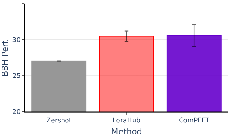
In Figure 3, we report the average performance over 5 seeds along with the standard deviation obtained when using the LoraHub method on the original checkpoints and the $\mathtt{ComPEFT}$-compressed checkpoints. We find that the $\mathtt{ComPEFT}$-compressed checkpoints exhibit similar compositional abilities as the original uncompressed checkpoints. Hence, we claim that $\mathtt{ComPEFT}$ checkpoints can be communicated quickly over high latency networks while maintaining their compositional abilities.

Figure 4: $\mathtt{ComPEFT}$ are Pareto-optimal. Performance vs storage size for multiple PEFT methods averaged over $\mathtt{11}$ tasks. A PEFT method is Pareto-optimal if it attains better performance (higher on the y-axis) than all methods that use less storage space (to the left on the x-axis). In particular, $\mathtt{Com(IA)^{3}}$ performance is comparable to PEFT methods that require $\mathtt{1000\times}$ more storage space.

4.5 Comparision of $\mathtt{ComPEFT}$ with Other PEFT Methods

Experimental Setup.

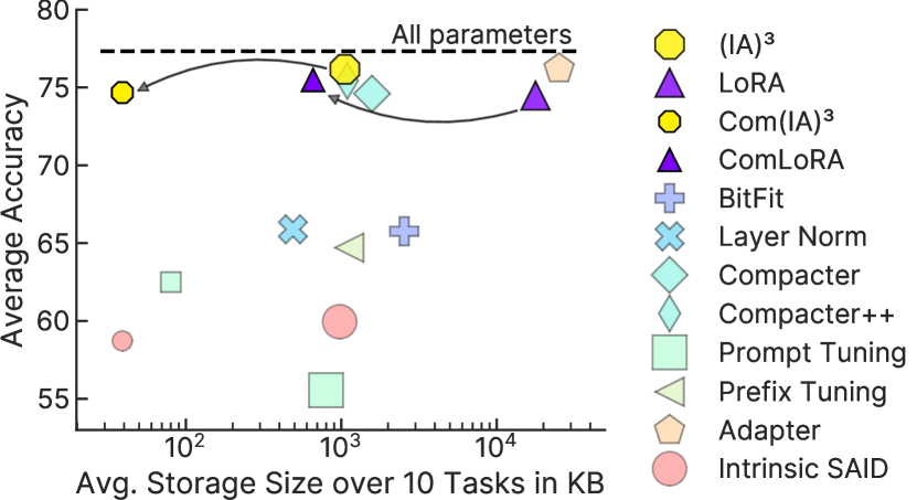
Next, we compare the (IA)³ and LoRA checkpoints compressed by $\mathtt{ComPEFT}$ with various other PEFT methods to determine whether $\mathtt{ComPEFT}$ produces Pareto-optimal parameter-efficient fine-tuning in terms of Storage Size and Performance. For this, we use the T0-3B (Sanh et al., 2021b) model and train a wide range of PEFT methods on the $\mathtt{11}$ held-out datasets from Sanh et al. (2021b) – specifically, sentence completion (COPA (Roemmele et al., 2011), H-SWAG (Zellers et al., 2019), and Story Cloze (Sharma et al., 2018) datasets), natural language inference (three splits of ANLI (Nie et al., 2019), CB (Marneffe et al., 2019), and RTE (Dagan et al., 2005)), coreference resolution (WSC (Levesque et al., 2012b) and Winogrande (Sakaguchi et al., 2020)), and word sense disambiguation (WiC (Pilehvar & Camacho-Collados, 2019)). For each task, from the training set, we select $\mathtt{200}$ example for the validation set and then use the first template from Prompt Source (Bach et al., 2022) both during training and evaluation. We perform experiments with $\mathtt{10}$ different PEFT methods from Liu et al. (2022) – LoRA (Hu et al., 2021), (IA)³ (Liu et al., 2022), BitFit (Zaken et al., 2021), LayerNorm, Adapters (Houlsby et al., 2019), Compacter and Compactor++ (Karimi Mahabadi et al., 2021), Prompt Tuning (Lester et al., 2021), Prefix Tuning (Li & Liang, 2021), and Intrinsic SAID (Aghajanyan et al., 2020).

(a) T0-3B

(b) LLaMA-7B

(c) LLaMA-13B

(d) LLaMA-33B

(e) LLaMA-65B

Figure 5: $\mathtt{ComPEFT}$ outperforms STC and all method steps are crucial. Average performance as density $\mathtt{k}$ of the compressed checkpoint increases. We show results for compressing LoRA modules trained over different models with sizes ranging from $\mathtt{3B-65B}$ and compare them with baselines and ablate method components.

Outcomes.

In Figure 4, we plot the average performance over the $\mathtt{11}$ tasks and the checkpoint sizes in KB for $\mathtt{10}$ PEFT Method and when using $\mathtt{ComPEFT}$ on LoRA and (IA)³ checkpoints, i.e. $\mathtt{ComLoRA}$ and $\mathtt{Com(IA)^{3}}$. We find that $\mathtt{ComPEFT}$ reduces the storage size for both LoRA and (IA)³ by more than an order of magnitude with minimal reduction in performance. From this plot, $\mathtt{ComPEFT}$ is Pareto-optimal, i.e. for any given storage budget, $\mathtt{ComPEFT}$ outperforms all other PEFT methods. Notably, $\mathtt{Com(IA)^{3}}$ exhibits only a minor performance degradation compared to full-model fine-tuning while being one of the most space-efficient PEFT methods. Lastly, we note that for $\mathtt{ComPEFT}$ you can trade-off performance for storage cost by varying the density $k$ to obtain models of different storage sizes. Hence, $\mathtt{Com(IA)^{3}}$ and $\mathtt{ComLoRA}$ could be made even more space efficient.

5 Additional Results and Analysis

5.1 Ablation of $\mathtt{ComPEFT}$ Components

Experimental Setup.

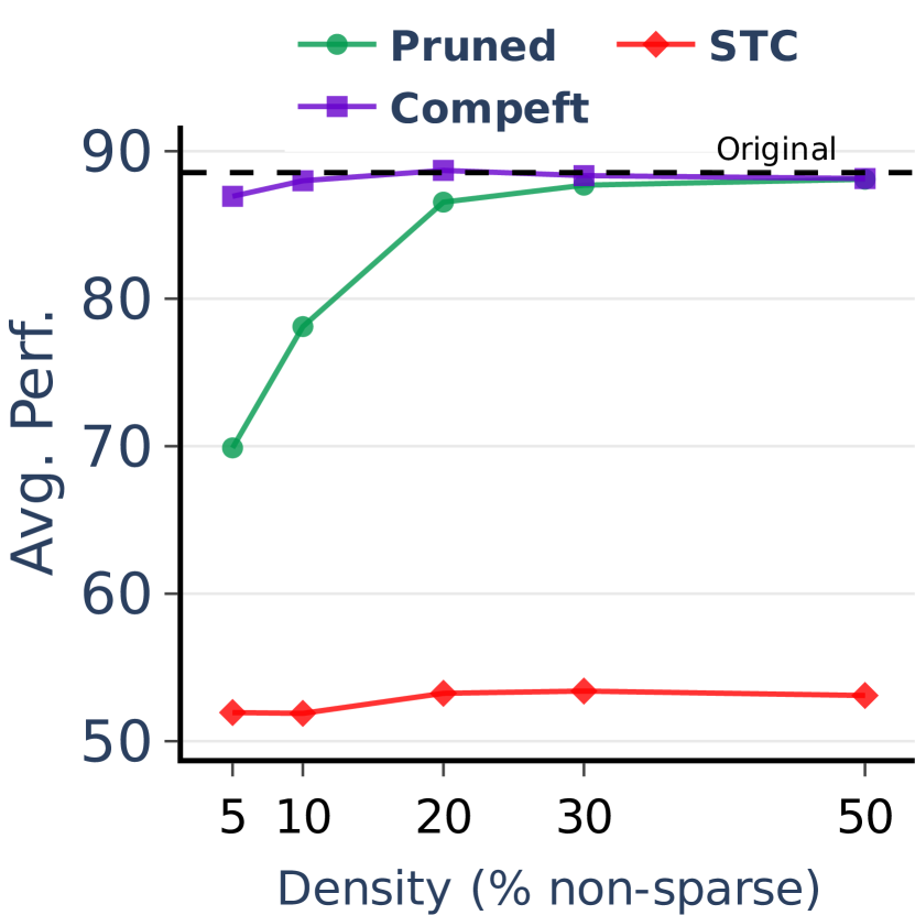
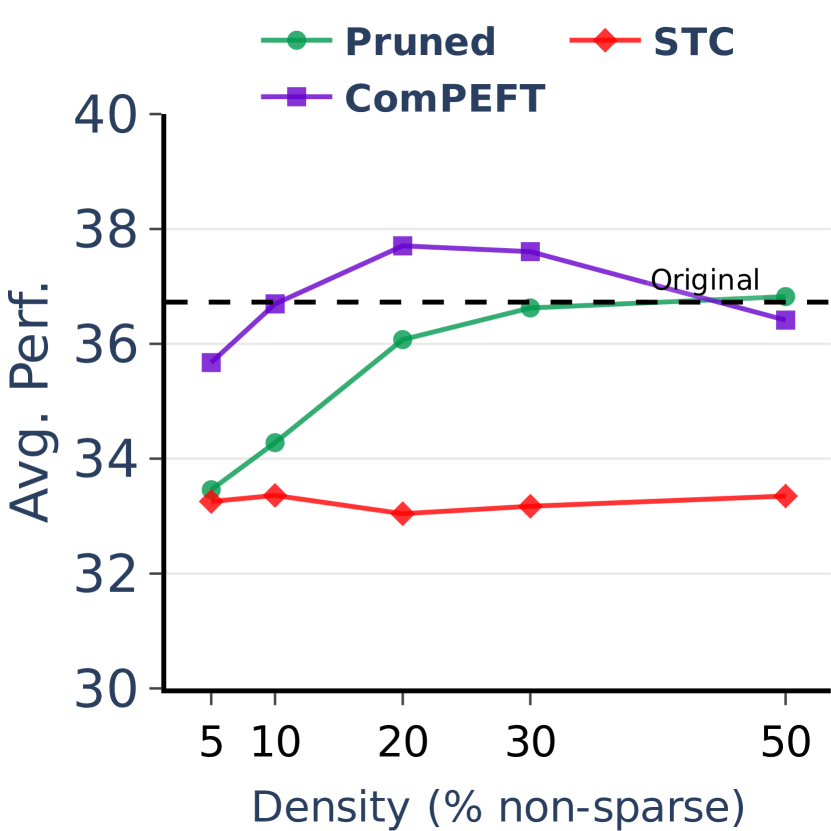
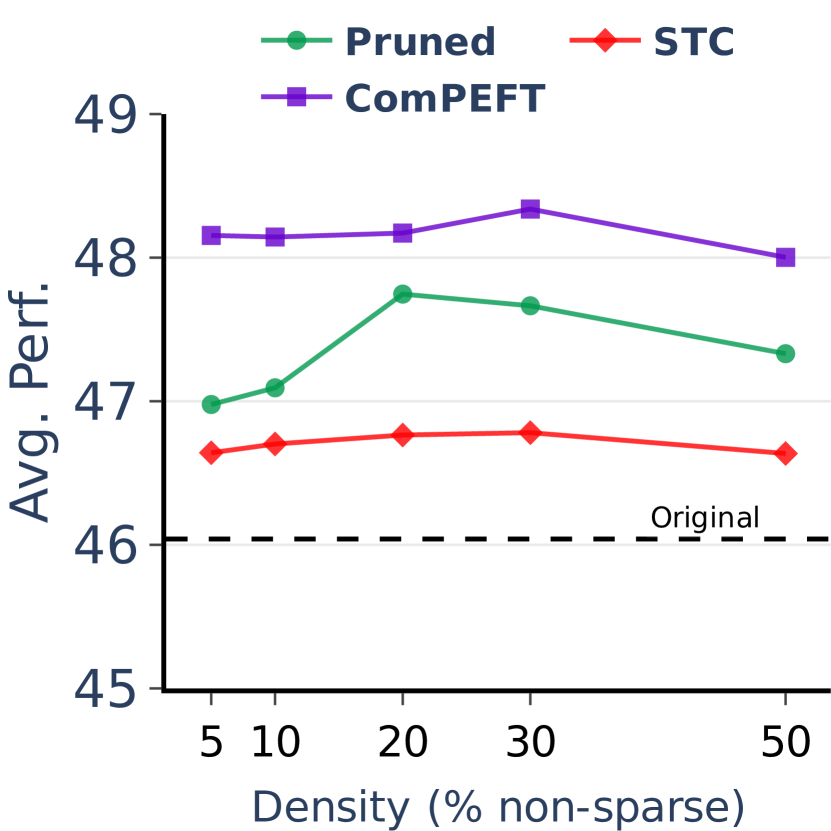
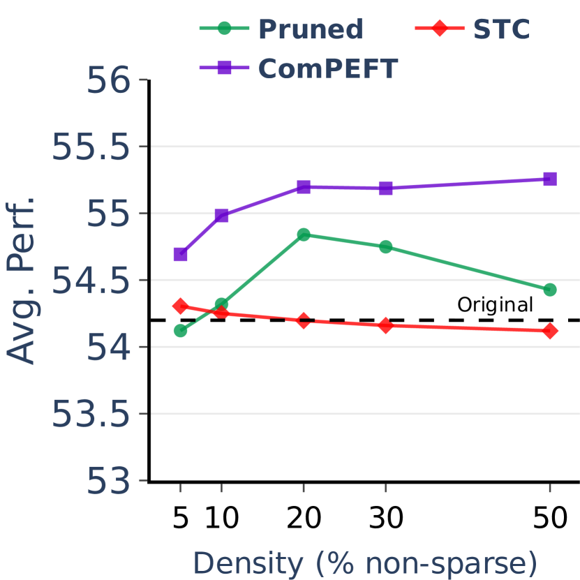
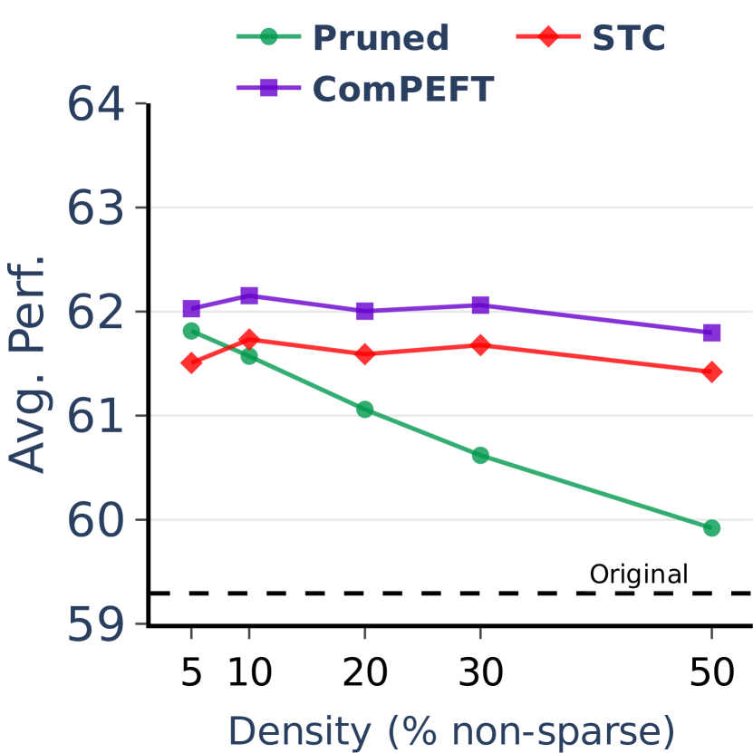
To understand the contribution of the individual steps of $\mathtt{ComPEFT}$, we now perform a brief ablation study. In $\mathtt{ComPEFT}$ there are two main steps: (1) Pruning the task vectors, and (2) Converting the pruned task vector to a ternary vector and scaling to find the optimal $\alpha$ value. Hence, we compare with two ablated versions, i.e. the unpruned original model, and Pruned variant where we reset values in the task vector but do not perform the ternarization step. We also compare with Sparse Ternary Compression (STC) (Sattler et al., 2019a) as it also performs ternary compression but sets the magnitude of the ternary vector as the mean magnitude of the pruned task vector as opposed to tuning $\alpha*\sigma(\tau_{\mathtt{t}})$ for $\mathtt{ComPEFT}$. We provide these ablations for the experimental settings from § 4.1 and 4.5 where the model sizes range from $\mathtt{3B-65B}$.

Outcomes.

In Figure 5, we plot the average validation set performance over tasks as a function of the density ($k$) of the pruned model. From these results, we make a few observations: (1) $\mathtt{ComPEFT}$ almost always performs better than both STC and the Pruned version for all model sizes and sparsity levels. (2) $\mathtt{ComPEFT}$ almost always performs better than or similar to the original model’s performance for all sparsity levels. In contrast, for smaller model sizes of $\mathtt{3B}$ and $\mathtt{7B}$, STC’s performance is much worse than the original models. This highlights the importance of the scaling $\alpha$ as proposed in $\mathtt{ComPEFT}$, which allows us to recover the performance lost due to pruning and ternary compression without any additional retraining. (3) At low density, the performance of Pruned is much worse than $\mathtt{ComPEFT}$ and this gap reduces as the density increases. However, note that the size of $\mathtt{ComPEFT}$ is much smaller than the Pruned baseline due to ternarization. (4) At larger base model sizes ($\geq\mathtt{13B}$), all the methods at all density levels perform similarly to or better than the original LoRA checkpoint. This suggests that at larger scales PEFT modules are much more robust to the exact choice of hyperparameters.

(a) T0-3B

(b) LLaMA-7B

(c) LLaMA-13B

(d) LLaMA-33B

(e) LLaMA-65B

Figure 6: Larger models do not require explicit tuning of $\alpha$. Performance vs $\alpha$ for various denisty levels for $\mathtt{ComPEFT}$.

5.2 Effect of Sparsity and Scaling on $\mathtt{ComPEFT}$ Performance

Experimental Setup.

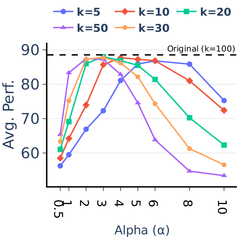
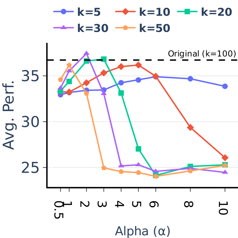
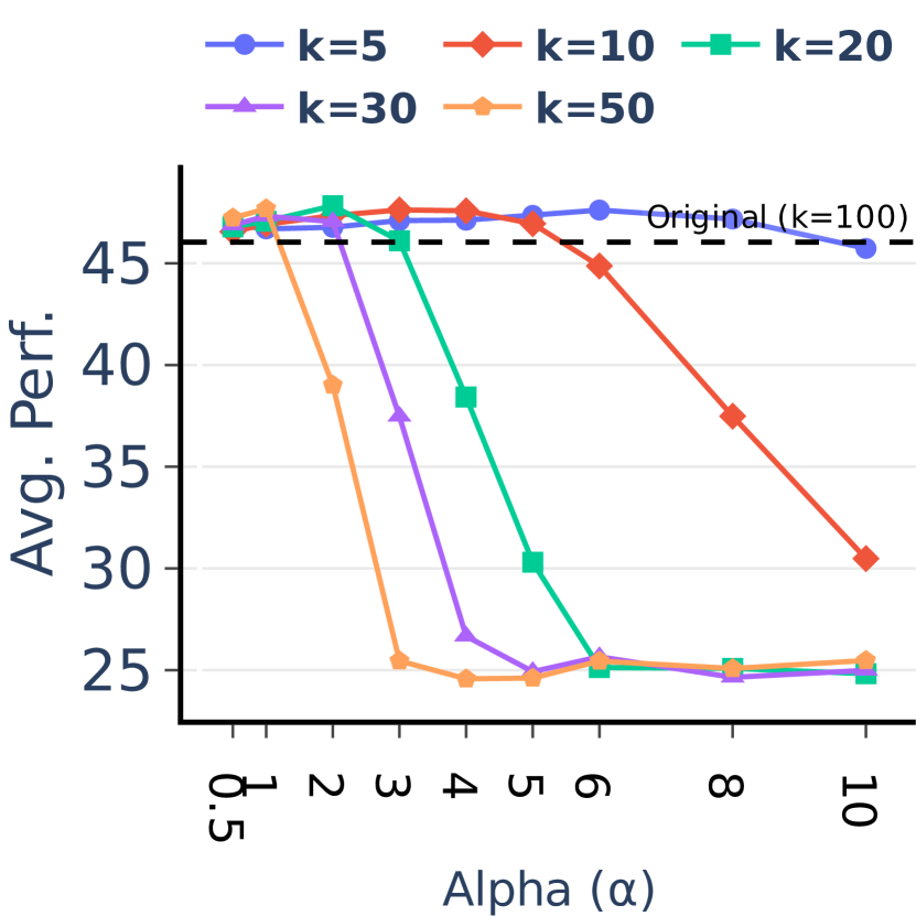
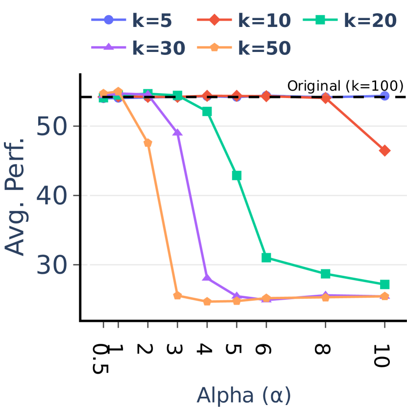
For $\mathtt{ComPEFT}$, we analyze the effect of different levels of sparsity and the scaling value $\alpha$ on the performance of the compressed checkpoints. We present this analysis for $\mathtt{T0-3B}$ and $\mathtt{LLaMA}$ as the base models; the experimental settings are similar to § 4.1 and 4.5 where the model sizes range from $\mathtt{3B-65B}$. We provide results for different values of the density $k$ (sparsity = $100-k$), specifically, the values $k\in\{5,10,20,30,50\}$ and different values of $\alpha\in\{0.5,1,2,3,4,5,6,8,10\}$.

Outcomes.

In Figure 6, we plot the average validation set performance across all tasks with respect to the scaling coefficient $\alpha$. We make the following observations; (1) For smaller base-model sizes ($\mathtt{3B}$ and $\mathtt{7B}$) and across density values, we find a similar trend – as the value of $\alpha$ increases, the average validation performance first increases and then drops. (2) As the value of $k$ increases, the optimal value of $\alpha$ becomes smaller. For example, for the T0-3B base model, the optimal value $\alpha$ for $k=50$ is between $\mathtt{2-3}$ while for $k=5$ the optimal $\alpha$ is in the range $\mathtt{5-8}$. (3) For bigger base-models ($\mathtt{\geq 13B}$) and low density ($k\in\{5,10,20\}$) the variation in performance as $\alpha$ changes is smaller. (4) Lastly, as the base-model size increases, smaller values of $\alpha\in(0.5,2)$ and a bigger range of values start to work better. Hence, for large models, the need for tuning $\alpha$ can be removed. For models with $\mathtt{\geq 13B}$ parameters and high sparsity $k\leq\mathtt{20}$, we recommend simply setting $\alpha=1$.

$\mathtt{Model}$ ($\downarrow$)	$\mathtt{Original}$	$\mathtt{ComPEFT}$	$\mathtt{Improvement}$
$\mathtt{BERT-Base}$	87.2(0.21)	86.8(0.011)	-0.4 / $\mathtt{19x}$
$\mathtt{BERT-Large}$	86.3(0.64)	86.1(0.036)	-0.2 / $\mathtt{18x}$
$\mathtt{RoBERTa-Base}$	85.5(0.24)	83.3(0.013)	-2.2 / $\mathtt{18x}$
$\mathtt{RoBERTa-Large}$	88.6(0.68)	89.2(0.052)	+0.6 / $\mathtt{13x}$
$\mathtt{T5v.1-Base}$	74.1(0.47)	75.8(0.032)	+1.7 / $\mathtt{15x}$
$\mathtt{T5v.1-Large}$	84.0(1.5)	82.2(0.11)	-1.8 / $\mathtt{14x}$
$\mathtt{T5-Base}$	82.8(0.43)	78.1(0.032)	-4.7 / $\mathtt{13x}$
$\mathtt{T5-Large}$	85.2(1.41)	84.7(0.12)	-0.5 / $\mathtt{12x}$

Table 4: $\mathtt{ComPEFT}$ can also compress full-model task vectors. Test set performance${}_{\text{(Storage Size in GB)}}$ averaged over seven GLUE tasks when compressing fully finetuned model’s task vectors.

5.3 Compressing Full Finetuning Updates

Experimental Setup.

In this experiment, we assess the usefulness of $\mathtt{ComPEFT}$ compression when compressing task vectors produced by full-model fine-tuning (i.e. not parameter-efficient fine-tuning). We adopt the experimental setting from § 4.2 to finetune the $\mathtt{7}$ classification tasks and then compress the finetuned model using $\mathtt{ComPEFT}$. We present results on four different models (BERT (Devlin et al., 2018), RoBERTa (Liu et al., 2019a), T5-v1.1 (Raffel et al., 2020a), and T5 (Raffel et al., 2020a)) and two different different sizes (Base and Large) for each of the model.

Outcomes.

In Table 4, we present the average test set performance over the $\mathtt{7}$ GLUE task. We observe that $\mathtt{ComPEFT}$ also performs well when compressing fully finetuned models leading $\mathtt{12x-19x}$ times smaller models with minimal loss in performance. Notably, for T5v1.1-base and RoBERTa-large models $\mathtt{ComPEFT}$ leads to $\mathtt{1.7}\%$ and $\mathtt{0.6}\%$ improvements while compressing the original model by $\mathtt{15x}$ and $\mathtt{13x}$ respectively. These results show that $\mathtt{ComPEFT}$ can also be used to compress fully finetuned models with minimal loss in performance.

6 Related Work

Paremeter Efficient Fine-Tuning.

Several parameter-efficient techniques have emerged as efficient alternatives to full fine-tuning in the field of pre-trained language models (PLMs). These methods, including Prompt Tuning (Lester et al., 2021), Prefix Tuning (Li & Liang, 2021), Adapters (Houlsby et al., 2019), and Compacter (Karimi Mahabadi et al., 2021), introduce a small number of additional parameters to PLMs (Raffel et al., 2020a; Touvron et al., 2023), enabling modularization and knowledge sharing. LoRA (Hu et al., 2021) incorporates trainable low-rank matrices into transformer layers, while BitFit (Zaken et al., 2021) focuses on updating bias terms. In Contrast, (IA)³ (Liu et al., 2022) learns a new set of parameters to rescale the model activations. Recently, QLoRA (Dettmers et al., 2023) proposed training LoRA modules over a $\mathtt{4-bit}$ quantized base model to further save the memory.

Network Pruning and Federated Learning.

With the increasing size of neural networks, network pruning techniques have garnered attention for reducing computational costs (Cheng et al., 2017; Liang et al., 2021a). Network pruning aims to remove redundant model parameters while preserving performance (Zhu & Gupta, 2018; Liu et al., 2019b; Frankle & Carbin, 2019; Gale et al., 2019; Xia et al., 2022). Among these, magnitude-based pruning (Han et al., 2015; Li et al., 2018; Lee et al., 2021) selects parameters based on magnitudes, while structured pruning techniques (McCarley et al., 2020; Wang et al., 2019; Kwon et al., 2022) prioritize inference speed at the cost of model performance. In federated learning, model pruning is valuable due to high communication costs over slow networks. Atomo (Wang et al., 2018b) minimizes gradient variance through unbiased sparsification, while QSGD (Alistarh et al., 2017) offers a communication-convergence trade-off by quantizing gradients. SignSGD (Bernstein et al., 2018) further converts gradients to binary sign vectors. TernGrad (Wen et al., 2017) and STC (Sattler et al., 2019a) combine sparsification and quantization techniques. Unlike most federated learning methods that assume many rounds of training, our proposed approach addresses communication challenges without further training.

Model Merging.

Various merging methods (Ortiz-Jiménez et al., 2023; Wortsman et al., 2022b, a; Ilharco et al., 2022; Ramé et al., 2022; Sung et al., 2023; Yu et al., 2023) aim to combine fine-tuned models for improved performance in various applications. (Choshen et al., 2022) perform direct averaging of the model weights, whereas RegMean (Jin et al., 2023) solves a linear regression problem for each linear layer but requires additional data statistics and inference steps. Fisher Merging (Matena & Raffel, 2021) uses the Fisher Information Matrix to weigh parameters in merging, while Task Arithmetic (Ilharco et al., 2023) generates task vectors and performs arithmetic operations to create multitask checkpoints. Ortiz-Jiménez et al. (2023) offer theoretical insights into model merging by using the weight disentanglement property and demonstrate that fine-tuning models within their tangent space improves this property, resulting in better model merging. TIES-Merging (Yadav et al., 2023) identifies the issue of parameter interference in model merging and tackles it by trimming low-magnitude parameters, resolving sign disagreements, and disjointly merging parameters with consistent signs.

Compositional Generalization.

Recent advancements in the field of multi-task learning have aimed to improve generalization across various tasks. FLAN (Wei et al., 2021), T0 (Sanh et al., 2021a), and InstructGPT (Ouyang et al., 2022) focus on enhancing the generalization capabilities of multi-task models. The CrossFit (Ye et al., 2021) framework requires minimal labeled data for few-shot fine-tuning but relies on task names as hard prefixes, limiting generalization. ReCross (Lin et al., 2022) reduces the need for labeled examples through retrieval but still involves a fine-tuning process. Ponti et al. (2023) jointly learn adapters and a routing function to allocate skills to tasks, while  Caccia et al. (2023) analyzes task routing for more efficient cross-task generalization. LoraHub (Huang et al., 2023) employs gradient-free optimization to retrieve and merge expert modules for unseen tasks. For an overview of PEFT methods, model merging, and compositional generalization, we refer to the comprehensive survey by Pfeiffer et al. (2023).

7 Conclusion

Our novel PEFT compression method, $\mathtt{ComPEFT}$, offers an effective solution to the latency challenges associated with retrieving expert models for parameter-efficient fine-tuning. By compressing fine-tuning residuals through sparsification and quantization, $\mathtt{ComPEFT}$ achieves high compression ratios and often enhances model performance across various NLP tasks and model sizes. Moreover, it preserves few-shot compositional generalization capabilities, facilitates efficient communication and computation, and demonstrates improved performance when merged with original models. This research contributes valuable insights into the realm of parameter-efficient fine-tuning, addressing both performance and latency concerns.

Appendix A Implementation Details

A.1 Training Details

In our research, we utilized the following models, BERT-base, BERT-Large, RoBERTa-base, RoBERTa-large, T5v1.1-base, T5v1.1-large, T5-base, T5-large, Flan-T5-large, T0-3B, LLaMA $\mathtt{7B,13B,33B,65B}$ models. The Flan-T5-Large and LLaMA models were not trained by us and were used by the authors of QLoRA (Dettmers et al., 2023) and LoraHub (Huang et al., 2023). For the experiments in §4.2 and §5.3 on the 7 GLUE (Wang et al., 2018a) tasks, we trained the large datasets (mnli, qnli, sst2, qqp) for 1 epoch and the small datasets (rte, mrpc, wnli) for 10 epochs. Whereas for the experiment in §4.5, we followed most of the hyperparameter configuration from the (IA)³ (Liu et al., 2022) paper and trained for 2500 steps with a batch size of 8. For each of the 11 datasets in §4.5, we selected 200 examples from the training set to be used as the validation set for best model selection as well as selecting the hyperparameters for $\mathtt{ComPEFT}$. Across all experiments to obtain the trained models we selected different learning rates for each dataset and PEFT method. For training (IA)³ models we selected the learning rate from $\{1e-2,1e-3,1e-4,1e-5\}$, for LoRA from $\{5e-2,5e-3,5e-4,5e-5\}$, and for full model finetuning from $\{5e-3,5e-4,5e-5,5e-6\}$. During the training process, bfloat16 was adopted to curtail GPU memory expenditure. For the purpose of evaluation, models from the T5 and T0 families were evaluated using rank classification to select the correct label. In this method, the model’s log probabilities for all potential label strings are ranked. The model’s prediction is deemed accurate if the choice ranked highest aligns with the correct answer. It should be noted that rank classification evaluation can accommodate both classification tasks and multiple-choice tasks.

A.2 Compute Resources Used and Runtimes

We executed all our experiments on Nvidia A6000 GPUs equipped with 48GB RAM. Training (IA)³ and LoRA models on the T0-3B model for a single (§4.2, §4.5, and §4.3) task takes about 30 minutes to 4 hours depending on the dataset. For T5-Base and T5-Large models (§4.2, §4.3), based on dataset size, needed between 15 minutes and 2 hours per task. Experiments with QLoRA on LLaMA models were done using the original checkpoints from QLoRA paper (Dettmers et al., 2023) for all the 8 instruction tuning datasets and are supplied the authors of QLoRA here. The $\mathtt{ComPEFT}$ compression experiments were efficient, with evaluations consuming between 10-30 seconds for the T5-Base, T5-Large, and T0-3B models. For LLaMA models, following QLoRA (Dettmers et al., 2023), the hyperparameter selection is done on a small held-out subset of MMLU (Hendrycks et al., 2020) benchmark and takes about 8 minutes, 14 minutes, 28 minutes, and 49 minutes for LLaMA $\mathtt{7B}$, $\mathtt{13B}$, $\mathtt{33B}$, and $\mathtt{65B}$ models respectively.

A.3 Gradient Noise

Gradients are (almost) never 0 for any parameter, as all parameters somehow affect the result. Thus, we presume most updates in fine-tuning are not more than just noise, rather than learned updates. We compute the mean and standard deviation of the task vector of a LoRA model finetuned on LLaMa (Touvron et al., 2023) base model and compare it with the base model. We find the mean of both the LoRA task vector and the base model is close to zero, however, the LoRA task vector has a small standard deviation of $\mathtt{0.0007}$ as compared to $\mathtt{0.0228}$ for the LLaMA base. This further confirms the hypothesis that most parameters are changed very little during fine-tuning.

Appendix B Additional Results

B.1 Validation Set Results

In Table 5 and 6, we provide the validation set results for our main compression experiments on $\mathtt{LLaMA,T5,T0}$ experiments from Section 4.1 and 4.2 respectively.

B.2 Full Results for Compositional Generalization

In Table 7, we present the Zeroshot, ICL, LoraHub, and $\mathtt{ComPEFT}$ results for each of the BBH tasks.

B.3 Individual Task Results

We present the task level validation and test set results along with model sizes of (IA)³, LoRA, and full finetuning for T5-base (Table 14), T5-large (Table 15), T0-3B (Table 16).

B.4 Compressing Model With Smaller Models with Bad ZeroShot Performance

We present the task level validation and test set results along with model sizes for (IA)³, LoRA, and full finetuning for BERT-base (Table 8), BERT-large (Table 9), RoBERTa-base (Table 10), RoBERTa-large (Table 11), T5-v1.1-base (Table 12), and T5-v1.1-large (Table 13). These models are only trained using the pretraining objective and are not multitask-trained. Hence, these models have very bad zero/few-shot performance and always require explicit finetuning to perform well on any downstream tasks. We observe that for the LoRA method, the performance of $\mathtt{ComPEFT}$ is similar to the uncompressed full models while being smaller in size. This hints at the fact that the intrinsic dimensionality of the LoRA adaptation is much smaller compared to the number of parameters in the LoRA module. However, for (IA)³ method, the performance drop is more, we believe that two reasons for this are: (1) The models are not good zero/few-shot models, and (2) (IA)³ adds very few parameters to perform a multiplicative operation on the activations. Therefore, the loss landscape is not as smooth as for good zershot models, and due to this IA3 has to scale different activations in a very different manner to learn the task. Hence, compressing (IA)³ to sparse sign-vector and a constant is not feasible. Whereas, In the case of Lora the updates are added and hence their impact on the final value of the parameter is not huge as the maximum of the LoRA parameter is still very small compared to the base model’s parameter value.

$\mathtt{Dataset}$ ($\downarrow$)	$\mathtt{ComPEFT}$
	$\mathtt{7B}$	$\mathtt{13B}$	$\mathtt{33B}$	$\mathtt{65B}$
Self-Instruct	35.62	47.52	55.11	62.13
Longform	31.89	47.80	55.31	62.27
Chip2	33.49	47.15	55.02	62.21
HH-RLHF	32.37	47.19	54.78	62.06
Unnatural Instruct	42.41	49.62	56.28	62.15
Guanaco	33.92	49.52	55.35	62.00
Alpaca	39.82	49.00	55.91	62.37
FLAN v2	43.93	50.86	56.97	63.77
Average	37.88	48.58	55.59	62.37

Table 5: We present the performance${}_{\text{(Storage Size in GB)}}$ on MMLU Validation for the compressed QLoRA models.

$\mathtt{Method}$ ($\downarrow$)	$\mathtt{T5-Base}$		$\mathtt{T5-Large}$		$\mathtt{T0-3B}$
	$\mathtt{(IA)^{3}}$	$\mathtt{LoRA}$	$\mathtt{(IA)^{3}}$	$\mathtt{LoRA}$	$\mathtt{(IA)^{3}}$	$\mathtt{LoRA}$
Original	81.25	81.94	85.08	86.21	87.71	89.94
$\mathtt{ComPEFT}$	81.04	80.96	85.28	86.54	89.14	89.95
Improvement	-0.21	-0.98	0.2	0.33	1.43	0.01

Table 6: Validation set performance${}_{\text{(Storage Size in MB)}}$ averaged over seven GLUE tasks when compressing (IA)³ and LoRA modules on different base models.

Table 7: Task level results: Average performance over 5 seed for LoraHub and $\mathtt{ComPEFT}$ for compositional generalization on Big-Bench-Hard.

Task	Zeroshot	ICL	LoraHub (Avg)	$\mathtt{ComPEFT}$ (Avg)	LoraHub (Best)	$\mathtt{ComPEFT}$ (Best)
Logical Deduction Three Objects	0.0	51.3	41.9	28.4	51.3	48.0
Tracking Shuffled Objects Five Objects	12.0	12.0	9.6	11.3	12.0	12.0
Web Of Lies	54.0	54.0	28.1	41.7	49.3	56.0
Tracking Shuffled Objects Seven Objects	6.7	6.7	5.3	6.7	6.7	6.7
Date Understanding	15.3	22.7	39.5	29.1	42.0	38.7
Navigate	47.3	44.0	48.4	38.5	50.7	50.0
Multistep Arithmetic Two	0.7	0.7	0.7	0.5	1.3	0.7
Boolean Expressions	54.0	58.7	55.9	55.7	57.3	61.3
Hyperbaton	6.7	74.0	55.2	49.9	65.3	67.3
Tracking Shuffled Objects Three Objects	24.7	30.7	26.7	21.6	29.3	24.7
Sports Understanding	56.0	56.0	46.4	53.1	54.7	58.0
Logical Deduction Seven Objects	12.7	42.0	35.5	37.6	40.0	40.0
Causal Judgement	57.5	56.3	40.7	49.2	58.6	57.5
Penguins In A Table	43.5	39.1	36.1	44.3	45.7	47.8
Geometric Shapes	6.7	18.7	9.6	7.3	19.3	9.3
Reasoning About Colored Objects	32.0	38.7	38.0	40.8	39.3	44.0
Dyck Languages	1.3	2.7	1.1	0.7	1.3	1.3
Disambiguation Qa	0.0	69.3	14.3	6.5	51.3	29.3
Salient Translation Error Detection	37.3	46.0	31.3	38.5	44.7	43.3
Movie Recommendation	62.7	52.7	61.1	58.0	67.3	62.0
Snarks	50.0	55.1	49.2	50.0	50.0	50.0
Formal Fallacies	51.3	58.0	41.3	41.1	52.7	51.3
Logical Deduction Five Objects	21.3	40.0	33.6	36.3	36.7	42.0
Temporal Sequences	16.7	26.7	18.7	19.5	20.0	21.3
Word Sorting	1.3	0.7	1.2	1.3	1.3	1.3
Ruin Names	23.3	18.7	18.0	22.4	23.3	23.3
Object Counting	34.7	32.0	35.5	35.3	36.7	36.0
Average	27.0	37.3	30.5	30.6	37.3	36.4

Table 8: Validation and Test set performance along with storage size in MB for bert-base-uncased Model, for (IA)³, LoRA and Full model finetuning.

		Original (Val)	Original (Test)	$\mathtt{ComPEFT}$ (Val)	$\mathtt{ComPEFT}$ (Test)
PEFT	Task
full	mnli	$84.7$	$83.1_{(208.8)}$	$84.3$	$82.6_{(12.0)}$
	mrpc	$86.8$	$97.5_{(208.8)}$	$86.8$	$97.0_{(19.6)}$
	qnli	$91.9$	$91.0_{(208.8)}$	$91.9$	$90.9_{(12.0)}$
	qqp	$90.1$	$90.3_{(208.8)}$	$90.0$	$90.0_{(15.4)}$
	rte	$66.4$	$94.5_{(208.8)}$	$69.0$	$94.0_{(7.4)}$
	sst2	$91.1$	$97.0_{(208.8)}$	$92.2$	$96.0_{(7.4)}$
	wnli	$56.3$	$57.0_{(208.8)}$	$56.3$	$57.0_{(4.4)}$
ia3	mnli	$79.2$	$78.9_{(0.1)}$	$57.6$	$56.2_{(0.0)}$
	mrpc	$84.6$	$94.5_{(0.1)}$	$31.6$	$34.5_{(0.0)}$
	qnli	$87.9$	$87.5_{(0.1)}$	$49.3$	$49.6_{(0.0)}$
	qqp	$84.6$	$84.4_{(0.1)}$	$63.2$	$63.2_{(0.0)}$
	rte	$59.2$	$73.5_{(0.1)}$	$52.7$	$55.5_{(0.0)}$
	sst2	$91.5$	$91.0_{(0.1)}$	$49.1$	$45.5_{(0.0)}$
	wnli	$54.9$	$57.0_{(0.1)}$	$56.3$	$57.0_{(0.0)}$
lora	mnli	$82.5$	$81.4_{(2.6)}$	$76.6$	$76.9_{(0.2)}$
	mrpc	$86.3$	$97.5_{(2.6)}$	$82.8$	$94.0_{(0.2)}$
	qnli	$91.7$	$91.0_{(2.6)}$	$90.8$	$90.1_{(0.2)}$
	qqp	$89.4$	$89.5_{(2.6)}$	$87.4$	$87.5_{(0.2)}$
	rte	$61.7$	$68.5_{(2.6)}$	$58.8$	$66.0_{(0.2)}$
	sst2	$92.4$	$92.5_{(2.6)}$	$91.6$	$91.5_{(0.2)}$
	wnli	$56.3$	$57.0_{(2.6)}$	$59.2$	$56.0_{(0.1)}$

Table 9: Validation and Test set performance along with storage size in MB for bert-large-uncased Model, for (IA)³, LoRA and Full model finetuning.

		Original (Val)	Original (Test)	$\mathtt{ComPEFT}$ (Val)	$\mathtt{ComPEFT}$ (Test)
PEFT	Task
full	mnli	$85.4$	$84.0_{(639.2)}$	$85.5$	$83.7_{(59.9)}$
	mrpc	$88.2$	$97.5_{(639.2)}$	$88.5$	$97.5_{(47.2)}$
	qnli	$91.0$	$89.4_{(639.2)}$	$91.2$	$89.6_{(36.8)}$
	qqp	$88.6$	$88.5_{(639.2)}$	$88.4$	$88.6_{(36.8)}$
	rte	$71.5$	$94.0_{(639.2)}$	$70.4$	$92.5_{(22.7)}$
	sst2	$92.9$	$93.5_{(639.2)}$	$93.5$	$92.5_{(36.8)}$
	wnli	$56.3$	$57.0_{(639.2)}$	$57.8$	$58.0_{(13.4)}$
ia3	mnli	$82.4$	$81.9_{(0.3)}$	$59.5$	$59.6_{(0.0)}$
	mrpc	$84.6$	$96.0_{(0.3)}$	$31.6$	$34.5_{(0.0)}$
	qnli	$88.6$	$87.6_{(0.3)}$	$59.6$	$59.9_{(0.0)}$
	qqp	$87.7$	$87.4_{(0.3)}$	$73.2$	$73.8_{(0.0)}$
	rte	$58.8$	$72.5_{(0.3)}$	$52.7$	$55.5_{(0.0)}$
	sst2	$92.3$	$88.0_{(0.3)}$	$49.1$	$45.5_{(0.0)}$
	wnli	$60.6$	$55.0_{(0.3)}$	$56.3$	$57.0_{(0.0)}$
lora	mnli	$83.6$	$82.9_{(6.8)}$	$76.4$	$74.8_{(0.6)}$
	mrpc	$88.7$	$94.0_{(6.8)}$	$87.0$	$92.0_{(0.5)}$
	qnli	$88.6$	$86.9_{(6.8)}$	$82.6$	$81.1_{(0.6)}$
	qqp	$87.0$	$87.1_{(6.8)}$	$76.3$	$76.9_{(0.6)}$
	rte	$59.9$	$77.0_{(6.8)}$	$59.6$	$71.0_{(0.6)}$
	sst2	$93.7$	$94.0_{(6.8)}$	$93.6$	$93.0_{(0.4)}$
	wnli	$56.3$	$57.0_{(6.8)}$	$57.8$	$56.0_{(0.2)}$

Table 10: Validation and Test set performance along with storage size in MB for roberta-base Model, for (IA)³, LoRA and Full model finetuning.

		Original (Val)	Original (Test)	$\mathtt{ComPEFT}$ (Val)	$\mathtt{ComPEFT}$ (Test)
PEFT	Task
full	mnli	$86.4$	$86.4_{(237.8)}$	$86.6$	$86.2_{(13.7)}$
	mrpc	$87.0$	$89.0_{(237.8)}$	$86.0$	$84.5_{(8.4)}$
	qnli	$91.8$	$91.2_{(237.8)}$	$91.7$	$91.0_{(17.6)}$
	qqp	$89.1$	$89.4_{(237.8)}$	$89.1$	$89.2_{(17.6)}$
	rte	$75.4$	$91.5_{(237.8)}$	$78.0$	$93.0_{(22.3)}$
	sst2	$95.2$	$95.2_{(237.8)}$	$94.2$	$94.0_{(8.4)}$
	wnli	$56.3$	$56.0_{(237.8)}$	$56.3$	$45.0_{(5.0)}$
ia3	mnli	$84.1$	$83.4_{(1.2)}$	$43.0$	$44.7_{(0.1)}$
	mrpc	$88.7$	$98.0_{(1.2)}$	$71.6$	$70.0_{(0.1)}$
	qnli	$89.7$	$88.9_{(1.2)}$	$50.7$	$50.4_{(0.1)}$
	qqp	$87.0$	$87.1_{(1.2)}$	$80.9$	$80.8_{(0.1)}$
	rte	$73.3$	$93.0_{(1.2)}$	$54.9$	$54.5_{(0.1)}$
	sst2	$93.5$	$92.0_{(1.2)}$	$76.3$	$72.5_{(0.1)}$
	wnli	$56.3$	$57.0_{(1.2)}$	$56.3$	$57.0_{(0.0)}$
lora	mnli	$87.0$	$86.1_{(3.7)}$	$86.2$	$85.6_{(0.3)}$
	mrpc	$89.5$	$98.5_{(3.7)}$	$88.5$	$97.0_{(0.3)}$
	qnli	$91.1$	$92.3_{(3.7)}$	$90.0$	$89.9_{(0.3)}$
	qqp	$88.8$	$88.8_{(3.7)}$	$88.2$	$88.4_{(0.3)}$
	rte	$79.4$	$97.0_{(3.7)}$	$79.4$	$96.0_{(0.3)}$
	sst2	$94.2$	$95.0_{(3.7)}$	$93.1$	$94.0_{(0.3)}$
	wnli	$56.3$	$57.0_{(3.7)}$	$56.3$	$57.0_{(0.1)}$

Table 11: Validation and Test set performance along with storage size in MB for roberta-large Model, for (IA)³, LoRA and Full model finetuning.

		Original (Val)	Original (Test)	$\mathtt{ComPEFT}$ (Val)	$\mathtt{ComPEFT}$ (Test)
PEFT	Task
full	mnli	$90.6$	$89.3_{(677.8)}$	$90.4$	$89.4_{(50.0)}$
	mrpc	$89.2$	$97.5_{(677.8)}$	$89.2$	$97.5_{(24.1)}$
	qnli	$93.6$	$92.9_{(677.8)}$	$93.5$	$93.3_{(63.5)}$
	qqp	$90.1$	$89.9_{(677.8)}$	$90.1$	$89.9_{(50.0)}$
	rte	$85.6$	$98.5_{(677.8)}$	$85.2$	$98.0_{(50.0)}$
	sst2	$95.4$	$95.2_{(677.8)}$	$96.3$	$95.0_{(50.0)}$
	wnli	$56.3$	$57.0_{(677.8)}$	$57.8$	$61.0_{(63.5)}$
ia3	mnli	$89.5$	$88.5_{(2.3)}$	$36.5$	$35.5_{(0.2)}$
	mrpc	$86.8$	$86.5_{(2.3)}$	$68.4$	$65.5_{(0.0)}$
	qnli	$92.3$	$92.1_{(2.3)}$	$51.6$	$50.4_{(0.1)}$
	qqp	$88.5$	$87.9_{(2.3)}$	$63.2$	$63.2_{(0.0)}$
	rte	$80.1$	$94.0_{(2.3)}$	$54.2$	$57.0_{(0.0)}$
	sst2	$94.3$	$93.0_{(2.3)}$	$55.2$	$59.5_{(0.2)}$
	wnli	$56.3$	$57.0_{(2.3)}$	$60.6$	$51.0_{(0.1)}$
lora	mnli	$89.9$	$89.3_{(8.8)}$	$85.0$	$83.8_{(0.6)}$
	mrpc	$90.0$	$93.5_{(8.8)}$	$90.4$	$90.0_{(0.8)}$
	qnli	$93.4$	$92.9_{(8.8)}$	$91.0$	$90.3_{(0.8)}$
	qqp	$89.1$	$88.9_{(8.8)}$	$86.5$	$85.9_{(0.8)}$
	rte	$80.5$	$93.5_{(8.8)}$	$79.1$	$89.5_{(0.8)}$
	sst2	$95.2$	$93.0_{(8.8)}$	$94.8$	$90.5_{(0.8)}$
	wnli	$56.3$	$57.0_{(8.8)}$	$56.3$	$57.0_{(0.2)}$

Table 12: Validation and Test set performance along with storage size in MB for t5-v1.1-base Model, for (IA)³, LoRA and Full model finetuning.

		Original (Val)	Original (Test)	$\mathtt{ComPEFT}$ (Val)	$\mathtt{ComPEFT}$ (Test)
PEFT	Task
full	mnli	$89.8$	$89.8_{(472.2)}$	$88.8$	$89.0_{(34.9)}$
	mrpc	$80.9$	$74.5_{(472.2)}$	$82.6$	$75.5_{(34.9)}$
	qnli	$88.0$	$88.6_{(472.2)}$	$86.7$	$87.2_{(44.3)}$
	qqp	$78.6$	$78.9_{(472.2)}$	$77.0$	$77.6_{(27.2)}$
	rte	$59.2$	$49.0_{(472.2)}$	$59.2$	$61.0_{(9.9)}$
	sst2	$93.4$	$91.0_{(472.2)}$	$93.8$	$91.5_{(27.2)}$
	wnli	$56.3$	$47.0_{(472.2)}$	$57.8$	$49.0_{(44.3)}$
ia3	mnli	$84.6$	$83.8_{(0.2)}$	$54.3$	$54.4_{(0.0)}$
	mrpc	$82.8$	$81.5_{(0.2)}$	$82.8$	$78.5_{(0.0)}$
	qnli	$85.2$	$86.3_{(0.2)}$	$60.7$	$61.8_{(0.0)}$
	qqp	$85.0$	$85.4_{(0.2)}$	$78.6$	$78.8_{(0.0)}$
	rte	$54.9$	$49.0_{(0.2)}$	$63.2$	$62.5_{(0.0)}$
	sst2	$92.3$	$91.0_{(0.2)}$	$89.0$	$87.0_{(0.0)}$
	wnli	$52.1$	$57.0_{(0.2)}$	$52.1$	$57.0_{(0.0)}$
lora	mnli	$66.9$	$66.3_{(4.4)}$	$56.6$	$57.1_{(0.2)}$
	mrpc	$72.1$	$67.0_{(4.4)}$	$68.4$	$64.0_{(0.3)}$
	qnli	$87.1$	$88.8_{(4.4)}$	$86.7$	$88.5_{(0.3)}$
	qqp	$78.3$	$78.9_{(4.4)}$	$72.0$	$72.2_{(0.2)}$
	rte	$55.2$	$50.5_{(4.4)}$	$53.1$	$49.5_{(0.2)}$
	sst2	$93.0$	$91.5_{(4.4)}$	$92.9$	$90.5_{(0.3)}$
	wnli	$56.3$	$47.0_{(4.4)}$	$78.9$	$76.0_{(0.1)}$

Table 13: Validation and Test set performance along with storage size in MB for t5-v1.1-large Model, for (IA)³, LoRA and Full model finetuning.

		Original (Val)	Original (Test)	$\mathtt{ComPEFT}$ (Val)	$\mathtt{ComPEFT}$ (Test)
PEFT	Task
full	mrpc	$86.3$	$84.0_{(1493.7)}$	$86.3$	$85.0_{(110.3)}$
	qnli	$94.0$	$94.0_{(1493.7)}$	$94.4$	$94.9_{(140.0)}$
	qqp	$90.2$	$90.5_{(1493.7)}$	$89.4$	$89.5_{(140.0)}$
	rte	$74.0$	$76.0_{(1493.7)}$	$75.4$	$74.5_{(140.0)}$
	sst2	$95.6$	$93.0_{(1493.7)}$	$95.4$	$92.5_{(86.1)}$
	wnli	$52.1$	$57.0_{(1493.7)}$	$52.1$	$57.0_{(31.4)}$
ia3	mnli	$92.0$	$92.4_{(0.5)}$	$54.3$	$54.4_{(0.0)}$
	mrpc	$90.9$	$86.0_{(0.5)}$	$77.9$	$77.5_{(0.0)}$
	qnli	$92.0$	$92.3_{(0.5)}$	$79.4$	$78.1_{(0.0)}$
	qqp	$87.2$	$87.5_{(0.5)}$	$78.7$	$78.8_{(0.0)}$
	rte	$69.7$	$67.0_{(0.5)}$	$69.0$	$73.5_{(0.0)}$
	sst2	$95.2$	$93.0_{(0.5)}$	$79.5$	$81.0_{(0.0)}$
	wnli	$52.1$	$57.0_{(0.5)}$	$52.1$	$57.0_{(0.0)}$
lora	mnli	$92.3$	$93.2_{(11.8)}$	$91.8$	$92.4_{(0.9)}$
	mrpc	$78.2$	$74.0_{(11.8)}$	$77.7$	$76.0_{(0.9)}$
	qnli	$90.4$	$91.9_{(11.8)}$	$87.0$	$87.4_{(0.9)}$
	qqp	$87.1$	$87.6_{(11.8)}$	$86.0$	$86.8_{(0.9)}$
	rte	$52.7$	$56.0_{(11.8)}$	$53.8$	$45.5_{(0.4)}$
	sst2	$93.9$	$89.0_{(11.8)}$	$61.4$	$56.0_{(0.4)}$
	wnli	$56.3$	$47.0_{(11.8)}$	$56.3$	$47.0_{(0.4)}$

Table 14: Validation and Test set performance along with storage size in MB for t5-base Model, for (IA)³, LoRA and Full model finetuning.

		Original (Val)	Original (Test)	$\mathtt{ComPEFT}$ (Val)	$\mathtt{ComPEFT}$ (Test)
PEFT	Task
full	mnli	$91.2$	$91.2_{(425.2)}$	$89.9$	$90.4_{(31.4)}$
	mrpc	$89.7$	$86.0_{(425.2)}$	$87.0$	$75.5_{(39.9)}$
	qnli	$93.3$	$93.3_{(425.2)}$	$91.3$	$91.3_{(39.9)}$
	qqp	$91.3$	$91.4_{(425.2)}$	$70.4$	$70.6_{(15.1)}$
	rte	$76.2$	$77.0_{(425.2)}$	$74.7$	$77.0_{(39.9)}$
	sst2	$95.6$	$93.5_{(425.2)}$	$95.5$	$93.5_{(31.4)}$
	wnli	$56.3$	$47.0_{(425.2)}$	$56.3$	$48.0_{(24.5)}$
ia3	mnli	$91.0$	$90.4_{(0.2)}$	$90.4$	$90.3_{(0.0)}$
	mrpc	$85.5$	$84.0_{(0.2)}$	$85.8$	$81.5_{(0.0)}$
	qnli	$92.6$	$92.9_{(0.2)}$	$92.5$	$92.4_{(0.0)}$
	qqp	$89.5$	$89.8_{(0.2)}$	$87.1$	$87.0_{(0.0)}$
	rte	$63.9$	$62.0_{(0.2)}$	$65.0$	$58.5_{(0.0)}$
	sst2	$94.2$	$93.0_{(0.2)}$	$94.4$	$93.0_{(0.0)}$
	wnli	$52.1$	$57.0_{(0.2)}$	$52.1$	$57.0_{(0.0)}$
lora	mnli	$91.0$	$90.2_{(6.2)}$	$91.3$	$90.5_{(0.5)}$
	mrpc	$90.9$	$84.0_{(6.2)}$	$84.1$	$77.5_{(0.6)}$
	qnli	$93.4$	$93.5_{(6.2)}$	$93.3$	$93.7_{(0.5)}$
	qqp	$90.5$	$90.5_{(6.2)}$	$90.3$	$90.6_{(0.4)}$
	rte	$52.7$	$53.0_{(6.2)}$	$57.0$	$53.5_{(0.1)}$
	sst2	$94.5$	$94.0_{(6.2)}$	$94.4$	$93.5_{(0.4)}$
	wnli	$60.6$	$49.0_{(6.2)}$	$56.3$	$47.0_{(0.1)}$

Table 15: Validation and Test set performance along with storage size in MB for t5-large Model, for (IA)³, LoRA and Full model finetuning.

		Original (Val)	Original (Test)	$\mathtt{ComPEFT}$ (Val)	$\mathtt{ComPEFT}$ (Test)
PEFT	Task
full	mnli	$93.4$	$93.6_{(1407.0)}$	$93.1$	$93.2_{(81.1)}$
	mrpc	$91.4$	$88.5_{(1407.0)}$	$90.0$	$84.5_{(131.9)}$
	qnli	$94.4$	$94.4_{(1407.0)}$	$94.5$	$94.7_{(131.9)}$
	qqp	$91.8$	$91.9_{(1407.0)}$	$68.8$	$69.6_{(131.9)}$
	rte	$83.8$	$88.0_{(1407.0)}$	$82.0$	$82.0_{(131.9)}$
	sst2	$93.5$	$93.0_{(1407.0)}$	$93.6$	$93.0_{(131.9)}$
	wnli	$56.3$	$47.0_{(1407.0)}$	$78.9$	$76.0_{(103.9)}$
ia3	mnli	$93.0$	$92.5_{(0.7)}$	$93.0$	$92.7_{(0.1)}$
	mrpc	$90.2$	$88.5_{(0.7)}$	$90.7$	$90.0_{(0.0)}$
	qnli	$94.4$	$94.2_{(0.7)}$	$94.3$	$94.1_{(0.0)}$
	qqp	$90.6$	$91.1_{(0.7)}$	$89.3$	$90.0_{(0.0)}$
	rte	$79.8$	$85.0_{(0.7)}$	$82.0$	$83.5_{(0.0)}$
	sst2	$95.5$	$95.0_{(0.7)}$	$95.6$	$94.0_{(0.0)}$
	wnli	$52.1$	$57.0_{(0.7)}$	$52.1$	$57.0_{(0.0)}$
lora	mnli	$93.0$	$93.5_{(16.5)}$	$93.0$	$93.5_{(1.2)}$
	mrpc	$90.9$	$87.5_{(16.5)}$	$85.8$	$85.0_{(1.6)}$
	qnli	$94.5$	$94.5_{(16.5)}$	$94.1$	$92.9_{(1.6)}$
	qqp	$90.9$	$91.4_{(16.5)}$	$90.2$	$90.9_{(1.6)}$
	rte	$82.0$	$82.0_{(16.5)}$	$78.0$	$79.0_{(1.6)}$
	sst2	$95.9$	$95.5_{(16.5)}$	$95.8$	$94.0_{(1.6)}$
	wnli	$56.3$	$47.0_{(16.5)}$	$69.0$	$57.0_{(0.6)}$

Table 16: Validation and Test set performance along with storage size in MB for T0-3B Model, for (IA)³, and LoRA.

		Original (Val)	Original (Test)	$\mathtt{ComPEFT}$ (Val)	$\mathtt{ComPEFT}$ (Test)
PEFT	Task
ia3	mnli	$94.1$	$94.4_{(1.0)}$	$93.4$	$93.8_{(0.1)}$
	mrpc	$89.7$	$89.5_{(1.0)}$	$90.4$	$89.0_{(0.1)}$
	qnli	$94.9$	$95.3_{(1.0)}$	$95.8$	$95.5_{(0.0)}$
	qqp	$89.8$	$90.2_{(1.0)}$	$89.6$	$90.0_{(0.1)}$
	rte	$86.6$	$89.0_{(1.0)}$	$87.4$	$88.0_{(0.0)}$
	sst2	$96.8$	$93.0_{(1.0)}$	$96.9$	$93.0_{(0.0)}$
	wnli	$62.0$	$74.0_{(1.0)}$	$70.4$	$69.0_{(0.0)}$
lora	mnli	$93.8$	$93.6_{(33.8)}$	$93.5$	$94.2_{(2.5)}$
	mrpc	$90.4$	$90.5_{(33.8)}$	$90.0$	$88.5_{(1.9)}$
	qnli	$95.8$	$94.7_{(33.8)}$	$95.8$	$96.0_{(2.5)}$
	qqp	$90.3$	$90.7_{(33.8)}$	$90.4$	$90.8_{(3.2)}$
	rte	$89.2$	$89.1_{(33.8)}$	$88.4$	$90.0_{(2.5)}$
	sst2	$96.8$	$95.0_{(33.8)}$	$96.9$	$93.0_{(2.5)}$
	wnli	$73.2$	$73.0_{(33.8)}$	$74.6$	$74.0_{(3.2)}$

References

- Aghajanyan et al. (2020) Aghajanyan, A., Zettlemoyer, L., and Gupta, S. Intrinsic dimensionality explains the effectiveness of language model fine-tuning. arXiv preprint arXiv:2012.13255, 2020.
- Alistarh et al. (2017) Alistarh, D., Grubic, D., Li, J., Tomioka, R., and Vojnovic, M. Qsgd: Communication-efficient sgd via gradient quantization and encoding. Advances in neural information processing systems, 30, 2017.
- Bach et al. (2022) Bach, S. H., Sanh, V., Yong, Z.-X., Webson, A., Raffel, C., Nayak, N. V., Sharma, A., Kim, T., Bari, M. S., Fevry, T., et al. Promptsource: An integrated development environment and repository for natural language prompts. arXiv preprint arXiv:2202.01279, 2022.
- Bai et al. (2022) Bai, Y., Jones, A., Ndousse, K., Askell, A., Chen, A., DasSarma, N., Drain, D., Fort, S., Ganguli, D., Henighan, T., et al. Training a helpful and harmless assistant with reinforcement learning from human feedback. arXiv preprint arXiv:2204.05862, 2022.
- Bentivogli et al. (2009) Bentivogli, L., Clark, P., Dagan, I., and Giampiccolo, D. The fifth pascal recognizing textual entailment challenge. TAC, 7:8, 2009.
- Bernstein et al. (2018) Bernstein, J., Wang, Y.-X., Azizzadenesheli, K., and Anandkumar, A. signsgd: Compressed optimisation for non-convex problems. In International Conference on Machine Learning, pp. 560–569. PMLR, 2018.
- Caccia et al. (2022) Caccia, L., Ponti, E., Liu, L., Pereira, M., Roux, N. L., and Sordoni, A. Multi-head adapter routing for data-efficient fine-tuning. arXiv preprint arXiv:2211.03831, 2022.
- Caccia et al. (2023) Caccia, L., Ponti, E., Su, Z., Pereira, M., Le Roux, N., and Sordoni, A. Multi-head adapter routing for cross-task generalization. In Thirty-seventh Conference on Neural Information Processing Systems, 2023.
- Cheng et al. (2017) Cheng, Y., Wang, D., Zhou, P., and Zhang, T. A survey of model compression and acceleration for deep neural networks. CoRR, abs/1710.09282, 2017.
- Choshen et al. (2022) Choshen, L., Venezian, E., Slonim, N., and Katz, Y. Fusing finetuned models for better pretraining, 2022. https://arxiv.org/abs/2204.03044.
- Chung et al. (2022a) Chung, H. W., Hou, L., Longpre, S., Zoph, B., Tay, Y., Fedus, W., Li, E., Wang, X., Dehghani, M., Brahma, S., et al. Scaling instruction-finetuned language models. arXiv preprint arXiv:2210.11416, 2022a.
- Chung et al. (2022b) Chung, H. W., Hou, L., Longpre, S., Zoph, B., Tay, Y., Fedus, W., Li, Y., Wang, X., Dehghani, M., Brahma, S., et al. Scaling instruction-finetuned language models. arXiv preprint arXiv:2210.11416, 2022b.
- Dagan et al. (2005) Dagan, I., Glickman, O., and Magnini, B. The pascal recognising textual entailment challenge. In Machine Learning Challenges Workshop, 2005. https://link.springer.com/chapter/10.1007/11736790_9.
- Dettmers et al. (2023) Dettmers, T., Pagnoni, A., Holtzman, A., and Zettlemoyer, L. Qlora: Efficient finetuning of quantized llms. arXiv preprint arXiv:2305.14314, 2023.
- Devlin et al. (2018) Devlin, J., Chang, M.-W., Lee, K., and Toutanova, K. BERT: Pre-training of deep bidirectional transformers for language understanding. arXiv preprint arXiv:1810.04805, 2018.
- Dolan & Brockett (2005) Dolan, W. B. and Brockett, C. Automatically constructing a corpus of sentential paraphrases. In Proceedings of the Third International Workshop on Paraphrasing (IWP2005), 2005.
- Frankle & Carbin (2019) Frankle, J. and Carbin, M. The lottery ticket hypothesis: Finding sparse, trainable neural networks. In 7th International Conference on Learning Representations. OpenReview.net, 2019.
- Gale et al. (2019) Gale, T., Elsen, E., and Hooker, S. The state of sparsity in deep neural networks. CoRR, abs/1902.09574, 2019.
- Golomb (1966) Golomb, S. Run-length encodings (corresp.). IEEE transactions on information theory, 12(3):399–401, 1966.
- Han et al. (2015) Han, S., Pool, J., Tran, J., and Dally, W. Learning both weights and connections for efficient neural network. Advances in neural information processing systems, 28, 2015.
- Hendrycks et al. (2020) Hendrycks, D., Burns, C., Basart, S., Zou, A., Mazeika, M., Song, D., and Steinhardt, J. Measuring massive multitask language understanding. arXiv preprint arXiv:2009.03300, 2020.
- Honovich et al. (2022) Honovich, O., Scialom, T., Levy, O., and Schick, T. Unnatural instructions: Tuning language models with (almost) no human labor. arXiv preprint arXiv:2212.09689, 2022.
- Houlsby et al. (2019) Houlsby, N., Giurgiu, A., Jastrzebski, S., Morrone, B., De Laroussilhe, Q., Gesmundo, A., Attariyan, M., and Gelly, S. Parameter-efficient transfer learning for nlp. In International Conference on Machine Learning, pp. 2790–2799. PMLR, 2019.
- Hu et al. (2021) Hu, E. J., Shen, Y., Wallis, P., Allen-Zhu, Z., Li, Y., Wang, S., and Chen, W. LoRA: Low-rank adaptation of large language models. ArXiv, abs/2106.09685, 2021.
- Huang et al. (2023) Huang, C., Liu, Q., Lin, B. Y., Pang, T., Du, C., and Lin, M. Lorahub: Efficient cross-task generalization via dynamic lora composition. arXiv preprint arXiv:2307.13269, 2023.
- Ilharco et al. (2022) Ilharco, G., Wortsman, M., Gadre, S. Y., Song, S., Hajishirzi, H., Kornblith, S., Farhadi, A., and Schmidt, L. Patching open-vocabulary models by interpolating weights. In Advances in Neural Information Processing Systems (NeurIPS), 2022. https://arXiv.org/abs/2208.05592.
- Ilharco et al. (2023) Ilharco, G., Ribeiro, M. T., Wortsman, M., Schmidt, L., Hajishirzi, H., and Farhadi, A. Editing models with task arithmetic. In The Eleventh International Conference on Learning Representations, 2023. URL https://openreview.net/forum?id=6t0Kwf8-jrj.
- Jin et al. (2023) Jin, X., Ren, X., Preotiuc-Pietro, D., and Cheng, P. Dataless knowledge fusion by merging weights of language models. In The Eleventh International Conference on Learning Representations, 2023. URL https://openreview.net/forum?id=FCnohuR6AnM.
- Karimi Mahabadi et al. (2021) Karimi Mahabadi, R., Henderson, J., and Ruder, S. Compacter: Efficient low-rank hypercomplex adapter layers. Advances in Neural Information Processing Systems, 34:1022–1035, 2021.
- Köksal et al. (2023) Köksal, A., Schick, T., Korhonen, A., and Schütze, H. Longform: Optimizing instruction tuning for long text generation with corpus extraction. arXiv preprint arXiv:2304.08460, 2023.
- Köpf et al. (2023) Köpf, A., Kilcher, Y., von Rütte, D., Anagnostidis, S., Tam, Z.-R., Stevens, K., Barhoum, A., Duc, N. M., Stanley, O., Nagyfi, R., et al. Openassistant conversations–democratizing large language model alignment. arXiv preprint arXiv:2304.07327, 2023.
- Kwon et al. (2022) Kwon, W., Kim, S., Mahoney, M. W., Hassoun, J., Keutzer, K., and Gholami, A. A fast post-training pruning framework for transformers. Advances in Neural Information Processing Systems, 35:24101–24116, 2022.
- LAION (2023) LAION. Open-instruction-generalist dataset. https://github.com/LAION-AI/Open-Instruction-Generalist, 2023.
- Lee et al. (2021) Lee, J., Park, S., Mo, S., Ahn, S., and Shin, J. Layer-adaptive sparsity for the magnitude-based pruning. In 9th International Conference on Learning Representations. OpenReview.net, 2021.
- Lester et al. (2021) Lester, B., Al-Rfou, R., and Constant, N. The power of scale for parameter-efficient prompt tuning. arXiv preprint arXiv:2104.08691, 2021.
- Levesque et al. (2012a) Levesque, H., Davis, E., and Morgenstern, L. The winograd schema challenge. In Thirteenth international conference on the principles of knowledge representation and reasoning, 2012a.
- Levesque et al. (2012b) Levesque, H., Davis, E., and Morgenstern, L. The winograd schema challenge. Thirteenth International Conference on the Principles of Knowledge Representation and Reasoning, 2012b.
- Li et al. (2018) Li, G., Qian, C., Jiang, C., Lu, X., and Tang, K. Optimization based layer-wise magnitude-based pruning for DNN compression. In Proceedings of the Twenty-Seventh International Joint Conference on Artificial Intelligence, pp. 2383–2389. ijcai.org, 2018.
- Li & Liang (2021) Li, X. L. and Liang, P. Prefix-tuning: Optimizing continuous prompts for generation. arXiv preprint arXiv:2101.00190, 2021.
- Liang et al. (2021a) Liang, T., Glossner, J., Wang, L., Shi, S., and Zhang, X. Pruning and quantization for deep neural network acceleration: A survey. Neurocomputing, 461:370–403, 2021a.
- Liang et al. (2021b) Liang, T., Glossner, J., Wang, L., Shi, S., and Zhang, X. Pruning and quantization for deep neural network acceleration: A survey. Neurocomputing, 461:370–403, 2021b. ISSN 0925-2312. doi: https://doi.org/10.1016/j.neucom.2021.07.045. URL https://www.sciencedirect.com/science/article/pii/S0925231221010894.
- Lin et al. (2022) Lin, B. Y., Tan, K., Miller, C., Tian, B., and Ren, X. Unsupervised cross-task generalization via retrieval augmentation. Advances in Neural Information Processing Systems, 35:22003–22017, 2022.
- Liu et al. (2022) Liu, H., Tam, D., Muqeeth, M., Mohta, J., Huang, T., Bansal, M., and Raffel, C. A. Few-shot parameter-efficient fine-tuning is better and cheaper than in-context learning. Advances in Neural Information Processing Systems, 35:1950–1965, 2022.
- Liu et al. (2020) Liu, J., Moreau, A., Preuss, M., Rapin, J., Roziere, B., Teytaud, F., and Teytaud, O. Versatile black-box optimization. In Proceedings of the 2020 Genetic and Evolutionary Computation Conference, pp. 620–628, 2020.
- Liu et al. (2019a) Liu, Y., Ott, M., Goyal, N., Du, J., Joshi, M., Chen, D., Levy, O., Lewis, M., Zettlemoyer, L., and Stoyanov, V. Roberta: A robustly optimized bert pretraining approach, 2019a. https://arxiv.org/abs/1907.11692.
- Liu et al. (2019b) Liu, Z., Sun, M., Zhou, T., Huang, G., and Darrell, T. Rethinking the value of network pruning. In 7th International Conference on Learning Representations. OpenReview.net, 2019b.
- Luo et al. (2023a) Luo, H., Sun, Q., Xu, C., Zhao, P., Lou, J., Tao, C., Geng, X., Lin, Q., Chen, S., and Zhang, D. Wizardmath: Empowering mathematical reasoning for large language models via reinforced evol-instruct. arXiv preprint arXiv:2308.09583, 2023a.
- Luo et al. (2023b) Luo, Z., Xu, C., Zhao, P., Sun, Q., Geng, X., Hu, W., Tao, C., Ma, J., Lin, Q., and Jiang, D. Wizardcoder: Empowering code large language models with evol-instruct. arXiv preprint arXiv:2306.08568, 2023b.
- Marneffe et al. (2019) Marneffe, M.-C. d., Simons, M., and Tonhauser, J. The CommitmentBank: Investigating projection in naturally occurring discourse. Proceedings of Sinn und Bedeutung 23, 2019.
- Matena & Raffel (2021) Matena, M. and Raffel, C. Merging models with fisher-weighted averaging. In Advances in Neural Information Processing Systems (NeurIPS), 2021. https://arxiv.org/abs/2111.09832.
- McCarley et al. (2020) McCarley, J., Chakravarti, R., and Sil, A. Structured pruning of a bert-based question answering model.(2020). arXiv preprint cs.CL/1910.06360, 2020.
- Nie et al. (2019) Nie, Y., Williams, A., Dinan, E., Bansal, M., Weston, J., and Kiela, D. Adversarial NLI: A new benchmark for natural language understanding. arXiv preprint arXiv:1910.14599, 2019.
- Ortiz-Jiménez et al. (2023) Ortiz-Jiménez, G., Favero, A., and Frossard, P. Task arithmetic in the tangent space: Improved editing of pre-trained models. NeurIPS, 2023. https://arxiv.org/abs/2305:12827.
- Ouyang et al. (2022) Ouyang, L., Wu, J., Jiang, X., Almeida, D., Wainwright, C., Mishkin, P., Zhang, C., Agarwal, S., Slama, K., Ray, A., et al. Training language models to follow instructions with human feedback. Advances in Neural Information Processing Systems, 35:27730–27744, 2022.
- Patil et al. (2023) Patil, S. G., Zhang, T., Wang, X., and Gonzalez, J. E. Gorilla: Large language model connected with massive apis. arXiv preprint arXiv:2305.15334, 2023.
- Pfeiffer et al. (2023) Pfeiffer, J., Ruder, S., Vulić, I., and Ponti, E. M. Modular deep learning. arXiv preprint arXiv:2302.11529, 2023.
- Pilehvar & Camacho-Collados (2019) Pilehvar, M. T. and Camacho-Collados, J. WiC: The word-in-context dataset for evaluating context-sensitive meaning representations. In Proceedings of NAACL-HLT, 2019.
- Ponti et al. (2023) Ponti, E. M., Sordoni, A., Bengio, Y., and Reddy, S. Combining parameter-efficient modules for task-level generalisation. In Proceedings of the 17th Conference of the European Chapter of the Association for Computational Linguistics, pp. 687–702, 2023.
- Raffel et al. (2020a) Raffel, C., Shazeer, N., Roberts, A., Lee, K., Narang, S., Matena, M., Zhou, Y., Li, W., and Liu, P. J. Exploring the limits of transfer learning with a unified text-to-text transformer. Journal of Machine Learning Research (JMLR), 2020a. http://jmlr.org/papers/v21/20-074.html.
- Raffel et al. (2020b) Raffel, C., Shazeer, N. M., Roberts, A., Lee, K., Narang, S., Matena, M., Zhou, Y., Li, W., and Liu, P. J. Exploring the limits of transfer learning with a unified text-to-text transformer. ArXiv, abs/1910.10683, 2020b.
- Rajpurkar et al. (2016) Rajpurkar, P., Zhang, J., Lopyrev, K., and Liang, P. Squad: 100,000+ questions for machine comprehension of text. arXiv preprint arXiv:1606.05250, 2016.
- Ramé et al. (2022) Ramé, A., Ahuja, K., Zhang, J., Cord, M., Bottou, L., and Lopez-Paz, D. Model ratatouille: Recycling diverse models for out-of-distribution generalization. arXiv preprint arXiv:2212.10445, 2022.
- Roemmele et al. (2011) Roemmele, M., Bejan, C. A., and Gordon, A. S. Choice of plausible alternatives: An evaluation of commonsense causal reasoning. 2011 AAAI Spring Symposium Series, 2011.
- Sakaguchi et al. (2020) Sakaguchi, K., Le Bras, R., Bhagavatula, C., and Choi, Y. Winogrande: An adversarial winograd schema challenge at scale. In Proceedings of the AAAI Conference on Artificial Intelligence, 2020.
- Sanh et al. (2021a) Sanh, V., Webson, A., Raffel, C., Bach, S. H., Sutawika, L., Alyafeai, Z., Chaffin, A., Stiegler, A., Scao, T. L., Raja, A., et al. Multitask prompted training enables zero-shot task generalization. arXiv preprint arXiv:2110.08207, 2021a.
- Sanh et al. (2021b) Sanh, V., Webson, A., Raffel, C., Bach, S. H., Sutawika, L., Alyafeai, Z., Chaffin, A., Stiegler, A., Scao, T. L., Raja, A., et al. Multitask prompted training enables zero-shot task generalization. In International Conference on Learning Representations (ICLR), 2021b. https://arxiv.org/abs/2110.08207.
- Sattler et al. (2019a) Sattler, F., Wiedemann, S., Müller, K.-R., and Samek, W. Robust and communication-efficient federated learning from non-iid data. IEEE transactions on neural networks and learning systems, 31(9):3400–3413, 2019a.
- Sattler et al. (2019b) Sattler, F., Wiedemann, S., Müller, K.-R., and Samek, W. Sparse binary compression: Towards distributed deep learning with minimal communication. In 2019 International Joint Conference on Neural Networks (IJCNN), pp. 1–8. IEEE, 2019b.
- Sharma et al. (2018) Sharma, R., Allen, J., Bakhshandeh, O., and Mostafazadeh, N. Tackling the story ending biases in the story cloze test. In Proceedings of the 56th Annual Meeting of the Association for Computational Linguistics (Volume 2: Short Papers), pp. 752–757, 2018.
- Socher et al. (2013) Socher, R., Perelygin, A., Wu, J., Chuang, J., Manning, C. D., Ng, A. Y., and Potts, C. Recursive deep models for semantic compositionality over a sentiment treebank. In Proceedings of the 2013 conference on empirical methods in natural language processing, pp. 1631–1642, 2013.
- Strom (2015) Strom, N. Scalable distributed dnn training using commodity gpu cloud computing. In Interspeech, 2015. URL https://api.semanticscholar.org/CorpusID:9338808.
- Sung et al. (2021) Sung, Y.-L., Nair, V., and Raffel, C. A. Training neural networks with fixed sparse masks. In Advances in Neural Information Processing Systems (NeurIPS), 2021. https://arxiv.org/abs/2111.09839.
- Sung et al. (2023) Sung, Y.-L., Li, L., Lin, K., Gan, Z., Bansal, M., and Wang, L. An empirical study of multimodal model merging. arXiv preprint arXiv:2304.14933, 2023.
- Suzgun et al. (2022) Suzgun, M., Scales, N., Schärli, N., Gehrmann, S., Tay, Y., Chung, H. W., Chowdhery, A., Le, Q. V., Chi, E. H., Zhou, D., , and Wei, J. Challenging big-bench tasks and whether chain-of-thought can solve them. arXiv preprint arXiv:2210.09261, 2022.
- Taori et al. (2023) Taori, R., Gulrajani, I., Zhang, T., Dubois, Y., Li, X., Guestrin, C., Liang, P., and Hashimoto, T. B. Stanford alpaca: An instruction-following llama model. https://github.com/tatsu-lab/stanford_alpaca, 2023.
- Touvron et al. (2023) Touvron, H., Lavril, T., Izacard, G., Martinet, X., Lachaux, M.-A., Lacroix, T., Rozière, B., Goyal, N., Hambro, E., Azhar, F., et al. Llama: Open and efficient foundation language models. arXiv preprint arXiv:2302.13971, 2023.
- Wang et al. (2018a) Wang, A., Singh, A., Michael, J., Hill, F., Levy, O., and Bowman, S. R. Glue: A multi-task benchmark and analysis platform for natural language understanding. EMNLP 2018, pp. 353, 2018a.
- Wang et al. (2018b) Wang, H., Sievert, S., Liu, S., Charles, Z., Papailiopoulos, D., and Wright, S. Atomo: Communication-efficient learning via atomic sparsification. Advances in neural information processing systems, 31, 2018b.
- Wang et al. (2022) Wang, Y., Kordi, Y., Mishra, S., Liu, A., Smith, N. A., Khashabi, D., and Hajishirzi, H. Self-instruct: Aligning language model with self generated instructions. arXiv preprint arXiv:2212.10560, 2022.
- Wang et al. (2019) Wang, Z., Wohlwend, J., and Lei, T. Structured pruning of large language models. arXiv preprint arXiv:1910.04732, 2019.
- Wei et al. (2021) Wei, J., Bosma, M., Zhao, V. Y., Guu, K., Yu, A. W., Lester, B., Du, N., Dai, A. M., and Le, Q. V. Finetuned language models are zero-shot learners. arXiv preprint arXiv:2109.01652, 2021.
- Wen et al. (2017) Wen, W., Xu, C., Yan, F., Wu, C., Wang, Y., Chen, Y., and Li, H. Terngrad: Ternary gradients to reduce communication in distributed deep learning. Advances in neural information processing systems, 30, 2017.
- Williams et al. (2018) Williams, A., Nangia, N., and Bowman, S. R. A broad-coverage challenge corpus for sentence understanding through inference. In Proceedings of NAACL-HLT, pp. 1112–1122, 2018.
- Wolf et al. (2019) Wolf, T., Debut, L., Sanh, V., Chaumond, J., Delangue, C., Moi, A., Cistac, P., Rault, T., Louf, R., Funtowicz, M., et al. Huggingface’s transformers: State-of-the-art natural language processing, 2019. https://arxiv.org/abs/1910.03771.
- Wortsman et al. (2022a) Wortsman, M., Ilharco, G., Gadre, S. Y., Roelofs, R., Gontijo-Lopes, R., Morcos, A. S., Namkoong, H., Farhadi, A., Carmon, Y., Kornblith, S., et al. Model soups: averaging weights of multiple fine-tuned models improves accuracy without increasing inference time. In International Conference on Machine Learning (ICML), 2022a. https://arxiv.org/abs/2203.05482.
- Wortsman et al. (2022b) Wortsman, M., Ilharco, G., Li, M., Kim, J. W., Hajishirzi, H., Farhadi, A., Namkoong, H., and Schmidt, L. Robust fine-tuning of zero-shot models. In Conference on Computer Vision and Pattern Recognition (CVPR), 2022b. https://arxiv.org/abs/2109.01903.
- Xia et al. (2022) Xia, M., Zhong, Z., and Chen, D. Structured pruning learns compact and accurate models. In Muresan, S., Nakov, P., and Villavicencio, A. (eds.), Proceedings of the 60th Annual Meeting of the Association for Computational Linguistics (Volume 1: Long Papers), pp. 1513–1528. Association for Computational Linguistics, 2022.
- Yadav et al. (2023) Yadav, P., Tam, D., Choshen, L., Raffel, C., and Bansal, M. Ties-merging: Resolving interference when merging models. In Thirty-seventh Conference on Neural Information Processing Systems, 2023.
- Yang et al. (2023) Yang, W., Li, C., Zhang, J., and Zong, C. Bigtrans: Augmenting large language models with multilingual translation capability over 100 languages. arXiv preprint arXiv:2305.18098, 2023.
- Ye et al. (2021) Ye, Q., Lin, B. Y., and Ren, X. Crossfit: A few-shot learning challenge for cross-task generalization in nlp. arXiv preprint arXiv:2104.08835, 2021.
- Yu et al. (2023) Yu, L., Yu, B., Yu, H., Huang, F., and Li, Y. Language models are super mario: Absorbing abilities from homologous models as a free lunch. arXiv preprint arXiv:2311.03099, 2023.
- Zaken et al. (2021) Zaken, E. B., Ravfogel, S., and Goldberg, Y. Bitfit: Simple parameter-efficient fine-tuning for transformer-based masked language-models. arXiv preprint arXiv:2106.10199, 2021.
- Zellers et al. (2019) Zellers, R., Holtzman, A., Bisk, Y., Farhadi, A., and Choi, Y. HellaSwag: Can a machine really finish your sentence? arXiv preprint arXiv:1905.07830, 2019.
- Zhang et al. (2023) Zhang, R., Han, J., Zhou, A., Hu, X., Yan, S., Lu, P., Li, H., Gao, P., and Qiao, Y. Llama-adapter: Efficient fine-tuning of language models with zero-init attention. arXiv preprint arXiv:2303.16199, 2023.
- Zhu & Gupta (2018) Zhu, M. and Gupta, S. To prune, or not to prune: Exploring the efficacy of pruning for model compression. In 6th International Conference on Learning Representations. OpenReview.net, 2018.