Have Your Cake and Eat It Too: Toward Efficient and Accurate Split Federated Learning

Abstract.

Due to its advantages in resource constraint scenarios, Split Federated Learning (SFL) is promising in AIoT systems. However, due to data heterogeneity and stragglers, SFL suffers from the challenges of low inference accuracy and low efficiency. To address these issues, this paper presents a novel SFL approach, named Sliding Split Federated Learning (S²FL), which adopts an adaptive sliding model split strategy and a data balance-based training mechanism. By dynamically dispatching different model portions to AIoT devices according to their computing capability, S²FL can alleviate the low training efficiency caused by stragglers. By combining features uploaded by devices with different data distributions to generate multiple larger batches with a uniform distribution for back-propagation, S²FL can alleviate the performance degradation caused by data heterogeneity. Experimental results demonstrate that, compared to conventional SFL, S²FL can achieve up to 16.5% inference accuracy improvement and $3.54\times$ training acceleration.

1. Introduction

With the improvement of edge device computing capabilities, deep learning-based applications are popular in Artificial Intelligence of Things (AIoT) systems (Chang et al., 2021; Hu et al., 2023). As a promising distributed deep learning paradigm, Federated Learning (FL) (McMahan et al., 2017) has been widely used in AIoT applications (Li et al., 2019, 2020; Zhang et al., 2020). By dispatching a global model to massive AIoT devices for model training and aggregating the trained local models to generate a new global model, FL enables collaborative model training without directly obtaining the raw data of each device. However, compared to the cloud server, the hardware resources on AIoT devices are still seriously limited, resulting in the fact that conventional FL cannot support large-size model training on local devices.

To address the above issue, Split Federated Learning (SFL) (Thapa et al., 2022) has been presented for model training in resource-constrained scenarios, which splits part of the model training process performed on local devices to the cloud server. In specific, in SFL, the global model is split into two portions, i.e., the client-side model portion and the server-side model portion, where the client-side model portion is trained on local devices and the server-side model portion is trained on the cloud server. To prevent the risk of privacy leakage, SFL includes two servers, i.e., the fed server and the main server. In each SFL training round, the fed server dispatches the client-side model portion to activated devices. Each device inputs its raw data to the client-side model portion and performs forward operation to obtain intermediate features and uploads the features with their corresponding data labels to the main server. The main server generates multiple copies of the server-side model portion and uses received features to train these copies and performs backward operation to obtain the gradient of these features, where a copy is trained by features from a device, and the gradient will be dispatched to the corresponding device. By aggregating all the trained copies, the main server can generate a new server-side model portion. The devices use the received gradient to update their client-side model portion and upload the trained portion to the fed server. By aggregating trained client-side model portions, the fed server can generate a new client-side model portion.

Although SFL enables large-size model training among resource-constrained AIoT devices, it still encounters the problem of low inference accuracy due to data heterogeneity and the problem of low training efficiency caused by device heterogeneity. Typically, since massive AIoT devices are located in different physical environments and have different data collection preferences, their local data are not Independent Identically Distributed (non-IID), resulting in the notorious “client drift” problem (Karimireddy et al., 2020). Specifically, non-IID data cause local models to be optimized towards different directions, which results in the low inference accuracy of the aggregated global model. Although conventional FL uses various strategies, e.g., global-variables (Karimireddy et al., 2020), device selection (Ghosh et al., 2020), and knowledge distillation (Zhu et al., 2021), to alleviate non-IID problems, since the main cloud server cannot obtain the full global model, the existing strategies cannot be directly integrated into SFL. Moreover, due to the heterogeneity of hardware resources (e.g., CPUs and GPUs), the computing capabilities of different AIoT devices vary greatly, which results in large differences in the local training time of different devices. Since model aggregation needs to collect the models of all activated devices, the efficiency of FL training is severely limited by low-performance devices (i.e., stragglers). Therefore, how to improve the accuracy and efficiency of SFL in non-IID scenarios has become an important challenge.

Since in SFL, the main server can obtain the labels of uploaded features, the main server can group the features according to their labels to make the label distribution of each group close to IID. Intuitively, by using the grouped features with IID labels to train server-side model portion copies, SFL can alleviate model performance degradation caused by data heterogeneity. Moreover, SFL can dispatch client-side model portions with different sizes to different devices, where a high-performance device is dispatched a large-size client-side model portion. In this way, due to the dispatch of a small client-side model portion, low-performance devices can spend less time on model training.

Figure 1. Framework and workflow of our approach.

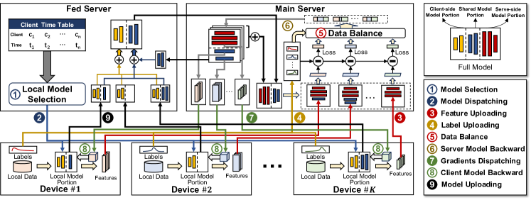
Inspired by the above intuitions, this paper presents a novel SFL approach, named Sliding Split Federated Learning (S²FL), which adopts a data balance-based training mechanism and an adaptive sliding model split strategy. In specific, in S²FL, to alleviate data heterogeneity, the main server recombines intermediate features according to their labels to ensure that each server-side model portion is trained by more IID features. To deal with stragglers, S²FL split the global model into three portions, i.e., the server-side model portion, the shared model portion, and the client-side model portion. At the beginning of each S²FL training round, the fed server splits the shared model portion according to the hardware resource of each AIoT device and dispatches the split shared model portion together with the client-side model portion to the corresponding device. In this way, AIoT devices with varying hardware capabilities can be dispatched different sizes of model portions, thus alleviating the training time differences caused by stragglers. The main contributions of this paper are as follows:

• We propose S²FL, a novel SFL framework, which adaptively splits models according to the device hardware resource to alleviate low training efficiency caused by straggers.

• We present a data balance-based training mechanism that enables the server-side model portion to be trained with a more balanced data distribution by grouping intermediate features based on their labels.

• We conduct experiments on various well-known datasets with various data heterogeneity scenarios to evaluate the effectiveness of our S²FL approach.

2. Related Work

Federated Learning (McMahan et al., 2017) (FL) is a distributed machine learning framework in 2016, which addresses data privacy problems by enabling each device to transmit models to the server instead of local data. However, in the AIoT scenario, different edge devices possess varying computational capabilities and data distributions. This will lead to problems such as stragglers and low inference accuracy due to data heterogeneity in FL. To address these problems, Xu et al.(Xu et al., 2021) proposed Helios, which assigns pruned models to weaker computational devices to synchronize fast and slow devices. Xie et al.(Xie et al., 2019) proposed FedAsync, which employs an asynchronous aggregation strategy to avoid inter-device waiting. Hsu et al.(Hsu et al., 2019) introduced a momentum-based solution to improve the inference accuracy under different data distributions. Although these works can effectively improve the efficiency or accuracy of FL, they require the client device to deploy a complete model. In the AIoT scenario with a large number of edge devices, devices with limited computational resources may not be able to independently train the complete model, and the transmission of complete models between a large number of devices and servers imposes a significant communication burden.

Split Learning (P.Vepakomma et al., 2018) (SL) divides the complete model into several parts, with each model part deployed on a separate client for computation. In SL, the clients with adjacent model parts transmit the intermediate feature which is the output of their own model’s last layer. When the model is large, SL effectively distributes the computing tasks to various clients, allowing clients that cannot independently load and train the complete model to participate in the model training. Furthermore, due to the smaller size of the feature compared to model parameters, SL has lower communication overhead compared to FL. Although SL has advantages when dealing with large models, the computation between clients is sequential, leading to a significant number of clients being idle during the training process. This results in a waste of computational resources and large training time overhead.

Split Federated Learning (Thapa et al., 2022) (SFL) combines the advantages of FL and SL. In SFL, the complete model is divided into two parts: the client-side model portion and the server-side model portion. Each client communicates directly with the main server and fed server. In each training round, clients interact with the main server in parallel to execute the SL process. Subsequently, clients send their updated client model portion to the fed server for aggregation. The fed server aggregates all clients’ models and synchronizes the aggregated model with all clients. However, a shortcoming of SFL is that it still experiences the problem of stragglers and low inference accuracy as in FL. Based on SFL, we proposed an adaptive sliding model split strategy and a data balance-based training mechanism that can effectively solve the problems in SFL.

3. Our Approach

Figure 1 presents the framework and workflow of S²FL, which consists of two servers (i.e., the fed server and the main server) and multiple AIoT edge devices. In S²FL, the full global model is divided into three portions, i.e., the client-side model portion, the server-side model portion, and the shared model portion, which are maintained by the fed server, the main server, and both the fed and the main servers, respectively. The fed server is used for the dispatching of client model portion and the aggregation of the client-side model and the shared model portions. As shown in Figure 1, the fed server includes a client time table, which maintains the average training time of each client. According to the client time table, the fed server splits a suitable size model portion from the shared model portion and dispatches it together with the client-side model portion as the client model portion to a specific AIoT device for model training. The main server is responsible for training the latter part of the model. It receives the features and labels uploaded by the client devices, continuing the forward and backward propagation of the model, and finally returning the gradient to each device.

As shown in Figure 1, the workflow of our approach includes the following nine steps:

• Step 1 (Model Selection): The fed server chooses a client model portion $W_{c}$ for each selected device based on the client time table, which includes the complete client-side model portion and partial layers of the shared model portion.

• Step 2 (Model Dispatching): The fed server dispatches the model portion $W_{c}$ to the selected devices for local training.

• Step 3 (Feature Uploading): Each device uses local data to perform forward propagation on the $W_{c}$ and upload the calculated features to the main server.

• Step 4 (Label Uploading): Each device uploads the labels of local data to the main server.

• Step 5 (Data Balance): When the main server has finished collecting features and labels, It uses the data balance-based training mechanism to group these features, and the main server will prepare the same number of copies of the server model portion $W_{s}$ as the number of groups, and the features in the same group will be input into the corresponding $W_{s}$ to calculate the loss.

• Step 6 (Server Model Backward): The main server aggregates all losses computed by each group, performs a backward propagation to update the corresponding $W_{s}$, and obtains the gradient of the features uploaded by each client device.

• Step 7 (Gradients Dispatching): The main server sends the gradient to the client device.

• Step 8 (Client Model Backward): After each device receives the gradient sent by the main server, it updates the client model portion $W_{c}$ with the gradient.

• Step 9 (Model Uploading): Each client sends the updated local model $W_{c}$ to the fed server for model aggregation.

Input: i) $r$, maximum number of rounds; ii) $C$, client set; iii) $\eta$, learning rate; iv) $[(Wc_{i},Ws_{i})|i=1..K]$, different size client model portion and server model portion;

Output: $W$, the full model

1 $\textbf{S}^{2}\textbf{FL}$ ($r$, $C$, $\eta$, $[(Wc_{i},Ws_{i})|i=1..K]$) begin

2 for $t$=1 to $r$ do

3       Random choose $x$ clients $(C_{1},C_{2},..C_{x})$ from $C$;

4       Using the adaptive sliding model split strategy to select a suitable $Wc_{i}$ for each client $C_{i}$, and send $Wc_{i}$ to $C_{i}$;

5       for $i$=1 to $x$ do

6             $D_{i}$ $\leftarrow$ Local data in $C_{i}$;

7             $(fx_{i},\mathscr{l}_{i})$ $\leftarrow$ $Wc_{i}$($D_{i}$);

8            

9       end for

10      $\mathcal{G}\_set$ $\leftarrow$ Use the data balance-based training mechanism to group all $fx$, and for each group,initialize a server model portion $W_{s}$ in $server\,model\,set$;

11       /* parallel for */

12       for $\mathcal{G}$ in $\mathcal{G}\_set$ do

13             for $i$ in $\mathcal{G}$ do

14                   $y_{i}$ = $W_{s}$($fx_{i}$);

15                   $loss_{i}=crossEntropy(y_{i},\mathscr{l}_{i})$;

16                  

17             end for

18            $loss=\cup_{i\in\mathcal{G}}loss_{i}$;

19             $W_{s}=W_{s}-\eta*\nabla(loss)$;

20             for $i$ in $\mathcal{G}$ do

21                   $dfx_{i}=\frac{\partial loss}{\partial fx_{i}}$;

22                  

23             end for

24            

25       end for

26      for $i$=1 to $x$ do

27             Send $dfx_{i}$ to $C_{i}$;

28             $Wc_{i}=Wc_{i}-\eta*\nabla(dfx_{i})$;

29             Save $Wc_{i}$ into $client\,model\,set$;

30            

31       end for

32      $W$ = Aggregation($client\,model\,set$,$server\,model\,set$);

33      

34 end for

35Return $W$;

end

Algorithm 1 Our $S^{2}FL$ approach

3.1. Implementation of Our Approach

Algorithm 1 presents the implementation of our approach. Line 3 selects $x$ clients from all clients to participate in this round of training. Line 4 uses the adaptive sliding model split strategy to choose a suitable client model portion $W_{c}$ for each client, making the training time of each client similar. Lines 5-7 represent each client performing forward propagation on their local data $D_{i}$ on $Wc_{i}$. The main server receives the features $fx_{i}$ and labels $\mathscr{l}_{i}$ sent by the clients. Line 8 uses the data balance-based training mechanism to group $fx$ based on the data distribution of clients and initializes a $W_{s}$ in the server model set for each group. Lines 9-17 represent the process of training for each group. For each $fx_{i}$ within the same group, line 12 inputs $fx_{i}$ into corresponding $W_{s}$ for forward propagation, obtaining the logits $y_{i}$. Line 13 calculates the $loss_{i}$ for each client using $y_{i}$ and $\mathscr{l}_{i}$. line14 combines all $loss_{i}$ to generate $loss$. Line 15 uses the $loss$ for backward propagation to update $W_{s}$. Lines 16-17 calculate the gradient $dfx_{i}$ for each $fx_{i}$, and lines 18-21 indicate that the main server sends the gradient $dfx_{i}$ to the corresponding client $C_{i}$. The client uses $dfx_{i}$ to update the client model portion $Wc_{i}$ and then uploads $Wc_{i}$ to the fed server. Fed server saves the $Wc_{i}$ into the client model set. Line 22 aggregates the models from both the client model set and the server model set to form the complete model $W$.

3.2. Adaptive Sliding Model Split Strategy

In the AIoT scenario, edge devices possess varying computational capabilities and network bandwidth. We measure them respectively using the floating-point operations per second (flops) and the transmission rates of each edge device. Assuming a complete model $W$ is divided into a client model portion $W_{c}$ and a server model portion $W_{s}$, where the size of $W_{c}$ is $|W_{c}|$, the output size of $W_{c}$’s final layer is $q$, and the floating-point computation counts for the forward and backward propagation of $W_{c}$ is $F_{c}$, while for $W_{s}$ it is denoted as $F_{s}$. The computation capability of the device is represented as $Comp_{c}$, with a transmission rate of $R$ and a local data quantity of $p$. The computation capability for the server is denoted as $Comp_{s}$. In our workflow, a complete training iteration starts with the fed server sending $W_{c}$ to the device and ends when the fed server receives the uploaded $W_{c}$ from the device. Under our assumptions, the time $T$ required for a single device to complete one round of training becomes:

(1) $$T=\frac{2|W_{c}|+2pq}{R}+\frac{F_{c}}{Comp_{c}}+\frac{F_{s}}{Comp_{s}}$$

When each device trains the same $W_{c}$ and the same quantity $p$ of local data, high-performance devices with faster computational speed $Comp_{c}$ and higher transmission rate $R$ will be able to complete training more quickly, which causes high-performance devices to need to wait for other devices. To address this problem, the fed server will dynamically select the model portion that is appropriate for each device’s computational resources so that the time $T$ spent on a training round is similar between devices. Specifically, in order to match devices with different computational resources, we set up $K$ possible split layers, in the first $K$ rounds of our approach, the fed server traverses all the split layers and uses one of them to divide $W$ into $W_{c}$ and $W_{s}$ within a same round, then it sends $W_{c}$ to all the devices and turns on a timer. When the fed server receives a $W_{c}$ uploaded by a device, it then records the time spent by that device this round in its own client time table. The client time table is a table for evaluating the computational resources of each device, which records for each device the time it takes to complete a training round when training different sizes of $W_{c}$. After the warm-up phase of round $K$, the fed server will select a subset of devices (assume $x$ devices) to participate in training in each round, and it will collect the time spent by these devices of training on each different $W_{c}$ from the client time table, and take the median of these times (total has $x*K$ times). Then, for each device, the fed server selects $W_{c}$ with the training time closest to the median as the client model portion used for this round of training. When the fed server receives the model uploaded by the device in this round, it dynamically updates the client time table based on the size of the client model portion and the training time.

Figure 2. Data balance-based training mechanism

3.3. Data Balance-based Training Mechanism

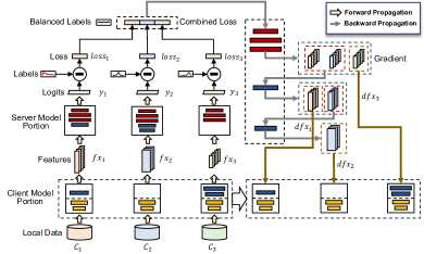
To address the problem of low inference accuracy caused by data heterogeneity, as shown in Figure 2, we present a data balance-based training mechanism. Assume that the dataset $D=[D^{(1)},D^{(2)},D^{(3)},...,D^{(n)}]$ consists of data with $n$ categories, where $D^{(i)}$ represents the data set with the label $i$. When the main server receives the intermediate features $fx$ and their labels $\mathscr{l}$ from the client device, it gets the data distribution of the client through $\mathscr{l}$. Next, the main server groups the $fx$ uploaded by devices. Specifically, for $x$ clients participating in each round of training, the main server groups the $fx$ uploaded by clients whose combined data distribution is closest to the uniform distribution. In other words, we sum and normalize the data distribution of devices and then calculate the L2 distance from the uniform distribution as follows:

(2) $$Dist=\sqrt{\sum^{n}_{i=1}{(\frac{\sum_{c\in\mathcal{G}}|D^{(i)}_{c}|}{\sum_{p\in\mathcal{G}}|D_{p}|}-\frac{1}{n})^{2}}},$$

where $\mathcal{G}$ denotes a group of devices, $|D^{(i)}_{c}|$ denotes the quantity of data with the label $i$ in client $c$, $|D_{p}|$ indicates total amount of data for the client $p$. Note that the goal of our grouping is to minimize the distance. After the grouping process, $fx$ in the same group inputs into the same server model portion $W_{s}$ for training. As shown in Figure 2, the intermediate features $fx_{i}$ within the same group are first input into $W_{s}$ for forward propagation to obtain logits $y_{i}$. Then, the main server uses $y_{i}$ with $\mathscr{l}_{i}$ to calculate $loss_{i}$ using a specific loss function (e.g., cross entropy). Next, the main server combines calculated losses in a group to generate the combined loss as follows:

(3) $$loss=\cup_{i\in group}loss_{i}.$$

The main server performs backward propagation to update the server model portion $W_{s}$, calculates the gradient $dfx_{i}$ of each $fx_{i}$ based on the combined $loss$, and sends the $dfx_{i}$ to the corresponding device for local $W_{c}$ updating. The above process can be presented as follows:

(4) $$W_{s}=W_{s}-\eta*\nabla(loss),dfx_{i}=\frac{\partial loss}{\partial fx_{i}},Wc_{i}=Wc_{i}-\eta*\nabla(dfx_{i})$$

3.4. Model Aggregation

In S²FL, the model is divided into three parts: client-side model portion, shared model portion, and server-side model portion. The layer of the shared model portion can be split into the server model $W_{s}$ or client model $W_{c}$. As a result, S²FL cannot use the simple weighted average to aggregate models like FedAvg. Algorithm 2 presents our model aggregation method. Line 2 obtains the data size of $x$ devices participating in training. Lines 3-10 traverse each $layer$ of the full model $W$. For each client model portion $Wc_{i}$ in the client model set, if the $Wc_{i}$ has the $layer$, then the $Wc_{i}[layer]$ is used to participate in the model aggregation. If $W_{c}$ doesn’t have the $layer$, we use the $layer$ in $W_{s}$ that corresponds to $Wc_{i}$ in the server model set to participate in model aggregation. In both cases, the weight is set to the data size of device $|D_{i}|$. Lines 11-12 average the aggregated model $W$.

Input: i) $C$, the client model set; ii) $S$, the server model set;

Output: $W$, the full model

1 Aggregation ($C$, $S$) begin

2 $(|D_{1}|,|D_{2}|,..,|D_{x}|)\leftarrow$ Data size of each device ;

3 for $layer$ in $W$ do

4       for $Wc_{i}$ in $C$ do

5             if $Wc_{i}$ has $layer$ then

6                   $W[layer]=W[layer]+|D_{i}|\times Wc_{i}[layer]$;

7                  

8             end if

9            else

10                   $W_{s}$ $\leftarrow$ the corresponding model to $Wc_{i}$ in $S$;

11                   $W[layer]=W[layer]+|D_{i}|\times W_{s}[layer]$;

12                  

13             end if

14            $weight[layer]=weight[layer]+|D_{i}|$;

15            

16       end for

17      

18 end for

19for $layer$ in $W$ do

20       $W[layer]=W[layer]/weight[layer]$

21 end for

22Return $W$;

end

Algorithm 2 Model aggregation

4. Experimental Results

To evaluate the effectiveness of $S^{2}FL$, we implemented our approach using the PyTorch framework. We compared $S^{2}FL$ with both classical FedAvg and the SFL. We select three different split layers on each used model $W$, dividing $W$ into three different client and server model portion tuples:[$(Wc_{1},Ws_{1})$, $(Wc_{2},Ws_{2})$, $(Wc_{3},Ws_{3})$] where $size(Wc_{1})<size(Wc_{2})<size(Wc_{3})$. Devices train the complete model $W$ in FedAvg and train the largest client model portion $Wc_{3}$ in SFL. Our approach uses the adaptive sliding model split strategy to choose a suitable client model portion for each device. To enable fair comparison, we set the batch size to 128 and used an SGD optimizer with a learning rate of 0.01 for both all the baselines and $S^{2}FL$. All the experimental results were obtained from an Ubuntu workstation with an Intel i9 CPU, 64GB memory, and an NVIDIA RTX 3090 GPU.

4.1. Experimental Settings

1) Settings of Devices: We set the flops and transfer rate of each device to measure the computing power and network bandwidth of these devices. In the experiment, we assume that there are three different flops and three different transfer rates. Table 1 shows the settings of flops and transfer rates. Each device has a specific quality of flopS and transfer rate in this table. Because flops and transfer rate are not correlated, there are a total of 9 different kinds of devices in our experiment. We assume that the server has ultra-high computing resources, its flops is set to $5\times 10^{10}$, and the transfer rate is set to $1\times 10^{7}$.

Table 1. Devices settings

Quality	Flops Settings	Transfer Rate Settings
Low	$5\times 10^{9}$	$1\times 10^{6}$
Mid	$1\times 10^{10}$	$2\times 10^{6}$
High	$2\times 10^{10}$	$5\times 10^{6}$

2) Settings of Datasets and Models: We compared the performance of our approach and two baselines on three well-known datasets, i.e., CIFAR-10, CIFAR-100, and FEMNIST (Caldas et al., 2018). To investigate the performance of our approach on the no-IID scenarios, we use the Dirichlet distribution to control the data heterogeneity between devices on datasets CIFAR-10 and CIFAR-100 and set a parameter $a$ to indicate the degree of heterogeneity, and for datasets FEMNIST, we use its natural no-IID distribution. For experiments on datasets CIFAR-10 and CIFAR-100, we assume that there are 100 AIoT devices and 10 devices are randomly selected for local training in each training round. However, for dataset FEMNIST, there are a total of 180 devices and each training round involves 18 devices. In addition, to show the pervasiveness of our approach, we experimented on three different DNN models(i.e., ResNet-8, VGG-16, and mobileNet).

(a) $a=0.1$

(b) $a=0.5$

(c) $a=1.0$

(d) $IID$

Figure 3. Training process of $S^{2}FL$ and two baselines on CIFAR-10

Table 2. Comparison of test accuracy

Dataset	Model	Hetero. Settings	Test Accuracy(%)
			FedAvg	SFL	$S^{2}FL$(ours)
CIFAR-10	ResNet8	$a=0.1$	$48.65\pm 1.16$	$49.13\pm 1.70$	$\textbf{51.87}\pm\textbf{1.70}$
		$a=0.5$	$56.96\pm 0.31$	$58.15\pm 0.32$	$\textbf{60.43}\pm\textbf{0.38}$
		$a=1.0$	$58.72\pm 0.27$	$60.48\pm 0.20$	$\textbf{62.78}\pm\textbf{0.19}$
		$IID$	$59.52\pm 0.15$	$62.02\pm 0.07$	$\textbf{64.08}\pm\textbf{0.09}$
	VGG16	$a=0.1$	$51.61\pm 1.73$	$52.50\pm 3.21$	$\textbf{58.94}\pm\textbf{1.58}$
		$a=0.5$	$65.53\pm 0.27$	$66.04\pm 0.35$	$\textbf{72.45}\pm\textbf{0.21}$
		$a=1.0$	$68.67\pm 0.29$	$68.96\pm 0.36$	$\textbf{74.65}\pm\textbf{0.20}$
		$IID$	$68.57\pm 0.11$	$70.15\pm 0.06$	$\textbf{75.12}\pm\textbf{0.09}$
	mobileNet	$a=0.1$	$35.68\pm 0.62$	$36.68\pm 0.42$	$\textbf{38.19}\pm\textbf{0.83}$
		$a=0.5$	$47.85\pm 0.55$	$49.01\pm 0.41$	$\textbf{52.80}\pm\textbf{0.26}$
		$a=1.0$	$52.29\pm 0.57$	$52.08\pm 0.35$	$\textbf{58.33}\pm\textbf{0.34}$
		$IID$	$55.56\pm 0.15$	$55.21\pm 0.08$	$\textbf{61.61}\pm\textbf{0.13}$
CIFAR-100	ResNet8	$a=0.1$	$29.72\pm 0.30$	$27.15\pm 0.15$	$\textbf{34.90}\pm\textbf{0.23}$
		$a=0.5$	$31.72\pm 0.09$	$28.52\pm 0.15$	$\textbf{38.31}\pm\textbf{0.10}$
		$a=1.0$	$31.40\pm 0.09$	$28.72\pm 0.14$	$\textbf{38.22}\pm\textbf{0.21}$
		$IID$	$31.21\pm 0.06$	$28.19\pm 0.09$	$\textbf{38.61}\pm\textbf{0.08}$
	VGG16	$a=0.1$	$33.24\pm 0.76$	$30.55\pm 0.42$	$\textbf{44.04}\pm\textbf{0.44}$
		$a=0.5$	$31.22\pm 0.19$	$27.85\pm 0.21$	$\textbf{44.34}\pm\textbf{0.18}$
		$a=1.0$	$31.90\pm 0.17$	$28.31\pm 0.28$	$\textbf{44.49}\pm\textbf{0.13}$
		$IID$	$32.21\pm 0.05$	$29.48\pm 0.09$	$\textbf{44.60}\pm\textbf{0.15}$
	mobileNet	$a=0.1$	$16.69\pm 0.24$	$15.40\pm 0.21$	$\textbf{21.15}\pm\textbf{0.13}$
		$a=0.5$	$18.36\pm 0.10$	$15.51\pm 0.05$	$\textbf{23.31}\pm\textbf{0.09}$
		$a=1.0$	$18.24\pm 0.10$	$16.24\pm 0.09$	$\textbf{23.30}\pm\textbf{0.09}$
		$IID$	$19.10\pm 0.07$	$16.74\pm 0.10$	$\textbf{23.17}\pm\textbf{0.09}$
FEMNIST	ResNet8	$-$	$80.22\pm 0.07$	$79.46\pm 0.11$	$\textbf{82.01}\pm\textbf{0.13}$
	VGG16	$-$	$82.99\pm 0.16$	$82.03\pm 0.11$	$\textbf{84.28}\pm\textbf{0.22}$
	mobileNet	$-$	$72.99\pm 0.15$	$73.37\pm 0.14$	$\textbf{79.75}\pm\textbf{0.14}$

4.2. Performance Comparison

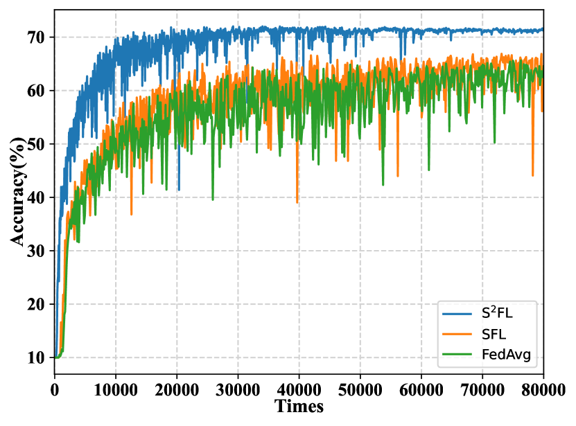
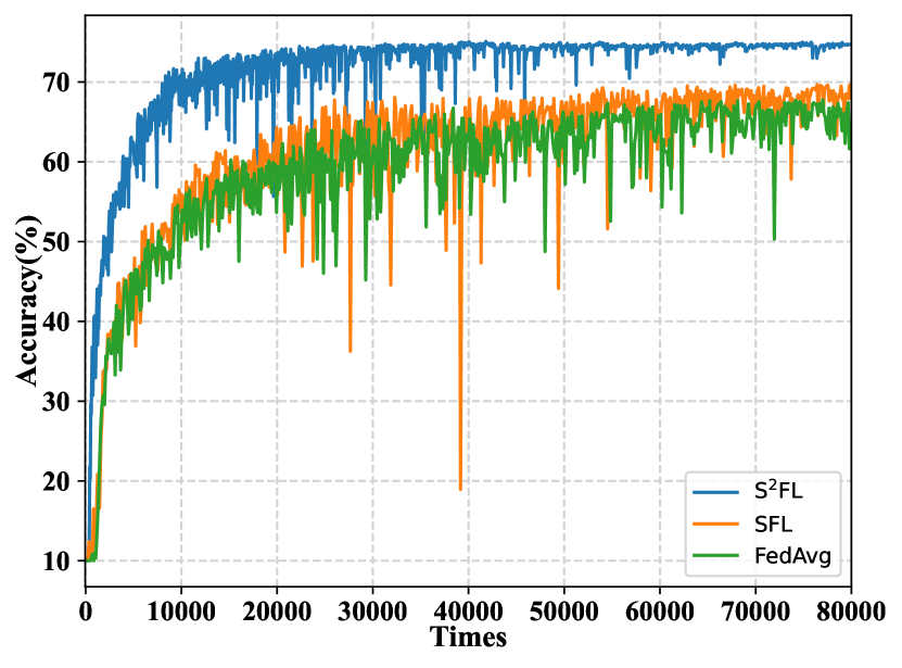
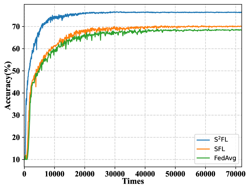
1) Comparison of Accuracy: Table 2 compares the test accuracy of our method and all baselines at IID and non-IID settings. From the table, we find that our method achieves the best accuracy in all cases. Noting that SFL is actually equivalent to FedAvg, so they have similar accuracy. Compared to SFL, the test accuracy of our approach is up to 16.5% higher on the CIFAR-100 dataset with the VGG16 model when $a=0.5$. Figure 2 shows the training process of $S^{2}FL$ and two baselines on CIFAR-10 based on the VGG16 model. We can find that our approach achieves the highest accuracy and has a more stable learning curve in both no-IID and IID scenarios.

2) Comparison of Training Convergence Speed and Communication Overhead: We consider the time and communication overhead required to achieve a certain accuracy during training. Table 3 compares our method with two baselines, all of them training VGG16 on the CIFAR-10 dataset. As can be seen from the table, when training the large model (such as VGG16), SFL reduces the training time of the device by letting the device train a model portion, and because the output feature size of the model portion is smaller than the parameters of the entire model, SFL has a faster convergence speed and smaller communication overhead than FL. Our approach mitigates the problem of straggles in SFL and reduces the training time and communication overhead, $S^{2}FL$ outperforms SFL by 3.54X and 2.57X in terms of training time and communication overhead when $a=0.5$.

Table 3. Comparison of training time and communication overhead

Hetero. Settings	Acc.%	FedAvg		SFL		$S^{2}FL$
		Time	Comm.	Time	Comm.	Time	Comm.
$a=0.1$	40	21299s	29936M	13763s	12224M	8471s	11372M
	50	41436s	61083M	35294s	32999M	19471s	27599M
$a=0.5$	50	8162s	19655M	7612s	11958M	2338s	5142M
	60	21320s	51104M	16022s	25300M	4524s	9826M
$a=1.0$	55	10498s	24191M	9329s	14378M	2908s	6381M
	60	15162s	34472M	10058s	15423M	3921s	8512M
$IID$	60	10614s	26913M	8963s	15423M	2952s	6823M
	65	16020s	40520M	13422s	23047M	3967s	9151M

4.3. Impacts of Different Configurations

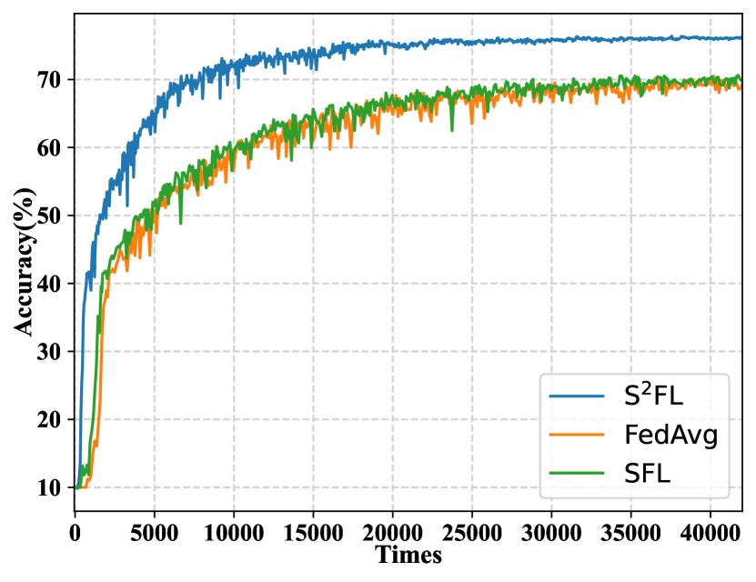
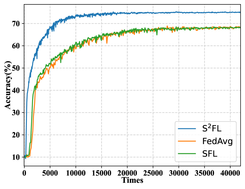
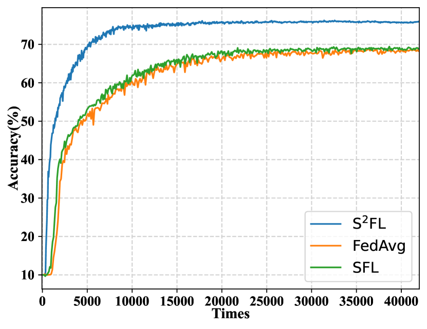
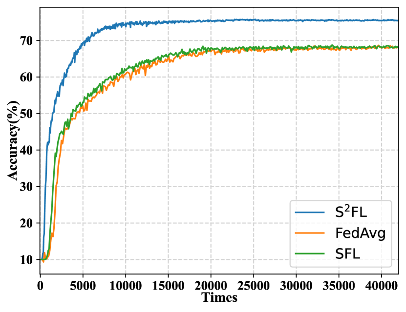
1)Impacts of the number of participating devices. We explored the impact of the number of devices $x$ participating in each round of training. We conducted experiments on four cases where x is equal to 5, 10, 15, and 20. Figure 4 shows the training process conducted on CIFAR-10 with IID distribution using VGG16. We observed that our approach achieved the highest accuracy across all cases, and as the number of devices increased, our approach had a higher accuracy improvement than other baselines.

(a) $x=5$

(b) $x=10$

(c) $x=15$

(d) $x=20$

Figure 4. Training processes with different numbers of devices

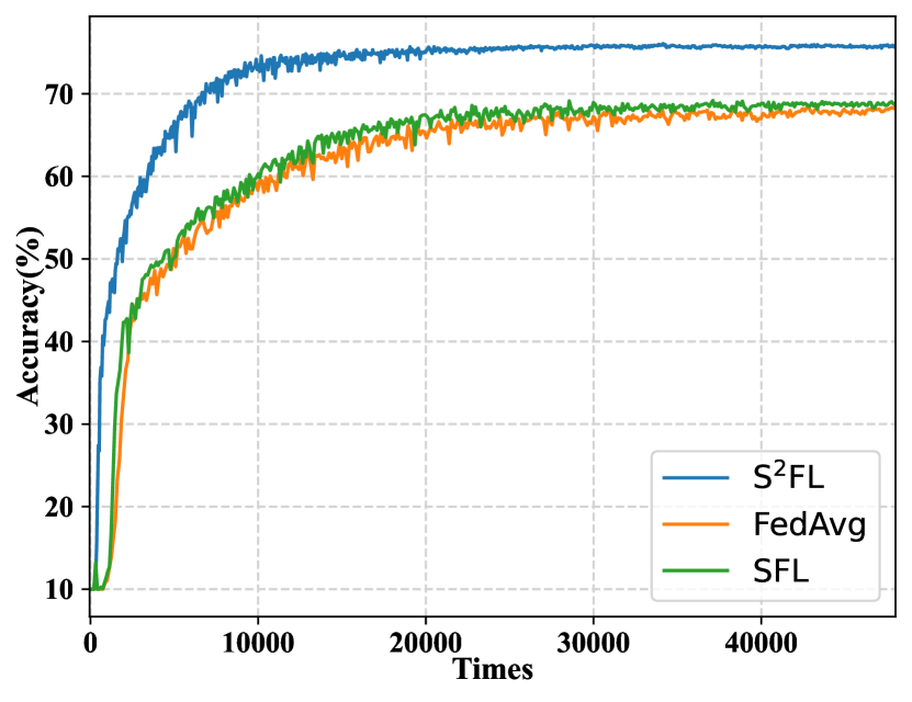
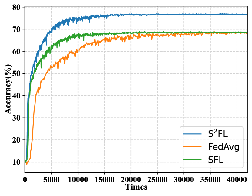
2) Impacts of Device Compositions. We consider the effectiveness of our approach in different device composition scenarios. We used two different configurations in our experiment: conf 1), High: Mid: Low = 5: 3: 2 in both flops settings and transfer rate settings. conf 2), High: Mid: Low = 2: 3: 5 in both flops settings and transfer rate settings. Figure 5 shows the training process conducted on CIFAR-10 with IID distribution using VGG16. We observed that when the proportion of low flopS and low transfer rate devices increased, $S^{2}FL$ and $SFL$ that allowed the device to train only part of the model achieved faster convergence. The $S^{2}FL$ achieves the highest accuracy in both configurations.

(a) $conf1$

(b) $conf2$

Figure 5. Training processes with different device compositions

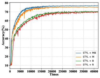
3) Ablation Study. To demonstrate the effectiveness of our adaptive sliding model split strategy and the data balance-based training mechanism, we conducted experiments on four different configurations of $S^{2}FL$: 1) $S^{2}FL+R$, which does not use the adaptive sliding model split strategy and the data balance-based training mechanism in $S^{2}FL$, note that this configuration is equivalent to SFL. 2) $S^{2}FL+B$ that uses the data balance-based training mechanism. 3) $S^{2}FL+M$ that uses the adaptive sliding model split strategy. 3) $S^{2}FL+MB$ that enables both the adaptive sliding model split strategy and the data balance-based training mechanism. Figure 6 shows the ablation study results on the CIFAR-10 dataset with VGG16 following IID distribution. We can observe that $S^{2}FL+MB$ achieves the highest accuracy rate across all configurations. $S^{2}FL+M$ has a faster convergence speed than $S^{2}FL+R$, which indicates that our adaptive sliding model split strategy can effectively synchronize the training time between devices and speed up the training speed. $S^{2}FL+B$ has a higher test accuracy than $S^{2}FL+R$, which indicates that our data balance-based training mechanism can alleviate the problem of inference accuracy degradation caused by data heterogeneity.

Figure 6. Ablation study in $S^{2}FL$

5. Conclusion

Although FL is increasingly used in AIoT scenarios, it still has the problem that resource-constrained devices cannot support large-size models. Some existing solutions such as SFL do not consider the problem of stragglers and data heterogeneity. To address this problem, we propose an effective and accurate approach called S²FL based on SFL. It uses our proposed adaptive sliding model split strategy to select the model portion for the device that matches its computing resources so that the training time is similar between the devices. At the same time, S²FL uses the data balance-based training mechanism to group devices, letting the model be trained on a more uniform data distribution. Comprehensive experiments show that our approach can achieve faster convergence speed and higher inference accuracy compared with state-of-the-art methods.

References

- (1)
- Caldas et al. (2018) S. Caldas et al. 2018. LEAF: A Benchmark for Federated Settings. arXiv.
- Chang et al. (2021) Z. Chang et al. 2021. A survey of recent advances in edge-computing-powered artificial intelligence of things. IEEE IoTJ 8, 18 (2021), 13849–13875.
- Ghosh et al. (2020) A. Ghosh et al. 2020. An efficient framework for clustered federated learning. Proc. of NeurIPS 33, 19586–19597.
- Hsu et al. (2019) T. H. Hsu et al. 2019. Measuring the Effects of Non-Identical Data Distribution for Federated Visual Classification. arXiv preprint arXiv:1909.06335.
- Hu et al. (2023) M. Hu et al. 2023. AIoTML: A Unified Modeling Language for AIoT-Based Cyber-Physical Systems. IEEE TCAD 42, 11 (2023), 3545–3558.
- Karimireddy et al. (2020) S. P. Karimireddy et al. 2020. Scaffold: Stochastic controlled averaging for federated learning. In Proc. of ICML. 5132–5143.
- Li et al. (2020) B. Li et al. 2020. DeepFed: Federated deep learning for intrusion detection in industrial cyber-physical systems. IEEE TII 17, 8 (2020), 5615–5624.
- Li et al. (2019) L. Li et al. 2019. SmartPC: Hierarchical pace control in real-time federated learning system. In Proc. of RTSS. 406–418.
- McMahan et al. (2017) B. McMahan et al. 2017. Communication-efficient learning of deep networks from decentralized data. In Proc. of AISTATS. 1273–1282.
- P.Vepakomma et al. (2018) P.Vepakomma et al. 2018. Split learning for health: Distributed deep learning without sharing raw patient data. arXiv preprint arXiv:1812.00564.
- Thapa et al. (2022) C. Thapa et al. 2022. Splitfed: When federated learning meets split learning. In In Proc. of AAAI, Vol. 36. 8485–8493.
- Xie et al. (2019) C. Xie et al. 2019. Asynchronous federated optimization. arXiv preprint arXiv:1903.03934.
- Xu et al. (2021) Z. Xu et al. 2021. Helios: Heterogeneity-Aware Federated Learning with Dynamically Balanced Collaboration. In Proc. of DAC. 997–1002.
- Zhang et al. (2020) X. Zhang et al. 2020. Efficient federated learning for cloud-based AIoT applications. IEEE TCAD 40, 11 (2020), 2211–2223.
- Zhu et al. (2021) Z. Zhu et al. 2021. Data-free knowledge distillation for heterogeneous federated learning. In Proc. of ICML. PMLR, 12878–12889.