Single Image Compressed Sensing MRI via a Self-Supervised Deep Denoising Approach

Abstract

Popular methods in compressed sensing (CS) are dependent on deep learning (DL), where large amounts of data are used to train non-linear reconstruction models. However, ensuring generalisability over and access to multiple datasets is challenging to realise for real-world applications. To address these concerns, this paper proposes a single image, self-supervised (SS) CS-MRI framework that enables a joint deep and sparse regularisation of CS artefacts. The approach effectively dampens structured CS artefacts, which can be difficult to remove assuming sparse reconstruction, or relying solely on the inductive biases of CNN to produce noise-free images. Image quality is thereby improved compared to either approach alone. Metrics are evaluated using Cartesian 1D masks on a brain and knee dataset, with PSNR improving by 2-4dB on average.

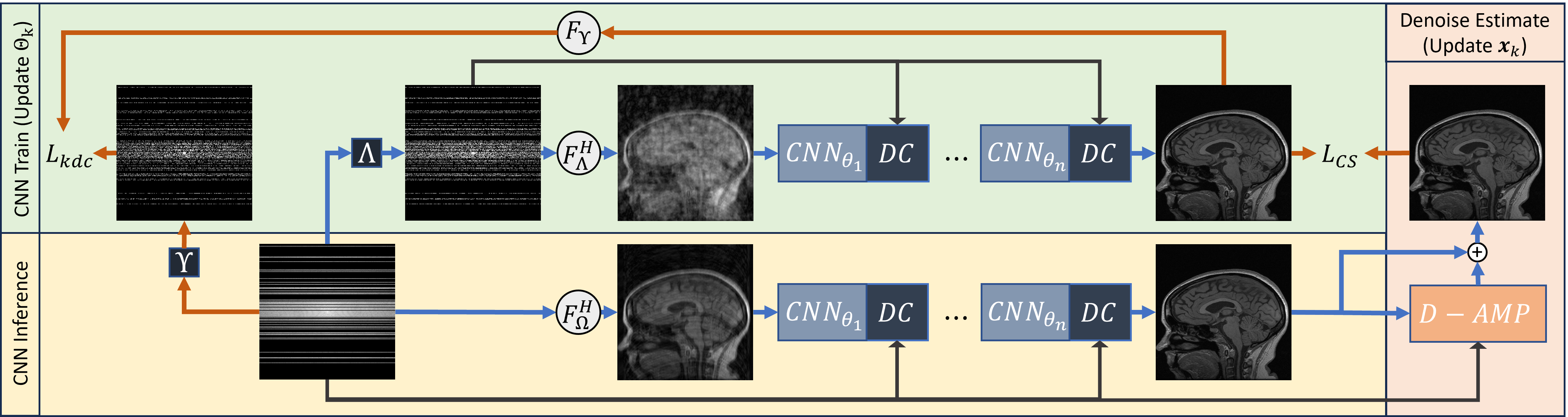
Fig. 1: Proposed single image, self-supervised training procedure. Each epoch, sampled $k$-space $\mathbf{y}_{\_}\Omega$ is divided into subsets $\mathbf{y}_{\_}\Lambda,\mathbf{y}_{\_}\Upsilon$. Image estimates $\hat{\mathbf{x}}_{\_}\Lambda=f(F_{\_}\Lambda^{H}\mathbf{y}_{\_}\Lambda|\Theta_{\_}k)$ and $\hat{\mathbf{x}}_{\_}\Omega=f(F_{\_}\Omega^{H}\mathbf{y}_{\_}\Omega|\Theta_{\_}k)$ are then generated. CNN and DC blocks are described in Eq. 4, where $\Theta_{\_}k=\{\theta_{\_}t\}_{\_}{t=1}^{n}$ at epoch $k$. The MSE between $\hat{\mathbf{x}}_{\_}\Lambda$ and the denoiser estimate $\mathbf{x}_{\_}k$ ($L_{\_}{CS}:=\frac{\mu}{2}\|\mathbf{x}_{\_}k-\hat{\mathbf{x}}_{\_}\Lambda-\mathbf{q}_{\_}k\|_{\_}2^{2}$), as well as withheld $k$-space $\mathbf{y}_{\_}\Upsilon$ ($L_{\_}{kdc}:=\|\mathbf{y}_{\_}\Upsilon-F_{\_}\Upsilon\mathbf{\hat{x}}_{\_}\Lambda\|_{\_}2^{2}$), are used to update $\mathrm{\Theta}$ (Eq. 9). $\mathbf{q}_{\_}k$ is the Lagrange multipliers vector. Rather than relying on the inherent bias of CNN to produce noise-free images via $L_{\_}{kdc}$, inclusion of $L_{\_}{CS}$ ensures the solution is noise-free with respect to the chosen CS-MRI algorithm.

1 Introduction

MRI is a medical imaging technique that captures detailed cross-sectional images of the body without ionizing radiation. However, the process of acquiring data is slow compared to other modalities due to physical and biological factors. A popular method of acceleration is via $k$-space (discrete Fourier space) under-sampling. Importantly, sampling schemes are constrained to continuous trajectories through $k$-space, which can lead to structured image artefacts. Many hand-crafted recovery techniques have been proposed that produce high-quality images, relevant for this work are algorithms based on compressed sensing (CS) [1, 2, 3]. Recently, the advent of deep learning (DL) has delivered significant contributions for medical image recovery, enabling a data-driven approach to solve difficult inverse problems [4, 5, 6].

Although image quality has benefited from DL, there are still questions regarding generalisability over multiple datasets, considering fully-sampled training data is not always guaranteed. SS procedures mitigate this deficiency by training DL CS- Magnetic resonance imaging (MRI) models from large datasets of under-sampled measurements [7, 8, 9, 10]. However, out of domain reconstruction remains a concern [11]. Foregoing training examples altogether, Deep Image Prior (DIP) exploits the inductive biases of convolutional neural network (CNN) architectures to solve single image inverse problems, leveraging the relationship between the reconstructed image and the image degradation model [12]. ConvDecoder [13] and Zero-Shot Self-Supervised Learning (ZS-SSL) [11] are examples of DIP-style solutions to CS-MRI. Importantly, ZS-SSL improves upon DIP via a loss function that is reminiscent of Self2Self With Dropout [14] and variational recovery; convergence guarantees remain a topic of interest [11]. The robustness of DIP was later improved with DeepRED [15], which combines with regularisation by denoising (RED) [16] to help guide the reconstruction process. While DeepRED is capable of producing high quality images, performance is dependent on the suitability of the chosen denoiser to the image degradation model. Unfortunately, structured CS artefacts are often difficult to remove assuming a Gaussian noise distribution [2].

Recognising that sparse regularisation is effective for CS [3], this work proposes a deep and sparse self-supervised (SS)-CS-MRI framework that improves the regularisation of single image SS CNN without requiring training data. Our algorithm can be described as a DeepRED-style approach, where a CNN prior is trained on the degraded measurements (similar to DIP), while a hand-crafted CS algorithm guides the reconstruction. Inclusion of the CS algorithm ensures robustness in the final solution, as hand-crafted techniques are characterised by recovery guarantees and predictable behaviour [17]. This ensures the reconstruction is not solely dependent on the inherent bias of CNN to produce noise-free images. Rather, well-known image characteristics that are embedded into CS algorithms are also leveraged. We emphasize that the proposed technique is compatible with existing denoising CNN and CS-MRI algorithms by deploying the popular Deep Cascade of Convolutional Neural Networks (DcCNN) [4] as the CNN to be trained on a single image, and denoising-based approximate message passing (D-AMP) [2] as the CS technique.

2 Methods

CS-MRI is often an iterative solution to,

$$\min_{\_}\mathbf{x}\|F_{\_}\Omega\mathbf{x}-\mathbf{y}_{\_}\Omega\|_{\_}2^{2}+\lambda\mathcal{R}(\mathbf{x}),$$ (1)

where $F_{\_}\Omega$ represents the masked two dimensional (2D) discrete Fourier transform (DFT) at locations $\Omega$, $\mathbf{y}_{\_}\Omega$ is under-sampled $k$-space and $\mathcal{R}(\cdot)$ is some regularisation function [1]. This work will investigate D-AMP and DcCNN for use in our SS-CS-MRI.

D-AMP is a CS algorithm that replaces $\mathcal{R}(\cdot)$ in Eq. 1 with the prior inherent to Gaussian denoisers [2]. Construction of D-AMP begins by considering the iterative shrinkage-thresholding algorithm (ISTA) solution to Eq. 1,

$$\begin{split}\mathbf{r}_{\_}t&=\hat{\mathbf{x}}_{\_}{t}+F_{\_}\Omega^{H}(\mathbf{y}_{\_}\Omega-F_{\_}\Omega\hat{\mathbf{x}}_{\_}{t}),\\ \hat{\mathbf{x}}_{\_}{t+1}&=\operatorname*{arg\,min}_{\_}\mathbf{x}\frac{1}{2}\|\mathbf{x}-\mathbf{r}_{\_}{t}\|_{\_}2^{2}+\lambda_{\_}t\mathcal{R}(\mathbf{x}).\end{split}$$ (2)

It is easy to see that the $\operatorname*{arg\,min}_{\_}\mathbf{x}\frac{1}{2}\|\mathbf{x}-\mathbf{r}_{\_}t\|_{\_}2^{2}+\lambda_{\_}t\mathcal{R}(\mathbf{x})$ term resembles the maximum a posteriori (MAP) estimation of $\mathbf{r}$. If we assume the residual $\mathbf{x}-\mathbf{r}_{\_}t$ has Gaussian distribution, then one could simply deploy existing Gaussian image denoising algorithms such as block-matching and 3D filtering (BM3D) to regularise the solution,

$$\hat{\mathbf{x}}_{\_}{t+1}=D_{\_}\sigma(\mathbf{r}_{\_}t),$$ (3)

with $D_{\_}\sigma(\cdot)$ being the chosen Gaussian denoiser and $\sigma$ a hyper-parameter for standard deviation of noise. Unfortunately, successive calls to $D_{\_}\sigma(\cdot)$ biases intermediate solutions to remove “‘observable” Gaussian noise in the residual, limiting the effectiveness of Gaussian denoising and slowing convergence [2]. D-AMP not only ensures the residual retains a Gaussian distribution between iterations, it is also capable of estimating the standard deviation of noise $\hat{\sigma}_{\_}t$ by means of the Onsager correction term [2]. In the context of MRI and Eq. 2, then $F_{\_}\Omega(\mathbf{r}_{\_}{t-1}-\hat{\mathbf{x}}_{\_}{t-1})\text{div}D_{\_}{\hat{\sigma}_{\_}{t-1}}(\mathbf{r}_{\_}{t-1})/m$ is the Onsager correction term and $m$ is the total number of sampled points in $\Omega$. We have implemented this algorithm using Python’s NumPy and the BM3D denoising algorithm.

DcCNN follows a DL-CS paradigm that unrolls an iterative reconstruction scheme into a series of CNN denoising and data consistency (DC) steps. We implement the network as follows,

$$\begin{split}\mathbf{x}_{\_}{t}&=f(\hat{\mathbf{x}}_{\_}{t}|\theta_{\_}t)\\ \hat{\mathbf{x}}_{\_}{t+1}&=F^{H}(F_{\_}{\bcancel{\Omega}}\mathbf{x}_{\_}t\cup\mathbf{y}_{\_}\Omega)\end{split}$$ (4)

where $f(\cdot|\theta_{\_}t)$ is the denoising CNN at iteration $t$ with weights $\theta_{\_}t$, $\bcancel{\Omega}$ indicates the set of points not in $\Omega$. DC therefore replaces $k$-space coefficients of $\mathbf{x}_{\_}{t}$ with known measurements $\mathbf{y}_{\_}\Omega$ in each iteration, whilst keeping the CNN generated samples in $\bcancel{\Omega}$. We express a call to this network as,

$$\hat{\mathbf{x}}_{\_}\Omega=f(F_{\_}\Omega^{H}\mathbf{y}_{\_}\Omega|\Theta),$$ (5)

where $\Theta=\{\theta_{\_}t\}_{\_}{t=1}^{n}$ is the set of network weights in all iterations and $F_{\_}\Omega^{H}\mathbf{y}_{\_}\Omega$ is the zero-filled (ZF) estimate. The authors originally propose to train this network by computing the mean squared error (MSE) between reconstructed and ground truth images within a large dataset. We instead propose a deep and sparse single image SS-CS-MRI loss (see Fig. 1).

2.1 Self-Supervised DL-MRI

Similar to ZS-SSL [11], our SS uses the corrupted image and knowledge of the degradation process (under-sampled $k$-space) to train an image recovery model. Each epoch, $\Omega$ is divided into randomly generated $\Lambda$ and $\Upsilon$, such that $\Omega=\Lambda\cup\Upsilon$; ZS-SSL uses a fixed $K$ pairs of $\Lambda$ and $\Upsilon$ with an additional ‘validation’ set $\Gamma$ to detect over-fitting. The CNN denoiser $f(\cdot|\Theta)$ is therefore trained to recover $\Upsilon$ from $\Lambda$, ensuring network outputs from each randomly generated subset are projected onto the same image. Due to the bias of CNN to produce noise-free images [12], it is hoped that the reconstruction converges to the original fully-sampled image rather than the ZF solution. The “deep” component of our SS loss is therefore defined as,

$$L_{\_}{kdc}:=\|\mathbf{y}_{\_}\Upsilon-F_{\_}\Upsilon\mathbf{\hat{x}}_{\_}\Lambda\|_{\_}2^{2}$$ (6)

where,

$$\mathbf{\hat{x}}_{\_}\Lambda=f(F_{\_}\Lambda^{H}\mathbf{y}_{\_}\Lambda|\Theta).$$ (7)

While Eq. 6 is still prone to over-fitting to the ZF data, ZS-SSL [11] demonstrated that this single-image SS paradigm results in higher-quality images than the original DIP [12] (and ConvDecoder [13]). We also find that randomly dividing $\Omega$ each epoch rather than using a fixed set of $K$ training pairs improved convergence characteristics and removed the need for an additional validation set.

2.2 Self-Supervised DL-CS-MRI

To leverage the non-linearity of CNN for single image applications and ensure the model does not converge to the ZF solution, we improve SS via the following DeepRED-style optimisation function,

$$\min_{\_}{\mathbf{x},\Theta}\frac{1}{2}L_{\_}{kdc}+\frac{\lambda}{2}\mathbf{x}^{H}(\mathbf{x}-g(\mathbf{x},\mathbf{y}_{\_}\Omega))\;\;\;s.t.\;\mathbf{x}=f(\cdot|\Theta)$$ (8)

where $g(\cdot)$ is a denoiser of choice; other variables are defined in Section 2.1. The SS loss $L_{\_}{kdc}$ (Eq. 6) ensures fidelity between outputs of $f(\cdot|\Theta)$ and known measurements $\mathbf{y}_{\_}\Omega$, whereas $\frac{\lambda}{2}\mathbf{x}^{H}(\mathbf{x}-g(\mathbf{x},\mathbf{y}_{\_}\Omega))$ constrains the output image to solutions for which $g(\cdot)$ has little impact; if $g(\cdot)$ is a Gaussian image denoiser the loss encourages $\mathbf{x}$ to be noise-free. Similar to DeepRED [15], we propose an alternating directions method of multipliers (ADMM) approach, where Eq. 8 is split into two sub-problems.

Step 1: Update CNN Weights By fixing $\mathbf{x}_{\_}k$ and Lagrange multipliers vector $\mathbf{q}_{\_}k$ at iteration $k$, the CNN training loss becomes,

$$\Theta_{\_}{k+1}=\arg\min_{\_}\Theta\frac{1}{2}L_{\_}{kdc}+\frac{\mu}{2}\|\mathbf{x}_{\_}k-\hat{\mathbf{x}}_{\_}\Lambda-\mathbf{q}_{\_}k\|_{\_}2^{2}.$$ (9)

Here, $\mathbf{x}_{\_}k$ is the current denoiser image estimate and $\hat{\mathbf{x}}_{\_}\Lambda$ is the CNN estimate as-per Eq. 7. Inclusion of the $L_{\_}{CS}:=\frac{\mu}{2}\|\mathbf{x}_{\_}k-\hat{\mathbf{x}}_{\_}\Lambda-\mathbf{q}_{\_}k\|_{\_}2^{2}$ term improves upon SS by incorporating information from the chosen denoiser function ($L_{\_}{CS}$ in Fig. 1). As Eq. 9 resembles the objective function of many deep neural network (DNN) problems, updates to $\Theta$ can be computed via back-propagation.

Step 2: Denoise Estimate Fixing $\Theta_{\_}k$, the RED objective is,

$$\mathbf{x}_{\_}{k+1}=\arg\min_{\_}\mathbf{x}\frac{\lambda}{2}\mathbf{x}^{H}(\mathbf{x}-g(\mathbf{x},\mathbf{y}_{\_}\Omega))+\frac{\mu}{2}\|\mathbf{x}-\hat{\mathbf{x}}_{\_}\Omega-\mathbf{q}_{\_}k\|_{\_}2^{2}$$ (10)

which is solved via the fixed-point strategy, where the derivative of Eq. 10 is zeroed with respect to $\mathbf{x}$ and leads to,

$$\mathbf{x}_{\_}{k+1}=\frac{1}{\lambda+\mu}(\lambda g(\hat{\mathbf{x}}_{\_}\Omega,\mathbf{y}_{\_}\Omega)+\mu(\hat{\mathbf{x}}_{\_}\Omega+\mathbf{q}_{\_}k))$$ (11)

Lagrange multipliers $\mathbf{q}$ is updated via, $\mathbf{q}_{\_}{k+1}=\mathbf{q}_{\_}k+\eta(\hat{\mathbf{x}}_{\_}\Omega-\mathbf{x}_{\_}{k})$. While simply setting the denoising function $g(\cdot)$ to a Gaussian denoiser may seem suitable at first glance, the non-local and structured nature of CS artefacts pose problems for Gaussian models. Additionally, choice of denoiser standard deviation of noise ($\sigma$) is an important hyperparameter to set. For this reason, we have implemented D-AMP as described in Section 2, which leverages the Onsager correction term to estimate the remaining standard deviation of noise ($\hat{\sigma}$) in a given iteration. While this approach requires several computations of the denoiser internal to D-AMP, it removes a hyperparameter from the overall algorithm and can be computed in parallel to the CNN training step. Minimising Eq. 8 in this two-step manner will produce an output image $\mathbf{x}$ that is consistent with both the degraded measurements $\mathbf{y}_{\_}\Omega$ and the denoised image from $g(\mathbf{x},\mathbf{y}_{\_}\Omega)$.

2.3 Implementation Details

7 central slices from the 10 test Calgary-Campinas T1 brain [18] ($256\times 256$) volumes and 10 randomly chosen validation volumes from the NYU fastMRI PD knee [19] ($320\times 320$) datasets have been used for testing, providing complex-valued 3T 2D $k$-space from an emulated single-coil methodology. This gives 70 slices for each anatomy, allowing for computation in reasonable time.

Training step (Eq. 9) is performed on an NVIDIA SMX-2T V100. All other related computation (e.g. BM3D, D-AMP) is performed on 28 cores (56 threads) of an Intel Xeon 6132. DcCNN was implemented using PyTorch and trained using the Adam optimiser. Subsets $\Lambda$ and $\Upsilon$ are randomly generated each epoch, each containing $50\%$ of available samples and a fully-sampled $20\times 20$ region of central $k$-space. Table 1 summarises the chosen hyperparameters. SS indicates DcCNN trained only on the SS loss ($L_{\_}{kdc}$ in Eq. 6). This is similar to the training procedure proposed by ZS-SSL, however, we find that continuously generating random samples of $\Lambda,\Upsilon$ helps to avoid over-fitting. As such, a separate validation subset was not necessary in our testing. SS-D-AMP implements the proposed SS-CS-MRI methodology (Eq. 8). SS-BM3D replaces $g(\cdot)$ with just the BM3D denoiser and a fixed $\sigma=0.012$. CS iter. is the number of CS iterations in $g(\cdot)$, CS int. is the number of SS iterations (epochs) between CS updates, and DcCNN iter. relates to the number of cascaded CNN blocks. It should be noted, SS-D-AMP operates exactly as SS for the first $2100$ epochs, in that only Eq. 6 is used for training. At epoch $1100$, the CNN estimate ($\hat{\mathbf{x}}_{\_}\Omega=f(F_{\_}\Omega^{H}\mathbf{y}_{\_}\Omega|\Theta_{\_}{1100})$) is fed into D-AMP $g(\hat{\mathbf{x}}_{\_}\Omega,\mathbf{y}_{\_}\Omega)$. This is evaluated in parallel for $1000$ epochs, where the result can be used to update $\mathbf{x}$ and the network begins training using Eq. 9. The first instance of this is visualised by the red arrows in Fig. 4. Sampling masks were randomly generated using an $\ell_{\_}1$ $k$-space distribution, then fixed for each anatomy and reduction factor. The metrics used are peak signal to noise ratio (PSNR) and structural similarity (SSIM).

Table 1: Parameters used in experiments (found via grid-search). In SS-BM3D, denoiser standard deviation of noise is normalised between $\sigma\in[0,1]$. We deploy $\sigma=0.012$. ConvDecoder parameters are as-per the original implementation [13].

CS	$\lambda$	$\mu$	$\eta$	CS iter.	CS int.	CNN iter.	SS iter.	LR ($10^{-3}$)
Brains
ConvDec [13]	-	-	-	-	-	-	5000	8
SS	-	-	-	-	-	7	4000	1
SS-BM3D	0.125	0.25	0.001	1	30	7	4000	1
SS-D-AMP	3	1	0.001	25	1000	7	4000	1
Knees
ConvDec [13]	-	-	-	-	-	-	5000	8
SS	-	-	-	-	-	7	3000	1
SS-BM3D	0.5	1.0	1	1	30	7	3000	1
SS-D-AMP	1.5	0.5	0.001	25	1000	7	3000	1

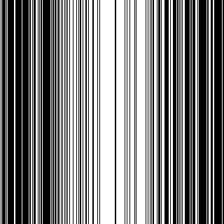
Fig. 2: Sampling masks used in this study. Brains (top) and knees (bottom). Left to right: R2, R3, R4, R5.

3 Results and Discussion

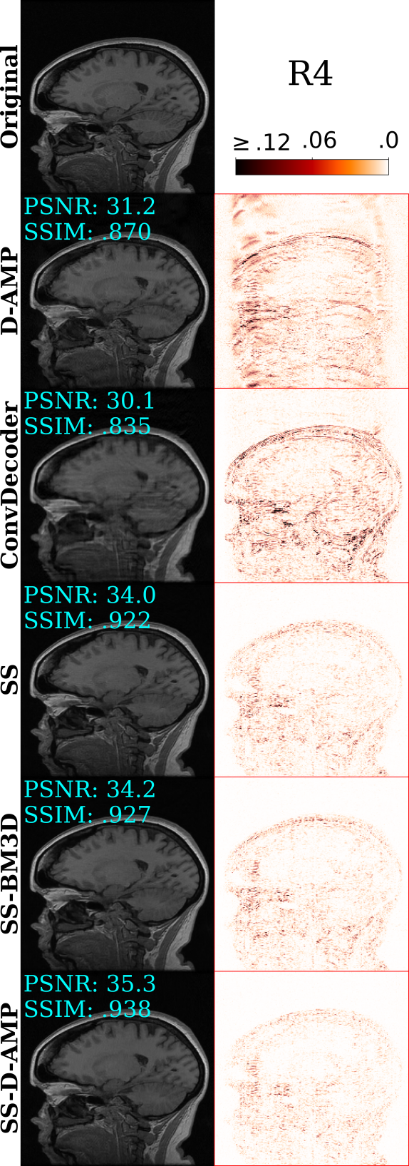
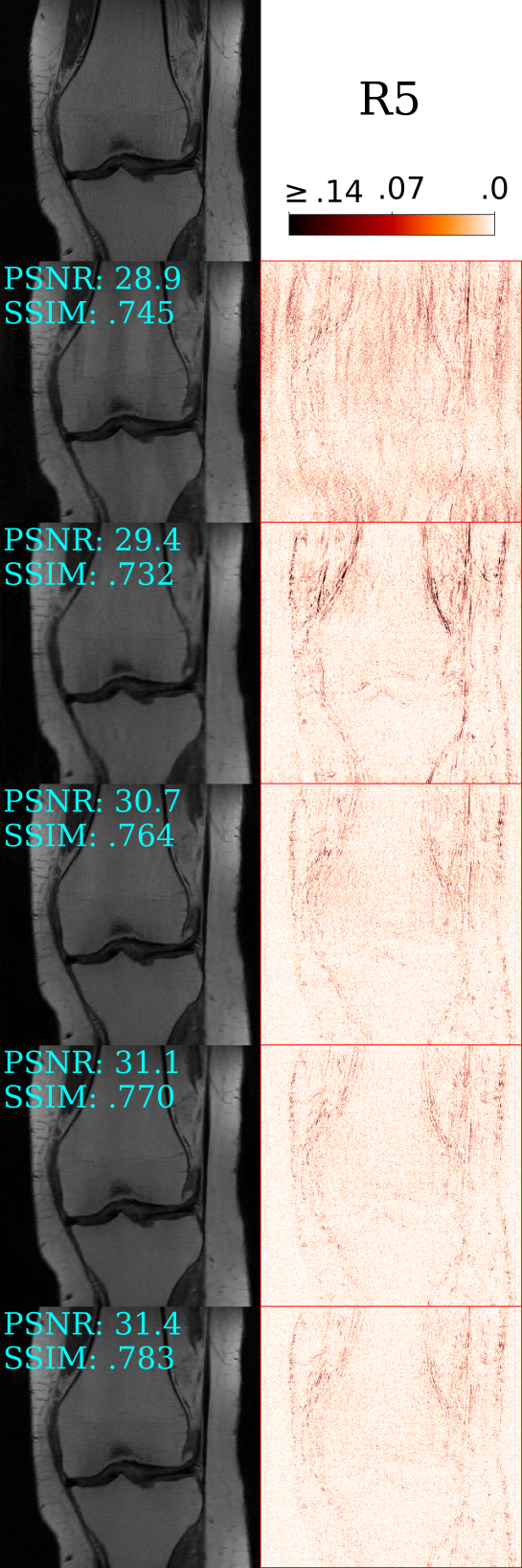
Fig. 3: Representative reconstructions, comparing performance from our SS-based methods on the brain [18] and knee [19] datasets. SS alone is indicative of ZS-SSL [11].

Qualitative Results: Fig. 3 contains a representative comparison between existing single-image techniques D-AMP [2] and ConvDecoder [13] to our proposed approach (best viewed zoomed in). D-AMP does well to remove localised artefacts, however, it struggles with non-local and structured perturbations. ConvDecoder, and to a lesser extent SS, produce localised “ringing” artefacts in the direction of under-sampling. Compared to D-AMP and ConvDecoder, SS effectively penalises non-local and structured CS artefacts, with SS-BM3D scoring higher in terms of PSNR and SSIM (reflected in the error map). Though, SS-BM3D does not meaningfully dampen ringing artefacts as they are not necessarily noise-like. We find SS-D-AMP features the sharpest images with less visible artefacts and better preserved textures, effectively combining the strengths of D-AMP and SS.

Quantitative Results: Fig. 4 illustrates the test loss convergence characteristics of a representative brain reconstruction. Blue is SS, where only Eq. 6 is used for training (similar to ZS-SSL [11]). Orange is SS-BM3D and green is SS-D-AMP, each replacing $g(\cdot)$ with BM3D and D-AMP respectively. While SS-BM3D’s constant denoising (every $30$ epochs) gradually improves the reconstruction compared to SS, denoiser estimates for SS-D-AMP are only completed every $1000$ epochs. In the location of the red arrows, it can be seen that SS-D-AMP noticeably reduces variation between epochs and allows the overall image estimate to improve by $1.5$dB compared to SS. This is because D-AMP regularises $\hat{\mathbf{x}}_{\_}\Omega$ in a manner that ensures CS artefacts are removed without over-smoothing [2]. As a result, $f(\cdot|\Theta)$ continues to minimize the $k$-space consistency loss, whilst ensuring $\mathbf{x}$ does not diverge from the CS estimate.

Table 2 contains the average performance achieved on the 70 brain and 70 knee test slices. SS-D-AMP scores highest overall, improving upon D-AMP by an average 4.49dB and 2.63dB for brains and knees respectively. The main penalty to SS-D-AMP is the increased computation compared to D-AMP and SS. However, Fig. 4 indicates that the SS-D-AMP estimate at epoch $2100$ would produce an image with superior image quality compared to SS or SS-BM3D, enabling a reduction in run-time. Further, SS-BM3D’s non-adaptive Gaussian denoising is less efficient at dampening CS-MRI artefacts than SS-D-AMP, requiring more computation time overall. As ConvDecoder is limited to the mapping of a random vector $\mathbf{z}$ to known measurements $\mathbf{y}_{\_}\Omega$, the reconstruction sees some overfitting and scores lowest on the brains.

Table 2: Average performance achieved by each reconstruction method per dataset. PSNR (dB) SSIM (%).

Method	R=2		R=3		R=4		R=5		s/
	PSNR	SSIM	PSNR	SSIM	PSNR	SSIM	PSNR	SSIM	img
Brains
Zero-Fill	28.10	0.784	25.89	0.720	25.34	0.689	24.81	0.672	-
D-AMP	38.74	0.971	32.29	0.904	31.06	0.874	30.50	0.861	68
ConvDec	35.93	0.941	32.14	0.888	30.28	0.845	29.58	0.836	130
SS	42.56	0.983	37.08	0.957	34.17	0.927	32.45	0.907	209
SS-BM3D	42.68	0.983	37.15	0.958	34.15	0.931	32.34	0.912	329
SS-D-AMP	43.72	0.986	38.25	0.965	35.24	0.941	33.34	0.921	275
Knees
Zero-Fill	27.74	0.778	27.00	0.719	27.87	0.706	26.34	0.658	-
D-AMP	30.53	0.849	30.07	0.804	30.60	0.781	29.29	0.746	78
ConvDec	33.15	0.860	31.53	0.798	30.92	0.760	29.71	0.724	190
SS	34.51	0.880	32.74	0.821	31.74	0.777	30.93	0.748	232
SS-BM3D	34.52	0.881	32.79	0.822	31.79	0.778	31.02	0.750	300
SS-D-AMP	34.65	0.884	32.97	0.829	32.04	0.792	31.33	0.767	254

Fig. 4: Representative test loss. Continuously randomizing $\Lambda,\Upsilon$ helps avoid overfitting. SS-D-AMP improves upon SS by stabilising epoch-to-epoch variations and incorporating the D-AMP reconstruction into the loss function (shown by red arrows).

4 Discussion and Conclusion

Hand-crafted CS-MRI algorithms provide reliable and robust solutions to the image recovery problem. However, DL has emerged as a promising direction due to its ability to produce state-of-the-art images. Unfortunately, DL typically requires large datasets to train satisfactory solutions. Additionally, generalisability across multiple datasets is not guaranteed. Alternatively, single image SS-DL techniques such as ZS-SSL are capable of high-quality image recovery by leveraging the relationship between captured data and the image degradation model. However, reliance on the inherent bias of CNN to produce noise-free images is prone to over-fitting [11]. Recognising that desirable image characteristics are embedded into hand-crafted algorithms, this work develops a SS-CS-MRI paradigm that successfully combines CS algorithms with DL to ensure the solution adheres to well-established image requirements (such as image sparsity). Our findings suggest that this deep and sparse reconstruction is well suited to CS-MRI, outperforming traditional hand-crafted and single image SS-DL techniques. Future work should consider integrating other domain knowledge into the reconstruction procedure, such as leveraging redundancies in multi-coil data (i.e. low-rank). Additionally, inference time can be improved via GPU implementations of D-AMP and BM3D; due to the plug-and-play (PnP) nature of our approach, $g(\cdot)$ can also be replaced by pre-trained DL-CS or Gaussian denoisers. As demonstrated in [13, 11], pre-trained weights $\Theta$ could also be fine-tuned on a single image using our SS-CS-MRI.

5 Compliance with Ethical Standards

This research study was conducted retrospectively using human subject data made available in open access by [18, 19]. Ethical approval was not required as confirmed by the license attached with the open access data.

References

- [1] Michael Lustig, David Donoho, and John M. Pauly, “Sparse MRI: The application of compressed sensing for rapid MR imaging,” Magnetic Resonance in Medicine, vol. 58, no. 6, pp. 1182–1195, 2007.
- [2] Christopher A. Metzler, Arian Maleki, and Richard G. Baraniuk, “From Denoising to Compressed Sensing,” IEEE Transactions on Information Theory, vol. 62, no. 9, pp. 5117–5144, Sept. 2016.
- [3] Jong Chul Ye, “Compressed sensing MRI: a review from signal processing perspective,” BMC Biomedical Engineering, vol. 1, no. 1, pp. 8, Dec. 2019.
- [4] Jo Schlemper, Jose Caballero, Joseph V. Hajnal, Anthony Price, and Daniel Rueckert, “A Deep Cascade of Convolutional Neural Networks for MR Image Reconstruction,” in Information Processing in Medical Imaging, Marc Niethammer, Martin Styner, Stephen Aylward, Hongtu Zhu, Ipek Oguz, Pew-Thian Yap, and Dinggang Shen, Eds., Cham, 2017, Lecture Notes in Computer Science, pp. 647–658, Springer International Publishing.
- [5] Shekhar S Chandra, Marlon Bran Lorenzana, Xinwen Liu, Siyu Liu, Steffen Bollmann, and Stuart Crozier, “Deep learning in magnetic resonance image reconstruction,” Journal of Medical Imaging and Radiation Oncology, vol. 65, no. 5, pp. 564–577, 2021.
- [6] Marlon Bran Lorenzana, Shekhar S. Chandra, and Feng Liu, “AliasNet: Alias artefact suppression network for accelerated phase-encode MRI,” Magnetic Resonance Imaging, vol. 105, pp. 17–28, 2024.
- [7] Burhaneddin Yaman, Seyed Amir Hossein Hosseini, Steen Moeller, Jutta Ellermann, Kâmil Uğurbil, and Mehmet Akçakaya, “Self-supervised learning of physics-guided reconstruction neural networks without fully sampled reference data,” Magnetic Resonance in Medicine, vol. 84, no. 6, pp. 3172–3191, 2020.
- [8] Gushan Zeng, Yi Guo, Jiaying Zhan, Zi Wang, Zongying Lai, Xiaofeng Du, Xiaobo Qu, and Di Guo, “A review on deep learning MRI reconstruction without fully sampled k-space,” BMC Medical Imaging, vol. 21, no. 1, pp. 195, Dec. 2021.
- [9] Chen Hu, Cheng Li, Haifeng Wang, Qiegen Liu, Hairong Zheng, and Shanshan Wang, “Self-supervised Learning for MRI Reconstruction with a Parallel Network Training Framework,” in Medical Image Computing and Computer Assisted Intervention – MICCAI 2021, Marleen de Bruijne, Philippe C. Cattin, Stéphane Cotin, Nicolas Padoy, Stefanie Speidel, Yefeng Zheng, and Caroline Essert, Eds., Cham, 2021, Lecture Notes in Computer Science, pp. 382–391, Springer International Publishing.
- [10] Bo Zhou, Jo Schlemper, Neel Dey, Seyed Sadegh Mohseni Salehi, Kevin Sheth, Chi Liu, James S. Duncan, and Michal Sofka, “Dual-domain self-supervised learning for accelerated non-Cartesian MRI reconstruction,” Medical Image Analysis, vol. 81, pp. 102538, Oct. 2022.
- [11] Burhaneddin Yaman, Seyed Amir Hossein Hosseini, and Mehmet Akcakaya, “Zero-Shot Self-Supervised Learning for MRI Reconstruction,” in International Conference on Learning Representations, 2022.
- [12] Dmitry Ulyanov, Andrea Vedaldi, and Victor Lempitsky, “Deep Image Prior,” 2018, pp. 9446–9454.
- [13] Mohammad Zalbagi Darestani and Reinhard Heckel, “Accelerated MRI With Un-Trained Neural Networks,” IEEE Transactions on Computational Imaging, vol. 7, pp. 724–733, 2021.
- [14] Yuhui Quan, Mingqin Chen, Tongyao Pang, and Hui Ji, “Self2self with dropout: Learning self-supervised denoising from single image,” in 2020 IEEE/CVF Conference on Computer Vision and Pattern Recognition (CVPR), 2020, pp. 1887–1895.
- [15] Gary Mataev, Peyman Milanfar, and Michael Elad, “DeepRED: Deep Image Prior Powered by RED,” 2019, pp. 0–0.
- [16] Yaniv Romano, Michael Elad, and Peyman Milanfar, “The Little Engine That Could: Regularization by Denoising (RED),” SIAM Journal on Imaging Sciences, vol. 10, no. 4, pp. 1804–1844, 2017.
- [17] D.L. Donoho, “Compressed sensing,” IEEE Transactions on Information Theory, vol. 52, no. 4, pp. 1289–1306, 2006.
- [18] Roberto Souza, Oeslle Lucena, Julia Garrafa, David Gobbi, Marina Saluzzi, Simone Appenzeller, Letícia Rittner, Richard Frayne, and Roberto Lotufo, “An open, multi-vendor, multi-field-strength brain MR dataset and analysis of publicly available skull stripping methods agreement,” NeuroImage, vol. 170, pp. 482–494, Apr. 2018.
- [19] Florian Knoll, Jure Zbontar, Anuroop Sriram, Matthew J. Muckley, Mary Bruno, Aaron Defazio, Marc Parente, Krzysztof J. Geras, Joe Katsnelson, Hersh Chandarana, Zizhao Zhang, Michal Drozdzalv, Adriana Romero, Michael Rabbat, Pascal Vincent, James Pinkerton, Duo Wang, Nafissa Yakubova, Erich Owens, C. Lawrence Zitnick, Michael P. Recht, Daniel K. Sodickson, and Yvonne W. Lui, “fastMRI: A Publicly Available Raw k-Space and DICOM Dataset of Knee Images for Accelerated MR Image Reconstruction Using Machine Learning,” Radiology: Artificial Intelligence, vol. 2, no. 1, pp. e190007, Jan. 2020.