Effect of rainbow function on the structural properties of dark energy star

Abstract

Confirming the existence of compact objects with a mass greater than $2.5M_{\odot}$ by observational results such as GW190814 makes that is possible to provide theories to justify these observational results using modified gravity. This motivates us to use gravity’s rainbow, which is the appropriate case for dense objects, to investigate the dark energy star structure as a suggested alternative case to the mass gap between neutron stars and black holes in the perspective of quantum gravity. Hence, in the present work, we derive the modified hydrostatic equilibrium equation for an anisotropic fluid, represented by the extended Chaplygin equation of state in gravity’s rainbow. Then, for two isotropic and anisotropic cases, using the numerical solution, we obtain energy-dependent maximum mass and its corresponding radius, and the other properties of the dark energy star including the pressure, energy density, stability, etc. In the following, using the observational data, we compare the obtained results in two frameworks of general relativity and gravity’s rainbow.

I Introduction

Although until now, by performing various observations, it is possible to state the mass-radius relation and other properties of compact objects, the main problem is determining the equation of state (EOS) governing the inner fluid of the star, because we are not able to correctly determine its nature. The recent accelerating expansion of the universe suggests the existence of a cosmic fluid called dark energy, which is anti-gravitational Peebles2003 . In the structure of compact objects, the EOS of dark energy can also be used as a definition of the inner fluid. The advantage of this choice is that the singularity in the center is avoided. Various stellar models such as false vacuum bubbles Coleman1980 , non-singular black hole Dymnikova1992 , and gravastar Mazur2004 were presented, each of them used different types of dark energy models in the star structure. But the concept of a dark energy star (DES) was first presented by Chapline Chapline assuming the formation of dark energy under a quantum phase transition within the star, visualized a compact object with a quantum critical surface and a singularity-free center. In the following, the stability of this compact object was studied in the presence of anisotropy with the equation of state $p=\omega\rho$ lobo2006 . This EOS with negative dark energy parameter $\omega$ creates pressure against the gravity to prevent the gravitational collapse. By using this EOS, several studies Yazadjiev2011 ; Bhar2015 ; Bhar2018 ; Beltracchi2019 ; Banerjee2020 ; Sakti2021 about dark energy stars and their properties such as pressure behavior, energy density, gravitational profile, and anisotropy were conducted in the last two decades. However, the interest has moved towards the mixed EOSs, which describe the inner behavior of a DES in the presence of dark energy plus various matters. By combining dark energy and ideal Fermi gas, Ghezzi Ghezzi presented a model for the EOS of a dark energy star, which was able to estimate the maximum mass to about $2M_{\odot}$. An EOS including dark energy and baryonic matter was used in Refs. Rahaman2012 ; Bhar2021 , where was shown in Ref. Bhar2021 that the maximum mass can reach close to $2.5M_{\odot}$. A suitable option to describe the behavior of dark energy is the Chaplygin gas (CG) with EOS $p=-\hat{B}/\rho$, which can mimic the behavior of dark matter at early times and dark energy at late times Kamenshchik2001 ; Zheng2022 . It was shown that by adding a barotropic term to Chaplygin gas EOS, the maximum mass of the dark energy star reaches more than $3M_{\odot}$ Panotopoulos2020 ; Panotopoulos2021 ; Pretel2023 ; Tudeshki2023 . These results can open a new window to the mystery of the mass gap region $(2M_{\odot}-5M_{\odot})$ Abbott2020 ; Ozel between neutron stars (NS) and black holes (BH). This means that dark energy stars can be a candidate for compact objects that fill this mass gap region.

Today, several observational reports of the existence of binary star systems have been obtained, which indicate the existence of a companion whose mass can be placed in this mass gap region. Here, some candidates are GW170817 Abbott2017 with total mass of approx $2.73M_{\odot}$, GW190425 with the mass $3.4M_{\odot}$ Abbott2020L3 , and GW190814 with the mass $2.6M_{\odot}$ Abbott2020L44 . Also, the unseen companion of the binary system with the giant 2MASS J05215658+4359220 with the mass $3.3M_{\odot}$ Thompson2019 , massive object in PSR J2215+5135 with the mass $2.27M_{\odot}$ Linares2018 and MSP J0740+6620 with the mass $2.14M_{\odot}$ Cromartie2019 , are also other possible options. Although it is possible to formulate the structure of stars using observational data in the framework of general relativity (GR), however, due to its problems (for example, explaining the current acceleration of our universe and in high energy regime), modified theories of gravity can also be used for this formulation and, of course, to justify the observational results.

In high-energy physics, and especially where the energy of particles can be considered up to the Planck energy $E_{p}$, we need alternative gravity to determine the effect of high energies on the formulation of the system. DES introduced by Chapline Chapline has a surface that allows quantum phase transitions for spacetime. The particles are present at the surface with high energy, which is transformed into dark energy under this phase transition. The gravity’s rainbow (RG) is a theory that is based on quantum gravity and in the UV frequency (high energy) limit, it causes corrections in the energy-momentum dispersion relation Magueijo 2004 . The consequence of this modification is the dependence of the spacetime on energy, which recreates GR in the low frequency (IR) limit. Energy-dependent rainbow functions in RG can influence some properties of compact objects. In this regard, the thermodynamic properties of BH in RG, such as entropy, temperature, Hawking radiation, and other properties have been investigated in several different studies Galan2006 ; Ling2007 ; Liu2008 ; Leiva2009 ; Ali2014 ; Ali2015 ; Feng2017 ; EslamPanah2018 ; EslamPanah2023 . Also, the thermodynamic properties of charged BHs in dilatonic gravity’s rainbow and their dynamic instability in RG have been studied in Refs. HendiFaizal2016 ; HendiPanahiyan2016 . It was shown that the neutron star structure is dependent on rainbow functions HendiBordbar2016 ; EslamPanahetal2017 . Indeed, the maximum mass and radius of neutron stars depended on rainbow functions. For the DES, it was found that the rainbow functions increase the stable regions Tudeshki2022 . With these interpretations, in this work, we intend to find the maximum mass of the DES by studying the energy-dependent spacetime effects and investigating its other properties under these conditions.

II Field and Modified TOV Equations in RG

In the framework of RG, the modified energy momentum dispersion relation is defined as follows Magueijo 2004

$$E^{2}l^{2}(\varepsilon)-p^{2}h^{2}(\varepsilon)=m^{2},$$ (1)

where $\varepsilon=E/E_{P}$ is the ratio of energy $E$ of a particle with mass $m$ to the Planck energy $E_{P}$. Also, $l(\varepsilon)$ and $h(\varepsilon)$ refer to rainbow functions that depend on energy. The rainbow functions must equal unit whenever $\varepsilon$ tends to zero, i.e., $\underset{\varepsilon\longrightarrow 0}{\lim}l(\varepsilon)=1$, and $\underset{\varepsilon\longrightarrow 0}{\lim}h(\varepsilon)=1$. On energy-dependent spacetime can be obtained in terms of orthonormal frame fields

$$H(\varepsilon)=\eta^{ab}e_{a}(\varepsilon)\otimes e_{b}(\varepsilon).$$ (2)

So, the energy-dependent linear element of a static spherical symmetric spacetime in $(3+1)$ dimensions is given

$$ds^{2}=-\frac{e^{2\nu\left(r\right)}}{l^{2}\left(\varepsilon\right)}dt^{2}+\frac{e^{2\lambda\left(r\right)}}{h^{2}\left(\varepsilon\right)}dr^{2}+\frac{r^{2}}{h^{2}\left(\varepsilon\right)}\left(d\theta^{2}+\sin^{2}\theta d\varphi^{2}\right),$$ (3)

where the metric potentials $e^{2\nu\left(r\right)}$ and $e^{2\lambda\left(r\right)}$ have radial-dependent. In RG, the equations of motion are given as follows

$$G_{ab}(\varepsilon)=\dfrac{8\pi G(\varepsilon)}{c(\varepsilon)^{4}}T_{ab}\left(\varepsilon\right),$$ (4)

where $G_{ab}(\varepsilon)$ refers to energy-dependent Einstein’s tensor. Also, $G(\varepsilon)$ is an energy-dependent Newton’s constant. This energy-dependent of $G(\varepsilon)$ indicates that the effective gravitational coupling depends on the energy and confirms a normalization group equation Magueijo 2004 . Besides, $c(\varepsilon)$ is the energy-dependent speed of light. Anyway, here we consider $G(\varepsilon)=c(\varepsilon)=1$. The stress-energy tensor $T_{ab}\left(\varepsilon\right)$ acts as an energy-dependent source. We consider that the interior of the star is filled with an anisotropic fluid. The energy-momentum tensor for an anisotropic distribution $T_{ab}$, is applied according to the following definition Bayin1986

$$T_{ab}\left(\varepsilon\right)=\left[\rho\left(r\right)+p_{t}\left(r\right)\right]u_{a}u_{b}+p_{t}\left(r\right)g_{ab}+\left[p_{r}\left(r\right)-p_{t}\left(r\right)\right]x_{a}x_{b},$$ (5)

where $\rho$ is the energy density. Also, $p_{r}$, and $p_{t}$ are the radial pressure and the transverse pressure, respectively. The four-velocity vector $u_{a}$ applies to normalization relation $u_{a}u^{a}=-1$, and it is obtained from relation $u^{a}=l(\varepsilon)e^{-\nu(r)}\delta_{0}^{a}$. The unit spacelike vector $x_{a}$ also is normalized by $x_{a}x^{a}=1$, and it is determined by $x^{a}=h(\varepsilon)e^{-\lambda(r)}\delta_{1}^{a}$. By substituting the metric in Eq. (5), the mixed diagonal elements of the energy-momentum tensor are determined

$$T_{a}^{b}=diag\left[-\rho\left(r\right),p_{r}\left(r\right),p_{t}\left(r\right),p_{t}\left(r\right)\right].$$ (6)

To obtain the equations of motion, we put Eq. (6) in Eqs. (4). Therefore, the equations of motion are obtained in their extended form in terms of rainbow functions,

$$\dfrac{h^{2}(\varepsilon)(2r\lambda^{\prime}e^{-2\lambda}-e^{-2\lambda}+1)}{r^{2}}=8\pi\rho,$$ (7)

$$\dfrac{h^{2}(\varepsilon)(2r\nu^{\prime}e^{-2\lambda}+e^{-2\lambda}-1)}{r^{2}}=8\pi p_{r},$$ (8)

$$h^{2}(\varepsilon)\left[\nu^{\prime\prime}-\lambda^{\prime}\nu^{\prime}+\nu^{\prime 2}-\frac{\lambda^{\prime}}{r}+\frac{\nu^{\prime}}{r}\right]e^{-2\lambda}=8\pi p_{t},$$ (9)

where the prime and double prime display the first and second derivatives with respect to $r$, respectively.

The ”$tt$” component of the field equations, Eq. (7), gives the following relation

$$e^{-2\lambda}=1-\dfrac{2M_{eff}\left(r,\varepsilon\right)}{r},$$ (10)

in which $M_{eff}\left(r,\varepsilon\right)=\int\limits_{0}^{r}\frac{4\pi r^{\prime 2}\rho dr^{\prime}}{h^{2}\left(\varepsilon\right)}=\frac{m\left(r\right)}{h^{2}\left(\varepsilon\right)}$. It is notable that $M_{eff}\left(r,\varepsilon\right)$ represents the mass-energy function in the RG, and it is known as effective mass, and also $m\left(r\right)$ refers to the mass-energy function in the GR. According to the ”$rr$” component of the field equations (8), the gravity profile is obtained,

$$\frac{d\nu}{dr}=\frac{M_{eff}\left(r,\varepsilon\right)h^{2}\left(\varepsilon\right)+4\pi r^{3}p_{r}}{r\left(r-2M_{eff}\left(r,\varepsilon\right)\right)h^{2}\left(\varepsilon\right)}.$$ (11)

By inserting Eq. (11) into the conservation relation $\triangledown^{a}T_{ab}=0$, and doing some calculations, the modified hydrostatic equilibrium equation (which is known as modified TOV equation) for an anisotropic fluid in the RG is determined Tudeshki2022 ,

$$\frac{dp_{r}}{dr}=-\frac{\left(4\pi r^{3}p_{r}+h^{2}\left(\varepsilon\right)M_{eff}\left(r,\varepsilon\right)\right)\left[p_{r}+\rho\right]}{r\left(r-2M_{eff}\left(r,\varepsilon\right)\right)h^{2}\left(\varepsilon\right)}+\frac{2\left[p_{t}-p_{r}\right]}{r}.$$ (12)

It should be noted that for $h(\varepsilon)=1$, the modified TOV equation (Eq. (12)) reduces to the TOV equation in GR Tolman1939 ; Oppenheimer1939 .

There are various phenomenological motivations for choosing rainbow functions $l(\varepsilon)$ and $h(\varepsilon)$. These functions are mainly divided into three categories, depending on $\varepsilon$. One is based on the loop quantum gravity theory Jacob2010 ; Amelino2013 in the form of $l(\varepsilon)=1$ and $h(\varepsilon)=\sqrt{1-\eta\varepsilon^{n}}$. The other is based on the hard spectra from gamma-ray bursts Amelino1998 as $l(\varepsilon)=\dfrac{e^{\beta\varepsilon}-1}{\beta\varepsilon}$ and $h(\varepsilon)=1$. Another option that we are interested to use in this study for rainbow functions, is to ensure that the speed of light does not change Magueijo 2002 , which is defined $l(\varepsilon)=h(\varepsilon)=\frac{1}{1-\psi\varepsilon}$. Above, $\eta$, $\beta$, and $\psi$ are parameters determined by empirical methods. Due to the positive assumption of rainbow functions, $\psi$ applies in $\psi<\dfrac{1}{\varepsilon}$. On the other hand, the maximum energy assumed for a particle cannot exceed the Planck energy limit. So it must be $\varepsilon<1$. As a result, rainbow functions assume positive values greater than unity, and they become $1$ in the IR limit (or for GR).

III Properties of DESs in RG and Observational Data

EOS and Anisotropy Model: In order to characterize the internal behavior of the DES, an appropriate EOS must be considered. As a suitable candidate for dark energy that is consistent with the observational results such as CMB data, supernova data, etc., we can mention the generalized Chaplygin gas (GCG) model, which is known as a cosmic fluid and has an EOS; $p_{r}=-\hat{B}/\rho^{\omega}$ Gorini2003 ; Xu2012 , where $\hat{B}$ is a constant with units of [length^-4], and also $\omega$ is a constant in the range of $0\leq\omega\leq 1$. By adding a barotropic term to GCG EOS, the modified Chaplygin gas (MCG) EOS is defined as follows Debnath2004 ; Benaoum2012 ; Mazumder2012 ,

$$p_{r}=\hat{A}\rho-\frac{\hat{B}}{\rho^{\omega}},$$ (13)

where the constant dimensionless values of $\hat{A}$ are determined from the considerations of establishing the causality condition at the star surface. The above equation can be written in the following form Panotopoulos2020 ; Panotopoulos2021 ,

$$p_{r}=A^{2}\rho-\dfrac{B^{2}}{\rho}.$$ (14)

Here $\omega=1$ is assumed. The square of sound speed should be less than $1$, i.e., $0<V_{sr}^{2}=\dfrac{dp_{r}}{d\rho}=A^{2}+B^{2}/\rho^{2}<1$, because the sound speed should be less than the speed of light. So the causality condition must be satisfied. On the other hand, at the surface of star $(r=R)$, the radial pressure is neglected, so the energy density and constants $A$ and $B$ apply in the relation $B=A\rho$. As a result, the causality condition is obeyed by $V_{sr}^{2}(R)=2A^{2}<1$. It is clear that ${A}$ must be less than $\sqrt{0.5}$ and $B$ is determined using values of $A$ Pretel2023 ; Tudeshki2023 . According to above discussions, in this paper, we use the extended Chaplygin EOS (14) to make a comparison with the previous studies Panotopoulos2020 ; Panotopoulos2021 ; Tudeshki2023 , where values $A=\sqrt{0.4}$ and $B=0.2\times 10^{-3}km^{-2}$ are included in the numerical solution.

One of the unknown quantities in the hydrostatic equilibrium equation is the anisotropy factor $\Delta$, which includes radial and transverse pressures in the form of $p_{t}-p_{r}$. In examining more realistic models of stars, it has been shown that in densities greater than nuclear density, in addition to radial pressure inside the star, transverse pressure is also created perpendicular to radial direction Ruderman ; Canuto . In addition, the occurrence of physical phenomena such as phase transition Sokolov , condensation Hartle and electromagnetic fields Usov ; bordbar2022 are also effective in creating anisotropy. In some studies Bowers1974 ; Cosenza1981 ; Horvat2010 ; Doneva2012 ; Herrera2013 ; Raposo2019 , several models have been presented to describe the behavior of the anisotropy factor. Here, inspired by the nonlinear model presented by Bowers and Liang Bowers1974 (called BL anisotropic model), we define a modified version of this model in the RG, which is as follows,

$$\Delta=p_{t}-p_{r}=\dfrac{\Upsilon\left(\rho+3p_{r}\right)\left(\rho+p_{r}\right)r^{2}}{1-\frac{2M_{eff}\left(r,\varepsilon\right)}{r}},$$ (15)

where $\Upsilon$ is a constant determining the degree of anisotropy. $\Upsilon$ must be less than $2/3$ to satisfy condition $(M_{eff}/R)_{critical}>0$ Bowers1974 .

Numerical Solutions: The numerical solution of three coupled differential equations (11), (12), and effective mass for two cases $\Upsilon=0$ and $\Upsilon\neq 0$ leads to the determination of the properties of DESs in RG with two isotropic and anisotropic configurations, respectively. Numerical solution is made by considering the following initial conditions at the center of the star, $M_{eff}(r=0)=0$, and $\rho(r=0)=\rho_{c}$. Also, the boundary condition on the surface $p_{r}(R)=0$, in addition to $M(R)=M_{eff}(r=R)$, and $\nu(R)=\dfrac{1}{2}ln\left(1-2M(R)/R\right)$, where $\rho_{c}$ is the central energy density, $M(R)$ is the total mass of DES in RG and $\nu(R)$ is related to metric potentials at radius $R$. It should be noted that conditions $\Delta(r=0)=0$ and $\rho_{s}=B/A$ are also met. In the following, the results for the central density $\rho_{c}=1.35\times 10^{15}~{}g/cm^{3}$ and different values of the rainbow function $h(\varepsilon)$ are specified in Tables 1 and 2 for isotropic and anisotropic fluid. Also, for a range of central energy density, the maximum mass and its corresponding radius are obtained.

Table 1: The properties of isotropic DES in RG with $A=\sqrt{0.4}$, $B=0.2\times 10^{-3}$ and different values of $h(\varepsilon)$.

$h(\varepsilon)$	$M_{max}[M_{{}_{\odot}}]$	$R[km]$	$R_{Sch}[km]$	$\sigma$	$Z_{s}$
$1$	$2.64$	$12.63$	$7.83$	$0.30$	$0.61$
$1.15$	$3.04$	$14.53$	$9.00$	$0.30$	$0.61$
$1.20$	$3.17$	$15.16$	$9.39$	$0.30$	$0.61$
$1.25$	$3.31$	$15.79$	$9.78$	$0.30$	$0.61$
$1.30$	$3.44$	$16.42$	$10.18$	$0.30$	$0.61$
$1.35$	$3.57$	$17.06$	$10.57$	$0.30$	$0.61$
$1.40$	$3.70$	$17.69$	$10.96$	$0.30$	$0.61$

Table 2: The properties of anisotropic DES in RG with $A=\sqrt{0.4}$, $B=0.23\times 10^{-3}$, $\Upsilon=0.1$ and different values of $h(\varepsilon)$.

$h(\varepsilon)$	$M_{max}[M_{{}_{\odot}}]$	$R[km]$	$R_{Sch}[km]$	$\Delta_{s}[dyn/cm^{2}]$	$\sigma$	$Z_{s}$
$1$	$2.72$	$12.83$	$8.07$	$5.37\times 10^{33}$	$0.31$	$0.64$
$1.15$	$3.16$	$14.80$	$9.38$	$7.24\times 10^{33}$	$0.31$	$0.65$
$1.2$	$3.19$	$15.46$	$9.82$	$7.93\times 10^{33}$	$0.31$	$0.65$
$1.25$	$3.47$	$16.12$	$10.27$	$8.67\times 10^{33}$	$0.31$	$0.65$
$1.3$	$3.62$	$16.78$	$10.72$	$9.44\times 10^{33}$	$0.31$	$0.66$
$1.35$	$3.77$	$17.45$	$11.18$	$1.02\times 10^{34}$	$0.32$	$0.66$
$1.4$	$3.93$	$18.11$	$11.64$	$1.11\times 10^{34}$	$0.32$	$0.67$

Pressure, Density and Anisotropy Factor: The behaviors of density and radial pressure versus distance are plotted in Fig. 1. As one can see, the density (pressure) in the center of DES has the maximum value. As it moves toward the surface of DES, it finds a downward trend, and finally reaches its minimum value at the surface. Increasing the rainbow function $h(\varepsilon)$ at a certain density results in increasing the radius.

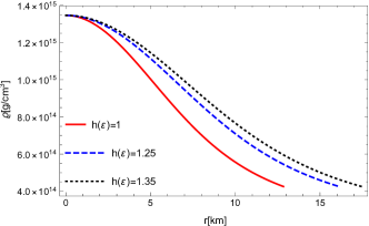
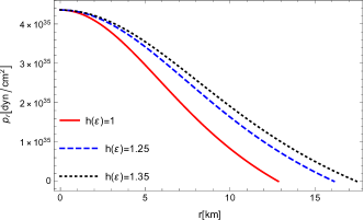
Figure 1: Density $\varrho$ vs radius $r$ (left panel) and radial pressure $p_{r}$ vs radius $r$ for different $h(\varepsilon)$ (right panel) with $\Upsilon=0.1$, $A=\sqrt{0.4}$ and $B=0.2\times 10^{-3}$.

Fig. 2 shows the anisotropy factor $\Delta$ versus radius. In the left panel of Fig. 2, we see that by increasing the value of rainbow function $h(\varepsilon)$, the $\Delta$ value has also increased. In the right panel of Fig. 2, it can be seen that the $\Delta$ increases by increasing the degree of anisotropy $\Upsilon$. Note that in the center of the star $\Delta=0$, because $p_{t}(r=0)=p_{r}(r=0)$.

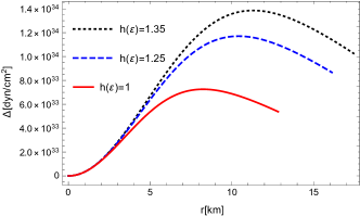
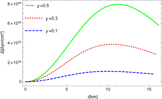
Figure 2: Anisotropy factor ($\Delta$) vs radius $r$ for $\Upsilon=0.1$ and different $h(\varepsilon)$ (left panel). For $h(\varepsilon)=1.20$, $A=\sqrt{0.4}$, $B=0.2\times 10^{-3}$ and different $\Upsilon$ (right panel).

Maximum Mass and its Corresponding Radius: There are Several reasons to make the maximum mass calculated for compact objects such as neutron stars approaches the result obtained from the GW190814 event $(M_{max}>2.5M_{\odot})$, including the presence of dense matter with different EOSs. It has also shown that the presence of anisotropy is also able to increase the maximum mass in a DES Pretel2023 . However, due to the unknown nature of dark energy, various EOSs with free parameters are consistent with observational results, capable of predicting the mass range region of DES Panotopoulos2020 ; Panotopoulos2021 . The results have shown that in addition to the fact that the maximum mass calculated for the DES is within the mass range obtained for the neutron stars, it is even capable of justifying the mass gap region between the massive neutron star and the low-mass black hole $2M_{\odot}-5M_{\odot}$ Abbott2020 ; Ozel ; Thompson2019 . Despite the study on the structure of compact stars with dark energy in GR Haghani , however, DESs have been studied in modified gravity such as massive gravity and suggested a maximum mass of more than $3M_{\odot}$ Tudeshki2023 . Motivated by the effect of high-energy limit (UV limit) on compact objects such as DES, in present work, we investigate the effect of the energy-dependent rainbow function $h(\varepsilon)$ on the maximum mass $M_{max}$ and its corresponding radius $R$ for two cases of isotropic and anisotropic fluid using a numerical solution. Since we intend to study the role of RG and the anisotropy parameter $\Upsilon$ on the behavior of the maximum mass $M_{max}$ of DES, we fix other involved parameters, including the parameters of EOS $A$ and $B$.

Mass-radius relation diagrams in Fig. 3 contain colored bands, where each of them represents the mass range of observational candidates, which are introduced in the caption below the diagram. According to the upper panel in Fig. 3, the curve related to isotropic GR passes through all color bands, and its maximum reaches that of GW190814. But other curves related to isotropic RG, with the increase of the rainbow function $h(\varepsilon)$ up to $1.35$ also exceed the limit of GW190814, and the maximum mass reaches the value of $3.7M_{\odot}$. In the middle panel in Fig. 3, the anisotropic GR curve is slightly above the limit of GW190814. Also, in other curves, the maxima in RG increase with the presence of $\Upsilon$ and reach the highest value in $3.9M_{\odot}$. With a look at the bottom panel of Fig. 3, one can see that although GR covers the observational data range NS pulsars (J1614-2230 and J0348+0432), NS pulsars J0740+6620 and J2215+5135 and also GW190814, but compared to RG, it is not able to cover the areas above the gray band. These regions include mass range 2MASS J05215658+4359220 and GW190425 with values $3.3M_{\odot}$ and $3.4M_{\odot}$, respectively, which are satisfied only in RG (For simplicity, observational data J05215658+4359220 and GW190425 are not included in the plot). An interesting point is that even if we increase the degree of anisotropy of the model in GR, the anisotropic RG model provides us with larger values of the maximum mass. At the end of this part, we display the agreement of the results obtained for the RG and GR frameworks with the data of different observational candidates in Table. 3. It should be noted that this comparison is made for the fixed values $A=\sqrt{0.4}$, $B=0.2\times 10^{-3}$, and $\Upsilon=0.1$.

Table 3: Different observational data and agreement with the calculation results of Chaplygin EOS between general relativity (GR) and gravity’s rainbow (RG). It is notable that the abbreviations of ”iso” and ”ani” are related to the isotropic and anisotropic, respectively.

Observational	GR	GR	RG	RG
candidate	(iso)	(ani)	(iso)	(ani)
GW190814	$\checkmark$	$\checkmark$	$\checkmark$	$\checkmark$
GW170817	$\checkmark$	$\checkmark$	$\checkmark$	$\checkmark$
GW190425	$\times$	$\times$	$\checkmark$	$\checkmark$
J05215658+4359220	$\times$	$\times$	$\checkmark$	$\checkmark$
PSR J1614-2230	$\checkmark$	$\checkmark$	$\checkmark$	$\checkmark$
PSR J0348+0432	$\checkmark$	$\checkmark$	$\checkmark$	$\checkmark$
PSR J0740+6620	$\checkmark$	$\checkmark$	$\checkmark$	$\checkmark$
PSR J2215+5135	$\checkmark$	$\checkmark$	$\checkmark$	$\checkmark$
PSR J1311-3430	$\checkmark$	$\checkmark$	$\checkmark$	$\checkmark$
PSR J1748-2021B	$\checkmark$	$\checkmark$	$\checkmark$	$\checkmark$

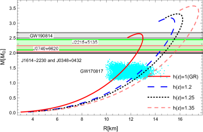
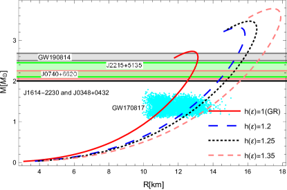
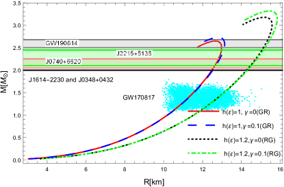
Figure 3: Mass-radius relation. Isotropic model $\Upsilon=0$ (up panel), anisotropic model $\Upsilon\neq 0$ (middle panel) for DES with $A=\sqrt{0.4}$ and $B=0.2\times 10^{-3}$ and different values $h(\varepsilon)$. Comparison of isotropic and anisotropic models in GR and RG (down panel). At $M=2M_{\odot}$, the black horizontal line shows the mass data of the massive NS pulsars (J1614-2230 and J0348+0432). The wide pink and green bars display the observational mass data of NS pulsars J0740+6620 and J2215+5135, respectively. Observational data from event GW190814 has been shown in the gray bar. Also the cyan area shows mass-radius constraints of component binary pair mass-radius constraints (GW170817 event).

Schwarzschild Radius: To calculate the modified Schwarzschild radius $R_{Sch}$ in RG, we must set the metric function (10) equal to zero, i.e., $e^{-2\lambda(r=R_{Sch})}=0$. So, the modified Schwarzschild radius in the RG is obtained HendiFaizal2016 ; HendiPanahiyan2016 ; HendiBordbar2016 ,

$$R_{Sch}=2M_{eff}.$$ (16)

Since the effective mass $M_{eff}$ depends on the rainbow function $h(\varepsilon)$, as a result, $R_{Sch}$ also depends on the energy. According to the results of Tables 1 and 2, we see that by increasing the rainbow function $h(\varepsilon)$, $R_{Sch}$ also increases. Notably, these compact objects cannot be black holes, because their radii are less than Schwarzschild radii ($R>R_{Sch}$).

Compactness: The degree of compactness of a compact object is defined by the ratio of its mass $M$ to its radius $R$. The mass obtained in the gravity’s rainbow is defined in terms of effective mass $M_{eff}$. Therefore, the compactness relation in RG is generalized as follows,

$$\sigma=\dfrac{M_{eff}}{R}.$$ (17)

According to the results of Tables 1 and (2), it can be seen that for different values of the rainbow function $h(\varepsilon)$, the compactness remains almost unchanged in both isotropic and anisotropic models.

Gravitational Redshift: We can obtain the surface gravitational redshift $Z_{s}$ using Eq. (10) and definition $1+Z_{s}=e^{\lambda(R)}$ as follows HendiBordbar2016 ,

$$1+Z_{s}=\dfrac{1}{\sqrt{1-2\sigma}}.$$ (18)

As can be seen from the above relation, surface gravitational redshift is related to compactness. Since the $\sigma$ is approximately fixed for different values of the rainbow function $h(\varepsilon)$, as a result, $Z_{s}$ also has very small changes (see Tables 1, and 2, and also Fig. 4).

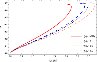
Figure 4: Surface gravitational redshift ($Z_{s}$) vs mass ($M$) in the RG with different $h(\varepsilon)$ for anisotropic model with $A=\sqrt{0.4}$, and $B=0.2\times 10^{-3}$.

Energy Condition: For an anisotropic fluid, the energy conditions are valid if all conditions such as the null energy condition (NEC), weak energy condition (WEC), strong energy condition(SEC), and dominant energy condition (DEC) are satisfied Leon1993 . Using the numerical results obtained for energy density $\rho$, radial pressure $p_{r}$ and anisotropy factor $\Delta=p_{t}-p_{r}$, according to the Table 4, these conditions are briefly categorized, and their validity is evaluated. It can be seen that all the energy conditions are valid in the RG. Although MCG EOS describes the dark energy in this star, the strong energy condition is satisfied, which indicates that the dark energy in this star behaves like matter.

Table 4: Energy conditions of DES in RG with $h(\varepsilon)=1.2$, $A=\sqrt{0.4}$, $\Upsilon=0.1$, and $B=0.2\times 10^{-3}$.

NEC	WEC	SEC	DEC
$\rho+p_{r}\geq 0$	$\rho\geq 0$	$\rho+p_{r}+2p_{t}\geq 0$	$\rho\geq\left|p_{r}\right|$
$\rho+p_{t}\geq 0$	$\rho+p_{r}\geq 0$,  $\rho+p_{t}\geq 0$	$\rho+p_{t}\geq 0$	$\rho\geq\left|p_{t}\right|$
$\checkmark$	$\checkmark$	$\checkmark$	$\checkmark$

IV STABILITY

To check the stability of compact objects, it is customary to use several different tests, which are mentioned below.

IV.1 Causality and Cracking

In models of anisotropic fluid where the fluid has two radial and transverse pressures, the causality condition is valid when two conditions, $0<V_{sr}^{2}=\dfrac{dp_{r}}{d\rho}<1$ and $0<V_{st}^{2}=\dfrac{dp_{t}}{d\rho}<1$ are met Herrera1992 . The quantities $V_{sr}$ and $V_{st}$ are the radial and transverse speeds of sound, respectively. This means that the speed of sound in both radial and transverse directions should not exceed the speed of light. In Fig. (5), $V_{sr}^{2}$ and $V_{st}^{2}$ are plotted versus radius.

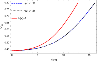
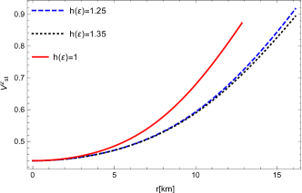
Figure 5: Square of radial speed of sound $V_{sr}^{2}$ (left panel) and square of transverse speed of sound $V_{st}^{2}$ (right panel) vs radius in RG for $A=\sqrt{0.4}$, $B=0.2\times 10^{-3}$, $\Upsilon=0.1$, and different $h(\varepsilon)$.

According to Fig. 5 for different values of $h(\varepsilon)$, the causality condition is still satisfied. Also, an interesting phenomenon occurs in locally anisotropic configurations, known as cracking Herrera1992 ; Abreu2007 . In fact, the ratio of the anisotropy factor perturbations to density perturbations in a fluid creates cracking, which is related to the sound speed in the following form,

$$\dfrac{\delta\Delta}{\delta\rho}\sim\dfrac{\delta(p_{t}-p_{r})}{\delta\rho}\sim\dfrac{\delta p_{t}}{\delta\rho}-\dfrac{\delta p_{r}}{\delta\rho}\sim V_{st}^{2}-V_{sr}^{2}.$$ (19)

This difference in the square of sound speed is a measure that shows the state of stability of the compact object against perturbations caused by anisotropy. Therefore, the following two criteria are used to check the stability under cracking,

$$-1<V_{st}^{2}-V_{sr}^{2}<0~{}~{}~{}\text{potentially~{}stable,}$$ (20)

$$0<V_{st}^{2}-V_{sr}^{2}<1~{}~{}~{}\text{potentially~{}unstable.}$$ (21)

Fig. (6) shows a view of the cracking criteria, i.e., the difference between $V_{st}^{2}-V_{sr}^{2}$ versus the radius. As can be seen, for different values of the rainbow function $h(\varepsilon)$, the curves are in the positive part of the plot, and this means that the system is potentially unstable.

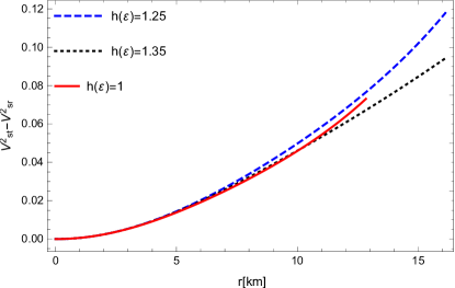
Figure 6: $V_{st}^{2}-V_{sr}^{2}$ vs radius in RG for $A=\sqrt{0.4}$, $B=0.2\times 10^{-3}$, $\Upsilon=0.1$, and different $h(\varepsilon)$.

IV.2 Adiabatic Index

Under the radial perturbations created in an anisotropic fluid, the adiabatic index can be considered as follows Chandrasekhar1964 ; Bondi1964 ; Chan1993 ,

$$\Gamma_{r}=\left(1+\dfrac{\rho}{p_{r}}\right)V_{sr}^{2}.$$ (22)

Although the system is under anisotropy, checking its dynamic stability through the adiabatic index is sufficient for the above relation, because these are radial perturbations. Regions are dynamically stable where the adiabatic index is $\Gamma_{r}>1.33$. In Fig. 7, the adiabatic index curves are drawn for different values of the rainbow function. It can be seen that all values are greater than $1.33$. Therefore, the obtained DESs in the RG are dynamically stable.

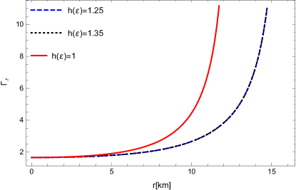
Figure 7: Adiabatic index ($\Gamma_{r}$) vs radius in RG with $A=\sqrt{0.4}$, $B=0.2\times 10^{-3}$, and different $h(\varepsilon)$.

IV.3 Harrison-Zeldovich-Novikov condition

Harrison-Zeldovich-Novikov condition Zeldovich1971 ; Harrison1965 states that a compact object maintains its dynamical stability if it satisfies the condition $dM/d\rho_{c}>0$. This means that as long as this condition is met, the compact object resists gravitational collapse. In Fig. 8, we see that the curves have an ascending trend up to a critical energy density $\rho_{crit}$. Here, our studied system is considered up to $dM/d\rho_{c}=0$, where the critical density is $\rho_{crit}$. As a result, the dark energy star is completely stable in the range $\rho_{c}\leq\rho_{crit}$. After this limit, i.e. $\rho_{c}>\rho_{crit}$, the star becomes unstable, and it may collapse and turn into a black hole.

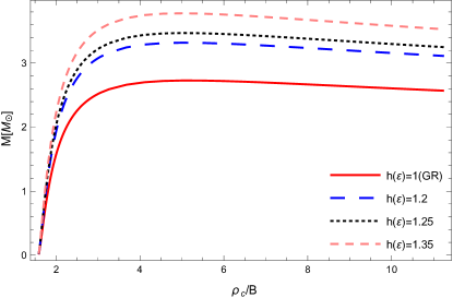
Figure 8: Mass-central energy density relation with anisotropic model $\Upsilon\neq 0$ with $A=\sqrt{0.3}$, $B=0.2\times 10^{-3}$, and different values $h(\varepsilon)$.

V Summary and Conclusions

In summary, in this study, we discussed the possible effects of energy-dependent spacetime on the structure of dark energy star and especially the maximum mass $M_{max}$ and its corresponding radius $R$. For this purpose, we obtained the generalized hydrostatic equilibrium equation in the gravity’s rainbow for an anisotropic fluid by using the extended Chaplygin gas equation of state and Bowers and Liang anisotropy model. Then, using the numerical solutions in two gravitational frameworks, general relativity and gravity’s rainbow, the behavior of physical quantities of the dark energy star such as density, radial pressure and anisotropy, the maximum mass and its corresponding radius, compactness, and gravitational redshift for the different values of the rainbow function $h(\varepsilon)$ were analyzed in two isotropic and anisotropic models.

The obtained results showed that we can make a constraint on the maximum mass of the dark energy star by gravity’s rainbow. This dependence on the energy leads the maximum mass $M_{max}\sim 3.70$ in the isotropic model and the maximum mass $M_{max}\sim 3.90$ in the anisotropic model. These obtained masses are in the mass gap region $2M_{\odot}-5M_{\odot}$, which could be a justification for the existence of observed compact objects similar to the mass observed in two observational candidates GW190425 and J05215658+4359220. We also indicated that, in comparison between gravity’s rainbow and general relativity, gravity’s rainbow could cover a wider range of mass gap regions.

The stability of dark energy star was studied with different tests. It was shown that although the causality condition in the configuration is satisfied, the perturbations due to anisotropy induce a crack in the system, which makes the dark energy star potentially unstable. However, the dark energy star is stable up to a critical limit for the central density. Also due to the increase in central density, the star will be undergo gravitational collapse.

From a general point of view, it can be said that the dependence of spacetime on the energy of particles has a significant effect on the maximum mass of compact objects. Matching these results obtained from our theoretical model with observational evidence will help us to improve our other theoretical models in the future.

- (1) P. J. E. Peebles, and B. Ratra, Rev. Mod. Phys. 75 (2003) 559.
- (2) S. Coleman, and F. De Luccia, Phys. Rev. D 21 (1980) 3305.
- (3) I. Dymnikova, Gen. Relativ. Grav. 24 (1992) 235.
- (4) P. O. Mazur, and E. Mottola, Proc. Nat. Acad. Sci. 101 (2004) 9545.
- (5) G. Chapline, Dark Energy Stars, [arXiv:astro-ph/0503200].
- (6) F. S. Lobo, Class. Quantum Grav. 23 (2006) 1525.
- (7) S. S. Yazadjiev, Phys. Rev. D 83 (2011) 127501.
- (8) P. Bhar, and F. Rahaman, Eur. Phys. J. C 75 (2015) 1.
- (9) P. Bhar, et al., Can. J. Phys. 96 (2018) 594.
- (10) P. Beltracchi, and P. Gondolo, Phys. Rev. D 99 (2019) 044037.
- (11) A. Banerjee, M. Jasim, and A. Pradhan, Mod. Phys. Lett. A 35 (2020) 2050071.
- (12) M. F. A. Rangga Sakti, and A. Sulaksono, Phys. Rev. D 103 (2021) 084042
- (13) C. R. Ghezzi, Astrophys. Space Sci. 333 (2011) 437.
- (14) F. Rahaman, et al., Gen. Relativ. Grav. 44 (2012) 107.
- (15) P. Bhar, Phys. Dark Universe. 34 (2021) 100879.
- (16) A. Kamenshchik, U. Moschella, and V. Pasquier, Phys. Lett. B 511 (2001) 265.
- (17) J. Zheng, et al., Eur. Phys. J. C 82 (2022) 582.
- (18) G. Panotopoulos, A. Rincon, and I. Lopes, Eur. Phys. J. Plus. 135 (2020) 1.
- (19) G. Panotopoulos, A. Rincon, and I. Lopes, Phys. Dark Universe. 34 (2021) 100885.
- (20) J. M. Pretel, Eur. Phys. J. C 83 (2023) 26.
- (21) A. Bagheri Tudeshki, G. H. Bordbar, and B. Eslam Panah, Phys. Dark Universe. 42 (2023) 101354.
- (22) B. P. Abbott, et al., Astrophys. J. Lett. 882 (2019) L24.
- (23) F. Ozel, et al., Astrophys. J. 725 (2010) 1918 .
- (24) B. P. Abbott, et al., Phys. Rev. Lett. 119 (2017) 161101.
- (25) B. P. Abbott, et al., Astrophys. J. Lett. 892 (2020) L3.
- (26) B. P. Abbott, et al., Astrophys. J. Lett. 896 (2020) L44.
- (27) T. A. Thompson, et al., Science. 366 (2019) 637.
- (28) M. Linares, T. Shahbaz, and J. Casares, Astrophys. J. 859 (2018) 54.
- (29) H. T. Cromartie, et al., Nat. Astronomy. 4 (2019) 72.
- (30) J. Magueijo, and L. Smolin, Class. Quantum Grav. 21 (2004) 1725.
- (31) P. Galan, and G. A. Mena Marugan, Phys. Rev. D 74 (2006) 044035.
- (32) Y. Ling, X. Li, and H. Zhang, Mod. Phys. Lett. A 22 (2007) 2749.
- (33) C. Z. Liu, and J. Y. Zhu, Gen. Relativ. Grav. 40 (2008) 1899.
- (34) C. Leiva, J. Saavedra, and J. Villanueva, Mod. Phys. Lett. A 24 (2009) 1443.
- (35) A. F. Ali, Phys. Rev. D 89 (2014) 104040.
- (36) A. F. Ali, M. Faizal, and B. Majumder, Europhys. Lett. 109 (2015) 20001.
- (37) Z. W. Feng, and S. Z. Yang, Phys. Lett. B 772 (2017) 737.
- (38) B. Eslam Panah, Phys. Lett. B 787 (2018) 45.
- (39) B. Eslam Panah, Phys. Lett. B 844 (2023) 139069.
- (40) S. H. Hendi, et al., Eur. Phys. J. C 76 (2016) 296.
- (41) S. H. Hendi, et al., Eur. Phys. J. C 76 (2016) 150.
- (42) S. H. Hendi, et al., JCAP 09 (2016) 013.
- (43) B. Eslam Panah, et al., Astrophys. J. 848 (2017) 24.
- (44) A. Bagheri Tudeshki, G. H. Bordbar, and B. Eslam Panah, Phys. Lett. B 835 (2022) 137523.
- (45) S. S. Bayin, Astrophys. J. 303 (1986) 101.
- (46) R. C. Tolman, Phys. Rev. 55 (1939) 364.
- (47) J. R. Oppenheimer, and G. M. Volkoff, Phys. Rev. 55 (1939) 374.
- (48) U. Jacob et al., Phys. Rev. D 82 (2010) 084021.
- (49) G. Amelino-Camelia, Living Rev. Rel. 5 (2013) 16.
- (50) G. Amelino-Camelia, et al., Nature. 393 (1998) 763.
- (51) J. Magueijo, and L. Smolin, Phys. Rev. Lett. 88 (2002) 190403.
- (52) V. Gorini, A. Kamenshchik, and U. Moschella, Phys. Rev. D 67 (2003) 063509.
- (53) Y. D. Xu, et al., Astrophys. Space Sci. 339 (2012) 31.
- (54) U. Debnath, A. Banerjee, and S. Chakraborty, Class. Quantum Grav. 21 (2004) 5609.
- (55) H. B. Benaoum, Adv. High Energy Phys. 2012 (2012) 357802.
- (56) N. Mazumder, et al., Int. J. Theor. Phys. 51 (2012) 2754.
- (57) M. Ruderman, Annu. Rev. Astron. Astrophys. 10 (1972) 427.
- (58) V. Canuto, and S. M. Chitre, Phys. Rev. D 9 (1974) 1587.
- (59) A. I. Sokolov, J. Exp. Theor. Phys. 52 (1980) 575.
- (60) J. B. Hartle, R. F. Sawyer, and D. J. Scalapino, Astrophys. J. 199 (1975) 471.
- (61) V. V. Usov, Phys. Rev. D 70 (2004) 067301.
- (62) G. H. Bordbar, and M. Karami, Eur. Phys. J. C 82 (2022) 1.
- (63) R. L. Bowers, and E. P. T. Liang, Astrophys. J. 188 (1974) 657.
- (64) M. Cosenza et al., J. Math. Phys. 22 (1981) 118.
- (65) D. Horvat, S. Ilijic, and A. Marunovic, Class. Quantum Grav. 28 (2010) 025009.
- (66) D. D. Doneva, and S. S. Yazadjiev, Phys. Rev. D 85 (2012) 124023.
- (67) L. Herrera, and W. Barreto, Phys. Rev. D 88 (2013) 084022.
- (68) G. Raposo, et al., Phys. Rev. D 99 (2019) 104072.
- (69) Z. Haghani, and T. Harko, Phys. Rev. D 105 (2022) 064059.
- (70) J. Ponce de Leon, Gen. Relativ. Grav. 25 (1993) 1123.
- (71) L. Herrera, Phys. Lett. A 165 (1992) 206.
- (72) H. Abreu, H. Hernandez, and L. A. Nunez, Class. Quantum Grav. 24 (2007) 4631.
- (73) S. Chandrasekhar, Astrophys. J. 140 (1964) 417.
- (74) H. Bondi, Proc. R. Soc. Lond. A 281 (1964) 39.
- (75) R. Chan, L. Herrera, and N. O. Santos, MNRAS 265 (1993) 533.
- (76) Y. B. Zeldovich, and I. D. Novikov, Relativistic astrophysics. Vol.1: Stars and relativity, Chicago: University of Chicago Press (1971).
- (77) B. K. Harrison, K. S. Thorne, M. Wakano, and J. A. Wheeler, Gravitation Theory and Gravitational Collapse, Chicago: University of Chicago Press (1965).