PIE-NeRF: Physics-based Interactive Elastodynamics with NeRF

Abstract

We show that physics-based simulations can be seamlessly integrated with NeRF to generate high-quality elastodynamics of real-world objects. Unlike existing methods, we discretize nonlinear hyperelasticity in a meshless way, obviating the necessity for intermediate auxiliary shape proxies like a tetrahedral mesh or voxel grid. A quadratic generalized moving least square (Q-GMLS) is employed to capture nonlinear dynamics and large deformation on the implicit model. Such meshless integration enables versatile simulations of complex and codimensional shapes. We adaptively place the least-square kernels according to the NeRF density field to significantly reduce the complexity of the nonlinear simulation. As a result, physically realistic animations can be conveniently synthesized using our method for a wide range of hyperelastic materials at an interactive rate. For more information, please visit our project page at https://fytalon.github.io/pienerf/.

1 Introduction

Neural radiance field or NeRF [44] offers a new perspective to 3D reconstruction and representation. NeRF encodes the color, texture, and geometry information of a 3D scene with an MLP net implicitly from multi-view input photos. Its superior convenience and efficacy inspired numerous follow-up research for improved visual quality [39], faster performance [82, 18], and sparser inputs [27, 83]. The target application has also been generalized from novel view synthesis to moving scene reconstruction or shape editing [21, 57, 78, 84]. Nevertheless, complex, nonlinear, and time-coherent elastodynamic motion synthesis that is grounded on real-world physics remains less explored with the current NeRF ecosystem.

This is probably because a physical procedure is innately incompatible with implicit representations. For dynamic models (i.e., with accelerated trajectories), spatial partial differential equations (PDEs) of stress equilibriums are coupled with an ordinary differential equation (ODE) to enforce Newtonian laws of motion. One needs a good discretization for existing simulation methods e.g., the finite element method (FEM) [89], and polygonal meshes remain the most popular choice in this regard. As a result, a dedicated meshing step is often needed [84, 40]. The computation cost is another concern. Dynamic simulation normally leads to a large sparse nonlinear system at each time step, and the simulation becomes expensive and has to be offline [40].

We propose PIE-NeRF, a NeRF-based framework that allows users to interact with the NeRF scene in a physically meaningful way at an interactive rate, and thus generate novel deformed poses dynamically. Departing from prior arts, PIE-NeRF uses a meshless discretization scheme by adaptively sampling the density field encoded with NeRF based on the magnitude of the density gradient. The efficiency of our computation comes from the meshless spatial reduction that makes the simulation independent of the sampling resolution. PIE-NeRF employs a generalized quadratic moving least square (Q-GMLS) [42] to drive the interpolation function robustly even for codimensional shapes. The prior of the quadratic displacement also allows us to design a better ray-warping algorithm so that the color/texture information of the deformed model can be accurately retrieved. PIE-NeRF uses instant neural graphics primitives (NGP) [50] for faster rendering.

Here, we briefly summarize some noteworthy features of PIE-NeRF:

Meshless Lagrangian dynamics in NeRF. We show the feasibility of integrating classic Lagrangian dynamics with NeRF in a meshless way. Honestly, we do not completely avoid the conversion from the implicit deep representation to an explicit form but a meshless shape proxy enhances the flexibility and simplifies the pipeline of simulation in NeRF.

Robust Q-GMLS for meshless model reduction. We carefully design PIE-NeRF by accommodating the robustness, expressivity and computation cost simultaneously. With spatial reduction based on the Voronoi partition, we enhance the expressivity of our reduced model using quadratic displacement interpolation, which captures the nonlinear deformation of the model without locking artifacts. The quadratic field also contributes an improved ray-warping algorithm during the view synthesis.

Versatile simulation at an interactive rate. Being a full physics-based pipeline, PIE-NeRF can faithfully designate material parameters such as Young’s modulus and Poisson’s ratio to NeRF models. It is also efficient, allowing an interactive interaction between the virtual NeRF scene and end users. Thanks to our high-order interpolation, codimensional models can also be well handled with PIE-NeRF.

2 Related work

NeRF editing.  Since the advent of NeRF, many techniques tailored for implicit representation have emerged i.e., discretely estimating the deformation/displacement field for each frame  [53, 54, 69, 74] or estimating the time-continuous 3D motion field [59, 14, 36, 76, 16, 38, 22]. Recently, Cao and colleagues have matched space-time features to hexplanes for improved NeRF training [10].

There also exists a wide range of NeRF editing methods for various purposes. These include semantic-driven editing [70, 3, 63, 12, 23, 43], shading-driven adjustments (like relighting and texturing) [65, 41, 61, 75, 81, 20], scene modifications (such as object addition or removal) [87, 80, 33, 73, 34], face editing [67, 86, 29, 25], and multi-purpose editing [79, 72, 28].

Geometry editing with NeRF has also been widely investigated [83, 30, 88, 85]. They normally concern static shapes only, where the as-rigid-as-possible (ARAP) energy suffices [64] in most situations. The ARAP energy is often computed by converting neural implicit representation to some explicit forms like grid or mesh [17]. To reduce the computational overhead, some opt for coarser meshes, utilizing cage-based deformation techniques [57, 78, 28].

Point-based shape editing is a viable alternative. Chen and colleagues [11] proposed a more general editing framework with the optimized points inherent in a point-based variant of NeRF [77]. More recently, Prokudin and colleagues exploited a point-based surface derived from an implicit volumetric representation [58].

Physics-based deformable model. The concept of deformable model dates back to 1980s [68], primarily associated with physics-based models [52]. Typically, an explicit discretization is needed such as mass-spring systems [4] that were widely used in early graphics applications. FEM has become the standard for physics-based simulation [9, 46, 62, 32], wherein the deformation is usually measured by integrating over each tetrahedral or hexahedral unit, that is, the element [89]. Physics-based modeling is known to be expensive, which inspires a series of research for accelerated simulation such as model reduction [5] or GPU parallelization [71].

Meshless simulation. Meshless methods use unstructured vertices in lieu of a predefined mesh [7, 37, 15]. This modality is quite effective when the simulation domain has varying topology, such as fluids, gases, fracturing or melting. Meshless deformation has evolved to handle continuum mechanics [49]. A notable example is the shape matching [48]. With the core idea of constraining vertices’ positions, shape matching paves the way to the position-based methods [47, 66, 45]. Similar to shape functions in FEM, meshless methods also need well-designed interpolation schemes [15], such as moving least squares (MLS) [56, 49] or smoothed-particle hydrodynamics SPH [1].

Due to the large volume of relevant work, we can only discuss a small fraction of excellent prior arts in this section. Nevertheless, we note that synthesizing novel dynamic motions of a NeRF scene in a physically grounded way remains less explored. This gap inspires us to develop PIE-NeRF. PIE-NeRF is a physics-based, meshless, and efficient framework allowing users to interactively manipulate the NeRF scene.

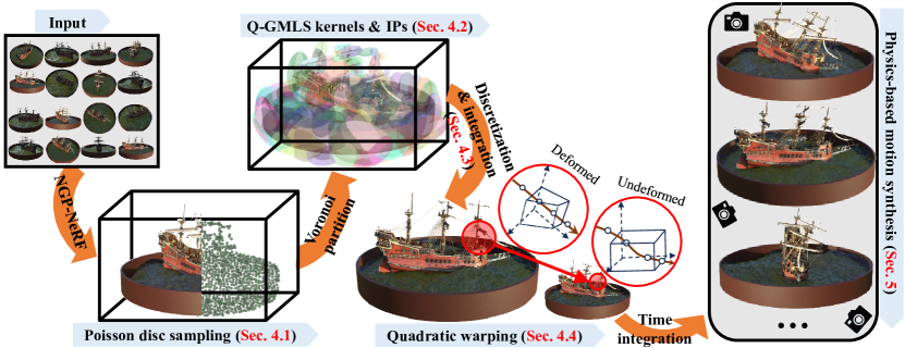
Figure 2: Pipeline overview: The input of PIE-NeRF is the same as other NeRF-based frameworks, which consists of a collection of images of a static scene. An adaptive Poisson disk sampling is followed to query the 3D geometry of the model, which are sparsified into $n$ Q-GMLS kernels. Integrator points are placed over the model, including centers of Q-GMLS kernels (i.e., kernel IPs). Discretization at kernels and numerical integration at IPs enable efficient synthesis of novel and physics-based elastodynamic motions. The quadratic warping scheme helps to better retrieve the color/texture of a deformed spatial position to render the final result.

3 Preliminary

To make the paper self-contained, we start with a brief review of some core techniques on which our pipeline is built. More details of our system are elaborated in § 4.

3.1 Neural radiance field

NeRF implicitly represents the geometry and appearance information of a 3D scene via a multi-layer perceptron (MLP) net. Given the camera parameters, a pixel’s color on the image plane is obtained via integrating the density and color along the ray. A spatial coordinate $\mathbf{p}$ and a ray direction $\mathbf{d}$ are often encoded as a feature vector $\psi_{\mathbf{p}},\psi_{\mathbf{d}}$ before being fed to the MLP for the prediction of density ($\sigma$) and color ($\mathbf{c}$). For instance, the vanilla NeRF [44] uses positional encoding to better tackle high-frequency information with MLPs. Our pipeline uses the instant neural graphics primitives (NGP) [50]. NGP adopts a multi-level hash-based encoding scheme and has demonstrated a strong performance in terms of both efficiency and quality.

3.2 Nonlinear elastodynamic

Following the classic Lagrangian mechanics [51], the dynamic equilibrium of a 3D model is characterized as:

$$\frac{\mathrm{d}}{\mathrm{d}t}\left(\frac{\partial L}{\partial\dot{\mathbf{q}}}\right)-\frac{\partial L}{\partial\mathbf{q}}=\mathbf{f}_{q},$$ (1)

where $L=T-U$ is Lagrangian i.e., the difference between the kinematic energy ($T$) and the potential energy ($U$) of the system. $\mathbf{q}$ and $\dot{\mathbf{q}}$ are generalized coordinate and velocity. $\mathbf{f}_{q}$ is the generalized external force. Given a time integration scheme such as implicit Euler: $\mathbf{q}_{n+1}=\mathbf{q}_{n}+h\dot{\mathbf{q}}_{n+1}$, $\dot{\mathbf{q}}_{n+1}=\dot{\mathbf{q}}_{n}+h\ddot{\mathbf{q}}_{n+1}$, Eq. (1) can be reformulated a set of nonlinear equations to be solved at each time step:

$$\mathbf{M}(\mathbf{q}_{n+1}-\mathbf{q}_{n}-h\dot{\mathbf{q}})=h^{2}\left(-\frac{\partial U}{\partial\mathbf{q}}+\mathbf{f}_{q}\right).$$ (2)

Here, the subscript indicates the time step index, and $h$ is the time step size. $\mathbf{q}_{n+1}$ is the unknown system coordinate to be solved, while all the kinematic variables of the previous time step such as $\mathbf{q}_{n}$ or $\dot{\mathbf{q}}_{n}$ are considered known. $-\partial U/\partial\mathbf{q}$ is the negative gradient of the potential, which embodies the internal force.

4 Our method

As shown in Fig. 2, the input of our system is a collection of images of a given 3D scene. We use NGP to encode positional and texture information and train the corresponding NeRF. Afterwards, we disperse particles into the scene. Those particles form an unstructured point-cloud-like proxy of the 3D model of interest. They are then grouped under a Voronoi partition, and the centers of Voronoi cells house the generalized coordinate of the system ($\mathbf{q}$ in Eq. (2)). We further assign multiple integrator points (IPs) to facilitate energy integration. A quadratic generalized moving least square (Q-GMLS) strategy is used to discretize the Lagrangian equation of Eq. (1). With the help of GPU, the simulation can be done at an interactive rate or even in real-time. We leverage the deformation information at IPs to infer the rest-pose position during NGP-based NeRF rendering. Thanks to NGP, this procedure is also in real-time. Our pipeline allows users to interact with a NeRF scene by applying external forces, position constraints etc., leading to novel and physics-grounded dynamic effects. Next, we give detailed expositions of each major step of the pipeline.

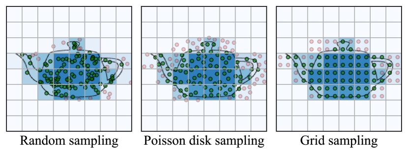
Figure 3: Particle sampling: Our method is compatible with most sampling algorithms – as long as particles cover the shape of the 3D model sufficiently well. In our implementation, we design a novel augmented Poisson disk sampling scheme that is fast and well captures the boundary of the model by default.

4.1 Augmented Poisson disk sampling

After the NGP-NeRF is trained, we choose a meshless way to model the geometry of the 3D shape. While the underlying goal of this step is similar to other static NeRF editing systems [85, 78, 57], being mesh-free makes our pipeline more flexible and versatile. In theory, any sampling method should work as long as the sampling particles sufficiently capture the boundary of the model. For instance, one can distribute particles by simply following the evenly-spaced grid (Fig. 3, right). Doing so is similar to using a grid-based cage to approximate the shape of the model [21].

Alternatively, we design an augmented Poisson disk sampling (PDS) strategy. The original PDS requires that the distance between any two particles be larger than a threshold $\bar{r}$. Starting from an initial point, PDS then tries to fill a banded ring between $\bar{r}$ and $2\bar{r}$ with new samples i.e., see [8]. Our observation is that more particles are needed at the boundary of the shape, which coincides with a sharp density variation. To this end, we adaptively adjust the sample radius $r$ based on the norm of the density gradient of NGP-NeRF $\|\nabla\sigma\|$ such that:

$$r=\max\left\{\bar{r},\kappa\frac{\bar{r}}{\sqrt{\|\nabla\sigma\|+\alpha}}\right\},$$ (3)

where $\alpha=10^{-3}$ is a small number avoiding the division-by-zero error. Eq. (3) suggests that the actual sample radius $r$ decreases when $\|\nabla\sigma\|$ is a large quantity. The density gradient $\|\nabla\sigma\|$ can be conveniently computed by differentiating the NPG-NeRF using AutoDiff [55]. We discard PDS particles whose density values are less than $\epsilon=10^{-2}$, which are visualized as pink dots in Fig. 3.

Our sampling ensures that the distance between a PDS particle at $\mathbf{x}$ and its nearest neighbor is at least $r(\mathbf{x})$, and we assign a volume of the PDS particle as:

$$V(\mathbf{x})=\frac{4}{3}\pi r^{3}(\mathbf{x}).$$ (4)

4.2 Q-GMLS kernels and integrator points

We perform a Voronoi partition [2] over PDS particles (see the inset) and use each Voronoi cell as a GMLS kernel for the body-wise displacement interpolation to reduce the computation overhead. Let $\Omega$ be the body of a 3D model in NeRF sampled by PDS particles with $n$ GMLS kernels. The classic MLS assumes a kernel possesses an affine displacement filed: $\mathbf{A}_{i}\mathbf{p}(\mathbf{x}_{i})$, where $\mathbf{x}_{i}$ is the center of the $i$-th kernel at the rest pose (green dots in the inset); $\mathbf{p}(\mathbf{x})=[1,\mathbf{x}^{\top}]^{\top}$. By minimizing a displacement-based target of: $\sum_{i=0}^{n}w(\mathbf{x}-\mathbf{x}_{i})\left\|\mathbf{A}\mathbf{p}(\mathbf{x}_{i})-\mathbf{u}_{i}\right\|^{2}$ one can obtain:

$$\mathbf{u}(\mathbf{x})=\sum_{i=1}^{n}\mathbf{u}_{i}N_{i}(\mathbf{x}).$$ (5)

Here $\mathbf{u}_{i}=\mathbf{u}(\mathbf{x}_{i})$ is the displacement of $i$-the kernel center; $N_{i}(\mathbf{x})=\mathbf{p}(\mathbf{x})^{\top}\mathbf{G}^{-1}(\mathbf{x})\mathbf{p}(\mathbf{x}_{i})w(\mathbf{x}-\mathbf{x_{i}})$, for $\mathbf{G}(\mathbf{x})=\sum_{i=1}^{n}w(\mathbf{x}-\mathbf{x}_{i})\mathbf{p}(\mathbf{x}_{i})\mathbf{p}(\mathbf{x}_{i})^{\top}$, is a shape-function-like trial function; and $w(\mathbf{d})=(1-\left\|\mathbf{d}\right\|^{2})^{3}$ is a MLS weighting function based on the distance between $\mathbf{x}$ and $\mathbf{x}_{i}$.

As the complexity of the simulation is up to $n$, we are in favor of using fewer kernels for faster computation. Doing so is likely to have $\mathbf{x}_{i}$ be colinear/coplanar, and $\mathbf{G}$ becomes singular. To improve the robustness of the kinematic interpolation of Eq. (5), GMLS takes the local deformation gradient information into account, which seeks the optimal $\mathbf{A}_{i}$ to minimize $\sum_{i=0}^{n}w(\mathbf{x}-\mathbf{x}_{i})\left\|\mathbf{A}_{i}\mathbf{p}(\mathbf{x}_{i})-\mathbf{u}_{i}\right\|^{2}+\sum_{i=0}^{n}\sum_{j=1}^{3}w(\mathbf{x}_{0}-\mathbf{x}_{i})\left\|\mathbf{A}_{i}\mathbf{p}_{,j}(\mathbf{x}_{i})-\mathbf{u}_{i,j}\right\|^{2}$. The comma here denotes the partial differentiation such that $\mathbf{u}_{i,1}=\partial\mathbf{u}_{i}/\partial x$, $\mathbf{u}_{i,2}=\partial\mathbf{u}_{i}/\partial y$, and $\mathbf{u}_{i,2}=\partial\mathbf{u}_{i}/\partial z$.

For thin and codimensional shapes, affine GMLS suffers from locking issues, wherein linearized shearing energy becomes orders stronger than nonlinear bending/twisting due to the interpolation error. This problem gets more serious with fewer kernels. To this end, we elevate the interpolation order, leading to quadratic GMLS or Q-GMLS, which assumes the per-kernel displacement field is quadratic. Namely, each $x$, $y$, or $z$ component of the displacement (i.e., for $j=1,2,3$ respectively) is fit by: $u_{ij}=\mathbf{x}_{i}^{\top}\mathbf{Q}^{j}_{i}\mathbf{x}_{i}+\mathbf{a}_{i}^{j\top}\mathbf{p}(\mathbf{x}_{i})$. Here $\mathbf{Q}_{i}^{j}$ is a symmetric tensor, and $\mathbf{a}_{i}^{j}\in\mathbb{R}^{4}$ is $j$-th row of $\mathbf{A}_{i}$. The Q-GMLS displacement interpolation can then be derived as:

$$\mathbf{u}(\mathbf{x})=\sum_{i=1}^{n}\big{[}\mathbf{u}_{i}N_{i}+\sum_{j}\mathbf{u}_{i,j}N_{i}^{j}+\sum_{j,k}\mathbf{u}_{i,jk}N_{i}^{jk}\big{]},$$ (6)

for $j,k=1,2,3$. Here

$$\begin{split}N_{i}(\mathbf{x})&=\mathbf{p}^{\top}(\mathbf{x})\mathbf{G}^{-1}(\mathbf{x})\mathbf{p}(\mathbf{x}_{i})w(\mathbf{x}-\mathbf{x}_{i}),\\ N_{i}^{j}(\mathbf{x})&=\mathbf{p}^{\top}(\mathbf{x})\mathbf{G}^{-1}(\mathbf{x})\mathbf{p}_{,j}(\mathbf{x}_{i})w(\mathbf{x}-\mathbf{x}_{i}),\\ N_{i}^{jk}(\mathbf{x})&=\mathbf{p}^{\top}(\mathbf{x})\mathbf{G}^{-1}(\mathbf{x})\mathbf{p}_{,jk}(\mathbf{x}_{i})w(\mathbf{x}-\mathbf{x}_{i})\end{split}$$ (7)

only depend on the rest-shape position $\mathbf{x}$, and

$$\mathbf{G}(\mathbf{x})=\sum_{i=1}^{n}w(\mathbf{x}-\mathbf{x}_{i})\left[\mathbf{p}(\mathbf{x}_{i})\mathbf{p}^{\top}(\mathbf{x}_{i})\right.\\ +\sum_{j}\mathbf{p}_{,j}(\mathbf{x}_{i})\mathbf{p}_{,j}^{\top}(\mathbf{x}_{i})+\sum_{j,k}\left.\mathbf{p}_{,jk}(\mathbf{x}_{i})\mathbf{p}^{\top}_{,jk}(\mathbf{x}_{i})\right].$$ (8)

It is convenient to re-organize Eq. (6) as:

$$\mathbf{u}(\mathbf{x})=\mathbf{J}(\mathbf{x})\mathbf{q},$$ (9)

such that $\mathbf{J}=[N_{1}\mathbf{I},N_{1}^{1}\mathbf{I},N_{1}^{2}\mathbf{I},...,N_{1}^{11}\mathbf{I},...]\in\mathbb{R}^{3\times 30n}$ and $\mathbf{q}=[\mathbf{u}_{1}^{\top},\mathbf{u}_{1,1}^{\top},\mathbf{u}_{1,2}^{\top},...,\mathbf{u}_{1,11}^{\top},...]^{\top}\in\mathbb{R}^{30n}$ are the Jacobi matrix and generalized coordinate (i.e., in Eq. (1)). Thus the generalized external force is computed via: $\mathbf{f}_{q}=\mathbf{J}^{\top}\mathbf{f}_{ext}$.

4.3 Energy integration

The total kinematic and potential energies of the model are:

$$T=\frac{1}{2}\int_{\Omega}\rho(\mathbf{x})\dot{\mathbf{x}}^{\top}\dot{\mathbf{x}}\mathrm{d}\Omega,\;\text{and}\;\;U=\int_{\Omega}\Psi(\mathbf{x})\mathrm{d}\Omega.$$ (10)

We want to avoid integrating over all the PDS particles. Therefore, our system includes another set of integrator points or IPs. Conceptually, IPs are similar to the quadrature points used in numerical integration [19], which allows us to substantially reduce the computational cost of full integrals in Eq. (10). In addition to the centers of Q-GMLS kernels i.e., kernel IPs, we add more IPs aiming to approximate Eq. (10) with high accuracy. Specifically, we initialize new IPs at the PDS particle which is the most distant from existing IPs to sample remote $T$ and $V$ values. This strategy however tends to favor PDS particles at the model’s boundary. As a result, we apply a few Lloyd relaxations [13] to new IPs while keeping kernel IPs fixed. The total number of IPs is bigger than the number of Q-GMLS kernels but they are of the same order, and we use $\mathcal{I}$ to denote the set of all the IPs.

4.4 Per-IP integration

We envision each IP as a small elastic cuboid $\Omega_{k}$ (see the inset) with three edges being $\mathbf{c}_{1}$, $\mathbf{c}_{2}$, $\mathbf{c}_{3}$ whose lengths are $h_{1}$, $h_{2}$, $h_{3}$ respectively. Its covariance matrix can be computed as: $\mathbf{C}=\sum_{j}V(\mathbf{x}_{j})\mathbf{x}_{j}\mathbf{x}_{j}^{\top}$, where the summation carries over K-nearest PDS particles whose rest positions are $\mathbf{x}_{j}$. Being a symmetric matrix, $\mathbf{C}$ always has three real non-negative eigen values namely, $\lambda_{1}$, $\lambda_{2}$, and $\lambda_{3}$. Note that coplanar geometry around an IP can make $\mathbf{C}$ singular. It is fine for numerical integration, suggesting the strains along certain directions are zero. We then set the ratio among $h_{i}$ to be the same as $\sqrt{\lambda_{i}}$ (i.e., $h_{1}:h_{2}:h_{3}$ equals $\sqrt{\lambda_{1}}:\sqrt{\lambda_{2}}:\sqrt{\lambda_{3}}$) while requiring $\Pi_{i}h_{i}=\sum_{j}V(\mathbf{x}_{j})$. Those two constraints allow us to compute $h_{1}$, $h_{2}$, and $h_{3}$ while $\mathbf{c}_{i}$ are the corresponding eigen vectors.

The total kinematic energy can now be approximated as:

$$T=\frac{1}{2}\int_{\Omega}\rho(\mathbf{x})\dot{\mathbf{x}}^{\top}\dot{\mathbf{x}}\mathrm{d}\Omega=\frac{1}{2}\dot{\mathbf{q}}^{\top}\left(\int_{\Omega}\rho\mathbf{J}^{\top}\mathbf{J}\mathrm{d}\Omega\right)\dot{\mathbf{q}}\\ \approx\frac{1}{2}\dot{\mathbf{q}}^{\top}\left[\sum_{\mathbf{x}_{k}\in\mathcal{I}}\rho V_{k}\mathbf{J}^{\top}(\mathbf{x}_{k})\mathbf{J}(\mathbf{x}_{k})\right]\dot{\mathbf{q}},$$ (11)

and $\mathbf{M}=\sum_{\mathbf{x}_{k}\in\mathcal{I}}\rho V_{k}\mathbf{J}^{\top}(\mathbf{x}_{k})\mathbf{J}(\mathbf{x}_{k})$ is the mass matrix. Note that $V_{k}=h_{1}h_{2}h_{3}$ is the estimated volume of the IP cuboid, not the volume of the PDS particle. $\rho$ is the density of the 3D model, which should not be confused with $\sigma$.

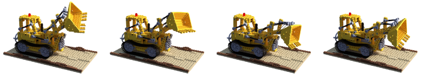
Figure 4: Elastically deforming excavator: The excavator is a standard benchmark for NeRF-based frameworks. We use this classic model to showcase the capability of PIE-NeRF, which generates interesting and novel dynamic effects in real time.

Integrating the potential energy $U$ is handled in a similar way. Under the assumption of hyperelasticity, the energy density $\Psi(\mathbf{x})$ depends on the deformation gradient at $\mathbf{x}$: $\mathbf{F}=\nabla\mathbf{\mathbf{u}(\mathbf{x})+\mathbf{I}}\in\mathbb{R}^{3\times 3}$. According to Eq. (9), the deformation gradient at the $k$-th IP is:

$$\mathbf{F}(\mathbf{x}_{k})=\mathbf{F}_{k}=\mathbf{q}\cdot\nabla\mathbf{J}^{\top}(\mathbf{x}_{k})+\mathbf{I}=\mathbf{q}\cdot\nabla\mathbf{J}^{\top}_{k}+\mathbf{I}.$$ (12)

$\mathbf{J}_{k}\in\mathbb{R}^{3\times 30n}$ is the Jacobi corresponding to the IP, and $\nabla\mathbf{J}^{\top}_{k}\in\mathbb{R}^{30n\times 3\times 3}$ is a third tensor. The potential accumulated at the IP is estimated by integrating over its cuboid ($\Omega_{k}$) assuming the IP lies at the center:

$$U_{k}=\int_{\Omega_{k}}\Psi(\mathbf{F}(\mathbf{h}))=\int_{-\frac{h_{1}}{2}}^{\frac{h_{1}}{2}}\int_{-\frac{h_{2}}{2}}^{\frac{h_{2}}{2}}\int_{-\frac{h_{3}}{2}}^{\frac{h_{3}}{2}}\Psi(\mathbf{F}(\mathbf{h})).$$ (13)

Here, $\mathbf{h}$ is the local coordinate spanning $\Omega_{k}$, and $\mathbf{x}_{k}$ aligns with $\mathbf{h}=0$. When $\mathbf{h}\neq 0$, we first-order approximate $\mathbf{F}$ as:

$$\mathbf{F}(\mathbf{h})\approx\mathbf{F}(0)+\nabla\mathbf{F}(0)\cdot\mathbf{h}=\mathbf{F}(\mathbf{x}_{k})+\nabla\mathbf{F}(\mathbf{x}_{k})\cdot\mathbf{h}.$$ (14)

This makes sense because Q-GMLS assumes $\mathbf{u}$ is quadratic, which has a linearly-vary deformation gradient. Therefore, the approximate in Eq. (14) should be exact. $\nabla\mathbf{F}$ can be computed by differentiating Eq. (12):

$$\nabla\mathbf{F}(\mathbf{x}_{k})=\mathbf{q}\cdot\nabla^{2}\mathbf{J}^{\top}_{k}=\mathbf{H}_{k}\cdot\mathbf{q}.$$ (15)

Here $\mathbf{H}=\partial\nabla\mathbf{J}^{\top}/\partial\mathbf{x}$ is a fourth tensor. This computation boils down to evaluating first- and second-derivatives of $N_{i}$, $N_{i}^{j}$, and $N_{i}^{jk}$, and can be pre-computed per Eq. (7).

Given an elastic material model $\Psi(\mathbf{F})$, the total potential can then be computed via:

$$U\approx\sum_{\mathbf{x}_{k}\in\mathcal{I}}\int_{\Omega_{k}}\Psi\left(\mathbf{F}(0)+\mathbf{H}_{k}:(\mathbf{q}\mathbf{h}^{\top})\right)\mathrm{d}\Omega_{k}.$$ (16)

The actual integration computation relies on the specific formulation of $\Psi(\mathbf{F})$. Please refer to the supplementary document for detailed derivations of some commonly-used material models such as ARAP and Neo-Hookean.

4.5 System assembly and solve

With energy integrals, we can assemble Eq. (2). The generalized internal force is $\mathbf{f}_{int}=-\partial U/\partial\mathbf{q}$, and it can be conveniently computed by the chain rule:

$$\mathbf{f}_{int}=-\frac{\partial\Psi}{\partial\mathbf{F}}:\frac{\partial\mathbf{F}}{\partial\mathbf{q}}=-\mathbf{P}:\nabla\mathbf{J},$$ (17)

where $\mathbf{P}$ is the first Piola-Kirchhoff stress. This is a $30n$-dimension dense system as all Q-GMLS kernels have global influences. We use Newton’s method to solve this system iteratively. Each Newton iteration solves a linearized problem for an incremental improvement $\Delta\mathbf{q}$:

$$\left(\mathbf{M}+h^{2}\frac{\partial\mathbf{f}_{int}}{\partial\mathbf{q}}\right)\Delta\mathbf{q}=\mathbf{M}(\mathbf{q}_{n}+h\dot{\mathbf{q}}_{n})+h^{2}\mathbf{J}^{\top}\mathbf{f}_{ext},$$ (18)

where $\partial\mathbf{f}_{int}/\partial\mathbf{q}$ is the second differentiation of the total potential $U$ known as the tangent stiffness matrix. $\mathbf{f}_{ext}$ is the external forces applied to the model. It is projected to the Q-GMLS kinematic space by left multiplying $\mathbf{J}^{\top}$.

4.6 NeRF rendering using quadratic warping

After the deformed model geometry is computed, we leverage the NGP-NeRF that is built for its rest shape to synthesize both novel views and novel deformations. Whenever we query the NGP-NeRF for a deformed location $\tilde{\mathbf{x}}$ along a ray, we warp this position to its rest configuration $\mathbf{x}$, ideally through $\mathbf{x}=\tilde{\mathbf{x}}-\mathbf{u}(\mathbf{x})$. Unfortunately as $\mathbf{x}$ is unknown here, we cannot obtain $\mathbf{u}(\mathbf{x})$ directly with Eq. (9). Instead, we approximate $\mathbf{u}(\mathbf{x})$ based on the displacements at nearby (deformed) IPs. The general rationale is that if $\tilde{\mathbf{x}}$ is sufficiently close to an IP, we can Taylor expand the IP’s displacement to estimate $\mathbf{u}(\mathbf{x})$. As IPs are sparse, it is possible that $\tilde{\mathbf{x}}$ is not particularly close to one IP. In this case, we find three nearest IPs and average Taylor expansions at those IPs based on the inverse distance weight.

For the IP at $\mathbf{x}_{k}$, we have:

$$\tilde{\mathbf{x}}-\tilde{\mathbf{x}}_{k}=\mathbf{u}(\mathbf{x})-\mathbf{u}(\mathbf{x}_{k})\approx\nabla\mathbf{u}(\mathbf{x}_{k})(\mathbf{x}_{k}-\mathbf{x})\\ +\frac{1}{2}\left(\nabla\mathbf{F}(\mathbf{x}_{k})\cdot(\mathbf{x}_{k}-\mathbf{x})\right)\cdot(\mathbf{x}_{k}-\mathbf{x}).$$ (19)

We can then compute $\mathbf{x}$ via solving a nonlinear system of:

$$\mathbf{A}(\mathbf{x})\mathbf{x}=\mathbf{b},$$ (20)

where

$$\begin{array}[]{l}\displaystyle\mathbf{A}(\mathbf{x})=\frac{1}{2}\nabla\mathbf{F}(\mathbf{x}_{k})\cdot\mathbf{x}_{k}+\nabla\mathbf{F}(\mathbf{x}_{k})\cdot\mathbf{x},\\ \displaystyle\mathbf{b}=\tilde{\mathbf{x}}-\tilde{\mathbf{x}}_{k}-\frac{1}{2}\nabla\mathbf{F}(\mathbf{x}_{k}):\left(\mathbf{x}_{k}\mathbf{x}^{\top}_{k}\right).\end{array}$$ (21)

While the analytic solution of Eq. (20) can be derived, we find Newton’s method starting from the guess of $\mathbf{x}=\mathbf{x}_{k}$ is effective. The system converges within tens of iterations, and each iteration only solves a 3 by 3 linear system.

This strategy of quadratic warping fully exploits the prior of $\mathbf{u}$ being the quadratic displacement field. If we only use the first-order Taylor expansion to estimate the undeformed position of $\tilde{\mathbf{x}}$, as chosen in most existing NeRF editing systems [57, 78], visual artifacts can be observed under large deformations (see Fig. 8).

5 Experiments

We implemented PIE-NeRF pipeline using Python and C++. The simulation module was based on CUDA. In addition, we used PyTorch [26] and Taichi [24] to implement a modified instant-NGP [50] for ray warping (§ 4.6). Our hardware platform is a desktop computer equipped with an Intel i7-12700F CPU and an NVIDIA 3090 GPU.

Datasets We evaluate PIE-NeRF with several NeRF scenes. In addition to original NeRF datasets, we utilize BlenderNeRF [60] to synthesize additional scenes including codimensional objects. We used 100 multi-view images for each scene as inputs for our NGP-NeRF training.

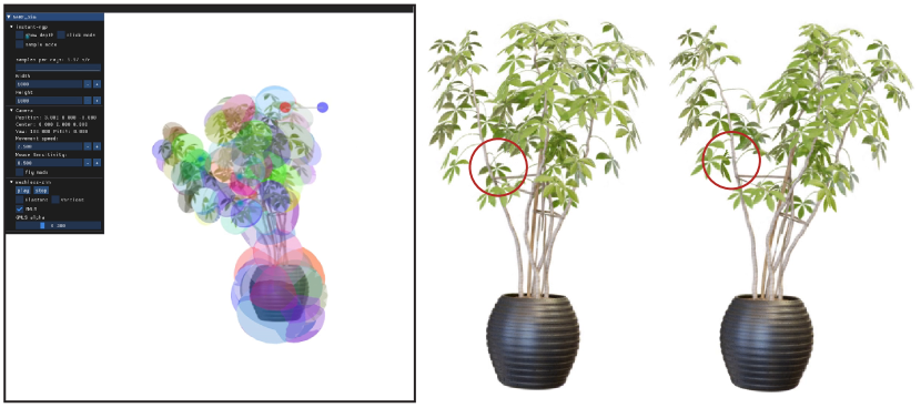
Figure 5: Interactive NeRF deformation: We developed an intuitive UI for users to interact with NeRF scenes like applying external forces and position constraints. Q-GMLS kernels can also be set adaptively to capture local dynamics as highlighted.

5.1 Interactive and dynamic NeRF simulation

PIE-NeRF formulates nonlinear dynamics of NeRF models with the generalized coordinate and Lagrangian equations (i.e., Eq. (1)), which makes the computation independent of the PDS sampling resolution. We find that a few dozen Q-GMLS kernels are often sufficient to model complex models. The corresponding computation is light-weight and can be processed in real-time on the GPU (see Fig. 4). Therefore, interactive physics-based manipulation of the NeRF scene becomes possible. To this end, we also implemented a user-friendly interface as shown in Fig. 5, left. With the interface, users can intuitively apply external forces to the model, and observe the resulting novel motions interactively. The users have full control over the trade-off between visual richness and the efficiency of the simulation. For instance, one can create a dedicated kernel to capture local dynamics at specific foliage of the plant (Fig. 5, right).

Figure 6: Volume preservation test: PIE-NeRF is capable of incorporating any real-world material models. In this example, we apply a position constraint to compress a chocolate jelly. ARAP energy, widely used in exiting NeRF editing systems [84], collapses unnaturally. With Neo-Hookean energy, PIE-NeRF can better synthesize this procedure.

5.2 Physics-grounded pose synthesis

Being a physics-based framework, PIE-NeRF is able to model any nonlinear hyperelastic materials to match real-world observations. This enhances existing NeRF editing systems, which are mostly based on geometry-based heuristic energy models like ARAP. Fig. 6 reports a comparison using the Neo-Hookean material [bonet1997nonlinear] and ARAP to compress chocolate jelly with NeRF. The energy density of Neo-Hookean material is:

$$\Psi=\frac{\mu}{2}\left(I_{C}-3\right)-\mu\log J+\frac{\lambda}{2}\log^{2}J,$$ (22)

where $\mu$, $\lambda$ are material parameters (a.k.a Lamé coefficients); $I_{C}=\text{tr}(\mathbf{F}^{\top}\mathbf{F})$; and $J=\text{det}(\mathbf{F})$. The log barrier $\log J$ in Neo-Hookean energy strongly preserves the volume of the object. This feature is clearly demonstrated in Fig. 6. As the compression rate increases, ARAP jelly (on the top) loses nearly $40\%$ of the original volume (visualized as bar graphs at the bottom in Fig. 6).

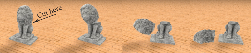
Figure 7: Topology change and shadows: We edit kernel weights to cut the sculpture, which then falls on the floor. We then compute the depth map from NGP-NeRF and generate the moving shadow using shadow maps.

Handle topology change.  Being meshless makes PIE-NeRF less sensitive to topology changes. As shown in Fig. 7, we cut the NeRF sculpture by modifying Q-GMLS weight functions. Besides that, there is no need for extra safeguards for dealing with the change of the mesh connectivity and resolution at the cutting area. In this example, we extract the depth image with NGP-NeRF, from which a shadow map can be generated for shadow synthesis.

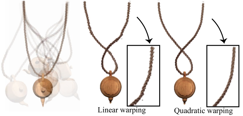
Figure 8: Codimensional rod and quadratic warping: Q-GMLS uses quadratic “shape functions” which better handle thin geometries as shown in this example. The rod undergoes large bending and twisting deformation. Linear ray warping tends to generate artifacts, while the quadratic warping used in PIE-NeRF accurately fetches the color information and produces more plausible results.

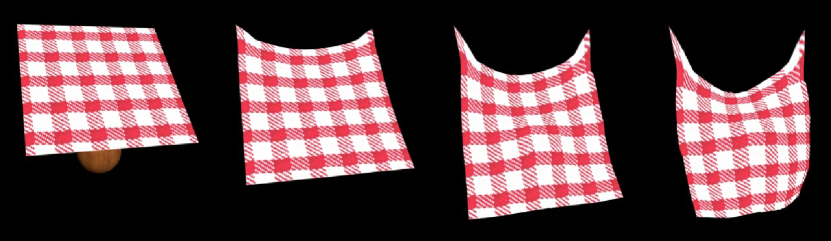
Figure 9: Thin shell simulation: PIE-NeRF is also compatible with thin shells. The NeRF-based cloth drops under gravity and hits a sphere.

Codimensional shapes. Q-GMLS can capture nonlinear dynamics of thin shapes without locking artifacts. To show this feature, we report two experiments of models with codimensional geometries. Fig. 8 gives snapshots of simulating an elastic rod attached to a teapot. Linear MLS [49] could yield shearing locking easily, while quadratic interpolation avoids this issue. The incorporation of deformation gradient during the shape function computation (i.e., Eq (7)) makes our discretization robust, and the corresponding quadratic warping method yields better images than naïve linear warping as shown in the right of the figure. Fig. 9 shows another example where a thin-shell cloth, implicitly encoded with NGP-NeRF, collides with a sphere. One will easily observe locking issues if linear MLS is used. Please refer to supplementary documents for more results.

Comparison with PAC-NeRF. PAC-NeRF [35] is a recent contribution also aiming to combine physical models with NeRF-based representations. The underlying numerical solver, on the other hand, is based on the material point method (MPM) [6]. While MPM excels in handling complicated, multi-phase physics, it does not synergize well with NeRF-based rendering. Specifically, under large deformation, PAC-NeRF fails to map material points back to their rest-pose positions accurately due to excessive g2p2g smoothing, which leads to over-blurred results at local fine shapes. We show a side-by-side comparison in Fig. 11.

5.3 Time performance

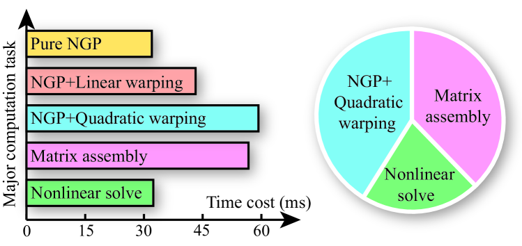
Figure 10: Time breakdown: During the simulation, there are three major steps for PIE-NeRF, namely matrix assembly, solve, and warping. Thanks to Q-GMLS-based reduction, they are all manageable making the simulation interactive. The percentage of each step is visualized as a pie diagram on the right.

Fig. 10 reports a breakdown of the run time performance of our PIE-NeRF pipeline for Fig. 5. Three major tasks for the simulation at the runtime are matrix assembly, nonlinear solve, and quadratic warping. The matrix assembly requires an integral over all the IPs, leading to a dense $30n$ by $30n$ system. We use Cholesky factorization to solve the resulting Newton system (Eq. (18)). In general, a couple of iterations will converge the system so that we forward to the next time step. As shown in the figure, quadratic warping used in PIE-NeRF is slightly more expensive than linear warping. However, those extra costs return much improved visual results (Fig. 8) in general. The percentages of each step are shown in the pie diagram.

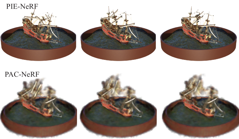
Figure 11: PIE vs PAC: PAC-NeRF [35] is a closely relevant competitor. A major limitation of PAC-NeRF is the rendering. It is less intuitive to infer the right color/texture information under large deformation using MPM. PIE-NeRF overcomes this limitation with ease. Using implicit time integration, PIE-NeRF runs much faster than PAC-NeRF (two orders in this example).

6 Conclusion

PIE-NeRF is a physics-NeRF simulation pipeline. It is directly based on PDS particles sampled over the NeRF scene and applies a Q-GMLS model reduction to lower the computational overhead of the simulation. As a result, PIE-NeRF faithfully characterizes various real-world material models. Its meshless representation makes the simulation flexible, and topology change can be well accommodated. The quadratic interpolation scheme is not only helpful in tackling thin-geometry models but also leads to better image synthesis with NGP-NeRF. We hope PIE-NeRF contributes new ingredients to the existing NeRF ecosystem. Based on PIE-NerF, it is possible to integrate more (better and faster) simulation and graphics techniques to deep 3D vision applications to imbue vivid, realistic, real-time physics into static or dynamic environments. Along this exciting endeavor, we will also explore other opportunities, such as Gaussian splatting-based techniques [31], and ultimately reach what you see is what you simulate, WS².

References

- [1] Carla Antoci, Mario Gallati, and Stefano Sibilla. Numerical simulation of fluid–structure interaction by sph. Computers & structures, 85(11-14):879–890, 2007.
- [2] Franz Aurenhammer. Voronoi diagrams—a survey of a fundamental geometric data structure. ACM Computing Surveys (CSUR), 23(3):345–405, 1991.
- [3] Chong Bao, Yinda Zhang, Bangbang Yang, Tianxing Fan, Zesong Yang, Hujun Bao, Guofeng Zhang, and Zhaopeng Cui. Sine: Semantic-driven image-based nerf editing with prior-guided editing field. In Proceedings of the IEEE/CVF Conference on Computer Vision and Pattern Recognition, pages 20919–20929, 2023.
- [4] D BARAFF. Large steps in cloth simulation. In SIGGRAPH’98 Proceedings, pages 43–54, 1998.
- [5] Jernej Barbič and Doug L James. Real-time subspace integration for st. venant-kirchhoff deformable models. ACM transactions on graphics (TOG), 24(3):982–990, 2005.
- [6] S. Bardenhagen and Edward Kober. The generalized interpolation material point method. CMES - Computer Modeling in Engineering and Sciences, 5, 06 2004.
- [7] Ted Belytschko, Yury Krongauz, Daniel Organ, Mark Fleming, and Petr Krysl. Meshless methods: an overview and recent developments. Computer methods in applied mechanics and engineering, 139(1-4):3–47, 1996.
- [8] Robert Bridson. Fast poisson disk sampling in arbitrary dimensions. In ACM SIGGRAPH 2007 Sketches, SIGGRAPH ’07, page 22–es, New York, NY, USA, 2007. Association for Computing Machinery.
- [9] Morten Bro-Nielsen and Stephane Cotin. Real-time volumetric deformable models for surgery simulation using finite elements and condensation. In Computer graphics forum, volume 15, pages 57–66. Wiley Online Library, 1996.
- [10] Ang Cao and Justin Johnson. Hexplane: A fast representation for dynamic scenes. In Proceedings of the IEEE/CVF Conference on Computer Vision and Pattern Recognition, pages 130–141, 2023.
- [11] Jun-Kun Chen, Jipeng Lyu, and Yu-Xiong Wang. Neuraleditor: Editing neural radiance fields via manipulating point clouds. In Proceedings of the IEEE/CVF Conference on Computer Vision and Pattern Recognition, pages 12439–12448, 2023.
- [12] Jiahua Dong and Yu-Xiong Wang. Vica-nerf: View-consistency-aware 3d editing of neural radiance fields. In Thirty-seventh Conference on Neural Information Processing Systems, 2023.
- [13] Qiang Du, Maria Emelianenko, and Lili Ju. Convergence of the lloyd algorithm for computing centroidal voronoi tessellations. SIAM journal on numerical analysis, 44(1):102–119, 2006.
- [14] Yilun Du, Yinan Zhang, Hong-Xing Yu, Joshua B Tenenbaum, and Jiajun Wu. Neural radiance flow for 4d view synthesis and video processing. In 2021 IEEE/CVF International Conference on Computer Vision (ICCV), pages 14304–14314. IEEE Computer Society, 2021.
- [15] Thomas-Peter Fries, Hermann G Matthies, et al. Classification and overview of meshfree methods. Department of Mathematics and Computer Science, Technical University of Braunschweig, 2003.
- [16] Chen Gao, Ayush Saraf, Johannes Kopf, and Jia-Bin Huang. Dynamic view synthesis from dynamic monocular video. In Proceedings of the IEEE/CVF International Conference on Computer Vision, pages 5712–5721, 2021.
- [17] Stephan J Garbin, Marek Kowalski, Virginia Estellers, Stanislaw Szymanowicz, Shideh Rezaeifar, Jingjing Shen, Matthew Johnson, and Julien Valentin. Voltemorph: Realtime, controllable and generalisable animation of volumetric representations. arXiv preprint arXiv:2208.00949, 2022.
- [18] Stephan J Garbin, Marek Kowalski, Matthew Johnson, Jamie Shotton, and Julien Valentin. Fastnerf: High-fidelity neural rendering at 200fps. In Proceedings of the IEEE/CVF International Conference on Computer Vision, pages 14346–14355, 2021.
- [19] Thomas Gerstner and Michael Griebel. Numerical integration using sparse grids. Numerical algorithms, 18(3-4):209–232, 1998.
- [20] Bingchen Gong, Yuehao Wang, Xiaoguang Han, and Qi Dou. Recolornerf: Layer decomposed radiance field for efficient color editing of 3d scenes. arXiv preprint arXiv:2301.07958, 2023.
- [21] Xiang Guo, Guanying Chen, Yuchao Dai, Xiaoqing Ye, Jiadai Sun, Xiao Tan, and Errui Ding. Neural deformable voxel grid for fast optimization of dynamic view synthesis. In Proceedings of the Asian Conference on Computer Vision, pages 3757–3775, 2022.
- [22] Xiang Guo, Jiadai Sun, Yuchao Dai, Guanying Chen, Xiaoqing Ye, Xiao Tan, Errui Ding, Yumeng Zhang, and Jingdong Wang. Forward flow for novel view synthesis of dynamic scenes. In Proceedings of the IEEE/CVF International Conference on Computer Vision, pages 16022–16033, 2023.
- [23] Ayaan Haque, Matthew Tancik, Alexei A Efros, Aleksander Holynski, and Angjoo Kanazawa. Instruct-nerf2nerf: Editing 3d scenes with instructions. arXiv preprint arXiv:2303.12789, 2023.
- [24] Yuanming Hu, Tzu-Mao Li, Luke Anderson, Jonathan Ragan-Kelley, and Frédo Durand. Taichi: a language for high-performance computation on spatially sparse data structures. ACM Transactions on Graphics (TOG), 38(6):1–16, 2019.
- [25] Sungwon Hwang, Junha Hyung, Daejin Kim, Min-Jung Kim, and Jaegul Choo. Faceclipnerf: Text-driven 3d face manipulation using deformable neural radiance fields. In Proceedings of the IEEE/CVF International Conference on Computer Vision, pages 3469–3479, 2023.
- [26] Sagar Imambi, Kolla Bhanu Prakash, and GR Kanagachidambaresan. Pytorch. Programming with TensorFlow: Solution for Edge Computing Applications, pages 87–104, 2021.
- [27] Ajay Jain, Matthew Tancik, and Pieter Abbeel. Putting nerf on a diet: Semantically consistent few-shot view synthesis. In Proceedings of the IEEE/CVF International Conference on Computer Vision, pages 5885–5894, 2021.
- [28] Clément Jambon, Bernhard Kerbl, Georgios Kopanas, Stavros Diolatzis, George Drettakis, and Thomas Leimkühler. Nerfshop: Interactive editing of neural radiance fields. Proceedings of the ACM on Computer Graphics and Interactive Techniques, 6(1), 2023.
- [29] Kaiwen Jiang, Shu-Yu Chen, Feng-Lin Liu, Hongbo Fu, and Lin Gao. Nerffaceediting: Disentangled face editing in neural radiance fields. In SIGGRAPH Asia 2022 Conference Papers, pages 1–9, 2022.
- [30] Kacper Kania, Kwang Moo Yi, Marek Kowalski, Tomasz Trzciński, and Andrea Tagliasacchi. Conerf: Controllable neural radiance fields. In Proceedings of the IEEE/CVF Conference on Computer Vision and Pattern Recognition, pages 18623–18632, 2022.
- [31] Bernhard Kerbl, Georgios Kopanas, Thomas Leimkühler, and George Drettakis. 3d gaussian splatting for real-time radiance field rendering. ACM Transactions on Graphics (ToG), 42(4):1–14, 2023.
- [32] Theodore Kim and David Eberle. Dynamic deformables: implementation and production practicalities (now with code!). In ACM SIGGRAPH 2022 Courses, pages 1–259. 2022.
- [33] Sosuke Kobayashi, Eiichi Matsumoto, and Vincent Sitzmann. Decomposing nerf for editing via feature field distillation. Advances in Neural Information Processing Systems, 35:23311–23330, 2022.
- [34] Verica Lazova, Vladimir Guzov, Kyle Olszewski, Sergey Tulyakov, and Gerard Pons-Moll. Control-nerf: Editable feature volumes for scene rendering and manipulation. In Proceedings of the IEEE/CVF Winter Conference on Applications of Computer Vision, pages 4340–4350, 2023.
- [35] Xuan Li, Yi-Ling Qiao, Peter Yichen Chen, Krishna Murthy Jatavallabhula, Ming Lin, Chenfanfu Jiang, and Chuang Gan. Pac-nerf: Physics augmented continuum neural radiance fields for geometry-agnostic system identification. arXiv preprint arXiv:2303.05512, 2023.
- [36] Zhengqi Li, Simon Niklaus, Noah Snavely, and Oliver Wang. Neural scene flow fields for space-time view synthesis of dynamic scenes. In Proceedings of the IEEE/CVF Conference on Computer Vision and Pattern Recognition, pages 6498–6508, 2021.
- [37] Gui-Rong Liu and D Karamanlidis. Mesh free methods: moving beyond the finite element method. Appl. Mech. Rev., 56(2):B17–B18, 2003.
- [38] Jia-Wei Liu, Yan-Pei Cao, Weijia Mao, Wenqiao Zhang, David Junhao Zhang, Jussi Keppo, Ying Shan, Xiaohu Qie, and Mike Zheng Shou. Devrf: Fast deformable voxel radiance fields for dynamic scenes. Advances in Neural Information Processing Systems, 35:36762–36775, 2022.
- [39] Lingjie Liu, Jiatao Gu, Kyaw Zaw Lin, Tat-Seng Chua, and Christian Theobalt. Neural sparse voxel fields. Advances in Neural Information Processing Systems, 33:15651–15663, 2020.
- [40] Ruiyang Liu, Jinxu Xiang, Bowen Zhao, Ran Zhang, Jingyi Yu, and Changxi Zheng. Neural impostor: Editing neural radiance fields with explicit shape manipulation. arXiv preprint arXiv:2310.05391, 2023.
- [41] Steven Liu, Xiuming Zhang, Zhoutong Zhang, Richard Zhang, Jun-Yan Zhu, and Bryan Russell. Editing conditional radiance fields. In Proceedings of the IEEE/CVF international conference on computer vision, pages 5773–5783, 2021.
- [42] Sebastian Martin, Peter Kaufmann, Mario Botsch, Eitan Grinspun, and Markus Gross. Unified simulation of elastic rods, shells, and solids. ACM Transactions on Graphics (TOG), 29(4):1–10, 2010.
- [43] Aryan Mikaeili, Or Perel, Mehdi Safaee, Daniel Cohen-Or, and Ali Mahdavi-Amiri. Sked: Sketch-guided text-based 3d editing. In Proceedings of the IEEE/CVF International Conference on Computer Vision, pages 14607–14619, 2023.
- [44] Ben Mildenhall, Pratul P. Srinivasan, Matthew Tancik, Jonathan T. Barron, Ravi Ramamoorthi, and Ren Ng. NeRF: Representing scenes as neural radiance fields for view synthesis. In The European Conference on Computer Vision (ECCV), 2020.
- [45] Matthias Müller and Nuttapong Chentanez. Solid simulation with oriented particles. In ACM SIGGRAPH 2011 papers, pages 1–10. 2011.
- [46] Matthias Müller and Markus H Gross. Interactive virtual materials. In Graphics interface, volume 2004, pages 239–246, 2004.
- [47] Matthias Müller, Bruno Heidelberger, Marcus Hennix, and John Ratcliff. Position based dynamics. Journal of Visual Communication and Image Representation, 18(2):109–118, 2007.
- [48] Matthias Müller, Bruno Heidelberger, Matthias Teschner, and Markus Gross. Meshless deformations based on shape matching. ACM transactions on graphics (TOG), 24(3):471–478, 2005.
- [49] Matthias Müller, Richard Keiser, Andrew Nealen, Mark Pauly, Markus Gross, and Marc Alexa. Point based animation of elastic, plastic and melting objects. In Proceedings of the 2004 ACM SIGGRAPH/Eurographics symposium on Computer animation, pages 141–151, 2004.
- [50] Thomas Müller, Alex Evans, Christoph Schied, and Alexander Keller. Instant neural graphics primitives with a multiresolution hash encoding. ACM Trans. Graph., 41(4), jul 2022.
- [51] Richard M Murray. Nonlinear control of mechanical systems: A lagrangian perspective. Annual Reviews in Control, 21:31–42, 1997.
- [52] Andrew Nealen, Matthias Müller, Richard Keiser, Eddy Boxerman, and Mark Carlson. Physically based deformable models in computer graphics. In Computer graphics forum, volume 25, pages 809–836. Wiley Online Library, 2006.
- [53] Keunhong Park, Utkarsh Sinha, Jonathan T Barron, Sofien Bouaziz, Dan B Goldman, Steven M Seitz, and Ricardo Martin-Brualla. Nerfies: Deformable neural radiance fields. In Proceedings of the IEEE/CVF International Conference on Computer Vision, pages 5865–5874, 2021.
- [54] Keunhong Park, Utkarsh Sinha, Peter Hedman, Jonathan T Barron, Sofien Bouaziz, Dan B Goldman, Ricardo Martin-Brualla, and Steven M Seitz. Hypernerf: A higher-dimensional representation for topologically varying neural radiance fields. arXiv preprint arXiv:2106.13228, 2021.
- [55] Adam Paszke, Sam Gross, Soumith Chintala, Gregory Chanan, Edward Yang, Zachary DeVito, Zeming Lin, Alban Desmaison, Luca Antiga, and Adam Lerer. Automatic differentiation in pytorch. 2017.
- [56] Mark Pauly, Richard Keiser, Leif P Kobbelt, and Markus Gross. Shape modeling with point-sampled geometry. ACM Transactions on Graphics (TOG), 22(3):641–650, 2003.
- [57] Yicong Peng, Yichao Yan, Shengqi Liu, Yuhao Cheng, Shanyan Guan, Bowen Pan, Guangtao Zhai, and Xiaokang Yang. Cagenerf: Cage-based neural radiance field for generalized 3d deformation and animation. Advances in Neural Information Processing Systems, 35:31402–31415, 2022.
- [58] Sergey Prokudin, Qianli Ma, Maxime Raafat, Julien Valentin, and Siyu Tang. Dynamic point fields. arXiv preprint arXiv:2304.02626, 2023.
- [59] Albert Pumarola, Enric Corona, Gerard Pons-Moll, and Francesc Moreno-Noguer. D-nerf: Neural radiance fields for dynamic scenes. In Proceedings of the IEEE/CVF Conference on Computer Vision and Pattern Recognition, pages 10318–10327, 2021.
- [60] Maxime Raafat. BlenderNeRF, May 2023.
- [61] Viktor Rudnev, Mohamed Elgharib, William Smith, Lingjie Liu, Vladislav Golyanik, and Christian Theobalt. Nerf for outdoor scene relighting. In European Conference on Computer Vision, pages 615–631. Springer, 2022.
- [62] Eftychios Sifakis and Jernej Barbic. Fem simulation of 3d deformable solids: a practitioner’s guide to theory, discretization and model reduction. In Acm siggraph 2012 courses, pages 1–50. 2012.
- [63] Hyeonseop Song, Seokhun Choi, Hoseok Do, Chul Lee, and Taehyeong Kim. Blending-nerf: Text-driven localized editing in neural radiance fields. In Proceedings of the IEEE/CVF International Conference on Computer Vision, pages 14383–14393, 2023.
- [64] Olga Sorkine and Marc Alexa. As-rigid-as-possible surface modeling. In Symposium on Geometry processing, volume 4, pages 109–116. Citeseer, 2007.
- [65] Pratul P Srinivasan, Boyang Deng, Xiuming Zhang, Matthew Tancik, Ben Mildenhall, and Jonathan T Barron. Nerv: Neural reflectance and visibility fields for relighting and view synthesis. In Proceedings of the IEEE/CVF Conference on Computer Vision and Pattern Recognition, pages 7495–7504, 2021.
- [66] Denis Steinemann, Miguel A Otaduy, and Markus Gross. Fast adaptive shape matching deformations. In Proceedings of the 2008 ACM SIGGRAPH/eurographics symposium on computer animation, pages 87–94, 2008.
- [67] Jingxiang Sun, Xuan Wang, Yong Zhang, Xiaoyu Li, Qi Zhang, Yebin Liu, and Jue Wang. Fenerf: Face editing in neural radiance fields. In Proceedings of the IEEE/CVF Conference on Computer Vision and Pattern Recognition, pages 7672–7682, 2022.
- [68] Demetri Terzopoulos, John Platt, Alan Barr, and Kurt Fleischer. Elastically deformable models. In Proceedings of the 14th annual conference on Computer graphics and interactive techniques, pages 205–214, 1987.
- [69] Edgar Tretschk, Ayush Tewari, Vladislav Golyanik, Michael Zollhöfer, Christoph Lassner, and Christian Theobalt. Non-rigid neural radiance fields: Reconstruction and novel view synthesis of a dynamic scene from monocular video. In Proceedings of the IEEE/CVF International Conference on Computer Vision, pages 12959–12970, 2021.
- [70] Can Wang, Menglei Chai, Mingming He, Dongdong Chen, and Jing Liao. Clip-nerf: Text-and-image driven manipulation of neural radiance fields. In Proceedings of the IEEE/CVF Conference on Computer Vision and Pattern Recognition, pages 3835–3844, 2022.
- [71] Huamin Wang and Yin Yang. Descent methods for elastic body simulation on the gpu. ACM Transactions on Graphics (TOG), 35(6):1–10, 2016.
- [72] Xiangyu Wang, Jingsen Zhu, Qi Ye, Yuchi Huo, Yunlong Ran, Zhihua Zhong, and Jiming Chen. Seal-3d: Interactive pixel-level editing for neural radiance fields. In Proceedings of the IEEE/CVF International Conference on Computer Vision, pages 17683–17693, 2023.
- [73] Silvan Weder, Guillermo Garcia-Hernando, Aron Monszpart, Marc Pollefeys, Gabriel J Brostow, Michael Firman, and Sara Vicente. Removing objects from neural radiance fields. In Proceedings of the IEEE/CVF Conference on Computer Vision and Pattern Recognition, pages 16528–16538, 2023.
- [74] Chung-Yi Weng, Brian Curless, Pratul P Srinivasan, Jonathan T Barron, and Ira Kemelmacher-Shlizerman. Humannerf: Free-viewpoint rendering of moving people from monocular video. In Proceedings of the IEEE/CVF conference on computer vision and pattern Recognition, pages 16210–16220, 2022.
- [75] Qiling Wu, Jianchao Tan, and Kun Xu. Palettenerf: Palette-based color editing for nerfs. arXiv preprint arXiv:2212.12871, 2022.
- [76] Wenqi Xian, Jia-Bin Huang, Johannes Kopf, and Changil Kim. Space-time neural irradiance fields for free-viewpoint video. In Proceedings of the IEEE/CVF Conference on Computer Vision and Pattern Recognition, pages 9421–9431, 2021.
- [77] Qiangeng Xu, Zexiang Xu, Julien Philip, Sai Bi, Zhixin Shu, Kalyan Sunkavalli, and Ulrich Neumann. Point-nerf: Point-based neural radiance fields. In Proceedings of the IEEE/CVF Conference on Computer Vision and Pattern Recognition, pages 5438–5448, 2022.
- [78] Tianhan Xu and Tatsuya Harada. Deforming radiance fields with cages. In European Conference on Computer Vision, pages 159–175. Springer, 2022.
- [79] Bangbang Yang, Chong Bao, Junyi Zeng, Hujun Bao, Yinda Zhang, Zhaopeng Cui, and Guofeng Zhang. Neumesh: Learning disentangled neural mesh-based implicit field for geometry and texture editing. In European Conference on Computer Vision, pages 597–614. Springer, 2022.
- [80] Bangbang Yang, Yinda Zhang, Yinghao Xu, Yijin Li, Han Zhou, Hujun Bao, Guofeng Zhang, and Zhaopeng Cui. Learning object-compositional neural radiance field for editable scene rendering. In Proceedings of the IEEE/CVF International Conference on Computer Vision, pages 13779–13788, 2021.
- [81] Weicai Ye, Shuo Chen, Chong Bao, Hujun Bao, Marc Pollefeys, Zhaopeng Cui, and Guofeng Zhang. Intrinsicnerf: Learning intrinsic neural radiance fields for editable novel view synthesis. In Proceedings of the IEEE/CVF International Conference on Computer Vision, pages 339–351, 2023.
- [82] Alex Yu, Ruilong Li, Matthew Tancik, Hao Li, Ren Ng, and Angjoo Kanazawa. Plenoctrees for real-time rendering of neural radiance fields. In Proceedings of the IEEE/CVF International Conference on Computer Vision, pages 5752–5761, 2021.
- [83] Yu-Jie Yuan, Yu-Kun Lai, Yi-Hua Huang, Leif Kobbelt, and Lin Gao. Neural radiance fields from sparse rgb-d images for high-quality view synthesis. IEEE Transactions on Pattern Analysis and Machine Intelligence, 2022.
- [84] Yu-Jie Yuan, Yang-Tian Sun, Yu-Kun Lai, Yuewen Ma, Rongfei Jia, and Lin Gao. Nerf-editing: geometry editing of neural radiance fields. In Proceedings of the IEEE/CVF Conference on Computer Vision and Pattern Recognition, pages 18353–18364, 2022.
- [85] Yu-Jie Yuan, Yang-Tian Sun, Yu-Kun Lai, Yuewen Ma, Rongfei Jia, Leif Kobbelt, and Lin Gao. Interactive nerf geometry editing with shape priors. IEEE Transactions on Pattern Analysis and Machine Intelligence, 2023.
- [86] Jingbo Zhang, Xiaoyu Li, Ziyu Wan, Can Wang, and Jing Liao. Fdnerf: Few-shot dynamic neural radiance fields for face reconstruction and expression editing. In SIGGRAPH Asia 2022 Conference Papers, pages 1–9, 2022.
- [87] Jiakai Zhang, Xinhang Liu, Xinyi Ye, Fuqiang Zhao, Yanshun Zhang, Minye Wu, Yingliang Zhang, Lan Xu, and Jingyi Yu. Editable free-viewpoint video using a layered neural representation. ACM Transactions on Graphics (TOG), 40(4):1–18, 2021.
- [88] Chengwei Zheng, Wenbin Lin, and Feng Xu. Editablenerf: Editing topologically varying neural radiance fields by key points. In Proceedings of the IEEE/CVF Conference on Computer Vision and Pattern Recognition, pages 8317–8327, 2023.
- [89] Olek C Zienkiewicz, Robert L Taylor, and Jian Z Zhu. The finite element method: its basis and fundamentals. Elsevier, 2005.