W-kernel and essential subspace
for frequencist’s evaluation of Bayesian estimators

Abstract.

The posterior covariance matrix $W$ defined by the log-likelihood of each observation plays important roles both in the sensitivity analysis and frequencist’s evaluation of the Bayesian estimators. This study focused on the matrix $W$ and its principal space; we term the latter as an essential subspace. First, it is shown that they appear in various statistical settings, such as the evaluation of the posterior sensitivity, assessment of the frequencist’s uncertainty from posterior samples, and stochastic expansion of the loss; a key tool to treat frequencist’s properties is the recently proposed Bayesian infinitesimal jackknife approximation (Giordano and Broderick, (2023)). In the following part, we show that the matrix $W$ can be interpreted as a reproducing kernel; it is named as W-kernel. Using the W-kernel, the essential subspace is expressed as a principal space given by the kernel PCA. A relation to the Fisher kernel and neural tangent kernel is established, which elucidates the connection to the classical asymptotic theory; it also leads to a sort of Bayesian-frequencist’s duality. Finally, two applications, selection of a representative set of observations and dimensional reduction in the approximate bootstrap, are discussed. In the former, incomplete Cholesky decomposition is introduced as an efficient method to compute the essential subspace. In the latter, different implementations of the approximate bootstrap for posterior means are compared.

Keywords. Bayesian statistics; Markov Chain Monte Carlo; sensitivity; Bayesian infinitesimal jackknife; Fisher kernel; bootstrap

1. Introduction

Sensitivity analysis and model checking are important parts of the Bayesian analysis (Carlin and Louis, (2008); Gelman et al., (2013)). Here, let us take two typical examples for illustration:

• Checking sensitivity to the changes of the observations: Quantify the robustness of a Bayesian estimator by the response to a hypothetical change in observations. The rate of the change caused by the change of weights of observations is called as local case sensitivity (Millar and Stewart, (2007)).
  

• Assessment using the bootstrap replication of the observations: Evaluate the performance of a Bayesian estimator using artificial sets of data generated by the sampling with replacement from the original data. In the frequencist’s context, each of the artificial set is regarded as a surrogate of a novel sample from the original population.

A common part of these tasks is repeated computation of estimates, each of which corresponds to a set of modified data. If we compute these estimates using time-consuming methods such as Markov chain Monte Carlo (MCMC), it requires a large computational burden. Thus, approximate methods that replace repeated computation with a single run of MCMC with the original data are highly desirable. Examples of the studies in this direction are Gustafson, (1996); Bradlow and Zaslavsky, (1997); MacEachern and Peruggia, (2000); Pérez et al., (2006); Millar and Stewart, (2007); van der Linde, (2007) for sensitivity analysis, and Lee et al., (2017) for bootstrap. We may also add Gelfand et al., (1992); Peruggia, (1997); Watanabe, (2010); Vehtari et al., (2017); Millar, (2018); Iba and Yano, (2022) for leave-one-out cross validation, Efron, (2015); Giordano and Broderick, (2023) for frequencist’s covariance and interval estimation, McVinish et al., (2013) for the Bayesian p-values.

The aim of this study is to develop a framework that reveals an underlying structure of these problems. Our idea is to study a linear subspace relevant to approximate posterior mean for any set of moderately modified data. In the aspect of considering a space common to modified data, it contrast with most of the previous studies that focus on the estimates for each individual of the modified data. A subspace of the desired property will be identified through an eigenvalue problem of a posterior covariance matrix $W=(W_{ij})$ defined by

(1) $$W_{ij}=\mathrm{Cov}_{\mathrm{pos}}[\log p(X_{i}\mid\theta),\log p(X_{j}\mid\theta)].$$

Here $\log p(X_{i}\mid\theta)$ is the log-likelihood of each observation $X_{i}$; $\theta$ is a vector of the parameters and $\mathrm{Cov}_{\mathrm{pos}}[A,B]$ denotes posterior covariance between arbitrary statistics $A$ and $B$. The matrix $W$ often has many eigenvalues of negligible magnitude and we choose a subspace spanned by eigenvectors of $W$ with non-negligible eigenvalues; we call it as an essential subspace. As shown in the later sections, this space is relevant for both of the sensitivity analysis and freqencist’s evaluation on Bayesian estimators, such as an approximate bootstrap on posterior means. To show this, we utilize the Bayesian infinitesimal jackknife approximation (Bayesian IJK) recently proposed in Giordano and Broderick, (2023). Note that the matrix $W$ is computed by a MCMC run with the original data and efficiently treated by incomplete Cholesky decomposition (Shawe-Taylor and Cristianini, (2004)), or any other algorithm for PCA.

So far, the term “linear subspace” is used in an informal way. To define it firmly, the entire framework is better represented in the language of reproducing kernels (Schoelkopf and Smola, (2001); Shawe-Taylor and Cristianini, (2004)). Let us introduce a positive-definite kernel $K_{W}(y,y^{\prime})$ defined as

(2) $$K_{W}(y,y^{\prime})=n\,\mathrm{Cov}_{\mathrm{pos}}[\log p(y\mid\theta),\log p(y^{\prime}\mid\theta)],$$

where $n$ denotes the sample size. Hereafter, we term the kernel $K_{W}$ as W-kernel. Using this definition, the matrix $W_{ij}$ is regarded as the Gram matrix defined by the kernel $K_{W}$ and data $X$ (see Sec. 4 for the justification on the duplicated use of $X$ in the definition of $K_{W}$ and its argument $y$). The eigenvalue problem of $W_{ij}$ corresponds to the kernel PCA with the W-kernel $K_{W}$. Now that “linear subspace” is defined as a closed subspace of the reproducing Hilbert space (RKHS) associated with the kernel $K_{W}$.

This kernel framework is also useful to clarify the relation between parametric and data-space representation in treating frequencist’s analysis of Bayesian estimators; it is naturally interpreted as a duality relation in the kernel PCA. In addition, the kernel $K_{W}$ itself has interesting properties. On the one hand, $K_{W}$ is closely related to the Fisher kernel (Jaakkola and Haussler, (1998); Schoelkopf and Smola, (2001); Shawe-Taylor and Cristianini, (2004); Zhang et al., (2022)) and the neural tangent kernel (Jacot et al., (2018)) that have been studied in machine learning. On the the other hand, the diagonal sum of the matrix $W$ coincides with the bias correction term of Widely Applicable Information Criterion (waic) developed for the selection of Bayesian models (Watanabe, (2010, 2018); Millar, (2018)). This leads to a novel view on the relation between waic and tic (Takeuchi, (1976)) from the duality in the kernel PCA and also motivates the study in the appendix. C.

The rest of this paper is organized as follows: Sec. 2 is a preliminary section, where local case sensitivity formulae, Bayesian infinitesimal jackknife, and frequencist’s covariance formula are explained in the settings common in this study. The following two sections, Sec. 3 and Sec. 4 are a core of this paper, where we detail the notions of essential subspace and W-kernel, respectively; Sec. 3 also discuss the appearance of the matrix $W$ in various setting, while Sec. 4 includes a relation to the Fisher kernel. Sec. 5 shows two applications of the proposed framework with their numerical aspects. Sec. 6 gives a summary and future problems. In the appendices A and B, we provide derivations of formulae in the main text and supplementary information on $O(n)$ priors, respectively. The appendix C deals with preliminary results on stochastic expansions of the predictive and empirical loss.

2. Preliminaries

2.1. Settings and notations

We work with a Bayesian approach with a posterior distribution:

(3) $$p(\theta\mid X^{n})=\frac{\exp\{\sum_{i=1}^{n}\ell(X_{i};\theta)\}p(\theta)}{\int\exp\{\sum_{i=1}^{n}\ell(X_{i};\theta^{\prime})\}p(\theta^{\prime})d\theta^{\prime}},$$

where $X^{n}=(X_{1},X_{2},\ldots,X_{n})$ is a set of observations, $\ell(x;\theta)=\log p(x\mid\theta)$ is the log-likelihood of the model, and $p(\theta)$ is a prior density of $\theta$. The posterior mean of statistics $A(\theta)$ is defined as

(4) $$\mathbf{E}_{\mathrm{pos}}[A(\theta)]=\int A(\theta)p(\theta\mid X^{n})d\theta.$$

We also use $\mathrm{Cov}_{\mathrm{pos}}$ and $\mathrm{Var}_{\mathrm{pos}}$ to show the posterior covariance and variance.

To define the notion of the local case sensitivity, we also consider a posterior distribution $p_{w}(\theta;X^{n})$ with weights $(w_{1},w_{2},\ldots,w_{n})$ of the observations $X^{n}=(X_{1},X_{2},\ldots X_{n})$ as:

(5) $$p_{w}(\theta;X^{n})=\frac{\exp\{\sum_{i=1}^{n}w_{i}\,\ell(X_{i};\theta)\}p(\theta)}{\int\exp\{\sum_{i=1}^{n}w_{i}\,\ell(X_{i};\theta^{\prime})\}p(\theta^{\prime})d\theta^{\prime}}.$$

The average of $A(\theta)$ over the distribution $p_{w}(\theta;X^{n})$ are expressed as

(6) $$\mathbf{E}_{\mathrm{pos}}^{w}[A(\theta)]=\int A(\theta)p_{w}(\theta;X^{n})d\theta.$$

Here and hereafter $w=1$ is used as an abbreviation of $w_{j}=1,j=1,2,\ldots,n$. Then, local case sensitivity is defined as a derivative of $\mathbf{E}_{\mathrm{pos}}^{w}[A(\theta)]$ in (6) by the weight $w_{i}$ evaluated at $w=1$.

We basically assume regularity conditions for the standard asymptotic theory, so that the posterior is well approximated by a multivariate normal distribution when the sample size $n$ becomes large; hereafter a statistical model that satisfies these conditions will be termed as a regular model. Some of our results, say those in Sec. 3.1 and the appendix C, will be generalized to singular models in the sense of Watanabe, (2018), but further exploration in this direction is beyond the scope of this paper.

As discussed in Giordano and Broderick, (2023), mathematical aspects of deriving the formula (12) is non-trivial even for regular models, in that we should prove the convergence of the posterior to a normal distribution should have a sort of the uniformity in data $X^{n}$. This remark also applies for many of the arguments in this paper, for example, those in Sec. 4.2. However, to consider these details of mathematical rigor in our derivations is also beyond the scope of this paper and left for future studies.

All of the MCMC computations in this paper are performed using the Stan (Gelman et al., (2015) ) with “RStan”package in R.

2.2. Local case sensitivity formulae

Let us introduce a set of formulas that express the sensitivity of the posterior mean $\mathbf{E}_{\mathrm{pos}}[A(\theta)]$ by using posterior cumulants. A basal example is the first-order local case sensitivity formula (Gustafson,, 1996; Pérez et al.,, 2006; Millar and Stewart,, 2007; Giordano et al.,, 2018; Iba and Yano,, 2022), which utilises the posterior covariance between arbitrary statistics $A(\theta)$ and log-likelihood $\ell(X_{i};\theta))$ of the observation $X_{i}$:

(7) $$\left.\frac{\partial}{\partial w_{i}}\mathbf{E}_{\mathrm{pos}}^{w}[A(\theta)]\right|_{w=1}=\mathrm{Cov}_{\mathrm{pos}}[A(\theta),\ell(X_{i};\theta)].$$

The proof is straightforward, once an exchange of integration and derivative is allowed under appropriate regularity conditions.

Less known but equally useful is a second-order local case sensitivity formula (Giordano and Broderick, (2023); Iba and Yano, (2022)). It expresses the second-order derivative by the third-order combined posterior cumulant as:

(8) $$\left.\frac{\partial^{2}}{\partial w_{i}\partial w_{j}}\mathbf{E}_{\mathrm{pos}}^{w}[A(\theta)]\right|_{w=1}={\mathcal{K}_{\mathrm{pos}}}[A(\theta),\ell(X_{i};\theta),\ell(X_{j};\theta)],$$

where the third-order combined posterior cumulant ${\mathcal{K}_{\mathrm{pos}}}[A(\theta),B(\theta),C(\theta)]$ of the arbitrary statistics $A(\theta)$, $B(\theta)$, and $C(\theta)$ are defined by

(9) $${\mathcal{K}_{\mathrm{pos}}}[A(\theta),B(\theta),C(\theta)]=\mathbf{E}_{\mathrm{pos}}\big{[}(A(\theta)-\mathbf{E}_{\mathrm{pos}}[A(\theta)])(B(\theta)-\mathbf{E}_{\mathrm{pos}}[B(\theta)])(C(\theta)-\mathbf{E}_{\mathrm{pos}}[C(\theta)])\big{]}.$$

Derivation of (8) is again straightforward; see Giordano and Broderick, (2023).

2.3. Bayesian infinitesimal jackknife

Giordano and Broderick, (2023)(see also Giordano, (2020)) proposed a formula that represent frequencist’s covariance using the posterior covariance. They called the idea behind the formula as ”Bayesian infinitesimal jackknife”(Bayesian IJK). Here, we explain it in a form including the second-order terms ${\mathcal{K}_{\mathrm{pos}}}[A(\theta),\ell(X_{i};\theta),\ell(X_{j};\theta)]$.

If we set $\eta_{i}=w_{i}-1$ and use the formulae (7) and (8) to represent the first- and second-order derivatives by $\eta_{i}$, we have an approximation that

(10) $$\mathbf{E}_{\mathrm{pos}}^{w}[A(\theta)]\,\simeq\,\mathbf{E}_{\mathrm{pos}}[A(\theta)]+\sum_{i=1}^{n}\mathrm{Cov}_{\mathrm{pos}}[A(\theta), \ell(X_{i};\theta)]\,\eta_{i}$$

$$+\frac{1}{2}\sum_{i,j=1}^{n}{\mathcal{K}_{\mathrm{pos}}}[A(\theta),\ell(X_{i};\theta),\ell(X_{j};\theta)]\,\eta_{i}\eta_{j},$$

where $n$ is sample size and $A$ is arbitrary statistics.

So far, we restrict ourselves to the approximation of changes in estimates caused by a given variation of weights. Some additional assumption, typically observations are IID random variables from a population, is required to evaluate frequencist’s performance of the estimator. Let us introduce the notation

(11) $$\mathrm{Cov}_{\mathrm{pos}}^{*}[A(\theta),\ell(X_{i};\theta)]=\mathrm{Cov}_{\mathrm{pos}}[A(\theta),\ell(X_{i};\theta)]-\frac{1}{n}\sum_{j=1}^{n}\mathrm{Cov}_{\mathrm{pos}}[A(\theta),\ell(X_{j};\theta)],$$

where $A(\theta)$ is an arbitrary statistics. Then, assuming the observation $X_{i}$s are IID variables, the formula

(12) $$\hat{\Sigma}^{*}_{AB}=\sum_{i=1}^{n}\mathrm{Cov}_{\mathrm{pos}}^{*}[A(\theta),\ell(X_{i};\theta)]\,\,\mathrm{Cov}_{\mathrm{pos}}^{*}[B(\theta),\ell(X_{i};\theta)],$$

approximates frequencist’s covariance $\Sigma_{AB}$ of an arbitrary pair of the statistics $A$ and $B$. Hereafter, we refer a formula of this type as a “frequencist’s covariance formula”.

Rigorous proofs of (12) are given by Giordano and Broderick, (2023) in two different ways. An intuitive way to justify it is to start from a well-known formula that represents frequencist’s covariance by the first-order influence functions and replace these influence functions by the derivatives (7). Another heuristic is to consider a bootstrap estimate of the frequencist’s covariance and approximate it using the first term of the right hand side of (10); see Sec.3.3 of Giordano and Broderick, (2023) and Sec. 5.2 of this paper.

When the effect of of the prior is weak, the formula (12) is often simplified to

(13) $$\hat{\Sigma}_{AB}=\sum_{i=1}^{n}\mathrm{Cov}_{\mathrm{pos}}[A(\theta),\ell(X_{i};\theta)]\,\mathrm{Cov}_{\mathrm{pos}}[B(\theta),\ell(X_{i};\theta)].$$

Details of the condition of the reduction from (12) to (13) will be discussed in Sec. 4.4 and the appendix B. Note that the formulae (12) and (13) contain considerable amount of the effect of the prior, while they depend on the prior only through the definition of the posterior covariance; it is also analysed in Sec. 4.4 and the appendix B.

A notable feature of the formula (12) and (13) is that it gives a reasonable estimate of the frequencist’s covariance, even when the model is misspecified; for example, binomial or Poisson likelihoods in the case of over-dispersed count data. This contrasts with a pure Bayesian estimate $\mathrm{Cov}_{\mathrm{pos}}[A(\theta),B(\theta)]$ of the covariance, which matches the frequencist’s covariance only when the likelihood is correct and the prior is weak.

Remark 1.

Infinitesimal jackknife (IJK) approximation utilises a Taylor series expansion with observation weights for the approximation of frequencist’s property of statistics (Jaeckel, (1972); Giordano et al., 2019b ; Giordano et al., 2019a ). It is closely related to a stochastic expansion introduced by von Mises, (1947), which has been applied to robust statistics, theory of bootstrap (Konishi, (1991)) and model selection (Konishi and Kitagawa, (2008)). The Bayesian IJK is regarded as a combination of IJK and local case sensitivity formulae.

Remark 2.

Watanabe, (2010, 2018) employed functional cumulant expansions similar to the expansion (10) in his theory of singular statistical models; it is also used to show asymptotic equivalence between waic and leave-one-out cross validation. However, multivariate expansion that corresponds to simultaneous changes of more than one $w_{i}$ or $\eta_{i}$ seems rarely used in Watanabe, (2010, 2018), which is essential in the framework proposed in this paper.

Remark 3.

Efron, (2015) introduced an analog of the expression (13), which utilizes derivatives by sufficient statistics $\xi(X^{n})=(\xi_{\alpha})$, instead of the derivatives by the weights of the data. His formula is expressed as:

(14) $$\hat{\Sigma}_{AB}=\sum_{\alpha,\beta=1}^{K}\mathrm{Cov}_{\mathrm{pos}}\left[A(\theta),\frac{\partial}{\partial\xi_{\alpha}}\ell(X^{n};\theta)\right]\,V_{\alpha\beta}\,\mathrm{Cov}_{\mathrm{pos}}\left[B(\theta),\frac{\partial}{\partial\xi_{\beta}}\ell(X^{n};\theta)\right],$$

where $\alpha,\beta$ is the indices of the component of sufficient statistics, $K$ is the number of sufficient statistics, and $V=(V_{\alpha\beta})$ is an empirical estimate of the frequencist’s covariance between the components of sufficient statistics; $\ell(X^{n};\theta)$ denotes the total log-likelihood $\sum_{i=1}^{n}\ell(X_{i};\theta)$. A disadvantage of the expression (14) is that it requires a good estimate of the covariance $V$; this practically limits its usage to the cases where a set of non-trivial sufficient statistics of the size $K=O(1)$ exists. From our viewpoint, (14) does not have implications to the data-space formulation developed in this paper, unlike the formula (13).

3. Matrix $W$ and essential subspace

In this section, we introduce a matrix $W$ of the posterior covariance and the notion of essential subspace in two different settings; the third approach from the stochastic expansion of the loss is also discussed in the appendix C. Our derivations show that the matrix $W_{ij}=\mathrm{Cov}_{\mathrm{pos}}[\log p(X_{i}\mid\theta),\log p(X_{j}\mid\theta)]$ and its eigenvalue problem are quite ubiquitous and common in these settings. An important point is that the matrix $W$ and its essential subspace are not only useful to assess the sensitivity to observations, but also to estimate frequencist’s uncertainty under the IID sampling of observations. Finally, we provide basic examples of the essential subspace: Fitting a non-Gaussian distribution, regression, and smoothing. In these examples, the matrix $W$, hence its eigenvalues and eigenvectors, are directly computed from posterior samples obtained by MCMC.

Remark 4.

The notion of the tangent set and efficient influence function (van der Vaart, (2014)) developed in the study of semiparametric models, seems related to the current study. Roughly speaking, our approach is to introduce a Bayesian version of them that is easily computable from the posterior samples.

Remark 5.

Schoelkopf and Smola, (2001), Section 13.4 and Oliver et al., (2000) discussed an eigenvalue problem of the Fisher kernel and its generalization, which is also related to the idea of the essential subspace. We will discuss the relation in Sec. 4.2.

3.1. Perturbed posteriors

First, let us consider the KL-divergence between the original posterior distribution (3) and the one with weighted observations (5):

(15) $$D(p(\theta;X^{n})\|p_{w}(\theta;X^{n}))=\mathbf{E}_{\mathrm{pos}}\left[\log\frac{p(\theta;X^{n})}{p_{w}(\theta;X^{n})}\right].$$

A straightforward calculation shown in the appendix A.1 gives

(16) $$D(p(\theta;X^{n})\|p_{w}(\theta;X^{n}))=\frac{1}{2}\sum_{i,j=1}^{n}\mathrm{Cov}_{\mathrm{pos}}[\ell(X_{i};\theta),\ell(X_{j};\theta)]\eta_{i}\eta_{j}+o_{p}(\|\eta\|^{2}),$$

where $\eta_{i}=w_{i}-1$ and $\|\eta\|$ denotes the $\ell_{2}$-norm of the vector $\eta=(\eta_{i})$.

The formula (16) looks not very different from the one derived in Millar, (2018), except that we explicitly consider non-diagonal terms that contain $\eta_{i}\eta_{j},\,\,(i\neq j)$. The inclusion of the non-diagonals in (16), however, significant, in that this naturally leads to an eigenvalue problem of the matrix $W=(W_{ij})$, whose components are defined by

(17) $$W_{ij}=\mathrm{Cov}_{\mathrm{pos}}[\ell(X_{i};\theta),\ell(X_{j};\theta)].$$

When we denote the eigenvalues of the symmetric matrix $W$ as $\{\lambda_{a},\,a=1,\ldots,n\}$, the associated unit eigenvectors as $\{\bm{U}_{a}\}=\{(U^{i}_{a})\}$, and define $\widetilde{\eta}_{a}=\sum_{i=1}^{n}U^{i}_{a}\eta_{i}$, we can express

(18) $$D(p(\theta;X^{n})\|p_{w}(\theta;X^{n}))=\frac{1}{2}\sum_{a=1}^{n}\lambda_{a}\widetilde{\eta}_{a}^{2}+o_{p}(\|\eta\|^{2}),\,\,\,\widetilde{\eta}_{a}=\sum_{i=1}^{n}U^{i}_{a}\eta_{i},$$

where we assume $\lambda_{a}\geq\lambda_{a+1}$ for convenience.

So far it is a mere change of the variables. An important feature of (18) is that most of the eigenvalues $\{\lambda_{a}\}$ are virtually zero in many settings. For example, later we will show that a parametric model with non informative prior with the number $k$ of the parameters, only $k$ of the $n$ eigenvalues takes non-zero values when $n\rightarrow\infty$. Even in the cases of structured models with many parameters, the number $a_{M}$ of the virtually non-zero eigenvalues are often much less than $n$. Thus, it is reasonable to approximate the right hand side of (18) by a subset of terms as

(19) $$D(p(\theta;X^{n})\|p_{w}(\theta;X^{n}))\simeq\frac{1}{2}\sum_{a=1}^{a_{M}}\lambda_{a}\widetilde{\eta}_{a}^{2},\,\,\,\widetilde{\eta}_{a}=\sum_{i=1}^{n}U^{i}_{a}\eta_{i},$$

where $\lambda_{a},a=1,\ldots,a_{M}$ are virtually nonzero eigenvalues and $\bm{U}_{a}=(U^{i}_{a}),\,a=1,\ldots,a_{M}$ are corresponding unit eigenvectors. Hereafter, we will term a linear subspace spanned by $\bm{U}_{a}=(U^{i}_{a}),\,a=1,\ldots,a_{M}$ as an essential subspace. By definition, this is a subspace that the change of the KL-divergence between $p(\theta;X^{n})$ and $p_{w}(\theta;X^{n})$ are well approximated by the projection $\widetilde{\eta}_{a},a=1,\ldots,a_{M}$ of the change of the weights $\eta_{a},a=1,\ldots,n$ of the observations.

We will add a few remarks. First, we note that $U^{i}_{a}$ can be unstable and sensitive to the perturbation of observations and errors in computing posterior covariance, while eigenvalues and essential subspace itself are much more stable. It is a common property of a dual form of principal Component Analysis (PCA), when the number of observations $n$ is larger than the effective number of features. Our problem is actually a bit more complicated because the inner product used in the algorithm is not Euclidean; it is better described as a kernel PCA as discussed in Sec. 4.

Another important point is how to treat an eigenvalue problem of a $n\times n$ matrix $W$. Again, the connection to the Kernel PCA is helpful; if we use incomplete Cholesky decomposition, which has been utilized for treating the Gram matrix in Kernel methods, the computational burden is reduced to $O(a_{M}^{2}\times n)$ from $O(n^{3})$ in the full matrix diagonalization. This is in particular important because a set of the observation obtained by incomplete Cholesky decomposition is often as useful as the essential subspace itself; it can be regarded as a representative set of observations that spans the essential subspace. We will return to this subject in Sec. 5.1.

Remark 6.

The argument in this section is essentially applicable to singular models, which suggests that the notion of essential subspace is also relevant for singular models.

3.2. Sensitivity of the posterior mean

In the previous subsection, we focused on the change of the posterior distribution measured by the KL-divergence. In this second approach, we consider the change in the posterior mean $\mathbf{E}_{\mathrm{pos}}[A(\theta)]$ of arbitrary statistics $A(\theta)$ caused by the perturbation of the observations. It is approximated by the projection of perturbations onto the essential subspace.

Bound of the error

As a preparation, let us look back into the eigenvalue problem in the previous subsection. Since it is an eigenvalue problem of the symmetric matrix $W$, we can express it as

(20) $$\sum_{i,j=1}^{n}U^{i}_{a}\mathrm{Cov}_{\mathrm{pos}}[\ell(X_{i};\theta),\ell(X_{j};\theta)]U^{j}_{b}=\lambda_{a}\delta_{ab}$$

If we define the projection of the function $\ell(X_{i};\theta)$ of $\theta$ to the $a$th eigenvector as

(21) $$\mathcal{L}_{\alpha}(\theta)=\sum_{i=1}^{n}U^{i}_{a}\ell(X_{i};\theta),$$

the following relation holds:

(22) $$\mathrm{Cov}_{\mathrm{pos}}[\mathcal{L}_{\alpha}(\theta),\mathcal{L}_{\beta}(\theta)]=\lambda_{a}\delta_{ab},$$

where the Kronecker’s delta $\delta_{ab}$ is defined as usual:

(23) $$\delta_{ab}=\begin{cases}1\,\,(a=b)\\ 0\,\,(a\neq b)\end{cases}.$$

Since $U=(U^{i}_{a})$ is an orthogonal matrix $(U^{-1})^{a}_{i}=U^{i}_{a}$, we can reverse the relation (21) as

(24) $$\ell(X_{i};\theta)=\sum_{a=1}^{n}U^{i}_{a}\mathcal{L}_{a}(\theta)$$

With this preparation, we define the projection of $\ell(X_{i};\theta)$ to the essential subspace spanned by $U^{i}_{a},\,a=1,\ldots a_{M}$ by

(25) $$\ell^{*}(X_{i};\theta)=\sum_{a=1}^{a_{M}}U^{i}_{a}\mathcal{L}_{a}(\theta)$$

Using this definition and the relation (22), we can bound the variance of the residuals by the corresponding eigenvalues as

(26) $$\mathrm{Var}_{\mathrm{pos}}[\ell(X_{i};\theta)-\ell^{*}(X_{i};\theta)]\leq\sum_{a=a_{M}+1}^{n}\lambda_{a}.$$

The derivation of (26) is standard and given in the appendix A.2.

Now that we can bound the error in $\mathrm{Cov}_{\mathrm{pos}}[A(\theta),\ell^{*}(X_{i};\theta)]$ caused by the projection to the essential subspace as

(27) $$\left|\mathrm{Cov}_{\mathrm{pos}}[A(\theta),\ell(X_{i};\theta)]-\mathrm{Cov}_{\mathrm{pos}}[A(\theta),\ell^{*}(X_{i};\theta)]\right|=\left|\mathrm{Cov}_{\mathrm{pos}}[A(\theta),\ell(X_{i};\theta)-\ell^{*}(X_{i};\theta)]\right|$$

(28) $$\leq\left(\,\mathrm{Var}_{\mathrm{pos}}[A(\theta)]\mathrm{Var}_{\mathrm{pos}}[\ell(X_{i};\theta)-\ell^{*}(X_{i};\theta)]\,\right)^{1/2}=\left(\,\mathrm{Var}_{\mathrm{pos}}[A(\theta)]\,\right)^{1/2}\left(\,\sum_{a_{M}+1}^{n}\lambda_{a}\,\right)^{1/2},$$

where we use a form of the Cauchy-Schwartz inequality $\mathrm{Cov}[B,C]\leq\left(\mathrm{Var}[B]\right)^{1/2}\left(\mathrm{Var}[C]\right)^{1/2},$ which holds for any $B$ and $C$.

Essential subspace approximation

The bounds (27) provides a bound of errors in the approximation caused by the projection into the essential subspace. If we retain the first-order term in (10), we have

(29) $$\mathbf{E}_{\mathrm{pos}}^{w}[A(\theta)]\,\simeq\,\mathbf{E}_{\mathrm{pos}}[A(\theta)]+\sum_{i=1}^{n}\mathrm{Cov}_{\mathrm{pos}}[A(\theta),\, \ell(X_{i};\theta)]\,\eta_{i}.$$

Then, the bound (27) gives the bound of the error in right hand side when we replace (29) with

(30) $$\mathbf{E}_{\mathrm{pos}}^{w}[A(\theta)]\,\simeq\,\mathbf{E}_{\mathrm{pos}}[A(\theta)]+\sum_{i=1}^{n}\mathrm{Cov}_{\mathrm{pos}}[A(\theta),\, \ell^{*}(X_{i};\theta)]\,\eta_{i}.$$

From (25) and (30), we have

(31) $$\sum_{i=1}^{n}\mathrm{Cov}_{\mathrm{pos}}[A(\theta),\, \ell^{*}(X_{i};\theta)]\eta_{i}=\sum_{a=1}^{a_{M}}\mathrm{Cov}_{\mathrm{pos}}[A(\theta),\mathcal{L}_{a}(\theta)]\widetilde{\eta}_{a},$$

where we define $\widetilde{\eta}_{a}=\sum_{i=1}^{n}U^{i}_{a}\eta_{i}$. Substituting this into (30), we get

(32) $$\mathbf{E}_{\mathrm{pos}}^{w}[A(\theta)]\,\simeq\,\mathbf{E}_{\mathrm{pos}}[A(\theta)]+\sum_{a=1}^{a_{M}}\mathrm{Cov}_{\mathrm{pos}}[A(\theta),\mathcal{L}_{a}(\theta)]\widetilde{\eta}_{a},\,\,\,\widetilde{\eta}_{a}=\sum_{i=1}^{n}U^{i}_{a}\eta_{i}.$$

The right hand side of (32) approximates $\mathbf{E}_{\mathrm{pos}}^{w}[A(\theta)]$ using the projections $\widetilde{\eta}_{a}=\sum_{i=1}^{n}U^{i}_{a}\eta_{i}$ of perturbations; it has the same accuracy as (30).

3.3. Frequencist’s uncertainty of the posterior mean

The essential subspace is initially defined in a genuine Bayesian way; it is a principal space that contains most of the posterior variance in the sense of (26). By virtue of the expression (16) of the KL-divergence and a sensitivity formula (7), we have shown that it is also a space relevant to evaluate the sensitivity to the perturbation of observations.

Here, along the line of the second approach, we will show that the matrix $W$ and its essential subspace is also relevant for the estimation of frequencist’s uncertainty of the Bayesian estimator, when we assume an IID sampling from the population. This is in virtue of the Bayesian IJK and insensitive to whether or not the model can represent the source population.

A quick way to evaluate the frequencist’s uncertainty using the posterior covariance is to employ the frequencist’s covariance formula (13). Using (25), the expression (13) is approximated as

(33) $$\hat{\Sigma}^{ess}_{AB}=\sum_{i=1}^{n}\mathrm{Cov}_{\mathrm{pos}}[A(\theta),\ell^{*}(X_{i};\theta)]\,\mathrm{Cov}_{\mathrm{pos}}[B(\theta),\ell^{*}(X_{i};\theta)].$$

By using (25) and an orthogonal relation $\sum_{i}U^{a}_{i}U^{b}_{i}=\delta_{ab}$, it is also written as

(34) $$\hat{\Sigma}^{ess}_{AB}=\sum_{a=1}^{a_{M}}\mathrm{Cov}_{\mathrm{pos}}[A(\theta),\mathcal{L}_{a}(\theta)]\,\mathrm{Cov}_{\mathrm{pos}}[B(\theta),\mathcal{L}_{a}(\theta)].$$

These expressions indicate that freqencist’s covariance is approximated by the posterior covariance of the projections $\ell^{*}(X_{i};\theta)$ or $\mathcal{L}_{a}(\theta)$ onto the essential subspace. The error of this approximation is again controlled by (27). We can proceed in a similar way when (13) is replaced by (12); it will be discussed further in Sec. 4.4.

Another way to relate the frequencist’s uncertainty to the essential subspace is to consider an approximate bootstrap, which gives an equivalent but more intuitive way of the introduction of the essential subspace; see Sec. 5.2.

3.4. Typical examples of the essential subspace

Let us give three basic examples of the essential subspace. The second and third example do not employ an IID model, but, as usual, the same framework applies when we consider the inference conditioned on $X_{i}$ or $Z_{i}$ below. Here, we mostly interested in the eigenvalues of the matrix $W=W_{ij}$. Each result is computed from the output of a MCMC run by a full diagonalization of the matrix $W$ using the “eigen” function in base R. More on the structure of the essential subspace is discussed in Sec. 5.1 in connection with the representative set of the observations.

Weibull analysis

First, we consider the fitting of a non-normal distribution. As an example, let us discuss an analysis of mortality data $X_{i},i=1,\ldots,n$, where $X_{i}$s are the lifespan of 59 females of ancient Egypt estimated from their bones (Pearson, (1902)). The histogram of the data is shown in the leftmost panel of the Fig. 1. We assume the Weibull distribution as a likelihood, whose pdf $p^{wb}(x\mid\gamma,\lambda)$ is given by

(35) $$p^{wb}(x\mid\gamma,\lambda)=\frac{\gamma}{\lambda}\left(\frac{x}{\lambda}\right)^{\gamma-1}\exp\left[-\left(\frac{x}{\lambda}\right)^{\gamma}\right],\,\,\,x\geq 0,$$

where an improper prior uniform on $[0,\infty)$ is assumed for each of the parameters $\gamma$ and $\lambda$. Note that this likelihood is not an exponential family in the shape parameter $\gamma$. The density given by the MLE (equivalently, the MAP estimate with the above prior) is shown in the second panel in Fig. 1.

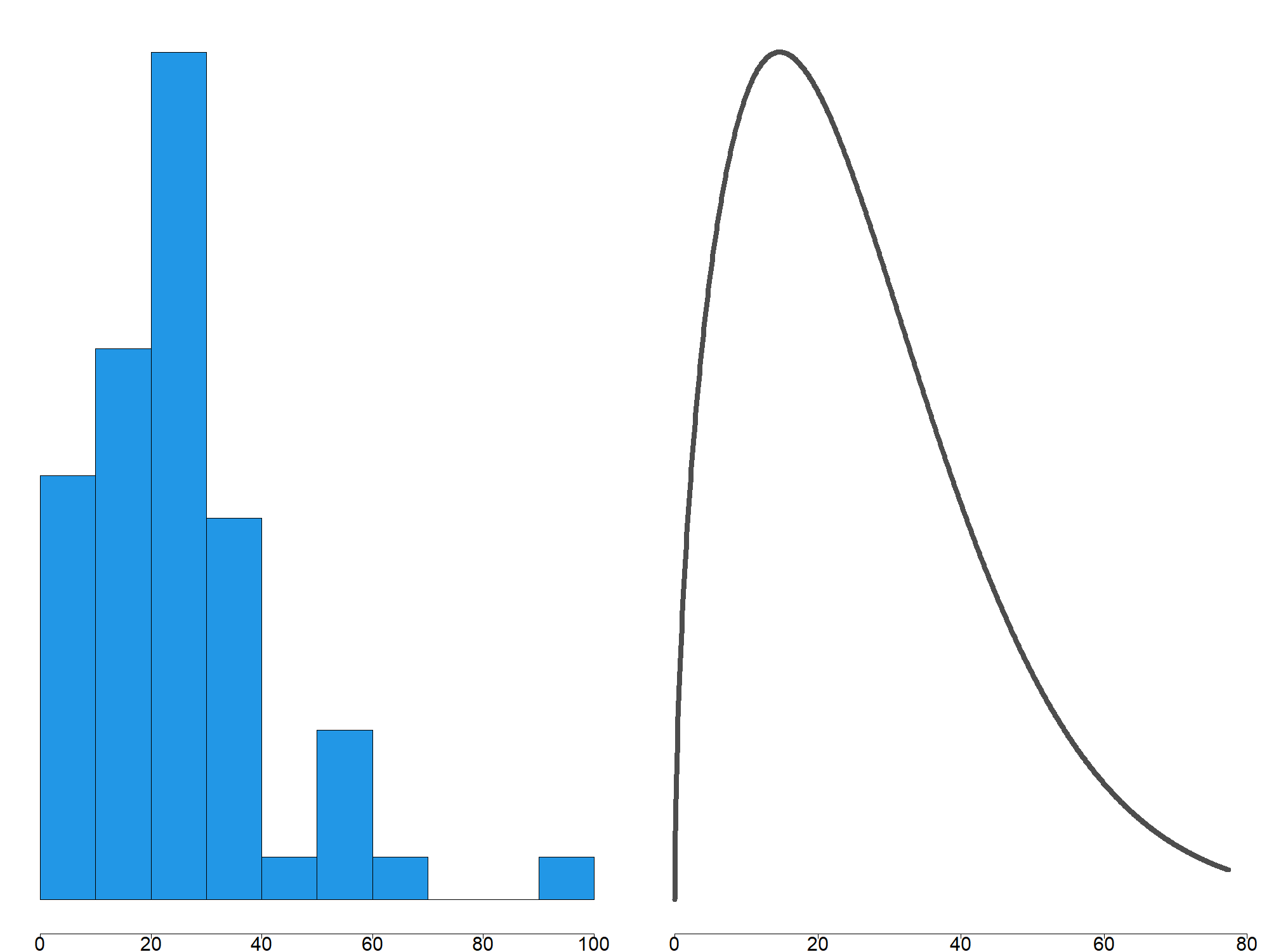
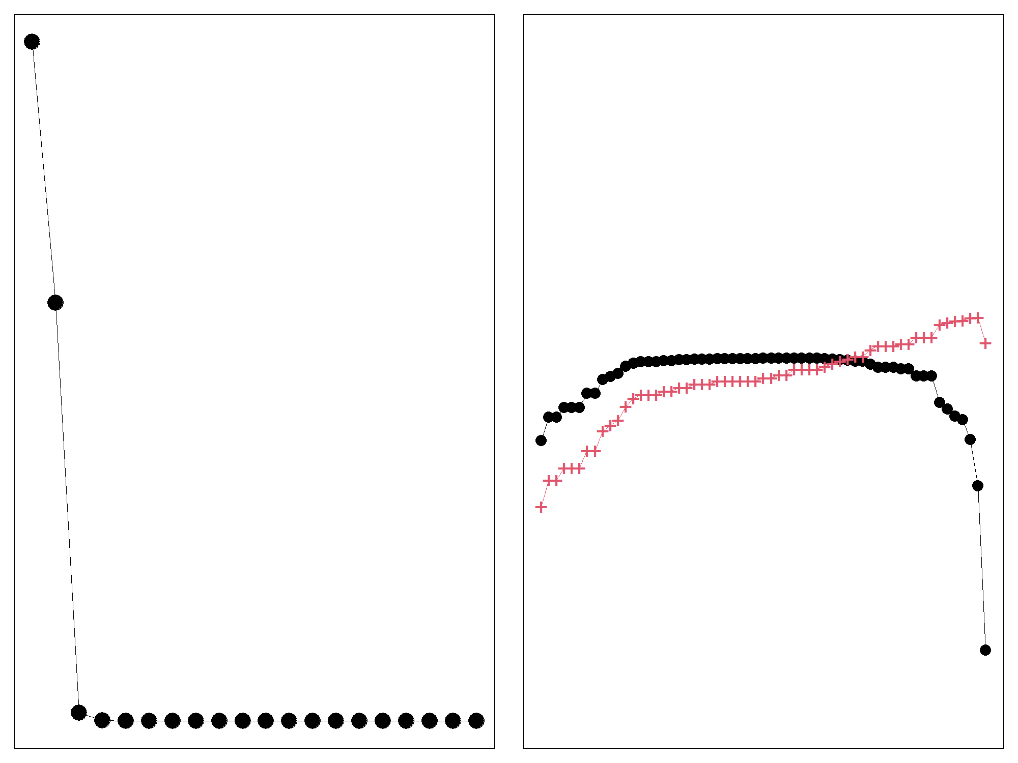
Figure 1. Weibull analysis. From the left to right, the first and second panel shows a histogram and a Weibull fitting (MLE) of the data, respectively. The third panel shows the first 20 eigenvalues of $W$ in a decreasing order; horizontal axis is the index $1\ldots 59$ of the eigenvalues. The fourth panel shows the eigenvectors corresponds to the first two eigenvalues; horizontal axis is the index $1\ldots 59$ of the observations. The black dot correspond to the first eigenvalue, while the red $+$ correspond to the second eigenvalue.

The results are shown in the third and fourth panels in Fig. 1. In the third panel, the first 20 eigenvalues of the matrix $W$ is plotted. The first two eigenvalues has a large value, while others have negligible magnitudes. The dimension of the essential subspace is two in this case, which equals to the number of parameters estimated in the model. This is, of course, not a coincidence, and will be explained in Sec. 4.3.

The normalized eigenvectors corresponds to these two eigenvalues are plotted in the fourth panel against the index of the observations. The amplitude of the eigenvector corresponding to the first eigenvalue takes a large value at high extreme of age, which agree with the an initiative impression that the estimate should be sensitive to this part of the data.

Regression

Next, we consider an example of the regression. A set of the artificial data is generated by

(36) $$Y_{i}=f(x_{i})+\widetilde{\sigma}\zeta_{i},\,\,\,\,\zeta_{i}\sim t_{4},\,\,\,\,i=1,\ldots,n,$$

where $t_{4}$ is the t-distribution of the degree 4 of freedom and we denote observations as $Y^{n}=(Y_{i})$ instead of $X^{n}=(X_{i})$ in the generic framework; here as usual $x_{i}$ indicates the value of the explanatory variables. Note that the t-distribution of the degree 4 of freedom is intentionally introduced to create outliers for a normal model defined below. We use a trigonometric curve as a true function $f(x)$ and set $n=30$ and $\widetilde{\sigma}=0.3$ in the following.

To this data set, we apply a Bayesian linear regression with a cubic polynomial

(37) $$Y_{i}\sim N(\mu_{i},\sigma^{2}),\,\,\,\mu_{i}=\beta_{0}+\beta_{1}x_{i}+\beta_{2}x_{i}^{2}+\beta_{3}x_{i}^{3},\,\,\,\,i=1,\ldots,n,$$

where an improper prior uniform on $(-\infty,\infty)$ is assumed for each coefficient $\beta_{\alpha},\,\,\alpha=0,\dots,3$. Also, an improper prior uniform on $[0,\infty)$ is assumed for the standard deviation $\sigma$ when we estimate $\sigma$ from the data. When $\sigma$ is given, we set $\sigma=0.1$. Below, the $\sigma$-given and $\sigma$-estimated case employ the same set of artificial data.

The result is shown in Fig. 2. The first panel shows data points used in the experiment (blue dot) and the fitted curve. The second panel shows the eigenvalues in the $\sigma$-given case; there are four nonzero eigenvalues and others are effectively zero, which agree with the number 4 of the estimated parameters. On the other hand, the third panel shows the eigenvalues in the $\sigma$-estimated case; it suggests five or six definitely nonzero eigenvalues, while the number of the estimated parameters is five. The cut off in this case is, however, rather ambiguous; this may be caused by the non-linearity in the estimation of the dispersion parameter $\sigma$.

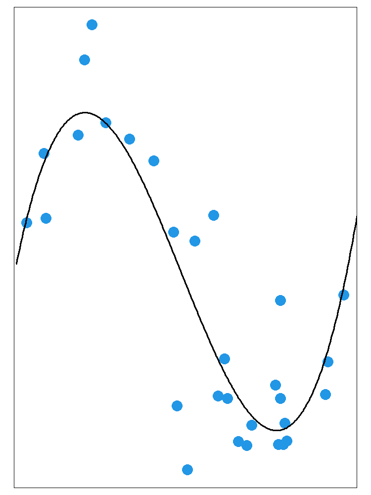
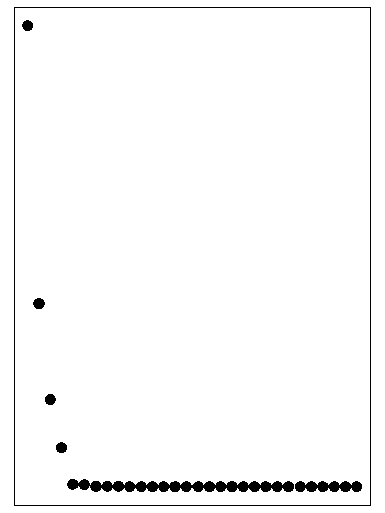
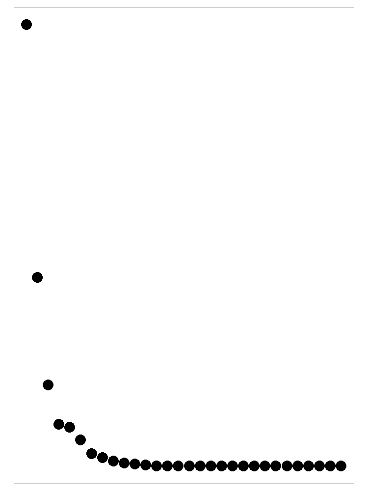
Figure 2. Regression. The first panel shows data points used in the experiment (blue dot) and the fitted curve; the horizontal axis shows $x$, while the verical axis shows $Y_{i}$ and the posterior mean of $f(x)$. The second and third panel shows the eigenvalues in the $\sigma$-given and $\sigma$-estimated case; the horizontal and vertical axis shows an index of eigenvalues and eigenvalues, respectively.

Smoothing

The third example employs a more structured model for time-series data. Let us consider a celebrated “Prussian horse kick data” $X_{tj},\,t=1,\ldots 20,\,j=1,\ldots 14$; this is a record of deaths by the horse kick during 20 years of 14 corps in the Prussian army.

We treat it as a time-series of the length 20 with 14 observations each year and apply a state space model with hidden Markov states $Z_{t},t=1,\ldots,20$, where a random walk of the state is assumed as a smoothness prior (a local-level model):

(38) $$Z_{t}=Z_{t-1}+\zeta_{t},\,\,\,t=2,\ldots,20.$$

The system noise $\zeta_{t}$ is an independent variate that obeys a common normal distribution $N(0,s^{2})$; improper priors uniform in $(-\infty,\infty)$ and $(0,\infty)$ are applied for the initial value $Z_{1}$ and the standard deviation $s$ of the system noise, respectively. On the other hand, each observation $X_{tj}$ is assumed to be an independent Poisson variate that obeys

(39) $$X_{tj}\sim Pois(\exp(Z_{t})),\,\,\,t=1,\ldots,20,\,\,j=1,\ldots,14,$$

where $Pois(\mu)$ denotes the Poisson distribution of the intensity $\mu$.

For a structured model, which part of the model is identified as the likelihood is important; the matrix $W$ depends on this choice. Here, we define the likelihood by (38) and identify $Z_{t}$ as the parameter $\theta$ in the generic framework; the state equation (39) is considered as a prior for $(Z_{t})$ together with an improper prior on $Z_{1}$. Total number of the observations is $20\times 14=280$, then $W$ becomes a $280\times 280$ matrix, which has 280 eigenvalues.

The result is shown in (3). The left panel shows the fitted curve. The right panel shows the first 30 eigenvalues. The number of definitely nonzero eigenvalues is 20, while the nominal number of the parameters is 21. The magnitude of the eigenvalue $\lambda_{i}$, however, smoothly decreases from $i=1$ to $i=20$; in that sense the subspace corresponding to the first 5 or 10 eigenvalues may be enough for the crude approximations.

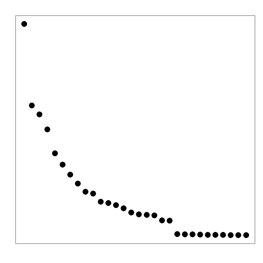
Figure 3. Smoothing. The left panel shows the fitted curve; the horizontal axis corresponds to the year $t=1,\ldots,20$, while the vertical axis corresponds to the posterior mean of $exp(Z_{t})$. The estimated curve is not smooth, because the prior penalizes the first-order difference. The right panel shows the first 30 eigenvalues; the horizontal and vertical axis shows an index of eigenvalues and eigenvalues, respectively.

4. W-kernel

This section defines the W-kernel; the essential subspace defined in the previous section is reformulated as a principal space defined by the kernel PCA with this kernel. Then, we discuss an approximation, here termed as modified Fisher kernel, which connects our approach to existing studies on natural kernels, such as the Fisher kernel and neural tangent kernels. Using this, we explain how the duality in the kernel PCA is interpreted in the light of W-kernel. Finally, we discuss the role of “centering”, typically expressed by a difference between the formulae (12) and (13); our argument also elucidates the effect of informative priors in the Bayesian IJK.

4.1. Basic definitions

Empirical version

Let us introduce an empirical version of the W-kernel as

(40) $$K_{W}(y,y^{\prime})=n\,\mathrm{Cov}_{\mathrm{pos}}[\ell(y;\theta),\ell(y^{\prime};\theta)]=n\,\mathrm{Cov}_{\mathrm{pos}}[\log p(y;\theta),\log p(y^{\prime};\theta)].$$

The sample size $n$ is introduced to the right hand side, because $\mathrm{Cov}_{\mathrm{pos}}[\ell(y;\theta),\ell(y^{\prime};\theta)]=O_{p}(1/n)$ holds in a usual setting.

A feature vector is defined as

(41) $$\Phi_{\theta}(X)=\ell(X;\theta)=\log p(X;\theta),$$

where a continuous-valued parameter $\theta$ plays the role of the index of features. An inner product is also defined by using the posterior covariance as

(42) $$(f,g)_{\mathcal{H}}=n\,\mathrm{Cov}_{\mathrm{pos}}[f(\theta),g(\theta)],$$

between any functions $f$ and $g$ of $\theta$ that can be regarded as posterior random variables. Note that it is positive-definite by the definition of the covariance.

Using this inner product, the reproducing kernel Hilbert space (RKHS) is given as a inner-product space defined by the closure of linear combinations of the form

(43) $$\sum_{i=1}^{k}c_{i}\log p(y_{i};\theta),$$

where $m$ is an arbitrary integer; $\{c_{i}\},\,i=1,\ldots,m$, is an arbitrary set of real numbers; $\{y_{i}\},\,i=1,\ldots,m$, is an arbitrary set of the possible observations.

Note that $k$ is not the dimension of the feature vector $\Phi_{\theta}(\cdot)$, but that of its index vector $\theta$; the feature vector itself is infinite-dimensional. This contrast with the modified Fisher kernel defined later (and also the Fisher kernel), where the feature vector is $k$-dimensional.

Population version

When we consider $K_{W}(X_{i},X_{j})$ using the definition (40) of the kernel, the same set $X^{n}=(X_{i})$ of observations is also used to define the inner product (42). Such a “data-dependent” definition of the kernel functions is rather familiar in the actual implementation of the kernel methods and also appeared in the usage of the Fisher kernel as discussed later.

However, it may be convenient to define a population version $K^{0}_{W}(X_{i},X_{j})$ of the W-kernel, where the inner product is independent of the current observations. We cannot directly use it in actual data analysis, but the results obtained by using $K_{W}(X_{i},X_{j})$ is interpreted as an empirical approximation to those had been obtained by the population version $K^{0}_{w}(X_{i},X_{j})$.

To do this, we need a frequencist’s assumption that observations are an IID realization from a population $G$. Then, a population version of the posterior with a sample size $n$ is formally introduced as

(44) $$p(\theta;G,n)=\frac{\exp\{n\int\ell(x;\theta)dG(x)\}p(\theta)}{\int\exp\{n\int\ell(x;\theta^{\prime})dG(x)\}p(\theta^{\prime})d\theta^{\prime}}.$$

Note that we recover the original posterior (3) when $dG(x)$ is replaced by the empirical version $d\hat{G}_{n}=(1/n)\sum_{i=1}^{n}\delta_{X_{i}}$ with point measures $\delta_{X_{i}}$ on observations $X^{n}=(X_{1},X_{2},\ldots,X_{n})$.

An advantage of the definition (44) is that the MAP estimate defined by the posterior (44) satisfies the population version of an estimating equation; see the equation (140) in the appendix B. It is a special case of the equation assumed in the theory of influence functions of M-estimators (Konishi and Kitagawa, (1996)).

If we denote a covariance with respect to the population version of the posterior (44) as $\mathrm{Cov}_{\mathrm{pos}}^{0}[\,\,,\,\,]$, we can define a population version of the W-kernel of the sample size $n$ as

(45) $$K^{0}_{W}(y,y^{\prime})=n\,\mathrm{Cov}^{0}_{\mathrm{pos}}[\ell(y;\theta),\ell(y^{\prime};\theta)]=n\,\mathrm{Cov}^{0}_{\mathrm{pos}}[\log p(y;\theta),\log p(y^{\prime};\theta)].$$

Kernel PCA

Now we can develop a kernel principal component analysis (kernel PCA; Schoelkopf and Smola, (2001); Shawe-Taylor and Cristianini, (2004)) using the W-kernel.

A way to introduce the kernel PCA is the maximization of the projection of a unit vector; here “projection” and “unit vactor” should be defined by the inner product of the RKHS. In our case, it reduces to the maximization of

(46) $$n^{2}\mathcal{F}(\varphi)=\sum_{i=1}^{n}(\varphi(\theta),\Phi_{\theta}(X_{i}))_{\mathcal{H}}^{2}=n^{2}\,\sum_{i=1}^{n}\left(\,\mathrm{Cov}_{\mathrm{pos}}[\varphi(\theta),\ell(X_{i};\theta)]\,\right)^{2}$$

with respect to

(47) $$(\varphi(\theta),\varphi(\theta))_{\mathcal{H}}=n\,\mathrm{Var}_{\mathrm{pos}}[\varphi(\theta)]=1.$$

$\mathcal{F}$ defined by (46) is the frequencist’s variance of $\mathbf{E}_{\mathrm{pos}}[\varphi(\theta)]$ in the light of the formula (13). Thus, our procedure is also interpreted as finding a projection that maximize the frequencist’s variance of the posterior mean.

If we introduce a Lagrange multiplier $\mu_{\varphi}$, it further reduces to the maximization of

(48) $$\widetilde{\mathcal{F}}(\varphi)=\sum_{i=1}^{n}\left(\,\mathrm{Cov}_{\mathrm{pos}}[\varphi(\theta),\ell(X_{i};\theta)]\,\right)^{2}-\mu_{\varphi}\mathrm{Var}_{\mathrm{pos}}[\varphi(\theta)].$$

Here we use a technique common in the kernel methods: According to the definition of the RKHS, we can expand $\varphi(\theta)$ as

(49) $$\varphi(\theta)=\sum_{i=1}^{n}v_{i}\ell(X_{i};\theta)$$

with unknown coefficients $(v_{i}),i=1,\ldots,n$. Substituting (49) in (48), a little calculation shows that it reduces to an eigenvalue problem of the matrix $W=(W_{ij})$ as

(50) $$\sum_{j=1}^{n}W_{ij}v_{j}=\sum_{j=1}^{n}\mathrm{Cov}_{\mathrm{pos}}[\ell(X_{i};\theta),\ell(X_{j};\theta)]v_{j}=\mu_{\varphi}v_{i},$$

which coincides with an eigenvalue problem that defines an essential subspace. A similar argument is also applied to the population version of the kernel $K^{0}_{W}(X_{i},X_{j})=\mathrm{Cov}_{\mathrm{pos}}^{0}[\ell(X_{i};\theta),\ell(X_{j};\theta)]$.

4.2. Relation to the Fisher kernel and neural tangent kernel

Fisher kernel

Jaakkola and Haussler, (1998) introduced a family of kernels induced from the likelihood functions, which they termed as the Fisher kernel (Schoelkopf and Smola, (2001); Shawe-Taylor and Cristianini, (2004); Zhang et al., (2022)). Kernels based on the likelihood functions are sometimes called as natural kernels (Schoelkopf and Smola, (2001)), which include the neural tangent kernel (Jacot et al., (2018)) recently introduced for the analysis of neural networks.

The Fisher kernel is regarded as a precursor of the W-kernel, in that both kernels are based on likelihood functions, but there is a more direct connection: As we will show in the following, the Fisher kernel is regarded as an approximation of the W-kernel when the model behind the kernel is regular and the effect of the prior can be ignored.

The Fisher kernel and other conventional natural kernels have a finite-dimensional feature space and easy to treat by analytical calculation, while our approach based on the posterior covariance has several advantages:

• The W-kernel is automatically computed from the posterior samples without model-by-model analytical calculation by hand. In this context, let us remind the readers that our start point is computational problems in Bayesian statistics, e.g., an efficient computation of the local case sensitivity and implementation of an approximate bootstrap with a single run of MCMC.

• It can includes the effect of the informative prior through the definition of the posterior covariance, which is automatically dealt in a MCMC computation; we will discuss it more in Sec. 4.4 and in the appendix B. This is in particular useful to treat structured models.

• The framework based on the W-kernel can be a hub to connect seemingly different fields of the research, such as local case sensitivity formulae, waic, the Fisher kernel, and stochastic expansion of the loss. We will also discuss a novel kind of Bayesian-frequencist’s duality in Sec. 4.3, which is only uncovered in the representation using the posterior covariance.

• The W-kernel can be defined for singular models, while other natural kernels limit to regular models because they rely on the score functions.

In general, a kernel approach should be designed to treat models in the data space, not in the feature-parameter space; the Fisher kernel and its generalizations, however, still invoke derivatives and a summation in the parameter space. The W-kernel minimizes the role of parameters both in definition and computation; it is by virtue of the Bayesian framework, where the parameters are only used to define the posterior covariance.

Approximation by a kernel with finite dimensional feature space

Let us consider an approximation of the W-kernel by a kernel with finite dimensional feature space. As a preparation, we will review a few well-used definitions and results in asymptotic theory. First, we define information matrices $\hat{\mathcal{J}}$ and $\mathcal{J}$ whose components are given by

(51) $$\hat{\mathcal{J}}_{\alpha\beta}=-\frac{1}{n}\sum_{i=1}^{n}\frac{\partial^{2}}{\partial\theta_{\alpha}\partial\theta_{\beta}}\ell(X_{i};\theta)\bigg{|}_{\theta=\hat{\theta}},\,\,\,\mathcal{J}_{\alpha\beta}=-\mathbf{E}_{X}\left[\left.\frac{\partial^{2}}{\partial\theta_{\alpha}\partial\theta_{\beta}}\ell(X;\theta)\right|_{\theta=\theta_{0}}\right],$$

where $\hat{\theta}=(\hat{\theta}_{\alpha})$ is the maximum likelihood estimate (MLE) from the data, and $\theta_{0}=(\theta^{0}_{\alpha})$ is a projection of the population onto the model (a quasi true-value), respectively. $\hat{\mathcal{J}}_{\alpha\beta}$ and $\mathcal{J}_{\alpha\beta}$ are regarded as an empirical and population version of the same quantity. If we denote an expectation with respect to the population version of the posterior (44) as ${\mathbf{E}}^{0}_{\mathrm{pos}}[\,\,\,]$, basic relations

(52) $$\mathbf{E}_{\mathrm{pos}}[(\theta_{\alpha}-\hat{\theta}_{\alpha})(\theta_{\beta}-\hat{\theta}_{\beta})] =\frac{(\hat{\mathcal{J}}^{-1})_{\alpha\beta}}{n}+o_{p}(1/n),$$

(53) $${\mathbf{E}}^{0}_{\mathrm{pos}}[(\theta_{\alpha}-\theta_{\alpha}^{0})(\theta_{\beta}-\theta_{\beta}^{0})] =\frac{(\mathcal{J}^{-1})_{\alpha\beta}}{n}+o_{p}(1/n)$$

hold, when we can ignore the effect of the prior and identify the MAP estimate with the MLE $\hat{\theta}$.

We also define another pair of information matrices $\hat{\mathcal{I}}$ and $\mathcal{I}$ as

(54) $$\hat{\mathcal{I}}_{\alpha\beta} =\frac{1}{n}\sum_{i=1}^{n}\left\{\frac{\partial}{\partial\theta_{\alpha}}\ell(X_{i};\theta)\bigg{|}_{\theta=\hat{\theta}}\frac{\partial}{\partial\theta_{\beta}}\ell(X_{i};\theta)\bigg{|}_{\theta=\hat{\theta}}\right\},\,\mathcal{I}_{\alpha\beta} =\mathbf{E}_{X}\left[\left.\frac{\partial}{\partial\theta_{\alpha}}\ell(X;\theta)\right|_{\theta=\theta_{0}}\left.\frac{\partial}{\partial\theta_{\beta}}\ell(X;\theta)\right|_{\theta=\theta_{0}}\right].$$

Again, they are an empirical and population version of the same quantity. The symbol $I$ is usually preferred but we use $\mathcal{I}$ to circumvent the confusion with the unit matrix. A classical result is that $\mathcal{I}=\mathcal{J}$ hold when the population $G$ represented by $p(x\mid\theta_{0})$. Also, asymptotically $\hat{\mathcal{I}}\simeq\hat{\mathcal{J}}$ under the same condition.

With these preparation, we will turn to the original problem. Here, we assume that the model behind the kernel is regular and parameterized by a finite number of the parameters, and also the effect of the prior can be ignored. Then, using (52), the W-kernel is approximated as

(55) $$K_{W}(y,y^{\prime})=n\,\mathrm{Cov}_{\mathrm{pos}}[\ell(y;\theta),\ell(y^{\prime};\theta)]$$

(56) $$=n\sum_{\alpha,\beta=1}^{k}\left\{\left.\frac{\partial}{\partial\theta_{\alpha}}\ell(y;\theta)\right|_{\theta=\hat{\theta}}\left.\frac{\partial}{\partial\theta_{\beta}}\ell(y^{\prime};\theta)\right|_{\theta=\hat{\theta}}\mathbf{E}_{\mathrm{pos}}[(\theta_{\alpha}-\hat{\theta}_{\alpha})(\theta_{\beta}-\hat{\theta}_{\beta})]\right\}+o_{p}(1)$$

(57) $$=\sum_{\alpha,\beta=1}^{k}\left\{\left.\frac{\partial}{\partial\theta_{\alpha}}\ell(y;\theta)\right|_{\theta=\hat{\theta}}\left.\frac{\partial}{\partial\theta_{\beta}}\ell(y^{\prime};\theta)\right|_{\theta=\hat{\theta}}(\hat{\mathcal{J}}^{-1})_{\alpha\beta}\right\}+o_{p}(1),$$

where $$k$$ is the number of the parameters. A similar calculation applied to the population version gives

(58) $$K^{0}_{W}(y,y^{\prime})=n\,\mathrm{Cov}^{0}_{\mathrm{pos}}[\ell(y;\theta),\ell(y^{\prime};\theta)]$$

(59) $$=\sum_{\alpha,\beta=1}^{k}\left\{\left.\frac{\partial}{\partial\theta_{\alpha}}\ell(y;\theta)\right|_{\theta=\theta_{0}}\left.\frac{\partial}{\partial\theta_{\beta}}\ell(y^{\prime};\theta)\right|_{\theta=\theta_{0}}(\mathcal{J}^{-1})_{\alpha\beta}\right\}+o_{p}(1).$$

Then, we define empirical and population versions of the approximate kernel as

(60) $$K_{MF}(y,y^{\prime}) =\sum_{\alpha,\beta=1}^{k}\left\{\left.\frac{\partial}{\partial\theta_{\alpha}}\ell(y;\theta)\right|_{\theta=\hat{\theta}}\left.\frac{\partial}{\partial\theta_{\beta}}\ell(y^{\prime};\theta)\right|_{\theta=\hat{\theta}}(\hat{\mathcal{J}}^{-1})_{\alpha\beta}\right\},$$

(61) $$K^{0}_{MF}(y,y^{\prime}) =\sum_{\alpha,\beta=1}^{k}\left\{\left.\frac{\partial}{\partial\theta_{\alpha}}\ell(y;\theta)\right|_{\theta=\theta_{0}}\left.\frac{\partial}{\partial\theta_{\beta}}\ell(y^{\prime};\theta)\right|_{\theta=\theta_{0}}(\mathcal{J}^{-1})_{\alpha\beta}\right\},$$

which approximate $K_{W}(y,y^{\prime})$ and $K^{0}_{W}(y,y^{\prime})$, respectively.

They are almost the same as the Fisher kernel introduced in Jaakkola and Haussler, (1998), whose empirical and population versions are given as

(62) $$K_{F}(y,y^{\prime}) =\sum_{\alpha,\beta=1}^{k}\left\{\left.\frac{\partial}{\partial\theta_{\alpha}}\ell(y;\theta)\right|_{\theta=\hat{\theta}}\left.\frac{\partial}{\partial\theta_{\beta}}\ell(y^{\prime};\theta)\right|_{\theta=\hat{\theta}}(\hat{\mathcal{I}}^{-1})_{\alpha\beta}\right\},$$

(63) $$K^{0}_{F}(y,y^{\prime}) =\sum_{\alpha,\beta=1}^{k}\left\{\left.\frac{\partial}{\partial\theta_{\alpha}}\ell(y;\theta)\right|_{\theta=\theta_{0}}\left.\frac{\partial}{\partial\theta_{\beta}}\ell(y^{\prime};\theta)\right|_{\theta=\theta_{0}}(\mathcal{I}^{-1})_{\alpha\beta}\right\}.$$

The only difference between them is that $\hat{\mathcal{I}}$ and $\mathcal{I}$ in (62), (63) are replaced by $\hat{\mathcal{J}}$ and $\mathcal{J}$ in (60), (61).

In some literature, the kernels (60), (61) are also called as the Fisher kernel, but we will call them modified Fisher kernel, because there will be considerable difference between (60), (61) and (62), (63) when the model is misspecified. When the population $G$ can be represented by $p(x\mid\theta_{0})$, $\mathcal{I}=\mathcal{J}$ hence (61) coincides with (63). Also, (60) and (62) are asymptotically the same in the same condition.

The modified Fisher kernel is defined by a sum of $k$ terms, while the W-kernel is defined by a $k$-fold integral, where the $k$ is the number of parameters. Then, we have a dimensional reduction and the ease of analytical treatment in (60) and (61), at the expense of the favorable properties from (i) to (iv) of the posterior covariance representation.

Finally, we note that these kernels are also closely related to the neural tangent kernel defined in Jacot et al., (2018). In its empirical form, it is given as

(64) $$K_{NTK}(y,y^{\prime})=\sum_{\alpha,\beta=1}^{k}\left\{\left.\frac{\partial}{\partial\theta_{\alpha}}\ell(y;\theta)\right|_{\theta=\hat{\theta}}\left.\frac{\partial}{\partial\theta_{\beta}}\ell(y^{\prime};\theta)\right|_{\theta=\hat{\theta}}\right\},$$

which contains neither $\hat{\mathcal{J}}$ nor $\hat{\mathcal{I}}$. This kernel is also called the plain kernel in Schoelkopf and Smola, (2001), where a generic form of natural kernels parameterized by a matrix $M$ is discussed; $M=\hat{\mathcal{I}}$ or $\mathcal{I}$ in the Fisher kernel, $M=\hat{\mathcal{J}}$ or $\mathcal{J}$ in the modified Fisher kernel, and $M$ equals to an identity matrix in the plain kernel.

Finite dimensional feature vectors

For the later convenience, we explicitly give a finite dimensional feature vector that corresponds to the modified Fisher kernels (60) and (61). Here, we define principal square roots $\hat{\mathcal{J}}^{-1/2}$ and $\mathcal{J}^{-1/2}$ of the matrices $\hat{\mathcal{J}}^{-1}$ and $\mathcal{J}^{-1}$ as positive-semidefinite matrices that satisfy

(65) $$\hat{\mathcal{J}}^{-1}_{\alpha\beta}=\sum_{\gamma=1}^{k}\hat{\mathcal{J}}^{-1/2}_{\alpha\gamma}\hat{\mathcal{J}}^{-1/2}_{\gamma\beta},\,\,\,\,\mathcal{J}^{-1}_{\alpha\beta}=\sum_{\gamma=1}^{k}\mathcal{J}^{-1/2}_{\alpha\gamma}\mathcal{J}^{-1/2}_{\gamma\beta}.$$

Then, the feature vectors corresponding to an empirical and population version of the modified Fisher kernel (60) and (61) are expressed as

(66) $$\Phi^{MF}(\gamma,y)=\sum_{\alpha=1}^{k}(\hat{\mathcal{J}}^{-1/2})_{\gamma\alpha}\frac{\partial}{\partial\theta_{\alpha}}\ell(y;\theta)\bigg{|}_{\theta=\hat{\theta}},\,\,\,\,\Phi^{MF}_{0}(\gamma,y)=\sum_{\alpha=1}^{k}(\mathcal{J}^{-1/2})_{\gamma\alpha}\frac{\partial}{\partial\theta_{\alpha}}\ell(y;\theta)\bigg{|}_{\theta=\theta_{0}}.$$

This already discussed in Schoelkopf and Smola, (2001), Section 13.4 and Oliver et al., (2000) for a generic form of the natural kernels. For the reader’s convenience, however, we sketch the derivation of (66) in the appendix A.3.

4.3. Duality via posterior covariance

Duality in the eigenvalue problem

Let us see the diagonal sum of the W-kernel divided by the sample size $n$; it is given by

(67) $$\frac{1}{n}\sum_{i=1}^{n}K_{W}(X_{i},X_{i})=\mathrm{tr\,}[W]=\sum_{i=1}^{n}\mathrm{Cov}_{\mathrm{pos}}[\ell(X_{i};\theta),\ell(X_{i};\theta)]=\sum_{i=1}^{n}\mathrm{Var}_{\mathrm{pos}}[\ell(X_{i};\theta)],$$

which coincides with the bias correction term of waic (Watanabe, (2010, 2018)). On the other hand, the diagonal sum of the modified Fisher kernel divided by the sample size $n$ is computed as

(68) $$\frac{1}{n}\sum_{i=1}^{n}K_{MF}(X_{i},X_{i}) =\frac{1}{n}\sum_{\alpha,\beta=1}^{k}\sum_{i=1}^{n}\left\{\left.\frac{\partial}{\partial\theta_{\alpha}}\ell(X_{i};\theta)\right|_{\theta=\hat{\theta}}\left.\frac{\partial}{\partial\theta_{\beta}}\ell(X_{i};\theta)\right|_{\theta=\hat{\theta}}\right\}(\hat{\mathcal{J}}^{-1})_{\alpha\beta}$$

(69) $$=\mathrm{tr\,}\left[\hat{\mathcal{I}}\hat{\mathcal{J}}^{-1}\right]=\mathrm{tr\,}\left[\hat{\mathcal{J}}^{-1/2}\hat{\mathcal{I}}\hat{\mathcal{J}}^{-1/2}\right].$$

It is known as the bias correction term of the tic (Takeuchi’s Information Criterion; Takeuchi, (1976); Konishi and Kitagawa, (2008)). Thus, we reproduce a known result that bias correction terms of waic and tic are asymptotically equivalent in regular models when the effect of the prior is neglected (Watanabe, (2018)).

The above-mentioned relation suggests that a symmetric matrix $\hat{\mathcal{J}}^{-1/2}\hat{\mathcal{I}}\hat{\mathcal{J}}^{-1/2}$ is closely related to the matrix $W$. In fact, the sets of non-zero eigenvalues of both matrices approximately matches with multiplicity for a regular model with a non informative prior. To express the relation precisely, we denote the eigenvalues of $\hat{\mathcal{J}}^{-1/2}\hat{\mathcal{I}}\hat{\mathcal{J}}^{-1/2}$ as $\lambda^{I}_{1}\geq\lambda^{I}_{2}\geq\cdots\geq\lambda^{I}_{k}$, and the eigenvalues of $W$ as $\lambda^{W}_{1}\geq\lambda^{W}_{2}\geq\cdots\geq\lambda^{W}_{n}$, where $k$ is the number of the parameters and $n$ is the number of observations. Assuming $n\gg k$ , the relation between them is given as follows:

(70) $$\lambda^{W}_{j}\simeq\lambda^{I}_{j}\text{ for $j\leq k$},\ \ \lambda^{W}_{j}\simeq 0\text{ for $k<j$}.$$

This relation explain why the number of virtually non-zero eigenvalues approximately equals to $k$ when $n\rightarrow\infty$.

The origin of (70) is that the eigenvalue problems of $K_{MF}(X_{i},X_{j})$ and $\hat{\mathcal{J}}^{-1/2}\hat{\mathcal{I}}\hat{\mathcal{J}}^{-1/2}$ is dual in the sense of the PCA. That is, the feature vector $\Phi^{MF}(\gamma,X_{j})$ defined by (66) satisfies a dual pair of relations

(71) $$\frac{1}{n}K_{MF}(X_{i},X_{j})=\frac{1}{n}\sum_{\gamma=1}^{k}\Phi^{MF}(\gamma,X_{i})\Phi^{MF}(\gamma,X_{j}).$$

(72) $$\left(\hat{\mathcal{J}}^{-1/2}\hat{\mathcal{I}}\hat{\mathcal{J}}^{-1/2}\right)_{\gamma\delta} =\frac{1}{n}\sum_{i=1}^{n}\Phi^{MF}(\gamma,X_{i})\Phi^{MF}(\delta,X_{i}).$$

Since both of (71) and (72) have a form of the Euclidean inner product, an argument standard for the duality in PCA gives the relation

(73) $$\lambda^{MF}_{j}=\lambda^{I}_{j}\text{ for $j\leq k$},\ \ \lambda^{MF}_{j}=0\text{ for $k<j$},$$

when we denote the eigenvalues of $\frac{1}{n}K_{MF}(X_{i},X_{j})$ as $\lambda^{MF}_{i}$, which are ordered as $\lambda^{MF}_{1}\geq\lambda^{MF}_{2}\geq,\cdots,\lambda^{MF}_{k}$. Again, these arguments are essentially given in Schoelkopf and Smola, (2001) and Oliver et al., (2000). The derivation of (71) and (72) is also given in the appendix A.3.

Let us return to the issues on the W-kernel. The matrix $W$ equals to $\frac{1}{n}K_{W}(X_{i},X_{j})$. Thus, if the kernel $K_{W}$ is well approximated by the kernel $K_{MF}$, the relation (73) for $\frac{1}{n}K_{MF}(X_{i},X_{j})$ implies the relation (70) for the W-matrix, which completes our derivation. It also gives an explanation on the apparent instability of the eigenvectors that span an essential subspace; this reflects a common property of the dual PCA in the data space when $n\gg k$.

Remark 7.

When $n\leq k$, the relation $\lambda^{I}_{j}=\lambda^{MF}_{j}\text{\ for $j\leq n$},\ \lambda^{I}_{j}=0\text{\ for $n<j$},$ holds, but it does not necessarily give the corresponding relation for $\lambda^{W}_{j}$s, because an asymptotic relation $\lambda^{I}_{j}\simeq\lambda^{MF}_{j}$ may not hold in this case.

Bayesian-Frequencist’s duality

In essence, the duality between the W-kernel $K_{W}$ and $\hat{\mathcal{J}}^{-1/2}\hat{\mathcal{I}}\hat{\mathcal{J}}^{-1/2}$ is a rephrase of the one between the modified Fisher kernel $K_{MF}$ and $\hat{\mathcal{J}}^{-1/2}\hat{\mathcal{I}}\hat{\mathcal{J}}^{-1/2}$. An interpretation via posterior covariance provides, however, interesting results such that an equality between the bias correction terms of waic and tic is interpreted as an equality between the sum of diagonals of the dual pair of the matrices.

Here, we will add one more subject that is only shown up in the posterior covariance representation. Take a look at representations of the inner products in a pair of the dual spaces. It is expressed as a posterior covariance in the data space. On the other hand, the formula (72) implies that it is expressed by the sum over the observations $X_{i}$ in the feature space (or parameter space) when we consider the approximation with the modified Fisher kernel. To clarify the contrast, let us shift to the population version and represent (72) as a population average; we have

(74) $$(\Phi_{\theta}(X),\Phi_{\theta}(X^{\prime}))_{\mathrm{pos}} =n\mathrm{Cov}_{\mathrm{pos}}^{0}[\ell(X;\theta),\ell(X^{\prime};\theta)]$$

(75) $$\Leftrightarrow\,\,\,(\Phi^{MF}(\gamma,X),\Phi^{MF}(\delta,X))_{d}=n\mathbf{E}_{X}[\Phi^{MF}(\gamma,X)\Phi^{MF}(\delta,X)],$$

where we denote the inner product in the feature space as $$(\,\,,\,\,)_{d} \Leftrightarrow \mathbf{E}_{X}[\Phi^{MF}(\gamma,X)]$$, and the arrow “” shows a comparison between the inner products schematically. As shown in the appendix A.3, the population average is always zero, then we can also express the above as

(76) $$(\Phi_{\theta}(X),\Phi_{\theta}(X^{\prime}))_{\mathrm{pos}} =n\mathrm{Cov}_{\mathrm{pos}}^{0}[\ell(X;\theta),\ell(X^{\prime};\theta)]$$

(77) $$\Leftrightarrow\,\,\,(\Phi^{MF}(\gamma,X),\Phi^{MF}(\delta,X))_{d}=n\mathrm{Cov}_{X}[\Phi^{MF}(\gamma,X),\Phi^{MF}(\delta,X)].$$

Above relations imply a Bayesian-Frequencist’s duality given as follows:

• The left hand side of “$\Leftrightarrow$” : Inner product in the data space is represented by the posterior covariance $\mathrm{Cov}_{\mathrm{pos}}^{0}[\,\,\,\,]$, which is a genuine Bayesian quantity.

• The right hand side of “$\Leftrightarrow$”: Inner product in the feature space is represented by the frequencist’s covariance $\mathrm{Cov}_{X}[\,\,\,\,]$, which is defined by a repeated sampling from the population.

It seems a distinct property of the proposed kernel framework to reveal such a relation; the inner product in the data space is formulated in this style only through the posterior covariance interpretation.

Information geometry

Another interesting subject here is a connection to the information geometry. In view of the information geometry, the feature vectors defined by (66) is considered as a basis of a tangential space equipped with the inner product $(\Phi^{MF}(\gamma,X),\Phi^{MF}(\delta,X))_{d}$. That is, the right hand side of “$\Leftrightarrow$” belongs to the world of the conventional information geometry (Schoelkopf and Smola, (2001), Section 13.4).

Then, how about the left hand side of “$\Leftrightarrow$” ? It will be interesting to interpret it as a “data space representation” of the geometry of a statistical model. Then, the essential subspace defined in this paper plays the role of a tangential space in the information geometry. An advantage of using a posterior covariance in the left hand side is that it may apply in the settings where conventional information geometry meets difficulty, such as the case with singular models.

4.4. Centering and informative priors

Centering and double centering

So far, we ignore the difference between the original form (12) and the simplified form (13) of the frequencist’s covariance formulae. This difference is realized by replacing the posterior covariance $\mathrm{Cov}_{\mathrm{pos}}$ to a “centered” form $\mathrm{Cov}_{\mathrm{pos}}^{*}$ defined by

(78) $$\mathrm{Cov}_{\mathrm{pos}}^{*}[A(\theta),\ell(X_{i};\theta)]=\mathrm{Cov}_{\mathrm{pos}}[A(\theta),\ell(X_{i};\theta)]-\frac{1}{n}\sum_{j=1}^{n}\mathrm{Cov}_{\mathrm{pos}}[A(\theta),\ell(X_{j};\theta)],$$

where $A(\theta)$ is an arbitrary statistics; (78) is already appeared as (11), but reproduced here for the reader’s convenience.

On the other hand, Kernel PCA often utilizes the “double-centered” version $\widetilde{K}$ of the kernel $K$, which is defined as

(79) $$\widetilde{K}(X_{i},X_{j})=K(X_{i},X_{j})-\frac{1}{n}\sum_{m=1}^{n}K(X_{i},X_{m})-\frac{1}{n}\sum_{l=1}^{n}K(X_{l},X_{j})-\frac{1}{n^{2}}\sum_{l,m=1}^{n}K(X_{l},X_{m}).$$

In the case of W-kernel, this modification corresponds to the use

(80) $$\widetilde{K}_{W}(X_{i},X_{j})=n\,\mathrm{Cov}_{\mathrm{pos}}\left[\ell(X_{i};\theta)-\frac{1}{n}\sum_{m=1}^{n}\ell(X_{m};\theta)\,\,,\,\,\ell(X_{j};\theta)-\frac{1}{n}\sum_{m=1}^{n}\ell(X_{m};\theta)\right]$$

instead of $K_{W}$. Then, the use of the “centered” form $\mathrm{Cov}_{\mathrm{pos}}^{*}$ is equivalent to the double centering of the W-kernel in our kernel framework.

Rationale for centering

A natural way to understand the meaning of centering in the definition (78) is in the context of influence functions. When we define the first-order influence functions $T^{(1)}(x,G)$, we usually assume $\mathbf{E}_{X}[T^{(1)}(x,G)]=0$, where $\mathbf{E}_{X}$ denotes an average over the population $G$. This condition allows simplifications of related formulae, such as from $\mathrm{Var}_{X}[T^{(1)}(x,G)]$ to $\int\{T^{(1)}(x,G)\}^{2}dG(x)$ for frequencist’s variance. On the other hand, an origin of the relation $\mathbf{E}_{X}[T^{(1)}(x,G)]=0$ may be traced back to the fact that influence functions are defined for the changes in a probability distribution $G$ that satisfy $\int dG(x)=1$; this corresponds to the condition $\sum_{i=1}^{n}w_{i}=1$ in the definition of the weighted posterior (5).

Note that, however, the centering in (78) will not be necessary, or even harmful, in some cases. For example, when we are interested in sensitivity analysis, as in Sec. 3.1 and Sec. 3.2, it may not be adequate to assume the constraints $\sum_{i=1}^{n}w_{i}=1$. In these cases, there are no reason for the centering (78). On the other hand, in the approximate bootstrap discussed in Sec. 5.2, the condition $\sum_{i=1}^{n}w_{i}=1$ is explicitly satisfied; in this case, it is easy to see that neither of the centering and double centering do not affect the result.

In practice, it is important to note that the centering is only effective in the case of considerably strong priors; see numerical experiments in the appendix B.1. We will discuss how and why this goes in the rest of this subsection, which also elucidates the effect of informative priors in the Bayesian IJK.

$O(1)$ priors

First, we consider the case that the prior is not dependent to the sample size $n$; hereafter we call this setting as $O(1)$ priors. In this case, the effect of the centering is asymptotically negligible for a large $n$, that is,

(81) $$\frac{1}{n}\sum_{i=1}^{n}\mathrm{Cov}_{\mathrm{pos}}[A(\theta),\,\ell(X_{i};\theta)]=\mathrm{Cov}_{\mathrm{pos}}\left[A(\theta),\,\frac{1}{n}\sum_{i=1}^{n}\ell(X_{i};\theta)\right]=o_{p}(1/n)$$

holds in (78), while the first term in (78) is $O_{p}(1/n)$. An initiative argument to justify (81) is given in the appendix A.4; in a nutshell, it is caused by the posterior concentration around the MLE $\hat{\theta}$ that satisfies $\sum_{i=1}^{n}\ell(X_{i};\hat{\theta})=0$.

$O(n)$ priors

In the setting of $O(1)$ prior, the effect of the prior usually vanishes in $n\rightarrow\infty$ for regular models. To quantify the effect of the prior more precisely, “$O(n)$ setting” is introduced in the literature (Konishi and Kitagawa, (2008); Ninomiya, (2021)), where the magnitude of the prior is intensified as $O(n)$ in the $n\rightarrow\infty$ limit; hereafter we call it as $O(n)$ priors. To be explicit, we define

(82) $$\log p(\theta)=n\Lambda\log\widetilde{p}(\theta)+\log p_{0}(\theta)+c$$

with densities $\widetilde{p}(\theta),p_{0}(\theta)$, and constants $\Lambda$ and $c$. The first term $n\Lambda\log\widetilde{p}(\theta)$ is the main term that represents an informative prior. A little ingenuity of us is that we introduce a constant $\Lambda$ to control the strength of the informative prior. $p_{0}(\theta)$ is a “base prior”, which is added only for the formal purpose and often neglected hereafter. The constant $c$ is added for the normalization of $p(\theta)$. We keep the number of the parameters constant when $n\rightarrow\infty$ as in the classical setting of $O(1)$ priors.

Under the assumption of the $O(n)$ prior, we have the following observations:

• The original formula (12) with centering gives an asymptotically correct estimate of the frequencist’s covariance even in the $O(n)$ setting.

• The simplified formula (13) without centering does not give an asymptotically correct estimate of the frequencist’s covariance in the $O(n)$ setting; in other words, $n$ times (13) is not a consistent estimator of $n$ times the frequencist’s covariance.

• However, the difference between (12) and (13) is $O_{p}(\Lambda^{2})$ when we ignore $o_{p}(1/n)$ terms; it is different from $O_{p}(\Lambda)$ that we naively expect. When $\Lambda$ is small, this results in a considerably smaller correction compared with cases where the difference is $O_{p}(\Lambda)$.

The property (a) is a natural consequence of the concentration of posterior measure in the $O(n)$ setting; a generalization of the heuristic argument in Sec.2.1 of Giordano and Broderick, (2023) to $O(n)$ priors is given in the appendix B.2. Derivations of the properties (b) and (c) are given in the appendix B.3.

The properties (a) and (b) will be widely applied in applications of the Bayesian IJK that are based on (78). On the other hand, the third property (c) is specific to the application to the frequencist’s covariance and not directly explained in the relations (78); a similar property also hold for the bias correction term of waic (see the appendix B.4), but it may not hold in other outcome of the Bayesian IJK.

These properties give a qualitative support to the intuition that the Bayesian IJK includes the effect of the prior, despite it is informed on the prior only though the definition of the posterior mean. The centering in (78) improves the results for an informative prior, but it captures considerable amount of the prior information even without the centering, as seen in the fact that the difference between (12) and (13) is $O(\Lambda^{2})$.

Alternative form of frequencist’s covariance formula

Finally, we remark that (78) is asymptotically equivalent to the following expression in the setting of $O(n)$ priors:

(83) $$\mathrm{Cov}_{\mathrm{pos}}^{**}[A(\theta),\ell(X_{i};\theta)] =\mathrm{Cov}_{\mathrm{pos}}\left[A(\theta),\ell(X_{i};\theta)+\frac{1}{n}\log p(\theta)\right],$$

which leads to another estimator of the frequencist’s covariance:

(84) $$\hat{\Sigma}^{**}_{AB} =\sum_{i=1}^{n}\,{\mathrm{Cov}_{\mathrm{pos}}\left[A(\theta),\ell(X_{i};\theta)+\frac{1}{n}\log p(\theta)\right]\,\mathrm{Cov}_{\mathrm{pos}}\left[B(\theta),\ell(X_{i};\theta)+\frac{1}{n}\log p(\theta)\right].}$$

The definition (83) has a form that $1/n$ of the log-prior is added to the log-likelihood of each observation, which looks intuitively reasonable modification for informative priors.

To show the asymptotic equivalence, we start from a relation that holds for $O(n)$ priors:

(85) $$\mathrm{Cov}_{\mathrm{pos}}\left[A(\theta),\sum_{i=1}^{n}\left\{\ell(X_{i};\theta)+\frac{1}{n}\log p(\theta)\right\}\right]=o_{p}(1).$$

As seen in the appendix A.4, the relation (85) is a generalisation of (81) to the case with $O(n)$ priors; the relation (81) itself does not hold in the setting of $O(n)$ priors.

Using (85), we have

(86) $$-\frac{1}{n}\sum_{i=1}^{n}\mathrm{Cov}_{\mathrm{pos}}\left[A(\theta),\ell(X_{i};\theta)\right]=\mathrm{Cov}_{\mathrm{pos}}\left[A(\theta),\frac{1}{n}\log p(\theta)\right]+o_{p}(1/n),$$

which leads to the asymptotic equivalence between (11) and (83).

Remark 8.

The modification (83) is already discussed in Iba and Yano, (2022) under the context of information criteria. In general, the effect of $O(n)$ priors in model selection is studied in Konishi and Kitagawa, (1996), Vehtari et al., (2017), and Ninomiya, (2021). We will discuss more on this issue in Sec.  B.4.

5. Applications

In this last section, two applications of the proposed framework are shown. These examples make us return to the issues addressed at the beginning of this paper: sensitivity analysis and assessment of the Bayesian estimates by bootstrap replication of the observations. We will also discuss here more on computational aspects, which have not been examined enough in the previous sections.

5.1. Selecting a representative set of observations

In this subsection, we introduce the incomplete Cholesky decomposition as a tool to obtain essential subspace, which naturally leads to the notion of a representative set of observations.

Incomplete Cholesky decomposition

Incomplete Cholesky decomposition developed in machine learning is an algorithm applied to a positive-semidefinite symmetric matrix; it is often used in kernel methods to treat a large Gram matrix. In our case, it corresponds to the decomposition

(87) $$W=P(LL^{T}+R)P^{T},$$

where $L$ is a lower triangular matrix that satisfies $L_{ij}=0$ for $j>\widetilde{a}_{M}$, $P$ is a permutation matrix, and $R$ is a residual.

Incomplete Cholesky decomposition is computed in a sequential way with a greedy choice of the pivot at each step (Shawe-Taylor and Cristianini, (2004); the permutation matrix $P$ is determined by these choices in a post hoc way. The diagonal sum $\mathrm{tr\,}R$ is monitored in each step as an index of residuals (residual variance), and when it becomes a negligible value, we stop the procedure and regard $P(LL^{T})P^{T}$ as an approximation of $W$ that has enough precision to represent the essential subspace. The number of non-zero column $\widetilde{a}_{M}$ of $L$ is determined by this procedure. Required computation is in the order of $O(\widetilde{a}_{M}^{2}\times n)$.

Hereafter, we assume the following three to save the notations: (i) The rows and columns of the matrix $W$ are already sorted simultaneously in a way that $P$ becomes an identity matrix, (ii) The residual $R$ is negligible and can be omitted in a formula, (iii) $\widetilde{a}_{M}=a_{M}$. For (iii), $\widetilde{a}_{M}$ is usually larger than $a_{M}$ for the same value of the residual variance because $a_{M}$ corresponds to the optimal orthogonal basis, but for simplicity we apply the same notation to them.

Assuming (i) and (ii), the definition (87) is simplified to $W=LL^{T}$. In Fig. 4, the relation $W=LL^{T}$ and its dual form $L^{T}L$ is graphically expressed.

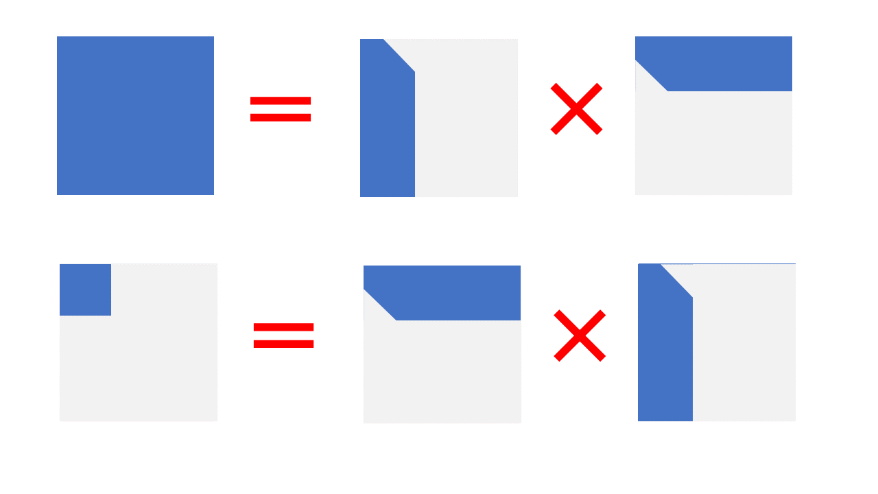
Figure 4. Schismatic view of the incomplete Cholesky decomposition. Upper panel shows $W=LL^{T}$, while lower panel shows the result of $L^{T}L$. Non-zero components of each matrix belong to the dark-color regions, while the light-color regions are filled with zero. The symbol “$\times$” means a matrix product. We assume the row and column of the matrix $W$ is already sorted and neglect the residual; see the main text for details.

With these preparations, let us consider an eigenvalue problem of the matrix $L^{T}L$ as

(88) $$(L^{T}L)V_{a}=\lambda^{\mathrm{v}}_{a}V_{a}.$$

Here and hereafter, we assume $V_{a}$ has a unit length and hence $\bm{V}=(V_{a})$ is an orthogonal matrix. A generic form of $L^{T}L$ is a $a_{M}\times a_{M}$ dense symmetric matrix, which has eigenvalues $\lambda^{\mathrm{v}}_{a},\,a=1,\ldots,a_{M}$. $O(a_{M}^{3})$ computation is enough to solve this eigenvalue problem.

Multiplying $L$ to both hand side of (88), we have

(89) $$L(L^{T}L)V_{a}=\lambda^{\mathrm{v}}_{a}LV_{a}.$$

Since $LL^{T}=W$, the above is rewritten as

(90) $$W(LV_{a})=\lambda^{\mathrm{v}}_{a}(LV_{a})$$

This shows that $\lambda^{\mathrm{v}}_{a},\,a=1,\ldots,a_{M}$ equal to the set of non-zero eigenvalues of $W=LL^{T}$; other eigenvalues of $W$ are (almost) zero. Also, an eigenvector of $W$ corresponding to $\lambda^{\mathrm{v}}_{a}$ is given by $LV_{a}$. A unit eigenvector is obtained as

(91) $$\widetilde{U}_{a}=LV_{a}\big{/}\sqrt{\lambda^{\mathrm{v}}_{a}},$$

because $\widetilde{U}^{T}_{a}\widetilde{U}_{a}=V^{T}_{a}L^{T}LV_{a}/\lambda^{\mathrm{v}}_{a}=1$. It requires $O(a_{M}\times n)$ computation to obtain a unit eigenvector for each $a$ and $O(a_{M}^{2}\times n)$ for all eigenvectors corresponding to effectively non-zero eigenvalues.

Representative set of the observations

Up to now, we consider incomplete Cholesky decomposition as an efficient computational method to solve a large eigenvalue problem. As already noticed, it is in itself useful, because it gives a minimum set of the observations that can effectively represent any perturbation to the data.

To see this, let us define

(92) $$\widetilde{\eta}^{\dagger}_{b}=\sum_{i=1}^{n}L^{T}_{bi}\eta_{i},\,b=1,\ldots,a_{M}.$$

Since we assume that the matrix $W$ are already sorted in a way that the permutation $P$ becomes an identity matrix, the set of indices $b=1,\cdots,a_{M}$ corresponds to the observations selected by the incomplete Cholesky decomposition. Using (91) and (92), $\widetilde{\eta}_{a}$ defined in the equations (19) and (32) is expressed as

(93) $$\widetilde{\eta}_{a}=\sum_{i=1}^{n}U^{i}_{a}\eta_{i}=\sum_{i=1}^{n}\widetilde{U}^{i}_{a}\eta_{i}=\frac{1}{\sqrt{\lambda}_{a}}\sum_{b=1}^{a_{M}}V^{b}_{a}\left(\sum_{i=1}^{n}L^{T}_{bi}\eta_{i}\right)=\frac{1}{\sqrt{\lambda}_{a}}\sum_{b=1}^{a_{M}}V^{b}_{a}\widetilde{\eta}^{\dagger}_{b},$$

where we identify $\lambda_{a}^{\mathrm{v}}$ with $\widetilde{U}^{i}_{a}$ with $\lambda_{a}$, $U^{i}_{a}$.

Remind that (19) and (32) are equations characterizing the utility of the essential subspace; they express that original perturbations $(\eta_{i})$ are replaced by their projections $(\widetilde{\eta}_{a})$ to the essential subspace. On the other hand, (93) shows that these projections $(\widetilde{\eta}_{a})$ are represented by $(\widetilde{\eta}^{\dagger}_{b})$ defined on a predetermined set of observations of the size $a_{M}$. An important point is that this set of the observations is independent of the values of the perturbations $\eta_{i}$s; it is determined in the process of the incomplete Cholesky decomposition of the matrix $W$ and specified by the permutation $P$ in (87).

In the light of these results, we call a set of the observations selected in the incomplete Cholesky decomposition as a representative set of the observations. They have only $a_{M}$ elements, but perturbations to the observations in this set can simulate any perturbation in the effects on the KL-divergence and posterior means through (93) and (19), (32).

We remark the following features of the representative set of the observations:

• The choice of the members of a representative set of the observations can be sensitive to the observed data and the numerical accuracy in computing the posterior covariance. A different choice, however, corresponds to a different basis that span nearly equal subspace and should be almost equally well in this sense.

• In a special case that the original $\eta_{i}$ is a random number that obeys $\eta_{i}\sim N(0,1)$, a simpler interpretation of the representative set of the observations is obtained. In this case, $\widetilde{\eta}^{\dagger}_{b},\,\,b=1,\ldots,a_{M}$ becomes a set of correlated normal numbers, whose covariance is given by an $a_{M}\times a_{M}$ matrix $L^{T}L$. Hence, instead of generating $n$ independent normal numbers, we can substitute them for $a_{M}$ correlated normal numbers defined on the representative set of the observations.

Example

Here, we exemplify incomplete Cholesky decomposition and representative set of the observations using the second example in Sec. 3.4: Bayesian linear regression with a cubic polynomial. The artificial data used in the experiment are the same as those in Sec. 3.4.

In Fig. 5, the first column of the panels shows comparisons of residual variances by the incomplete Cholesky decomposition (red dot) and by optimal selection of the subspace (black $+$). Here, “optimal selection” means that we fully diagonalize the $W$ matrix at the start and then eigenvectors are selected sequentially in the order of the eigenvalues and added to the basis set. In this case, the residual variance is $\sum_{\alpha=m+1}^{n}\lambda_{\alpha}$ in the $m$ th step, while it is expressed as $\mathrm{tr\,}R$ in the incomplete Cholesky decomposition using $R$ of (87) at step $m$. Here, both are normalized that the total variance becomes the unity, hence the vertical coordinates of the leftmost points in these panels are always the unity. The result shows that incomplete Cholesky decomposition performs a little inferior to the optimal selection in residual variance, but very closely in both cases of a given variance and the estimated variance.

The second and third column of the panels in Fig. 5 shows the set of observations chosen by the incomplete Cholesky decomposition and by an independent selection, respectively; the numbers such as $1,2,\cdots$ above the observation points show the order of choice in each algorithm. Here, “independent selection” means that we choose the observation $i$ in the order of the diagonal element $W_{ii}$. From (16), $W_{ii}$ is a measure of the change of the KL-divergence between the original and perturbed posterior, when the weight of the observation $i$ is changed while keeping other weights to the unity.

Panels in the third (rightmost) column show that nearby data points, such as observations indexed by 1 and 2 can be chosen by the independent selection, even when they have very close values of the explanatory variable $x$. On the contrary, panels in the second (center) column shows that there are some “repulsion” among the selected points in the proposed method and a point close to an already selected point is not chosen. This tendency is automatically incorporated in the selection by using the incomplete Cholesky decomposition.

Interpretation of the set of observations selected by the incomplete Cholesky decomposition seems dependent on the setting of the problem. In the case of Fig. 5, it is essentially a set of outliers; but it is a “representive” set of outliers, in the sense that outliers whose effect can surrogate by the changes of other members are removed from the set. Another, more interesting interpretation is to utilize a representative set for the design of future measurements. In this case, we should, however, exclude outliers in advance; it may be possible, for example, in a case that there are multiple observations at each point. Research in this direction is left for future study.

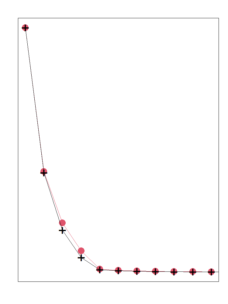
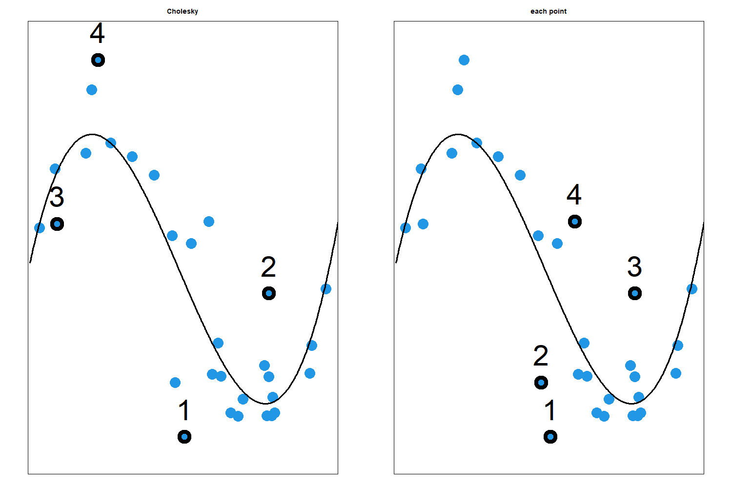
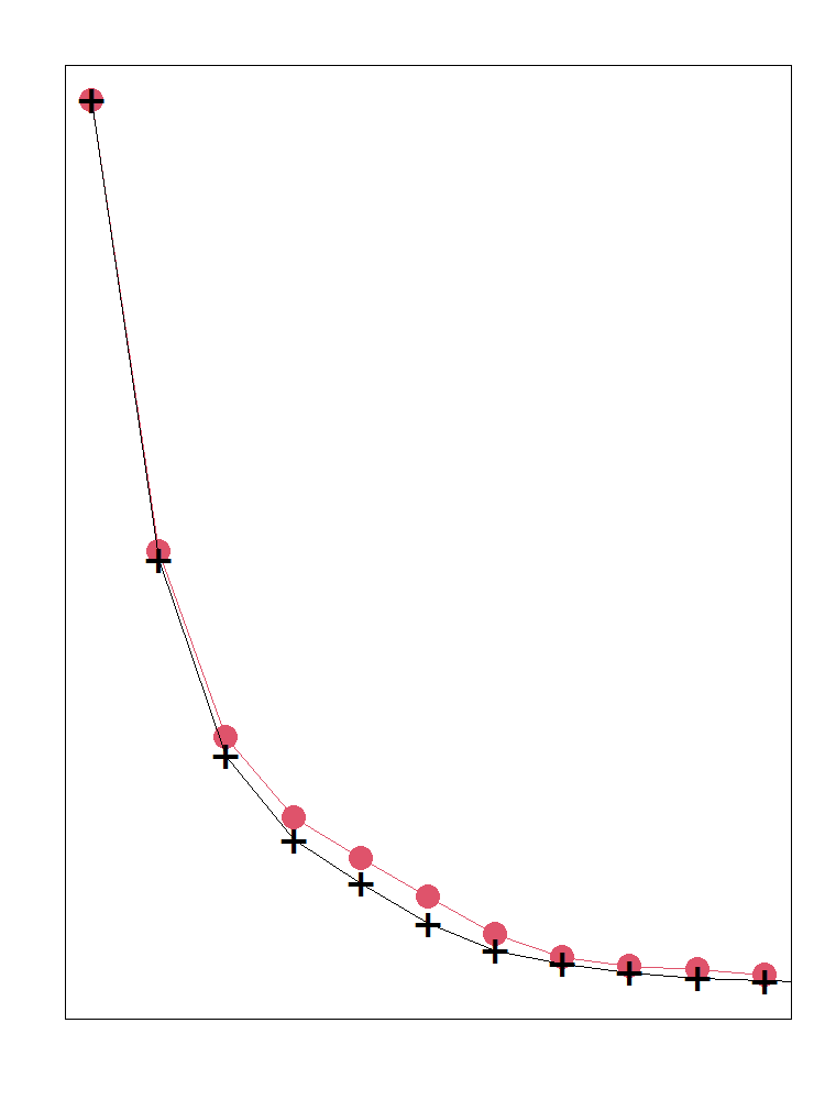
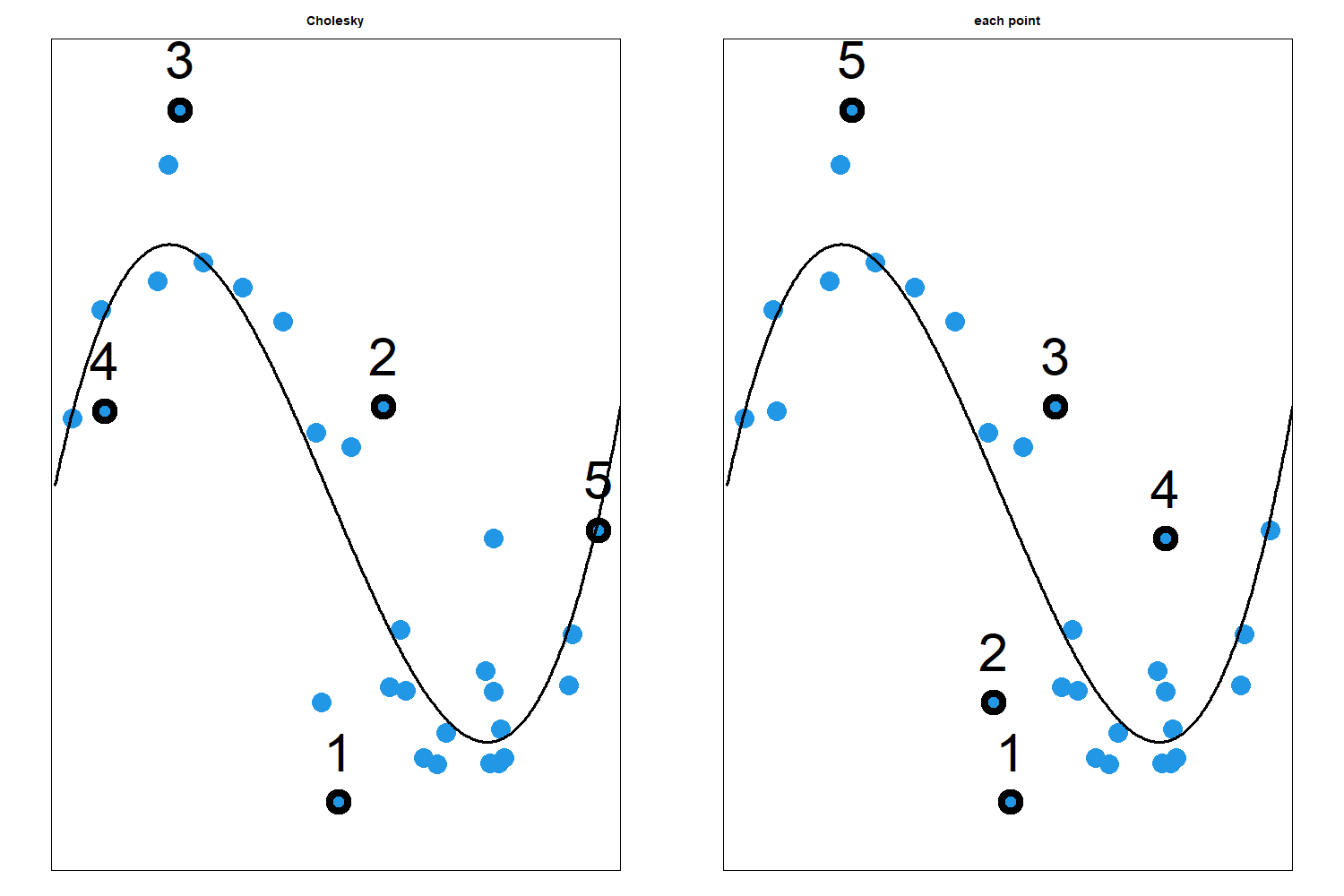
Figure 5. Residual variance and representing sets of the observations. The first and second row of the figure corresponds to the case with a given variance and the estimated variance, respectively. In the leftmost panel of each row, residual variances by incomplete Cholesky decomposition (red dot) and by optimal selection of the subspace (black $+$) are compared; the horizontal axis shows the dimension of the subspace and the vertical axis shows the residual variance. In the middle and right panels of each row, the set of selected points are shown. The middle panel shows points selected by incomplete Cholesky decomposition, while the right panel shows the result of an independent selection. The selected points are encircled and a number above the point shows the order of choice in each algorithm; note that these numbers are not the index $i$ of the observation. The number of selected points shown in the panel is four in the case of a given variance and five in the case of the estimated variance, respectively.

5.2. Dimensional reduction in approximate bootstrap

In this subsection, we explore efficient and accurate implementations of approximate bootstrap algorithms for posterior means; a common feature of these algorithms is to circumvent repeated applications of MCMC to each of the resampled data. First, we implement the first- and second-order approximations based on the Bayesian IJK, as well as an importance sampling approach by Lee et al., (2017); they are compared in an example of fitting the Weibull distribution. Then, we argue that essential subspace can be a useful tool to save computational burden for large sample size $n$.

Approximate bootstrap

Let us assume that a bootstrap replicate $X^{(B)}=(X^{(B)}_{1},X^{(B)}_{2},\ldots,X^{(B)}_{n})$ of the original data $X^{n}=(X^{n}_{1},X^{n}_{2},\ldots,X_{n})$ is generated by the resampling with replacement using random numbers $(R_{1},R_{2},\ldots,R_{n})$ that obey $\mathsf{Multinomial}\left(\frac{1}{n},\frac{1}{n},\ldots,\frac{1}{n}\right).$ Also, we will denote arbitrary statistics of our interest as $A(\theta)$. Then, our task is to approximate the posterior mean $A^{(B)}=\mathbf{E}_{\mathrm{pos}}[A(\theta)\mid X^{(B)}]$ defined with a bootstrap replicate $X^{(B)}$, using only a set $\{\theta^{(m)}\},\,m=,\ldots,M$ of the parameter $\theta$ generated from the posterior with the original data $X^{n}$.

We start from a first-order Bayesian IJK approximation to the bootstrap given in Sec.3.3 of Giordano and Broderick, (2023). This corresponds to the use of terms up to the first-order in $\eta_{i}$s in the right hand side of the formula (10), which provides the following algorithm to compute $A^{(B)}$ for $(R_{1},R_{2},\ldots,R_{n})$

(94) $$A^{(B)}=\mathbf{E}_{\mathrm{pos}}[A]+ \sum_{i=1}^{n}(R_{i}-1)\mathrm{Cov}_{\mathrm{pos}}[A(\theta),\ell(X_{i};\theta)].$$

Also, by using all terms in the right hand side of (10), we obtain a second-order version of (94) as

(95) $$A^{(B)}=\mathbf{E}_{\mathrm{pos}}[A]+ \sum_{i=1}^{n}(R_{i}-1)\,\mathrm{Cov}_{\mathrm{pos}}[A(\theta),\ell(X_{i};\theta)]$$

$$+\frac{1}{2}\sum_{i,j=1}^{n}(R_{i}-1)\,(R_{j}-1)\,{\mathcal{K}_{\mathrm{pos}}}[A(\theta),\ell(X_{i};\theta),\ell(X_{j};\theta)].$$

Before applying these formulae to various sets of $(R_{1},R_{2},\ldots,R_{n})$, we perform a single run of MCMC for the original data $X^{n}$ to obtain posterior samples $\{\theta^{(m)}\},\,m=1,\ldots,M$. These samples are used to estimate $\mathbf{E}_{\mathrm{pos}}[A]$ , $\mathrm{Cov}_{\mathrm{pos}}[A(\theta),\ell(X_{i};\theta)]$, and ${\mathcal{K}_{\mathrm{pos}}}[A,\ell(X_{i};\theta),\ell(X_{j};\theta)]$ in (94) or (95); they are replaced by the estimates calculated as:

(96) $$\widehat{\mathbf{E}}_{\mathrm{pos}}[A]=\frac{1}{M}\sum_{m=1}^{M}{A(\theta^{(m)})},\,\,\,\,\,\,\widehat{\mathbf{E}}_{\mathrm{pos}}[\ell(X_{i};\theta)]=\frac{1}{M}\sum_{m=1}^{M}{\ell(X_{i};\theta^{(m)})},$$

(97) $$\widehat{\mathrm{Cov}}_{\mathrm{pos}}[A(\theta),\ell(X_{i};\theta)]=\frac{1}{M}\sum_{m=1}^{M}\left\{{\left(A(\theta^{(m)})-\widehat{\mathbf{E}}_{\mathrm{pos}}[A]\right)\left(\ell(X_{i};\theta^{(m)})-\widehat{\mathbf{E}}_{\mathrm{pos}}[\ell(X_{i};\theta)]\right)}\right\},$$

(98) $${\widehat{\mathcal{K}}_{\mathrm{pos}}}[A,\ell(X_{i};\theta),\ell(X_{j};\theta)]=$$

(99) $$\,\,\,\frac{1}{M}\sum_{m=1}^{M}\left\{{\left(A(\theta^{(m)})-\widehat{\mathbf{E}}_{\mathrm{pos}}[A]\right)\left(\ell(X_{i};\theta^{(m)})-\widehat{\mathbf{E}}_{\mathrm{pos}}[\ell(X_{i};\theta)]\right)\left(\ell(X_{j};\theta^{(m)})-\widehat{\mathbf{E}}_{\mathrm{pos}}[\ell(X_{j};\theta)]\right)}\right\}.$$

Note that the resultant algorithms only require a single initial run of MCMC with the original data $X^{n}$ and no additional MCMC runs are needed for each realization of $R_{i}$s.

As discussed in Giordano and Broderick, (2023), when we identify the bootstrap covariance between $A^{(B)}$ and $B^{(B)}$ to the frequencist’s covariance, the formula (94) gives a heuristic derivation of the frequencist’s covariance formula (12). On the other hand, if we approximate $(R_{i}-1)$s in (94) with mutually independent normal random variates each of which obeys $N(0,1)$, the same argument leads to the simplified form (13).

Approximate bootstrap and essential subspace

Using (32), the first-order approximate bootstrap (94) can be implemented within an essential subspace as

(100) $$A^{(B)}=\mathbf{E}_{\mathrm{pos}}[A(\theta)]+\sum_{a=1}^{a_{M}}\mathrm{Cov}_{\mathrm{pos}}[A(\theta),\mathcal{L}_{a}(\theta)]\widetilde{\eta}_{a},\,\,\,\widetilde{\eta}_{a}=\sum_{i=1}^{n}U^{i}_{a}(R_{i}-1).$$

This expression is useful to understand the role of the essential subspace in assessing frequencist’s properties. That is, the approximate bootstrap can be implemented only by using projections $(\widetilde{\eta}_{a})$ of the random number $(R_{i})$ to the essential subspace, whose numbers is $a_{M}$ in total. If we approximate $R_{i}$s by IID normal random numbers, and utilized that $\bm{U}=(U^{i}_{a})$ is an orthogonal matrix, $\widetilde{\eta}_{a}$s are further simplified to a set of mutually independent random numbers each of which obeys $N(0,1)$.

On the other hand, the expression (100) is not particularly useful in reducing computational costs, except that we need huge number of bootstrapped estimates in a problem of a small sample size $n$. It is because the eigenvalue problem to compute the essential subspace usually requires more computation than a direct iteration of (94). In the following, we will discuss that the essential subspace will be more useful for the reduction of computational costs in the second-order algorithm based on (95).

Example of the approximate bootstrap

Before discussing issues on dimensional reduction using the essential subspace, we will give an example of the approximate bootstrap. In addition to the first- and second-order algorithm defined by (94) and (95), we also consider an importance sampling (IS) algorithm proposed in Lee et al., (2017), which utilizes the formula

(101) $$A^{(B)}=\sum_{m=1}^{M}A(\theta^{(m)})\mathsf{W}^{(m)},\,\,\,\mathsf{W}^{(m)}=\frac{\prod_{i=1}^{n}\exp((R_{i}-1)\,\ell(X_{i};\theta^{(m)}))}{\sum_{m=1}^{M}\prod_{i=1}^{n}\exp((R_{i}-1)\,\ell(X_{i};\theta^{(m)}))}.$$

As before, $M$ is the number of the posterior samples obtained by an initial MCMC run using the original data $X^{n}$; $A(\theta^{(m)})$ and $\ell(X_{i};\theta^{(m)})$ denote the values of the statistics $A(\theta)$ and the likelihood $\ell(X_{i};\theta)$ computed from the $m$th posterior sample $\theta^{(m)}$. Averaged over the sets $\{\theta^{(m)}\}$ of samples from the original posterior, the right hand side of (101) exactly gives $A^{(B)}$. However, as we will see in the following examples, it often shows a large variance with a finite number $M$ of posterior samples. The formulae (94) and (95) can be regarded as biased but more stable approximations of (101).

As an example, let us consider the Weibull analysis of the life-span data discussed in Sec. 3.4. Target statistics are the following two: (i) The posterior mean $T^{\gamma}(X^{n})=\mathbf{E}_{\mathrm{pos}}[\gamma\mid X^{n}]$ of the shape parameter $\gamma$. (ii) The predictive probability that $X>40$, which is represented as a posterior mean

(102) $$T^{\,>40}(X^{n})=\int_{40}^{\infty}p^{wb}(\widetilde{x}\mid\gamma,\lambda)p(\gamma,\lambda\mid X^{n})d\widetilde{x}=\mathbf{E}_{\mathrm{pos}}\left[\int_{40}^{\infty}p^{wb}(\widetilde{x}\mid\gamma,\lambda)\,d\widetilde{x}\right].$$

Here $p^{wb}(\cdot\mid\gamma,\lambda)$ is the likelihood defined by the density (35) and $p(\gamma,\lambda\mid X^{n})$ is the joint posterior density of $\gamma$ and $\lambda$.

In Fig. 6, the upper set of panels shows the results for $T^{\gamma}(X^{n})$ by blue dots, while lower set of panels shows the results for $T^{\,>40}(X^{n})$ by red dots. In each of the upper and lower set, three panels are shown, which correspond to the first-order approximation (94), the second-order approximation (95), and the importance sampling (IS) estimator (101), respectively. In each panel, the horizontal axis shows the result of the full MCMC computation, while the vertical axis shows the corresponding result of the algorithms based on (94), (95), or (101). Each dot in a panel corresponds to a particular realization of $(R_{1},R_{2},\ldots,R_{n})$. Note that approximations discussed here are applied for each realization of $(R_{1},R_{2},\ldots,R_{n})$. Then, it is reasonable to compare the outputs of the algorithms for each set of $(R_{1},R_{2},\ldots,R_{n})$.

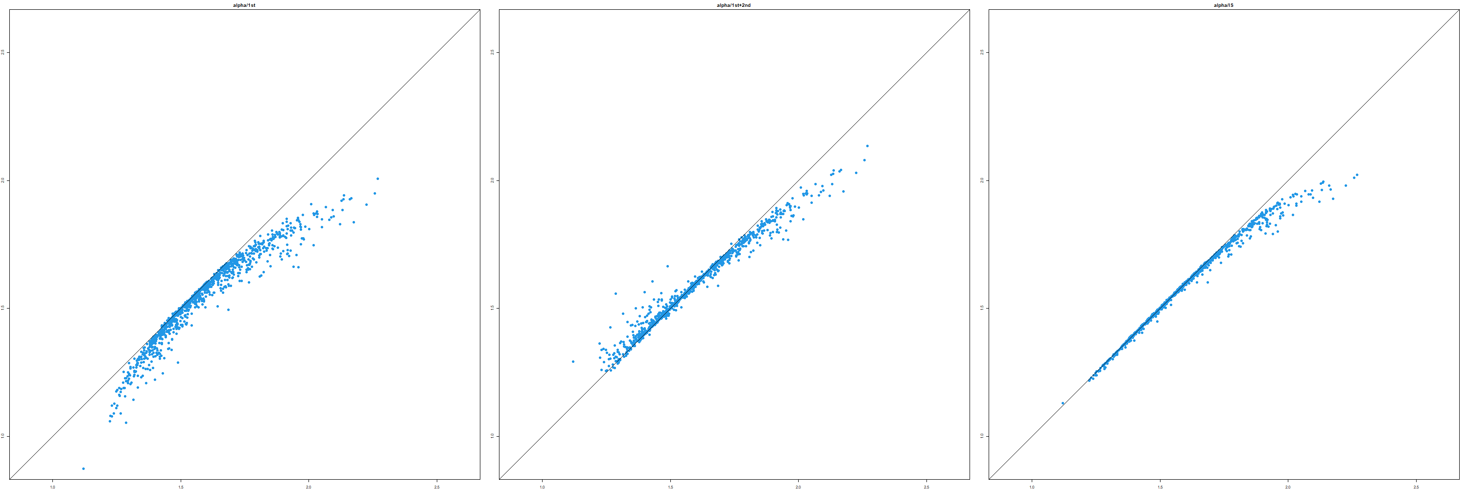
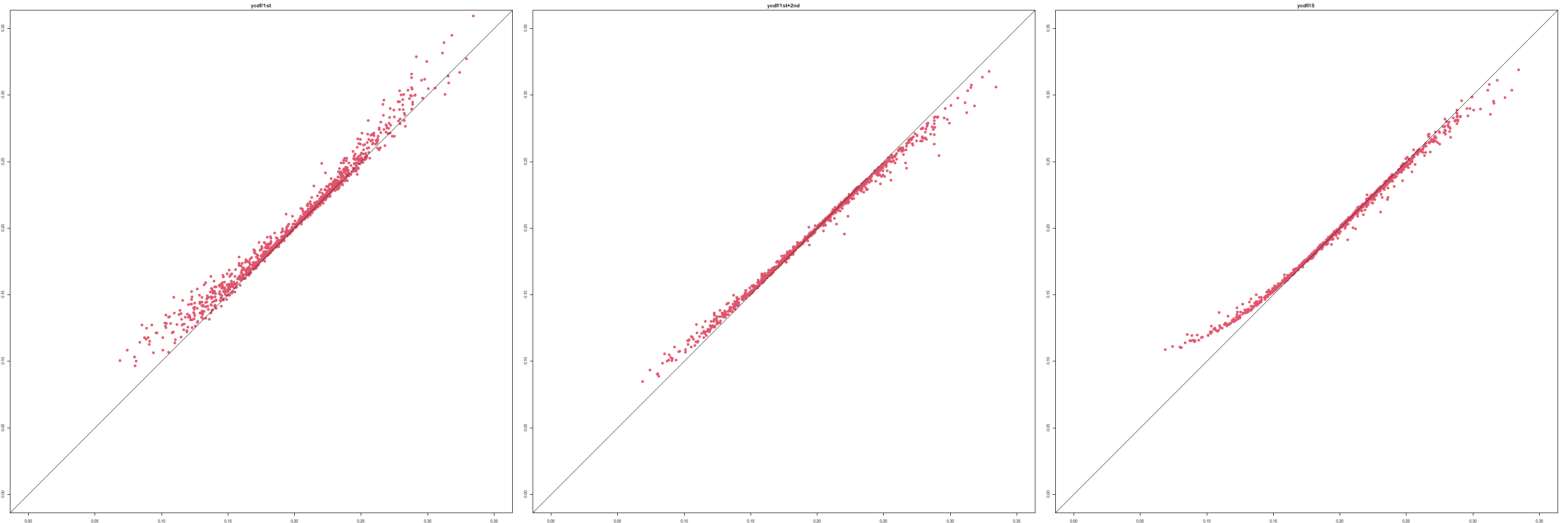
Figure 6. Approximate bootstrap by (94), (95), and (101). Upper three panels show the results for $T^{\gamma}(X^{n})$ by blue dots, while lower three panels show the results for $T^{\,>40}(X^{n})$ by red dots. From the left to the right, results corresponding to (94), (95), and (101) are shown in this order. In each panel, the horizontal axis shows the result of the full MCMC computation, while the vertical axis shows the result of each algorithm for the same realization of $(R_{1},R_{2},\ldots,R_{n})$; the 45 degree guideline is also shown. Each dot in a panel corresponds to a particular realization of $(R_{1},R_{2},\ldots,R_{n})$. The number $N_{b}$ of the realization of $(R_{1},R_{2},\ldots,R_{n})$ is 1000.

The first two columns in Fig. 6 show that the first-order approximation (94) is outperformed by the second-order approximation (95), especially in extremes of the bootstrap distributions. Note, however, that the tails of the distribution may be overemphasised in these plots; usually, most of 1000 points in a plot are in the central part and overlapped together. The importance sampling estimator (101) looks better than the second-order algorithm (95) in the left tail of $T^{\gamma}(X^{n})$, but worse or comparable in other tail regions.

A problem of the importance sampling estimator (101) is that it is sensitive to the choice of the posterior samples generated by the initial MCMC run. This is caused by the non-uniformity of the weights; for some choice of $(R_{1},R_{2},\ldots,R_{n})$, only small number of the weights has a large weight $\mathsf{W}_{i}$, which causes instability of the weighted average and loss of the accuracy of the approximation. A similar problem in importance sampling CV is discussed in Peruggia, (1997). We will see a more severe case of this instability in the next example of this subsection.

Table 1 shows the computational time of these algorithms measured by proc.time () in base R. Note that computational time much depends on the length of the utilized MCMC computations and the size of posterior samples, as well as other implementation details. Also, the elapsed time measured by proc.time () fluctuates depending on the status of computers. Keeping these in our mind, the result in the table 1 indicates that all of the three algorithms of approximate bootstrap is much faster than the naive method that repeats MCMC runs for every realization of $(R_{1},R_{2},\ldots,R_{n})$. In fact, the first-order and second-order algorithms spent most part of the computational time in the initial MCMC run with the original data (about 4 seconds). On the other hand, the importance sampling algorithm (101) is considerably slower compared with other two algorithms even when the number $N_{b}$ of realizations $(R_{1},R_{2},\ldots,R_{n})$ is 1000; it becomes almost nine times larger when $N_{b}$ increases to $10000$. The importance sampling algorithm (101) requires $O(n\times M)$ computation for each realization of $(R_{1},R_{2},\ldots,R_{n})$ and has a disadvantage in computing when $N_{b}$ becomes large.

Algorithm	$N_{b}=1000$	$N_{b}=10000$
repeated MCMC	929	NA
first-order algorithm by eq.(94)	4	5
second-order algorithm by eq.(95)	6	7
importance sampling by eq.(101)	29	259

Table 1. Computational time in seconds for approximate bootstraps in Weibull-fitting. $N_{b}$ indicates the number of the realizations $(R_{1},R_{2},\ldots,R_{n})$. The length of the initial MCMC run for the original data is 30000 in total and the size of the generated samples is 13500. The repeated MCMC, which is only performed when $N_{b}=1000$, utilizes a run of the length 9000 for each set of $(R_{1},R_{2},\ldots,R_{n})$. Time for compiling stan codes is not included.

Dimensional reduction using the essential subspace

As remarked in the previous example, the importance sampling algorithm (101) requires $O(n\times M\times N_{b})$ computation for $N_{b}$ realization of $(R_{1},R_{2},\ldots,R_{n})$ and has a disadvantage when a large number $N_{b}$ of bootstrap replications is required.

On the other hand, a disadvantage of the second-order algorithm (95) is that treating $n\times n$ matrix ${\mathcal{K}_{\mathrm{pos}}}[A,\ell(X_{i};\theta),\ell(X_{j};\theta)]$ requires $O(n^{2}\times N_{b})$ computational time. The construction of this matrix also required $O(n^{2}\times M)$ computation to initialize the algorithm, where $M$ is the number of the posterior samples. The $n^{2}$ dependence on the sample size $n$ may cause a serious increase of the computational burden, when the sample size becomes large.

In fact, it is easy to implement the second-order approximation (95) with the computational requirement $O(n\times M\times N_{b})$. If we define $\mathsf{L}(\theta;(R_{i}))=\sum_{i=1}^{n}(R_{i}-1)\ell(X_{i};\theta)$, the second-order term

(103) $$\sum_{i,j=1}^{n}(R_{i}-1)(R_{j}-1)\,{\mathcal{K}_{\mathrm{pos}}}[A,\ell(X_{i};\theta),\ell(X_{j};\theta)],$$

in the right hand side of (95) is expressed as

(104) $${\mathcal{K}_{\mathrm{pos}}}\left[A(\theta),\mathsf{L}(\theta;(R_{i})),\mathsf{L}(\theta;(R_{j}))\right].$$

Once we fix the random number $R_{i}$s, the computation of $\mathsf{L}(\theta^{(m)};(R_{i}))$ for $\theta^{(m)},\,m=1,\ldots,M$, requires $O(n\times M)$ computation. Using them, it requires only $O(1)$ computation to obtain the empirical estimate of (104). Hence the total computational time is in the order of $O(n\times M\times N_{b})$. This implementation will be a practical choice when $n$ is large, but it can be ineffective when the number $N_{b}$ of the bootstrap replications also becomes large. A possible remedy is to reduce the number $M$ of MCMC samples, but the effect to the accuracy of the approximation is yet to be studied.

Alternatively, we propose here to approximate the second-order term (103) using the projections to the essential subspace. This gives

(105) $$\sum_{\alpha,\beta=1}^{a_{M}}\widetilde{\eta}_{\alpha}\,\widetilde{\eta}_{\beta}\,{\mathcal{K}_{\mathrm{pos}}}[A,\mathcal{L}_{\alpha}(\theta),\mathcal{L}_{\beta}(\theta)],\,\,\,\mathcal{L}_{\alpha}(\theta)=\sum_{i=1}^{n}U^{i}_{a}\ell(X_{i};\theta),\,\,\,\widetilde{\eta}_{a}=\sum_{i=1}^{n}U^{i}_{a}(R_{i}-1).$$

as an approximation to (103). If we adopt this approximation and use the incomplete Cholesky decomposition, an extra computation of the order $O(a_{M}^{2}\times n)$ is required to initialize the algorithm, where $a_{M}$ is the dimension of the essential subspace. On the other hand, the computational time to construct the empirical version of the matrix ${\mathcal{K}_{\mathrm{pos}}}$ reduces to $O(a_{M}^{2}\times M)$; also the time to approximate $N_{b}$ bootstrap replications reduces to $O(a_{M}\times n\times N_{b})$.

The rest of the problem is the construction of $n\times n$ matrix $W$ using posterior samples; this still requires $O(n^{2}\times M)$ computation. In the following example, we utilized a posterior sub-sampling approach to circumvent this difficulty. That is, using the smaller number $M^{*}$ of posterior samples, the matrix $W$ is constructed and a rough approximation of the essential subspace is obtained using the incomplete Cholesky decomposition. Then, using the projections $\mathcal{L}_{\alpha}(\theta),\,\alpha=1,\ldots,a_{M}$ to this approximate subspace, we construct ${\mathcal{K}_{\mathrm{pos}}}[A,\mathcal{L}_{\alpha}(\theta),\mathcal{L}_{\beta}(\theta)]$ using the full set of posterior samples. By using this approach, the amount of the computation to initialize the algorithm can reduce to $O(n^{2}\times M^{*})$.

The posterior sub-sampling approach is not perfect, because we should still store a $n\times n$ matrix in the memory, which becomes difficult for a very large sample size $n$. A promising way to deal with this problem is the use of on-line PCA (Oja, (1992); Cardot and Degras, (2017)) to compute the essential subspace, which is the subject of our ongoing study.

Example of the dimensional reduction

Here we consider the state space model for the Prussian horse data discussed in Sec. 3.4 as an example of the proposed algorithm. The states $(Z_{t})$ are regarded as fixed but unknown variables and the likelihoods conditioned on $(Z_{t})$ is considered. At each time $t,\,t=1,\ldots,20$, there are 14 observations, each of which corresponds to one of the 14 coups in Prussian. Bootstrap replication is defined as sampling with replacement from the set of 14 observations at each time. Target statistics are the posterior mean $\mathbf{E}_{\mathrm{pos}}[\exp(Z_{t})]$ of the intensity of the Poisson distribution at each time $t$. Note that this is a rather unfavorable condition both for the bootstrap and the proposed approximations, since they are based on a large sample theory.

The first-order algorithm (94), the original second-order algorithm (95), second-order algorithms with the projection to the subspace $a_{M}=20$ and $a_{M}=8$, and the estimate using importance sampling (101) are compared to the result of the repeated applications of MCMC. The first-order term in (95) is always directly computed and projection to subspace is not used. Note that even the dimension $a_{M}=20$ of the subspace is much smaller than $n=20\times 14=280$. In the last two algorithms, the size $M^{*}$ of the subset of posterior samples to construct the essential subspace is set to 100, while the total number $M$ of posterior samples is 4500.

First, let us see the computational time given in the table 2; it is again measured by proc.time () in base R and fluctuates considerably depending on the status of the computer. As expected, the naive method using repeated MCMC requires huge computational time. Also, the original second-order algorithm based on (95) is significantly slower that other algorithms. Most of the computational time (169 seconds) spent on the construction of the matrix ${\widehat{\mathcal{K}}_{\mathrm{pos}}}$ whose size is $20\times 280\times 280$ using 4500 posterior samples. Also, the computation of (95) for each set of $(R_{1},R_{2},\ldots,R_{n})$ requires considerable computational time (23 seconds in total). The importance sampling algorithm (101) again becomes slow when $N_{b}=10000$. On the other hand, the first-order and second-order algorithms that utilize the essential subspace approximations perform almost equally well in computational time. The initial MCMC requires about 29 seconds, which consists of the most part of computational time required for these algorithms. Note that we use the same matrix $W$ to estimate all $20$ parameters; hence even when the size $M^{*}$ of the set to construct the matrix $W$ changes from $100$ to $4500$, the increase of computational time is within a few seconds.

Algorithm		$N_{b}=1000$	$N_{b}=10000$
repeated MCMC		12101	NA
first-order algorithm by eq.(94)		30	39
second-order algorithm by eq.(95)		222	433
essential subspace ($a_{M}=8\>\>$, $M^{*}=100$)		31	42
essential subspace ($a_{M}=20$, $M^{*}=100$)		32	45
essential subspace ($a_{M}=8\>\>$, $M^{*}=4500$)	$\dagger$	34	47
essential subspace ($a_{M}=20$, $M^{*}=4500$)	$\dagger$	35	50
importance sampling by eq.(101)		47	208

Table 2. Computational time in seconds for approximate bootstraps in the state space model. Here “essential subspace” means the second-order algorithm utilizing a projection to a subspace of dimension $a_{M}$. Entries marked by $\dagger$ are not included in Fig. 7. The length of the initial MCMC run for the original data is 12000 in total and the size of the generated samples is 4500. The repeated MCMC, which is only performed when $N_{b}=1000$, utilizes a run of the length 4000 for each set of $(R_{1},R_{2},\ldots,R_{n})$. Time for compiling stan codes is not included. The elapsed time measured by proc.time () fluctuates considerably depending on the system status, which makes the significant digits at most two.

Next, we discuss the accuracy of the results shown in Fig. 7. As before, in each panel, the horizontal axis shows the result of the repeated MCMC computation, while the vertical axis shows the result of approximate algorithms. Each of the points in the panel corresponds to a particular realization of $(R_{1},R_{2},\ldots,R_{n})$. The rows corresponds to the time $t$; to save the space, only the results of $t=1,6,11,16$ are shown.

The first and second columns show the results of the first-order algorithm (94) and the original second-order algorithm (95); the difference is not large, but the second-order algorithm seems to perform better. The third and fourth columns show the results of the second-order algorithm using the projection to a subspace. The fourth column, where $a_{M}=20$ may be enough to cover the essential subspace, provides a good approximation to the original second-order algorithm. On the other hand, the third column, where $a_{M}=8$, point by point agreement to the original second-order algorithm becomes much worse. However, the overall tendency of the approximation is similar to the original second-order algorithm given in the second column.

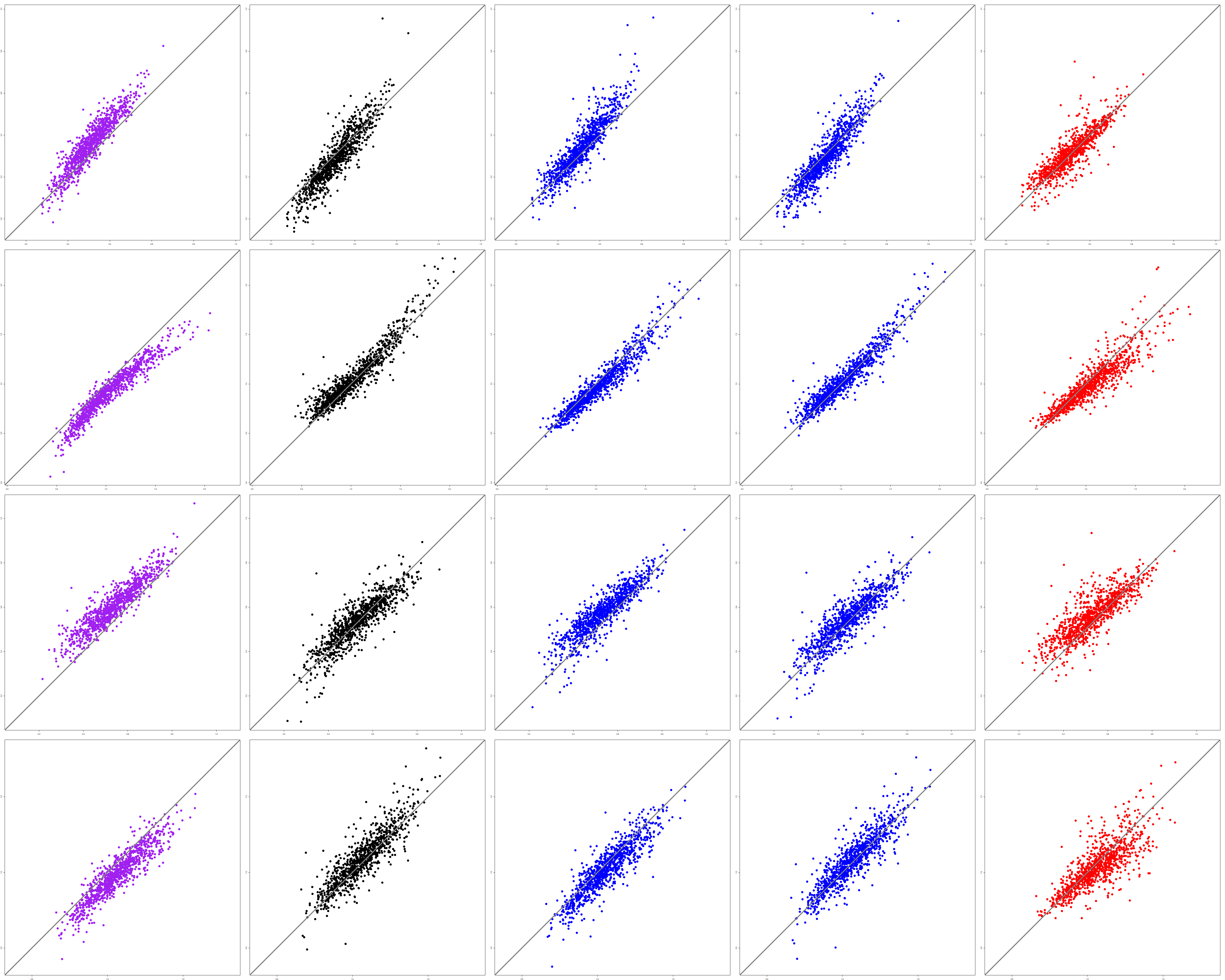
Figure 7. Dimensional reduction in approximate bootstrap. From the top to the bottom, each row corresponds to $i=1,6,11,16$, respectively. From the left to the right, the results of the first-order algorithm (94) (violet), the original second-order algorithm (95) (black), second-order algorithms using projections to essential subspaces with $a_{M}=8$ and $a_{M}=20$ (both in blue), importance sampling (101) (red) are shown. In each panel, the horizontal axis shows the result of repeated MCMC computation, while the vertical axis shows the result of approximate algorithms for the same set of $(R_{1},R_{2},\ldots,R_{n})$; the 45 degree guideline is also shown. Each dot in a panel corresponds to a particular realization of $(R_{1},R_{2},\ldots,R_{n})$. The number of the realization of $(R_{1},R_{2},\ldots,R_{n})$ is 1000.

Finally, the fifth column gives estimates by the importance sampling (101), which shows a considerably divergent behavior. The erratic nature of estimates is explained by the extreme concentration of weights into small number of posterior samples in some realizations of $(R_{1},R_{2},\ldots,R_{n})$. To see this, the values of weights $\mathsf{W}_{i}$ are plotted in Fig. 8 for 200 sets of $(R_{1},R_{2},\ldots,R_{n})$. The maximum value of the weights exceeds 0.4 for considerable number of realizations $(R_{1},R_{2},\ldots,R_{n})$; in some cases, it even surpasses 0.7 or 0.8. Since the sum of the weights is normalized to the unity within each set, $\mathsf{W}_{i}=0.4$ ($0.7$) means that 40% (70%) of the weight is concentrated on a single sample among 4500 posterior samples.

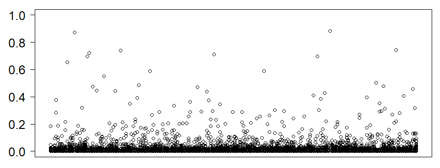
Figure 8. Relative size of weights $\mathsf{W}_{i}$ in the state space model for 200 sets of $(R_{1},R_{2},\ldots,R_{n})$. The horizontal axis corresponds to the indices $1,\cdots,200$ of the set and the vertical axis shows the values of the weights. For each set of $(R_{1},R_{2},\ldots,R_{n})$, the sum of the weights is normalized to the unity. The function boxplot () in base R graphics is used; the points in the figure are outliers detected by boxplot() and boxes are almost hidden in the bottom of the figure.

6. Summary and future problems

The scope of this study is to provide a unified view on a variety of seemingly unrelated fields along the axis of the matrix $W$, which is defined as a covariance matrix between log-likelihood of each observation. We utilize the idea of the Bayesian infinitesimal jackknife (Giordano and Broderick, (2023)) to connect the posterior covariance and cumulants with the frequencist’s properties.

At the beginning of the paper, we discussed that the posterior covariance matrix $W$ and its eigenvalue problem are relevant in various statistical settings, including the evaluation of the posterior sensitivity, assessment of the frequencist’s uncertainty from posterior samples, as well as stochastic expansions of the loss discussed in the appendix C. We named the principal space of the matrix $W$ as an essential subspace. Following that, a kernel formulation of the problem is presented. Here the matrix $W$ is interpreted as a reproducing kernel, which we termed as W-kernel. The proposed framework elucidated a connection to existing studies on natural kernels, such as the Fisher kernel and neural tangent kernel; it also revealed duality relations with the W-kernel. The role of informative priors is also discussed in relation to the centering in frequencist’s covariance formulae. We also discussed two examples of applications. The first one is the selection of a representative set of observations, where incomplete Cholesky decomposition is efficiently used. Another example is to construct an efficient approximate bootstrap algorithm for Bayesian estimators, where a projection to the essential subspace is shown to be useful.

There are a number of problems left for future studies: The use of incomplete Cholesky decomposition reduces the computational burden to obtain an essential subspace, but we should still compute a $n\times n$ matrix and store it in a memory. As discussed in the last section, the use of on-line PCA (Oja, (1992); Cardot and Degras, (2017)) to compute the essential subspace can be useful to circumvent this difficulty. Some part of this paper may be generalize to singular models in the sense of Watanabe, (2018), or even useful in high-dimensional settings (Okuno and Yano, (2023); Giordano and Broderick, (2023)); researches in these directions are also relevant, as well as to provide mathematically rigorous proofs of the results intuitively derived in this paper.

Appendix A Derivation of Formulae

A.1. Approximation (16) of the KL-divergence

Let us consider the KL-divergence between the original and weighted posterior defined by

(106) $$D(p(\theta;X^{n})\|p_{w}(\theta;X^{n}))=\mathbf{E}_{\mathrm{pos}}\left[\log\frac{p(\theta;X^{n})}{p_{w}(\theta;X^{n})}\right],$$

where $p_{w}$ is given by the equation (5). When we are interested in derivatives with respect to $w_{i}$ or $\eta_{i}=w_{i}-1$, the right hand side of (106) can be replaced by

(107) $$\mathbf{E}_{\mathrm{pos}}[-\log p_{w}(\theta;X^{n})].$$

Hereafter, we again assume regularity conditions that allow the exchange of derivatives and integrals.

First, we calculate the first-order log-derivatives of the weighted posterior (5) as

(108) $$\frac{\partial}{\partial w_{i}}\log p_{w}(\theta;X^{n}) =\ell(X_{i};\theta)-\frac{\partial}{\partial w_{i}}\left[\log\textstyle\int\exp\left\{\sum_{m=1}^{n}w_{m}\,\ell(X_{m};\theta)\right\}p(\theta)d\theta\right]$$

(109) $$=\ell(X_{i};\theta)-\frac{\textstyle\int\ell(X_{i};\theta)\exp\left\{\sum_{m=1}^{n}w_{m}\,\ell(X_{m};\theta)\right\}p(\theta)d\theta}{\textstyle\int\exp\left\{\sum_{m=1}^{n}w_{m}\,\ell(X_{m};\theta)\right\}p(\theta)d\theta}$$

(110) $$=\ell(X_{i};\theta)-\mathbf{E}_{\mathrm{pos}}^{w}[\ell(X_{i};\theta)].$$

Also, from the definition of the weighted posterior (5) and the weighted posterior mean (6), a direct calculation of the derivative gives

(111) $$\frac{\partial}{\partial w_{j}} \mathbf{E}_{\mathrm{pos}}^{w}[A(\theta)]=\frac{\partial}{\partial w_{j}}\left[\frac{\textstyle\int A(\theta)\exp\left\{\sum_{m=1}^{n}w_{m}\,\ell(X_{m};\theta)\right\}p(\theta)d\theta}{\textstyle\int\exp\left\{\sum_{m=1}^{n}w_{m}\,\ell(X_{m};\theta)\right\}p(\theta)d\theta}\right]$$

(112) $$\qquad= \frac{\textstyle\int A(\theta)\ell(X_{j};\theta)\exp\left\{\sum_{m=1}^{n}w_{m}\,\ell(X_{m};\theta)\right\}p(\theta)d\theta}{\textstyle\int\exp\left\{\sum_{m=1}^{n}w_{m}\,\ell(X_{m};\theta)\right\}p(\theta)d\theta}$$

(113) $$-\frac{\textstyle\left[\int A(\theta)\exp\left\{\sum_{m=1}^{n}w_{m}\,\ell(X_{m};\theta)\right\}p(\theta)d\theta\right]\textstyle\left[\int\ell(X_{j};\theta)\exp\left\{\sum_{m=1}^{n}w_{m}\,\ell(X_{m};\theta)\right\}p(\theta)d\theta\right]}{\left[\textstyle\int\exp\left\{\sum_{m=1}^{n}w_{m}\,\ell(X_{m};\theta)\right\}p(\theta)d\theta\right]^{2}}$$

(114) $$=\, \mathbf{E}_{\mathrm{pos}}^{w}[A(\theta)\,\ell(X_{j};\theta)]\,-\,\mathbf{E}_{\mathrm{pos}}^{w}[A(\theta)]\,\mathbf{E}_{\mathrm{pos}}^{w}[\ell(X_{j};\theta)]$$

From (108), using (111) with $A(\theta)=\ell(X_{i};\theta)$, we have

(115) $$\frac{\partial^{2}}{\partial w_{i}\partial w_{j}}\log p_{w}(\theta;X^{n}) =\frac{\partial}{\partial w_{j}}\left[\ell(X_{i};\theta)-\mathbf{E}_{\mathrm{pos}}^{w}[\ell(X_{i};\theta)]\right]$$

(116) $$=-\big{\{}\,\mathbf{E}_{\mathrm{pos}}^{w}[\ell(X_{i};\theta)\ell(X_{j};\theta)]\,-\,\mathbf{E}_{\mathrm{pos}}^{w}[\ell(X_{i};\theta)]\mathbf{E}_{\mathrm{pos}}^{w}[\ell(X_{j};\theta)]\,\big{\}}.$$

Then, from (108) and (115), the exchange of the derivatives and $\mathbf{E}_{\mathrm{pos}}^{w}$ gives

(117) $$\qquad\frac{\partial}{\partial w_{i}}\mathbf{E}_{\mathrm{pos}}^{w}\left[-\log p_{w}(\theta;X^{n})\right] =-\mathbf{E}_{\mathrm{pos}}^{w}[\ell(X_{i};\theta)]+\mathbf{E}_{\mathrm{pos}}^{w}[\ell(X_{i};\theta)]=0,$$

(118) $$\qquad\frac{\partial}{\partial w_{i}\partial w_{j}}\mathbf{E}_{\mathrm{pos}}^{w}\left[-\log p_{w}(\theta;X^{n})\right] =\mathbf{E}_{\mathrm{pos}}^{w}[\ell(X_{i};\theta)\ell(X_{j};\theta)]\,-\,\mathbf{E}_{\mathrm{pos}}^{w}[\ell(X_{i};\theta)]\mathbf{E}_{\mathrm{pos}}^{w}[\ell(X_{j};\theta)].$$

Use $w_{i}=1+\eta_{i}$ to change variables of the derivatives and set $w_{i}=1$ after that, (117) and (118) gives

(119) $$\left.\frac{\partial}{\partial\eta_{i}}D(p(\theta;X^{n})\|p_{w}(\theta;X^{n}))\right|_{w=1} =0,$$

(120) $$\left.\frac{\partial}{\partial\eta_{i}\partial\eta_{j}}D(p(\theta;X^{n})\|p_{w}(\theta;X^{n}))\right|_{w=1} =\mathrm{Cov}_{\mathrm{pos}}[\ell(X_{i};\theta),\ell(X_{j};\theta)].$$

Using (119) and (120) as derivatives of the KL divergence (106), the desired formula (16) is obtained as a second-order Taylor approximation of (106).

A.2. Bounds (26) of the residual variance

Using the relation (22), we have

(121) $$\mathrm{Var}_{\mathrm{pos}}[\ell(X_{i};\theta)-\ell^{*}(X_{i};\theta)]=\mathrm{Var}_{\mathrm{pos}}\left[\sum_{a=a_{M}+1}^{n}U^{a}_{i}\mathcal{L}_{a}(\theta)\right]=\sum_{a=a_{M}+1}^{n}\lambda_{a}|U^{a}_{i}|^{2},$$

On the other hand, since $U=(U^{i}_{a})$ is an orthogonal matrix

(122) $$|U^{a}_{i}|^{2}\leq\sum_{b=1}^{n}|U^{b}_{i}|^{2}=1,$$

which results in

(123) $$\sum_{a=a_{M}+1}^{n}\lambda_{a}|U^{a}_{i}|^{2}\leq\sum_{a=a_{M}+1}^{n}\lambda_{a}.$$

Using (121) and (123), we have a bound of the residuals as

(124) $$\mathrm{Var}_{\mathrm{pos}}[\ell(X_{i};\theta)-\ell^{*}(X_{i};\theta)]\leq\sum_{a=a_{M}+1}^{n}\lambda_{a}.$$

A.3. Feature space representation (71) and its dual (72)

Derivation of the equation (71) and (66)

From (60) and the definition (65) of the principal square root, we can write

(125) $$\,\,\,\frac{1}{n}K_{MF}(X_{i},X_{j}) =\frac{1}{n}\sum_{\gamma=1}^{k}\Biggl{\{}\sum_{\alpha=1}^{k}(\hat{\mathcal{J}}^{-1/2})_{\gamma\alpha}\frac{\partial}{\partial\theta_{\alpha}}\ell(X_{i};\theta)\bigg{|}_{\theta=\hat{\theta}}\Biggr{\}}\Biggl{\{}\sum_{\beta=1}^{k}(\hat{\mathcal{J}}^{-1/2})_{\gamma\beta}\frac{\partial}{\partial\theta_{\beta}}\ell(X_{j};\theta)\bigg{|}_{\theta=\hat{\theta}}\Biggr{\}}$$

(126) $$=\frac{1}{n}\sum_{\gamma=1}^{k}\Phi^{MF}(\gamma,X_{i})\Phi^{MF}(\gamma,X_{j}),$$

which shows (71). It also shows that the first equation of (66) gives a feature vector corresponding to the empirical version of the modified Fisher kernel. A similar calculation from (61) yields $K^{0}_{MF}(X_{i},X_{j})=\sum_{\gamma=1}^{k}\Phi^{MF}_{0}(\gamma,X_{i})\Phi^{MF}_{0}(\gamma,X_{j}),$ and shows the second equation of (66) gives a feature vector corresponding to the population version of the modified Fisher kernel.

Derivation of the equation (72)

From (66), a direct calculation gives

(127) $$\frac{1}{n}\sum_{i=1}^{n}\Phi^{MF}(\gamma,X_{i})\Phi^{MF}(\delta,X_{i})=\frac{1}{n}\sum_{i=1}^{n}\Biggl{\{}\sum_{\alpha=1}^{k}(\hat{\mathcal{J}}^{-1/2})_{\gamma\alpha}\frac{\partial}{\partial\theta_{\alpha}}\ell(X_{i};\theta)\bigg{|}_{\theta=\hat{\theta}}\Biggr{\}}\Biggl{\{}\sum_{\beta=1}^{k}(\hat{\mathcal{J}}^{-1/2})_{\delta\beta}\frac{\partial}{\partial\theta_{\beta}}\ell(X_{i};\theta)\bigg{|}_{\theta=\hat{\theta}}\Biggr{\}}$$

(128) $$=\sum_{\alpha,\beta=1}^{k}(\hat{\mathcal{J}}^{-1/2})_{\gamma\alpha}\,\left[\frac{1}{n}\sum_{i=1}^{n}\left\{\frac{\partial}{\partial\theta_{\alpha}}\ell(X_{i};\theta)\bigg{|}_{\theta=\hat{\theta}}\frac{\partial}{\partial\theta_{\beta}}\ell(X_{i};\theta)\bigg{|}_{\theta=\hat{\theta}}\right\}\right]\,(\hat{\mathcal{J}}^{-1/2})_{\beta\delta}$$

(129) $$=\sum_{\alpha,\beta=1}^{k}(\hat{\mathcal{J}}^{-1/2})_{\gamma\alpha}\,\hat{\mathcal{I}}_{\alpha\beta}(\hat{\mathcal{J}}^{-1/2})_{\beta\delta}=\left(\hat{\mathcal{J}}^{-1/2}\hat{\mathcal{I}}\hat{\mathcal{J}}^{-1/2}\right)_{\gamma\delta},$$

which shows (72).

A.4. Derivation of (81) and (85)

Here, we give a rough sketch of the derivation of the relation (81) for $O(1)$ priors and its generalization (85) for $O(n)$ priors, both of which hold in a regular model.

First, we discuss (81) for $O(1)$ priors. Let us define

(130) $$l_{pos}(\theta)=\frac{1}{n}\sum_{i=1}^{n}\ell(X_{i};\theta)$$

Using the Cauchy-Schwartz inequality, we obtain

(131) $$\mathrm{Cov}_{\mathrm{pos}}\left[A(\theta),nl_{pos}(\theta)\right]\,\leq\,n\bigg{(}\mathrm{Var}_{\mathrm{pos}}\left[A(\theta)\right]\bigg{)}^{1/2}\bigg{(}\mathrm{Var}_{\mathrm{pos}}\left[l_{pos}(\theta)\right]\bigg{)}^{1/2}$$

This shows that it is enough to estimate the order of the variances in the right-hand side.

Then, we expand $A(\theta)$ and $l_{pos}(\theta)$ around the MLE $\hat{\theta}$ defined by $l^{\prime}_{pos}(\theta)=0$ as

(132) $$A(\theta) =A^{\prime}(\hat{\theta})(\theta-\hat{\theta})+o(\|\theta-\hat{\theta}\|),$$

(133) $$l_{pos}(\theta) =\frac{1}{2}(\theta-\hat{\theta})^{T}\,l^{\prime\prime}_{pos}(\hat{\theta})\,(\theta-\hat{\theta})+o(\|\theta-\hat{\theta}\|^{2}),$$

where $A^{\prime}$ and $l^{\prime\prime}_{pos}$ means the matrices of the first and second derivatives and $\|\,\,\,\,\|$ denotes the $\ell_{2}$-norm. Note that $l^{\prime}_{pos}(\hat{\theta})=0$ by the definition of the MLE. They lead to the estimates of the order of the variances as

$$\mathrm{Var}_{\mathrm{pos}}\left[A(\theta)\right] =O_{p}(\mathbf{E}_{\mathrm{pos}}[(\theta-\hat{\theta})^{2}])=O_{p}(1/n),$$

$$\mathrm{Var}_{\mathrm{pos}}\left[l_{pos}(\theta)\right] =O_{p}(\mathbf{E}_{\mathrm{pos}}[(\theta-\hat{\theta})^{4}])=O_{p}(1/n^{2}),$$

where the behavior of $\mathrm{Var}_{\mathrm{pos}}\left[l_{pos}(\theta)\right]$ is crucial for the result. Using them and (131), we obtain

$$\mathrm{Cov}_{\mathrm{pos}} \left[A(\theta),nl_{pos}(\theta)\right]\leq O_{p}(1/\sqrt{n}).$$

This leads to the relation (81):

$$\mathrm{Cov}_{\mathrm{pos}}\left[A(\theta),\sum_{i=1}^{n}\ell(X_{i};\theta)\right]=\mathrm{Cov}_{\mathrm{pos}}\left[A(\theta),nl_{pos}(\theta)\right]=o_{p}(1).$$

Next, we discuss (85) for $O(n)$ priors. For $O(n)$ priors, the expansion (133) no longer holds. However, if we define

(134) $$l^{*}_{pos}(\theta)=\frac{1}{n}\sum_{i=1}^{n}\left\{\ell(X_{i};\theta)+\frac{1}{n}\log p(\theta)\right\}=\frac{1}{n}\sum_{i=1}^{n}\{\ell(X_{i};\theta)+\Lambda\log\widetilde{p}(\theta)\}+o(1/n).$$

and make $\theta^{*}$ a MAP estimate that satisfies $(l^{*}_{pos})^{\prime}(\theta^{*})=0$, we can proceed in the same way, which gives the relation (85):

$$\mathrm{Cov}_{\mathrm{pos}}\left[A(\theta),\sum_{i=1}^{n}\left\{\ell(X_{i};\theta)+\frac{1}{n}\log p(\theta)\right\}\right]=\mathrm{Cov}_{\mathrm{pos}}\left[A(\theta),nl_{pos}(\theta)\right]=o_{p}(1).$$

Appendix B $O(n)$ priors

This section provides supplementary materials on the $O(n)$ priors introduced in the main text. First, we give a simple numerical example that showcase the effect of informative priors to the frequencist’s covariance formulae (12) and (13).

Then, we discuss heuristic derivations of the following properties mentioned in the main text, which hold in the setting of $O(n)$ priors; we will proceed in the order (a) $\Rightarrow$ (c) $\Rightarrow$ (b).

• The original formula (12) with centering gives an asymptotically correct estimate of the frequencist’s covariance even in the $O(n)$ setting.

• The simplified formula (13) without centering does not give an asymptotically correct estimate of the frequencist’s covariance in the $O(n)$ setting.

• The difference between (12) and (13) is $O_{p}(\Lambda^{2})$ when we ignore $o_{p}(1/n)$ terms; it is different from $O_{p}(\Lambda)$ that we naively expect.

Here, we do not intend to give mathematically rigorous proofs, but our arguments will be useful to clarify the difference between the $O(1)$ and $O(n)$ settings on priors.

Finally, we turn to the subject of model selection in the case of $O(n)$ priors; it is shown that the bias correction term of waic is robust against even moderately informative priors. This is an analog of the property (c) in the case of frequencist’s covariance formulae.

B.1. Example of the binomial model with informative priors

First, we consider an example of the binomial model with possibly over-dispersed data. A Bayesian model defined by the binomial likelihood and beta prior are assumed as:

(135) $$X_{i}\sim Binom(N,q),\,\,\,q\sim Beta(\alpha,\beta).$$

In the following experiments, we assume that IID observations $X^{n}=(X_{1},X_{2},\ldots,X_{n})$ are sampled from a beta binomial distribution, whose pmf is:

(136) $$p(x;q_{0},\rho)={}_{N}C_{x}\frac{B(x+\mathrm{a},N-x+\mathrm{b})}{B(\mathrm{a},\mathrm{b})},\,\,\,\mathrm{a}=q_{0}\frac{1-\rho}{\rho},\,\,\,\mathrm{b}=(1-q_{0})\frac{1-\rho}{\rho}.$$

Note that $\mathbf{E}_{X}[X]/N=q_{0}$ when $X\sim p(x;q_{0},\rho)$. The total number of the trials is $nN$.

Below, we will focus on the frequencist’s variance of the posterior mean $\mathbf{E}_{\mathrm{pos}}[q]$, and compare three types of the estimator: (i) The posterior variance $\mathrm{Var}_{\mathrm{pos}}[q]$, (ii) $\hat{\Sigma}_{qq}$ defined by (13), and (iii) $\hat{\Sigma}^{*}_{qq}$ defined by (12). While (i) is a genuine Bayesian estimator, (ii) and (iii) are frequencist’s estimators obtained by the Bayesian IJK. These values are calculated by MCMC for each of the artificial data. On the other hand, the true value of the frequencist’s variance is estimated from $\mathbf{E}_{\mathrm{pos}}[q]$ for the same set of artificial data.

In all experiments here, the number $N$ of the trials in each observation is set to $5$, while the number $n$ of the observations in each set of data is $20$; hence total number of trials in a set of data is $nN=100$. $q_{0}$ is 0.25. The number of the set of artificial data used to construct a boxplot is $800$.

Fig. 9 shows the result of an experiment performed in the $\rho=0$ case, where the model can correctly represent the true distribution. We perform the experiments with the beta prior of $(\alpha,\beta)=(5,1),(10,1),(20,1)$ and compare $\mathrm{Var}_{\mathrm{pos}}[q]$, $\hat{\Sigma}^{qq}$ by (13) and $\hat{\Sigma}^{*}_{qq}$ by (12).

When $\alpha=5$ (the left panel), all of the three estimators perform well, except for a small bias of $\mathrm{Var}_{\mathrm{pos}}[q]$. When $\alpha=10$ and $20$ (the middle and right panel), the genuine Bayesian estimator $\mathrm{Var}_{\mathrm{pos}}[q]$ overestimate the frequencist’s variance. It is notable that the genuine Bayesian estimator may not reproduce the frequencist’s variance with informative priors, even when the likelihood is correctly specified. The simplified estimator $\hat{\Sigma}^{qq}$ given by (13) also overestimate the variance; it is very slight in the case of $\alpha=10$, but becomes more evident in the case of $\alpha=20$. In the case of $\alpha=20$, the number of the expected success $nNq_{0}=25$ is almost comparable to $\alpha-1=19$; it is a fairly strong prior at this sample size.

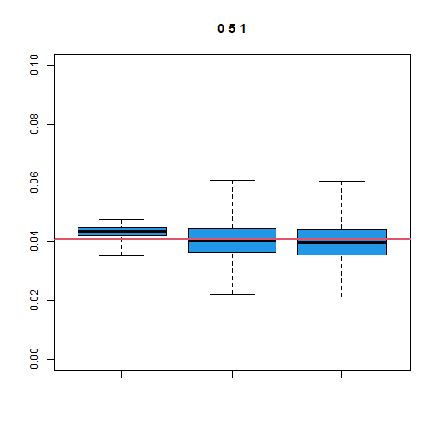
Figure 9. Effect of the informative prior in estimating frequencist’s variance in the $\rho=0$ case. The three panels shows the result for $(\alpha,\beta)=(5,1),(10,1),(20,1)$. In each panel, the Bayesian estimate $\mathrm{Var}_{\mathrm{pos}}[q]$, the simplified estimator $\hat{\Sigma}^{qq}$ by (13), and the original estimator $\hat{\Sigma}^{*}_{qq}$ by (12) are shown from the left to the right. The horizontal red line shows the true value of the frequencist’s variance. The boxplot is created by the base graphics of the R language with the ”range=0” option; the whisker in each boxplot spans the maximum and minimum of the plotted data.

Fig. 10 shows the result of an experiment performed in the over-dispersed $\rho=0.65$ case, where the model cannot correctly represent the true distribution. We perform the experiments with the beta prior of $(\alpha,\beta)=(1,1),(10,1),(20,1)$ and again compare $\mathrm{Var}_{\mathrm{pos}}[q]$, $\hat{\Sigma}^{qq}$ by (13) and $\hat{\Sigma}^{*}_{qq}$ by (12). The results are similar to the case $\rho=0$, except that the genuine Bayesian estimator $\mathrm{Var}_{\mathrm{pos}}[q]$ massively underestimate the variance in all cases of $\alpha$.

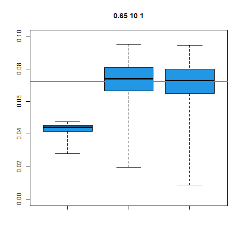
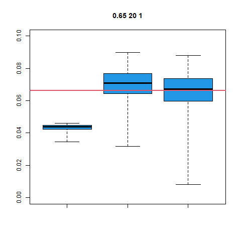
Figure 10. Effect of the informative prior in estimating frequencist’s variance in the $\rho=0.65$ case. The three panels shows the result for $(\alpha,\beta)=(1,1),(10,1),(20,1)$. In each panel, the Bayesian estimate $\mathrm{Var}_{\mathrm{pos}}[q]$, the simplified estimator $\hat{\Sigma}^{qq}$ by (13), and the original estimator $\hat{\Sigma}^{*}_{qq}$ by (12) are shown from the left to the right. The horizontal red line shows the true value of the frequencist’s variance. Other details are the same as in Fig. 9.

B.2. Consistency of (12) with $O(n)$ priors

Here, we will give an initiative argument that an alternative form (83) of the frequencist’s covariance formula, hence the original formula (12), is asymptotically correct in the setting of $O(n)$ priors. Equivalently, $n$ times (12) is a consistent estimator of $n$ times the frequencist’s covariance for $O(n)$ priors.

Preliminary

In the main text, we express an $O(n)$ prior as

(137) $$\log p(\theta)=n\Lambda\log\widetilde{p}(\theta)+\log p_{0}(\theta)+c.$$

Hereafter, we set $p_{0}(\theta)=1$ and ignore the normalizing constant $c$, which does not affect the result. Then, the prior and the resultant posterior is written as

(138) $$\log p(\theta)=n\Lambda\log\widetilde{p}(\theta),$$

and

(139) $$p(\theta\mid X^{n})=\frac{\exp\{\sum_{i=1}^{n}\ell(X_{i};\theta)+n\Lambda\log\widetilde{p}(\theta)\}}{\int\exp\{\sum_{i=1}^{n}\ell(X_{i};\theta^{\prime})+n\Lambda\log\widetilde{p}(\theta^{\prime})\}d\theta^{\prime}},$$

respectively.

We define $\theta_{0}^{*}=(\theta_{0,\alpha}^{*})$ as a solution of

(140) $$\mathbf{E}_{X}\left[\left.\frac{\partial}{\partial\theta_{\alpha}}\left\{\ell(X;\theta)+\Lambda\log\widetilde{p}(\theta)\right\}\right|_{\theta=\theta_{0}^{*}}\right]=0.$$

Using $\theta_{0}^{*}$, information matrices required in the following argument are defined as

(141) $$\mathcal{I}^{*}_{\alpha\beta}=\mathbf{E}_{X}\left[\left.\frac{\partial}{\partial\theta_{\alpha}}\left\{\ell(X;\theta)+\Lambda\log\widetilde{p}(\theta)\right\}\right|_{\theta=\theta_{0}^{*}}\left.\frac{\partial}{\partial\theta_{\beta}}\left\{\ell(X;\theta)+\Lambda\log\widetilde{p}(\theta)\right\}\right|_{\theta=\theta_{0}^{*}}\right],$$

(142) $$\mathcal{J}^{*}_{\alpha\beta}=-\mathbf{E}_{X}\left[\left.\frac{\partial^{2}}{\partial\theta_{\alpha}\partial\theta_{\beta}}\left\{\ell(X;\theta)+\Lambda\log\widetilde{p}(\theta)\right\}\right|_{\theta=\theta_{0}^{*}}\right].$$

The derivatives in (141) and (142) are evaluated at $\theta_{0}^{*}$ defined by (140), while derivatives in $\mathcal{I}$ and $\mathcal{J}$ given by (54) and (51) are evaluated at the projection $\theta_{0}$ to the model.

We also define empirical versions of these quantities. Let $\theta^{*}=(\theta^{*}_{\alpha})$ be a MAP estimate with the observations $X^{n}=(X_{i})$, which satisfies

(143) $$\sum_{i=1}^{n}\left.\frac{\partial}{\partial\theta_{\alpha}}\left\{\ell(X_{i};\theta)+\Lambda\log\widetilde{p}(\theta)\right\}\right|_{\theta=\theta^{*}}=0.$$

Then, we define

(144) $$\hat{\mathcal{I}}^{*}_{\alpha\beta}=\frac{1}{n}\sum_{i=1}^{n}\left\{\left.\frac{\partial}{\partial\theta_{\alpha}}\left\{\ell(X_{i};\theta)+\Lambda\log\widetilde{p}(\theta)\right\}\right|_{\theta=\theta^{*}}\left.\frac{\partial}{\partial\theta_{\beta}}\left\{\ell(X_{i};\theta)+\Lambda\log\widetilde{p}(\theta)\right\}\right|_{\theta=\theta^{*}}\right\},$$

(145) $$\hat{\mathcal{J}}^{*}_{\alpha\beta}=-\frac{1}{n}\sum_{i=1}^{n}\left.\frac{\partial^{2}}{\partial\theta_{\alpha}\partial\theta_{\beta}}\left\{\ell(X_{i};\theta)+\Lambda\log\widetilde{p}(\theta)\right\}\right|_{\theta=\theta^{*}}.$$

Finally, the relation (52) is generalize to

(146) $${\mathbf{E}}^{0}_{\mathrm{pos}}[(\theta_{\alpha}-\theta_{0,\alpha}^{*})(\theta_{\beta}-\theta_{0,\beta}^{*})] =\frac{(\mathcal{J}^{*})^{-1}_{\alpha\beta}}{n}+o_{p}(1/n),$$

(147) $$\mathbf{E}_{\mathrm{pos}}[(\theta_{\alpha}-\theta^{*}_{\alpha})(\theta_{\beta}-\theta^{*}_{\beta})] =\frac{(\hat{\mathcal{J}}^{*})^{-1}_{\alpha\beta}}{n}+o_{p}(1/n),$$

in the setting of $O(n)$ priors, where we denote an expectation with respect to the population version of the posterior (44) as ${\mathbf{E}}^{0}_{\mathrm{pos}}[\,\,\,]$. Note that $\mathbf{E}_{\mathrm{pos}}[\theta]=\theta^{*}+O_{p}(1/n)$ in our setting, but the error induced by replacing $\mathbf{E}_{\mathrm{pos}}[\theta]$ by $\theta^{*}$ in the right hand sides of formulae (146) is in the order of $O_{p}(1/n^{2})$. The same is also true in (147).

Sandwiched representation of frequencist’s covariance

Based on the equation (143) for the MAP estimate, we can derive an asymptotic representation of frequencist’s covariance in the setting of $O(n)$ priors. It is a straightforward generalisation of the classical result on the MLE, which corresponds to $\Lambda=0$. First, using the frequencist’s central limit theorem under the IID assumption of $X_{i}$s, we have

(148) $$\frac{1}{\sqrt{n}}\sum_{i=1}^{n}\left.\frac{\partial}{\partial\theta_{\alpha}}\left\{\ell(X_{i};\theta)+\Lambda\log\widetilde{p}(\theta)\right\}\right|_{\theta=\theta_{0}^{*}}\sim N(0,\mathcal{I}^{*}),$$

using (140) and (142). On the other hand, expanding the left hand side of the equation (143) around $\theta_{0}^{*}$ and transpose a term, we have

(149) $$\frac{1}{\sqrt{n}}\sum_{i=1}^{n}\left.\frac{\partial}{\partial\theta_{\alpha}}\left\{\ell(X_{i};\theta)+\Lambda\log\widetilde{p}(\theta)\right\}\right|_{\theta=\theta_{0}^{*}}$$

(150) $$=-\frac{1}{n}\sum_{\beta=1}^{k}\left[\left.\frac{\partial^{2}}{\partial\theta_{\alpha}\partial\theta_{\beta}}\left\{\sum_{i=1}^{n}\left\{\ell(X_{i};\theta)+\Lambda\log\widetilde{p}(\theta)\right\}\right\}\right|_{\theta=\theta_{0}^{*}}\!\!\!\sqrt{n}(\theta^{*}-\theta_{0}^{*})_{\beta}\right]+o_{p}(1)$$

Taking the variance of the both sides of (149) using (148), the frequencist’s covariance of $\theta^{*}$ is computed as

(151) $$\mathrm{Cov}_{X}[(\theta^{*}-\theta_{0}^{*})_{\alpha},(\theta^{*}-\theta_{0}^{*})_{\beta}]=\frac{1}{n}\sum_{\mathstrut\gamma,\gamma^{\prime}=1}^{k}({\mathcal{J}}^{*})^{-1}_{\alpha\gamma}\,{\mathcal{I}}^{*}_{\gamma\gamma^{\prime}}\,({\mathcal{J}}^{*})^{-1}_{\gamma^{\prime}\beta}\,+o(1/n).$$

For arbitrary statistics $A(\theta)$ and $B(\theta)$, the delta method gives

(152) $$\mathrm{Cov}_{X}[A(\theta^{*}),B(\theta^{*})]=\frac{1}{n}\sum_{\mathstrut\alpha,\beta=1}^{k}\sum_{\mathstrut\gamma,\gamma^{\prime}=1}^{k}(\mathcal{J}^{*})^{-1}_{\alpha\gamma}\,\mathcal{I}^{*}_{\gamma\gamma^{\prime}}\,(\mathcal{J}^{*})^{-1}_{\gamma^{\prime}\beta}\,\left.\frac{\partial A}{\partial\theta_{\alpha}}\right|_{\theta=\theta_{0}^{*}}\left.\frac{\partial B}{\partial\theta_{\beta}}\right|_{\theta=\theta_{0}^{*}}+o(1/n).$$

Substituting population versions $\mathcal{I}^{*}$ and $\mathcal{J}^{*}$ with empirical versions $\hat{\mathcal{I}}^{*}$ and $\hat{\mathcal{J}}^{*}$, and using the empirical values of the partial derivatives of $A$ and $B$, we also have

(153) $$\mathrm{Cov}_{X}[A(\theta^{*}),B(\theta^{*})]=\frac{1}{n}\sum_{\mathstrut\alpha,\beta=1}^{k}\sum_{\mathstrut\gamma,\gamma^{\prime}=1}^{k}(\hat{\mathcal{J}}^{*})^{-1}_{\alpha\gamma}\,\hat{\mathcal{I}}^{*}_{\gamma\gamma^{\prime}}\,(\hat{\mathcal{J}}^{*})^{-1}_{\gamma^{\prime}\beta}\,\left.\frac{\partial A}{\partial\theta_{\alpha}}\right|_{\theta=\theta^{*}}\left.\frac{\partial B}{\partial\theta_{\beta}}\right|_{\theta=\theta^{*}}+o_{p}(1/n).$$

In our settings, $\mathbf{E}_{\mathrm{pos}}[\theta]=\theta^{*}+O_{p}(1/n)$, but the error caused by the substitution of $\theta^{*}$ with $\mathbf{E}_{\mathrm{pos}}[\theta]$ in the left hand side of (153) is shown to be in the order of $O_{p}(1/n^{2})$. Then, we also have

(154) $$\qquad\mathrm{Cov}_{X}[\mathbf{E}_{\mathrm{pos}}[A],\mathbf{E}_{\mathrm{pos}}[B]]=\frac{1}{n}\sum_{\mathstrut\alpha,\beta=1}^{k}\sum_{\mathstrut\gamma,\gamma^{\prime}=1}^{k}(\hat{\mathcal{J}}^{*})^{-1}_{\alpha\gamma}\,\hat{\mathcal{I}}^{*}_{\gamma\gamma^{\prime}}\,(\hat{\mathcal{J}}^{*})^{-1}_{\gamma^{\prime}\beta}\,\left.\frac{\partial A}{\partial\theta_{\alpha}}\right|_{\theta=\theta^{*}}\left.\frac{\partial B}{\partial\theta_{\beta}}\right|_{\theta=\theta^{*}}+o_{p}(1/n).$$

Frequencist’s covariance formula in the settings of $O(n)$ priors

Now that we expand (83) around $\theta^{*}$ and use (147); it gives

(155) $$\mathrm{Cov}_{\mathrm{pos}}[A(\theta),\ell(X_{i};\theta)+\Lambda\log\widetilde{p}(\theta)]$$

(156) $$=\mathrm{Cov}_{\mathrm{pos}}\left[\sum_{\alpha=1}^{k}\left.\frac{\partial A}{\partial\theta_{\alpha}}\right|_{\theta=\theta^{*}}\!\!\!\!(\theta-\theta^{*})_{\alpha},\,\,\,\sum_{\beta=1}^{k}\left.\left\{\frac{\partial}{\partial\theta_{\beta}}\ell(X_{i};\theta)+\Lambda\log\widetilde{p}(\theta)\right\}\right|_{\theta=\theta^{*}}(\theta-\theta^{*})_{\beta}\right]+o_{p}(1/n)$$

(157) $$=\frac{1}{n}\sum_{\alpha,\beta=1}^{k}\left.\frac{\partial A}{\partial\theta_{\alpha}}\right|_{\theta=\theta^{*}}\left.\left\{\frac{\partial}{\partial\theta_{\beta}}\ell(X_{i};\theta)+\Lambda\log\widetilde{p}(\theta)\right\}\right|_{\theta=\theta^{*}}(\hat{\mathcal{J}}^{*})^{-1}_{\alpha\beta}+o_{p}(1/n).$$

Let us substitute this into (84) and use the definition (145), then we have

(158) $$\hat{\Sigma}^{**}_{AB} =\sum_{i=1}^{n}\mathrm{Cov}_{\mathrm{pos}}[A(\theta),\ell(X_{i};\theta)+\Lambda\log\widetilde{p}(\theta)]\,\mathrm{Cov}_{\mathrm{pos}}[B(\theta),\ell(X_{i};\theta)+\Lambda\log\widetilde{p}(\theta)]$$

(159) $$=\frac{1}{n}\sum_{\mathstrut\alpha,\beta=1}^{k}\sum_{\mathstrut\gamma,\gamma^{\prime}=1}^{k}(\hat{\mathcal{J}}^{*})^{-1}_{\alpha\gamma}\,\hat{\mathcal{I}}^{*}_{\gamma\gamma^{\prime}}\,(\hat{\mathcal{J}}^{*})^{-1}_{\gamma^{\prime}\beta}\,\left.\frac{\partial A}{\partial\theta_{\alpha}}\right|_{\theta=\theta^{*}}\left.\frac{\partial B}{\partial\theta_{\beta}}\right|_{\theta=\theta^{*}}+o_{p}(1/n),$$

which coincides with (154).

B.3. Effect of the centering and inconsistency of (13) with $O(n)$ priors

In the above, we argued that the frequencist’s covariance formulae (12) and (84) are correct in the order of $o_{p}(1/n)$ under the setting of $O(n)$ priors. Now, let us see that the order of the change from the simplified version (13) to the original version (12) in the strength $\Lambda$ of the prior. Rather unexpectedly, the difference between $\hat{\Sigma}^{**}_{AB}$ given by (84) and $\hat{\Sigma}_{AB}$ given by (13) is in the order $O_{p}(\Lambda^{2})$ and not $O_{p}(\Lambda)$ that naively expected. From the asymptotic equivalence between (12) and (84), this means that the difference between $\hat{\Sigma}^{*}_{AB}$ given by (12) and $\hat{\Sigma}_{AB}$ given by (13) is also $O_{p}(\Lambda^{2})$.

To see this, we start from (85) and rewrite it as

(160) $$\mathrm{Cov}_{\mathrm{pos}}\left[A(\theta),\sum_{i=1}^{n}\ell(X_{i};\theta)\right]=-n\Lambda\mathrm{Cov}_{\mathrm{pos}}[A(\theta),\log\widetilde{p}(\theta)]+o_{p}(1).$$

Then, a cross term in (84) is evaluated as

(161) $$\sum_{i=1}^{n}\mathrm{Cov}_{\mathrm{pos}}[A(\theta), \ell(X_{i};\theta)]\,\,\mathrm{Cov}_{\mathrm{pos}}[B(\theta),\Lambda\log\widetilde{p}(\theta)]$$

(162) $$=\Lambda\mathrm{Cov}_{\mathrm{pos}}\left[A(\theta),\sum_{i=1}^{n}\ell(X_{i};\theta)\right]\mathrm{Cov}_{\mathrm{pos}}[B(\theta),\log\widetilde{p}(\theta)]\,\,$$

(163) $$=\bigg{\{}\!\!-\Lambda^{2}n\,\mathrm{Cov}_{\mathrm{pos}}[A(\theta),\log\widetilde{p}(\theta)]+o_{p}(1)\bigg{\}}\,\,\mathrm{Cov}_{\mathrm{pos}}[B(\theta),\log\widetilde{p}(\theta)],$$

where the $$o_{p}(1) \{\,\} O(\Lambda) A(\theta) B(\theta)$$ term in is . Another cross term, where the role of and is reversed, is also evaluated in a similar way. On the other hand, the fourth term that does not contains the likelihood is evaluated as

(164) $$\sum_{i=1}^{n}\mathrm{Cov}_{\mathrm{pos}}[A(\theta), \Lambda\log\widetilde{p}(\theta)]\,\,\mathrm{Cov}_{\mathrm{pos}}[B(\theta),\Lambda\log\widetilde{p}(\theta)]$$

(165) $$=\Lambda^{2}n\mathrm{Cov}_{\mathrm{pos}}[A(\theta),\log\widetilde{p}(\theta)]\mathrm{Cov}_{\mathrm{pos}}[B(\theta),\log\widetilde{p}(\theta)].$$

Calculating $2\times\eqref{eq:cross}+\eqref{eq:diag}$ and add it to (13), we have

(166) $$\hat{\Sigma}^{**}_{AB}= \sum_{i=1}^{n}\mathrm{Cov}_{\mathrm{pos}}[A(\theta),\ell(X_{i};\theta)]\,\,\mathrm{Cov}_{\mathrm{pos}}[B(\theta),\ell(X_{i};\theta)]$$

(167) $$\qquad\qquad-\Lambda^{2}n\mathrm{Cov}_{\mathrm{pos}}[A(\theta),\log\widetilde{p}(\theta)]\mathrm{Cov}_{\mathrm{pos}}[B(\theta),\log\widetilde{p}(\theta)]+o_{p}(1/n),$$

which shows the difference between $\hat{\Sigma}^{**}_{AB}$ and $\hat{\Sigma}_{AB}$ defined by (13) is $O_{p}(\Lambda^{2})$, when we ignore $o_{p}(1/n)$ contributions.

This result suggests that the difference (13) between (12) is only relevant for highly informative priors. Most of the effect of informative priors is already contained in a simplified form (13) through the definition of the posterior covariance. From another viewpoint, however, the same result also indicates that the difference between (12) and (13) is in the order of $O_{p}(1/n)$, while (12) and (13) themselves are also in the order of $O_{p}(1/n)$. This means that $n$ times (13) is not a consistent estimator of $n$ times the frequencist’s covariance in the setting of $O(n)$ priors.

B.4. Model selection

Bias correction term of waic

Finally, we touch on related issues in model selection. As discussed in Vehtari et al., (2017) and Ninomiya, (2021), waic is not necessary to provide a unbiased estimator of the predictive loss in the setting of $O_{p}(n)$ prior. Iba and Yano, (2022) proposed a modification

(168) $$\sum_{i=1}^{n} \mathrm{Cov}_{\mathrm{pos}}\left[\ell(X_{i};\theta),\ell(X_{i};\theta)+\frac{1}{n}\log p(\theta)\right]$$

(169) $$=\sum_{i=1}^{n}\mathrm{Cov}_{\mathrm{pos}}[\ell(X_{i};\theta),\ell(X_{i};\theta)+\Lambda\log\widetilde{p}(\theta)]$$

of the bias correction term of waic, so as to provide a unbiased estimator up to the order of $o_{p}(1)$ in the setting of $O(n)$ priors; it has a form of the bias correction term of pcic (Iba and Yano, (2023, 2022)), and also can be seen as an analog of the form (84) of frequencist’s covariance formula. In Iba and Yano, (2022), the Gibbs predictive loss for a specific example is discussed, but it will be generalized to the predictive loss and also other models including singular models.

However, the difference of (168) and the bias correction term of waic

(170) $$\sum_{i=1}^{n}\mathrm{Var}_{\mathrm{pos}}[\ell(X_{i};\theta)]=\sum_{i=1}^{n}\mathrm{Cov}_{\mathrm{pos}}[\ell(X_{i};\theta),\ell(X_{i};\theta)]$$

is usually not so big, except that the effect of the informative prior is large. To explain this, let us see that the difference between (168) and (170) is in the order of $O(\Lambda^{2})$. If we set $A(\theta)=\Lambda\log\widetilde{p}(\theta)$ in (160), we can express the difference of (168) and (170) as

(171) $$\mathrm{Cov}_{\mathrm{pos}}\left[\sum_{i=1}^{n}\ell(X_{i};\theta),\Lambda\log\widetilde{p}(\theta)\right] =-n\Lambda\mathrm{Cov}_{\mathrm{pos}}[\Lambda\log\widetilde{p}(\theta),\log\widetilde{p}(\theta)]+o_{p}(1)$$

(172) $$=-\Lambda^{2}n\mathrm{Var}_{\mathrm{pos}}[\log\widetilde{p}(\theta)]+o_{p}(1),$$

which gives the desired result.

Note that the difference between tic and waic in regular models is usually of the order of $O(\Lambda)$ in the setting of $O(n)$ priors. Combined this to the above result, it indicates that considerable amount of the effect of the prior is already contained in the bias correction term of waic through the definition of the posterior variance.

Remark 9.

The relation (85) and (160) for the general $A(\theta)$ does not hold in singular models. However, we conjecture that a specialized form of (85)

(173) $$\mathrm{Cov}_{\mathrm{pos}}\left[\ell(X_{j};\theta),\sum_{i=1}^{n}\{\ell(X_{i};\theta)+\Lambda\log\widetilde{p}(\theta)\}\right]=o_{p}(1),$$

(174) $$\mathrm{Cov}_{\mathrm{pos}}\left[\log\widetilde{p}(\theta),\sum_{i=1}^{n}\{\ell(X_{i};\theta)+\Lambda\log\widetilde{p}(\theta)\}\right]=o_{p}(1)$$

will hold for singular models, and it is enough to show the difference between (168) and (170) is $O_{p}(\Lambda^{2})$.

A view from information matrices

In the above derivation, we directly treat the problem in a posterior covariance form and do not use expansion with parameters and hence not utilizing information matrices. Here we briefly discuss it from the viewpoint of modifications in information matrices.

Let us consider the population version for simplicity. Define a set of modified information matrices $\mathcal{I}^{\dagger}$ and $\mathcal{J}^{\dagger}$ by

(175) $$\mathcal{I}^{\dagger}_{\alpha\beta}=\mathbf{E}_{X}\left[\left.\frac{\partial}{\partial\theta_{\alpha}}\ell(X;\theta)\right|_{\theta=\theta_{0}^{*}}\left.\frac{\partial}{\partial\theta_{\beta}}\ell(X;\theta)\right|_{\theta=\theta_{0}^{*}}\right],$$

(176) $$\mathcal{J}^{\dagger}_{\alpha\beta}=-\mathbf{E}_{X}\left[\left.\frac{\partial^{2}}{\partial\theta_{\alpha}\partial\theta_{\beta}}\ell(X;\theta)\right|_{\theta=\theta_{0}^{*}}\right].$$

They have the same form as usual information matrices $\mathcal{I}$ and $\mathcal{J}$ but defined around $\theta=\theta_{0}^{*}$ instead of $\theta=\theta_{0}$.

A little computation gives

(177) $$\mathcal{I}^{*}_{\alpha\beta}=\mathcal{I}^{\dagger}_{\alpha\beta}-\Lambda^{2}\left.\frac{\partial}{\partial\theta_{\alpha}}\log\widetilde{p}(\theta)\right|_{\theta=\theta_{0}^{*}}\left.\frac{\partial}{\partial\theta_{\beta}}\log\widetilde{p}(\theta)\right|_{\theta=\theta_{0}^{*}},$$

while we can diretly obtain

(178) $$\mathcal{J}^{*}_{\alpha\beta}=\mathcal{J}^{\dagger}_{\alpha\beta}-\Lambda\left.\frac{\partial^{2}}{\partial\theta_{\alpha}\partial\theta_{\beta}}\log\widetilde{p}(\theta)\right|_{\theta=\theta_{0}^{*}}$$

These results show that the difference between $\mathcal{I}^{*}$ and $\mathcal{I}^{\dagger}$ is in the order $O(\Lambda^{2})$, while the difference between $\mathcal{J}^{*}$ and $\mathcal{J}^{\dagger}$ is in the order $O(\Lambda)$.

By using a Taylor expansion with parameters, we can show that the difference between pcic with a bias correction term (168) and tic is given by the following modifications: (1) change from $\hat{\theta}$ to $\theta^{*}$, (2) change from $\hat{\mathcal{J}}^{\dagger}$ to $\hat{\mathcal{J}}^{*}$, (3) change from $\hat{\mathcal{I}}^{\dagger}$ to $\hat{\mathcal{I}}^{*}$, where $\hat{\mathcal{I}}^{\dagger}$ and $\hat{\mathcal{J}}^{\dagger}$ are empirical versions of $\mathcal{I}^{\dagger}$ and $\mathcal{J}^{\dagger}$ defined around the MAP estimate $\theta=\theta^{*}$. The effect of (1) and (2) is already contained in the bias correction term (170) of waic; it is automatically included through the definition of the posterior means. Thus, the modification caused by (3) is the only source of the difference between waic and pcic; it is of the order of $O(\Lambda^{2})$ from the above-mentioned argument.

Appendix C Stochastic expansion of the predictive and empirical loss

In Sec. 3, we showed two approaches to the essential subspace. Here we take a look at the problem from the view of predictive performance, as the third approach to the essential subspace. It is, however, more intricate than the previous approaches, so that we only provide conjectured results and a post hoc justification of the formulae (179),(181), and (189) in the case of regular models where the effect of the prior can be ignored. Treating them using the Bayesian IJK is left for future studies, as well as mathematically rigorous proofs.

C.1. Stochastic expansion

First, we define notations and settings: $X^{n}$ is current data used to define $\mathbf{E}_{\mathrm{pos}}[\,\,\,]$, $\mathrm{Var}_{\mathrm{pos}}[\,\,\,]$ and $\mathrm{Cov}_{\mathrm{pos}}[\,\,\,]$. $Y^{n}$ and $Z^{n}$ are both a dummy variable that represents a fresh sample from the population, but we use different notations to stress that $Z^{n}$ is test data to define predictive loss. The posterior variance defined by the posterior with the data $Y$ is denoted as $\mathrm{Var}_{\mathrm{pos}}^{Y}[\,\,\,]$. We assume that the effect of the prior can be ignored except in Sec. C.5.

The relevant expressions for the predictive and empirical loss are given as

(179) $$\qquad n\mathbf{E}_{Z}\big{[}\log\mathbf{E}_{\mathrm{pos}}[p(Z;\theta)]\big{]}\,=\,\, n\mathbf{E}_{Z}[\ell(Z;\theta_{0})]-\frac{k}{2}+\frac{1}{2}\mathbf{E}_{Y}[\,\mathrm{Var}_{\mathrm{pos}}^{Y}[\ell(Y;\theta)]\,]$$

(180) $$-\frac{1}{2}\sum_{i,j=1}^{n}\mathrm{Cov}_{\mathrm{pos}}[\ell(X_{i};\theta),\ell(X_{j};\theta)]\,\,\,+o_{p}(1),$$

(181) $$\qquad\sum_{i=1}^{n}\log\mathbf{E}_{\mathrm{pos}}[p(X_{i};\theta)]\,=\,\, \sum_{i=1}^{n}\ell(X_{i};\theta_{0})\,\,-\frac{k}{2}+\frac{1}{2}\mathbf{E}_{Y}[\,\mathrm{Var}_{\mathrm{pos}}^{Y}[\ell(Y;\theta)]\,]$$

(182) $$+\frac{1}{2}\sum_{i,j=1}^{n}\mathrm{Cov}_{\mathrm{pos}}[\ell(X_{i};\theta),\ell(X_{j};\theta)]\,\,\,+o_{p}(1).$$

Here we derive (179) for regular models using the expression (125) in the appendix A.3 and asymptotic equivalence of $K_{MF}$ and $K_{W}$. For regular models, stochastic expansion of the log-likelihood and related quantities are well studied (Konishi and Kitagawa, (2008); Watanabe, (2018); Ninomiya, (2021)). As given in the theorem 6 of Watanabe, (2018), a stochastic expansion the predictive loss for a regular Bayesian model is expressed as

(183) $$n\mathbf{E}_{Z}[\log\mathbf{E}_{\mathrm{pos}}^{\mathrm{Y}}[p(Z;\theta)]]=\, n\mathbf{E}_{Z}[\log p(Z;\theta_{0})]-\frac{k}{2}+\frac{1}{2}\mathrm{tr\,}\mathcal{I}\mathcal{J}^{-1}-\frac{1}{2}\|\Xi\|^{2}+o_{p}(1),$$

where $\Xi=(\Xi_{\gamma})$ is a random variable given by

(184) $$\Xi_{\gamma}=\sum_{i=1}^{n}\sum_{\alpha=1}^{k}(\mathcal{J}^{-1/2})_{\gamma\alpha}\frac{\partial}{\partial\theta_{\alpha}}\ell(X_{i};\theta)\bigg{|}_{\theta=\theta_{0}}.$$

Let us compare (179) with (183). First, it is easy to show that the constants are the same within $o_{p}(1)$ error: $-\frac{k}{2}$ is common in both equations, and the asymptotic relation $\mathrm{Var}_{\mathrm{pos}}^{Y}[\ell(Y;\theta)]=\mathrm{tr\,}\mathcal{I}\mathcal{J}^{-1}$ is well known (Watanabe, (2018)). Then, the rest of the problem is to show the convergence in law between the variables

(185) $$\sum_{i,j=1}^{n}\mathrm{Cov}_{\mathrm{pos}}[\ell(X_{i};\theta),\ell(X_{j};\theta)]$$

and

(186) $$\|\Xi\|^{2}=\sum_{\gamma=1}^{k}\left(\sum_{i=1}^{n}\sum_{\alpha=1}^{k}(\mathcal{J}^{-1/2})_{\gamma\alpha}\frac{\partial}{\partial\theta_{\alpha}}\ell(X_{i};\theta)\bigg{|}_{\theta=\theta_{0}}\right)^{2},$$

when both are considered as a random variable induced by the repeated sampling of $X^{n}$ from the population. If we assume the change from $\theta_{0}$, $\mathcal{J}$ to $\hat{\theta}$, $\hat{\mathcal{J}}$ in the right hand side of (184) does not affect the distribution of $\|\Xi\|^{2}$ in the leading order and use the asymptotic equivalence of $K_{MF}(X_{i},X_{j})$ to $K_{W}(X_{i},X_{j})$, it follows from (125). We can also derive (181) in a similar way.

C.2. Approximate bootstrap

Next, we consider an “approximate bootstrap” version of (179) and (181). To do this, we introduce a set of auxiliary random variables $\eta^{n}=(\eta_{i})$. Each $\eta_{i}$ corresponds to $R_{i}-1$ in the usual bootstrap, where $(R_{i})$ is a multinomial random number. Hereafter, however, we regard them as independent random numbers that obeys $\eta_{i}\sim N(0,1)$, which is enough for a theoretical consideration.

We will introduce $\eta^{n}=(\eta_{i})$ to (179) and (181) according to the initiative rule of the bootstrap, where true values and observed values are replaced by observed values and bootstrapped values, respectively. After the observed likelihood $\ell(X_{i};\theta)$ is replaced by the bootstrapped likelihood $(1+\eta_{i})\ell(X_{i};\theta)$ in the posterior covariance, the relation

(187) $$\mathrm{Cov}_{\mathrm{pos}}[ (1+\eta_{i})\ell(X_{i};\theta),(1+\eta_{j})\ell(X_{j};\theta)]=$$

(188) $$\mathrm{Cov}_{\mathrm{pos}}[\ell(X_{i};\theta),\ell(X_{j};\theta)]+\mathrm{Cov}_{\mathrm{pos}}[\ell(X_{i};\theta),\ell(X_{j};\theta)]\,\eta_{i}\eta_{j}+o_{p}(1/n)$$

is used to simplify the formula; this relation is derived from (81). Hence we have the following set of equations, each of which gives a Bayesian IJK version of the bootstrap approximation to the right hand sides of (179) and (181):

(189) $$n\mathbf{E}_{Z}\big{[}\log\mathbf{E}_{\mathrm{pos}}[p(Z;\theta)]\big{]} -\frac{1}{2}\sum_{i,j=1}^{n}\mathrm{Cov}_{\mathrm{pos}}[\ell(X_{i};\theta),\ell(X_{j};\theta)]\,\eta_{i}\eta_{j}$$

(190) $$\sum_{i=1}^{n}\log\mathbf{E}_{\mathrm{pos}}[p(X_{i};\theta)] +\sum_{i=1}^{n}\ell(X_{i};\theta_{0})\,\eta_{i} +\frac{1}{2}\sum_{i,j=1}^{n}\mathrm{Cov}_{\mathrm{pos}}[\ell(X_{i};\theta),\ell(X_{j};\theta)]\,\eta_{i}\eta_{j}.$$

In (190), $\ell(X_{i};\theta_{0})$ in the second term still contains unknown $\theta_{0}$ and not completely replaced by its empirical estimate; we will discuss it later. Also, note that (189) and (190) are considered as a random variable induced by $\eta^{n}$, whereas the right hand sides of (179) and (181) are considered as random variables induced by the sample $X^{n}$ randomly extracted from the population. The convergence of the bootstrap method is interpreted as a convergence in law between these distributions.

Let us give a rough sketch of deriving the convergence of (189) to (179) in this sense. If we define

(191) $$\Xi^{B}_{\gamma}=\sum_{i=1}^{n}\sum_{\alpha=1}^{k}(\mathcal{J}^{-1/2})_{\gamma\alpha}\frac{\partial}{\partial\theta_{\alpha}}\ell(X_{i};\theta)\bigg{|}_{\theta=\theta_{0}}\eta_{i},$$

an argument similar to the previous subsection shows the expression

(192) $$\sum_{ij}\mathrm{Cov}_{\mathrm{pos}}[\ell(X_{i};\theta),\ell(X_{j};\theta)]\,\eta_{i}\eta_{j}$$

is asymptotically equals to $\|\Xi^{B}\|^{2}$ as a random variable.

On the other hand, the definitions (184) and (191) indicate that

• $\Xi$    obeys $N\big{(}0,\mathcal{J}^{-1/2}\mathcal{I}\mathcal{J}^{-1/2}\big{)}$ as a random variable induced by $X^{n}$,

• $\Xi^{B}$ obeys $N\big{(}0,\mathcal{J}^{-1/2}\hat{\mathcal{I}}\mathcal{J}^{-1/2}\big{)}$ as a random variable induced by $\eta^{n}$.

The first relation is asymptotic, but the second one is exact after replacing $\hat{\mathcal{J}}$ to $\mathcal{J}$ in (191). Using these relations and asymptotic equivalence between $\hat{\mathcal{I}}$ and $\mathcal{I}$, it is shown that the distribution of $\|\Xi^{B}\|^{2}$ induced by $\eta^{n}$ converges to the distribution of $\|\Xi\|^{2}$ induced by $X^{n}$. Hence, the distribution of (192) also converges to the distribution of $\|\Xi\|^{2}$ in the same sense. This indicates the desired relation between (189) and (179).

In a similar way, we can show that the convergence of the distribution of (190) to the distribution of the right hand side of (181), while manipulating the formula (190) requires a bit more consideration, since the same $\eta^{n}$ appeared in two different terms.

C.3. Essential subspace in approximate bootstrap

In (189) and (190), the expression

(193) $$\frac{1}{2}\sum_{i,j=1}^{n}\mathrm{Cov}_{\mathrm{pos}}[\ell(X_{i};\theta),\ell(X_{j};\theta)]\,\eta_{i}\eta_{j},\,\,\,\eta_{i}\sim N(0,1)$$

is identical to $\frac{1}{2}\sum_{i,j=1}^{n}W_{ij}\eta_{i}\eta_{j}$. Then, it is straightforward to apply the idea of the essential subspace and (193) is expressed as

(194) $$\frac{1}{2}\sum_{a=1}^{a_{M}}\lambda_{\alpha}\eta_{a}^{2},\,\,\,\eta_{a}\sim N(0,1),$$

where $\{\lambda_{\alpha}\},\alpha=1,\ldots,a_{M}$ are effectively nonzero eigenvalues of the matrix $W=(W_{ij})$. The distribution of the random variable (194) is a weighted chi-square distribution, where the weights are defined by the eigenvalues $\{\lambda_{\alpha}\}$ of the matrix $W$.

C.4. Application

Unfortunately, there is a difficulty to apply (190) to measure the uncertainty of the model selection in practice. This is caused by the sensitivity of bootstrap variances of (190) to the values of $\ell(X_{i};\theta_{0})$, which relies on the unknown value $\theta_{0}$. Replacing terms that contain $\ell(X_{i};\theta_{0})$ with their empirical estimates causes instability when we consider the difference of the loss for a nested pair of models, but removing these terms is inadequate in a non-nested case. This is a common problem that arises when the uncertainty in the model selection is considered, and not particularly related to the posterior covariance representation discussed here. Related mathematical problems are discussed in Babu, (1984); Chen and Fang, (2019).

A way to partially solve the problem is to treat a nested and non-nested case (and possibly “partially nested” cases) separately. In this line of ideas, Vuong, (1989) developed a statistical test to compare the productivity of models according to the KL-divergence (Vuong closeness test). For a nested pair of the models, a Bayesian version of such test leads to another eigenvalue problem of the matrix

(195) $$\mathcal{V}_{ij}=\mathrm{Cov}_{\mathrm{pos}}^{(1)}[\log p_{1}(X_{i}\mid\theta_{1}),\log p_{1}(X_{j}\mid\theta_{1})]-\mathrm{Cov}_{\mathrm{pos}}^{(2)}[\log p_{2}(X_{i}\mid\theta_{2}),\log p_{2}(X_{j}\mid\theta_{2})],$$

where $p_{1}(X_{i}\mid\theta_{1})$ and $p_{2}(X_{i}\mid\theta_{2})$ are likelihoods of the models and $\mathrm{Cov}_{\mathrm{pos}}^{(1)}[\,\,\,]$ and $\mathrm{Cov}_{\mathrm{pos}}^{(2)}[\,\,\,]$ denote the posterior covariance defined by these likelihoods and appropriate priors. Further researches in this direction is left for future studies.

C.5. $O(n)$ priors

The effect of informative prior in the analysis of the predictive and empirical loss is more intricate than the general case of the Bayesian IJK and a mere introduction is given here. First, if we are interested in the evaluation of a modified loss function

(196) $$\ell(X;\theta)+\frac{1}{n}\log p(\theta),$$

it is reasonable to replace the matrix $\mathrm{Cov}_{\mathrm{pos}}[\ell(X_{i};\theta),\ell(X_{j};\theta)]$ with another symmetric matrix

(197) $$\mathrm{Cov}_{\mathrm{pos}}\left[\ell(X_{i};\theta)+\frac{1}{n}\log p(\theta),\ell(X_{j};\theta)+\frac{1}{n}\log p(\theta)\right].$$

This type of the loss function have been treated in the literature (Murata et al., (1994)), but it seems a rare choice. In most applications, we are interested in original loss function $\ell(X_{i};\theta)$; in this case, the corresponding matrix may be modified to a form

(198) $$\mathrm{Cov}_{\mathrm{pos}}\left[\ell(X_{i};\theta),\ell(X_{j};\theta)+\frac{1}{n}\log p(\theta)\right],$$

whose diagonal term is the bias correction term (168) of pcic. Unfortunately, it is no longer a symmetric matrix that defines a reproducing kernel and we need some other strategy to employ the kernel framework.

Let us look at it from the viewpoint of the stochastic expansion of the loss. Utilizing the original loss function, we conjecture that the bootstrap version (189) and (190) of the stochastic expansions will be modified in the $O(n)$ setting of priors as follows:

(199) $$n\mathbf{E}_{Z}\big{[}\log\mathbf{E}_{\mathrm{pos}}[p(Z;\theta)]\big{]}+\sum_{i=1}^{n}{\mathrm{Cov}_{\mathrm{pos}}\left[\sum_{m=1}^{n}\ell(X_{m};\theta),\ell(X_{i};\theta)\right]\eta_{i}}$$

(200) $$+\frac{1}{2}\sum_{i,j=1}^{n}{\mathcal{K}_{\mathrm{pos}}}\left[\sum_{m=1}^{n}\ell(X_{m};\theta),\ell(X_{i};\theta),\ell(X_{j};\theta)\right]\eta_{i}\eta_{j}.$$

(201) $$\sum_{i=1}^{n}\log\mathbf{E}_{\mathrm{pos}}[p(X_{i};\theta)]+\sum_{i=1}^{n}\ell(X_{i};\theta_{0})\,\eta_{i}+\sum_{i=1}^{n}{\mathrm{Cov}_{\mathrm{pos}}\left[\sum_{m=1}^{n}\ell(X_{m};\theta),\ell(X_{i};\theta)\right]\eta_{i}}$$

(202) $$+\sum_{i,j=1}^{n}\mathrm{Cov}_{\mathrm{pos}}[\ell(X_{i};\theta),\ell(X_{j};\theta)]\,\eta_{i}\eta_{j}+\frac{1}{2}\sum_{i,j=1}^{n}{\mathcal{K}_{\mathrm{pos}}}\left[\sum_{m=1}^{n}\ell(X_{m};\theta),\ell(X_{i};\theta),\ell(X_{j};\theta)\right]\eta_{i}\eta_{j}.$$

The stochastic expansions (199) and (201) contain different quadratic forms of $\eta_{i}$s, hence the essential subspace is not common between them. Using (81) and another relation

(203) $${\mathcal{K}_{\mathrm{pos}}}\left[\sum_{m=1}^{n}\ell(X_{m};\theta),\ell(X_{i};\theta),\ell(X_{j};\theta)\right]=-\,\mathrm{Cov}_{\mathrm{pos}}[\ell(X_{i};\theta),\ell(X_{j};\theta)]+o_{p}(1/n),$$

which holds in the $O(1)$ setting of priors, we can show that (199) and (201) reduce to (189) and (190) in the case of non-informative priors; details will be discussed elsewhere.

References

- Babu, (1984) Babu, G. J. (1984). Bootstrapping statistics with linear combinations of chi-squares as weak limit. Sankhyā: The Indian Journal of Statistics, Series A, 46(1):85–93.
- Bradlow and Zaslavsky, (1997) Bradlow, E. and Zaslavsky, A. M. (1997). Case influence analysis in Bayesian inference. Journal of Computational and Graphical Statistics, 6:314–331.
- Cardot and Degras, (2017) Cardot, H. and Degras, D. (2017). Online principal component analysis in high dimension: Which algorithm to choose? International Statistical Review, 86(1):29–50.
- Carlin and Louis, (2008) Carlin, B. P. and Louis, T. A. (2008). Bayesian Methods for Data Analysis , 3rd Edition. Chapman and Hall/CRC.
- Chen and Fang, (2019) Chen, Q. and Fang, Z. (2019). Inference on functionals under first order degeneracy. Journal of Econometrics, 210(2):459–481.
- Efron, (2015) Efron, B. (2015). Frequentist accuracy of Bayesian estimates. Journal of the Royal Statistical Society. Series B, 77:617–646.
- Gelfand et al., (1992) Gelfand, A., Dey, D., and Chang, H. (1992). Model determination using predictive distributions with implementation via sampling-based methods. In Bernardo, J., Berger, J., Dawid, A., and Smith, A., editors, Bayesian Statistics, pages 147–167. Oxford University Press.
- Gelman et al., (2013) Gelman, A., Carlin, J., Stern, H., Dunson, D., Vehtari, A., and Rubin, D. (2013). Bayesian Data Analysis, 3rd Edition. Chapman and Hall/CRC.
- Gelman et al., (2015) Gelman, A., Lee, D., and Guo, J. (2015). Stan: A probabilistic programming language for bayesian inference and optimization. Journal of Educational and Behavioral Statistics, 40(5):530–543.
- Giordano, (2020) Giordano, R. (2020). Effortless frequentist covariances of posterior expectations. https://mc-stan.org/events/stancon2020/. a video on YouTube.