Fast and Interpretable Mortality Risk Scores
for Critical Care Patients

Abstract

Prediction of mortality in intensive care unit (ICU) patients is an important task in critical care medicine. Prior work in creating mortality risk models falls into two major categories: domain-expert-created scoring systems, and black box machine learning (ML) models. Both of these have disadvantages: black box models are unacceptable for use in hospitals, whereas manual creation of models (including hand-tuning of logistic regression parameters) relies on humans to perform high-dimensional constrained optimization, which leads to a loss in performance. In this work, we bridge the gap between accurate black box models and hand-tuned interpretable models. We build on modern interpretable ML techniques to design accurate and interpretable mortality risk scores. We leverage the largest existing public ICU monitoring datasets, namely the MIMIC III and eICU datasets. By evaluating risk across medical centers, we are able to study generalization across domains. In order to customize our risk score models, we develop a new algorithm, GroupFasterRisk, which has several important benefits: (1) it uses hard sparsity constraint, allowing users to directly control the number of features; (2) it incorporates group sparsity to allow more cohesive models; (3) it allows for monotonicity correction on models for including domain knowledge; (4) it produces many equally-good models at once, which allows domain experts to choose among them. GroupFasterRisk creates its risk scores within hours, even on the large datasets we study here. GroupFasterRisk’s risk scores perform better than risk scores currently used in hospitals, and have similar prediction performance to black box ML models (despite being much sparser). Because GroupFasterRisk produces a variety of risk scores and handles constraints, it allows design flexibility, which is the key enabler of practical and trustworthy model creation.

1 Introduction

Prediction of in-hospital mortality risk is a crucial task in medical decision-making [1, 2, 1, 3], assisting medical practitioners to better estimate the patient’s state and allocate resources appropriately for better treatment, disease staging, and triage support [4, 5, 6]. Mortality risk is usually performed with severity of illness risk scores, where each feature is transformed into an integer-valued component function based on its degree of deviation from normal values, and a nonlinear function transforms the sum of component functions into an estimate of risk. Risk scores are designed to be easy to understand, troubleshoot, and use in practice. A method for constructing more accurate (but still interpretable) severity of illness risk scores could save lives and assist with better allocation of resources.

The severity of illness risk scores have been constructed in various ways since the early 1980’s, starting with the APACHE [7], SOFA [8, 9], APACHE II [10], and SAPS [11] scores, which are still in use presently, as well as the more recent APACHE IV [12] score. All of these scores were built using a combination of basic statistical techniques and domain expertise. Statistical hypothesis testing was generally used for variable selection, and techniques like logistic regression and locally weighted least squares [13] were often used for combining variables. This process left many manual choices for analysts: at what significance level should we stop including variables? Of the many features selected by hypothesis testing, how should we choose which ones would be included? How should the cutoffs for risk increases for each variable be determined? How do the risk scores from logistic regression become integer point values that doctors can easily sum, troubleshoot, and understand? While a variety of heuristics have been used to answer these questions, ideally, the answers would be determined automatically by an algorithm that optimizes predictive performance; humans, even equipped with heuristics, are not naturally adept at high-dimensional constrained optimization. It is particularly important that these models are sparse in the number of features so they are easy to calculate in practice. For instance, because APACHE scores require 142 features, they are potentially more error-prone, and not all features may be available for every patient.

Recently, more modern statistical and machine learning (ML) approaches have been used to create interpretable models for predicting mortality without the need for manual intervention. Specifically, the OASIS score [14] was built from a process consisting of a genetic algorithm [15] that selects a subset of predictive variables to be included in the system, particle swarm optimization [16] to determine integer scores for each decile of the variables, and logistic regression for transforming integer scores into probability predictions. However, genetic algorithm and particle swarm optimization approaches can be insufficient, leading to the possibility of improved performance using other techniques.

State-of-the-art black box ML approaches have been applied to the mortality risk prediction, aiming to improve predictive performance [17, 18, 19, 20, 21, 22]. For instance, OASIS+ researchers [18] used a variety of black box ML algorithms (such as random forest [23] and XGBoost [24]) on OASIS features to develop models that mostly outperform other severity of illness scores such as OASIS and SAPS II. The black box models combine variables in highly nonlinear ways, and are not easy to troubleshoot or use in practice, which is why, to the best of our knowledge, OASIS+ models have not been adopted for mortality risk prediction in ICUs. Black box models with “explanations” are also insufficient [25]. However, it is useful to benchmark with black box models to determine whether there is a gap in accuracy between interpretable and black box models. In this work, we also benchmark against black box accuracy and show that our new techniques are able to close the gap.

In this work, we introduce GroupFasterRisk— an interpretable machine learning algorithm capable of producing a set of diverse, high-quality risk scores with equally high predictive accuracy — to generate severity of illness scores. GroupFasterRisk automates feature selection, cutoffs for risk increases, and integer weight assignments. Our approach optimizes more carefully than the approach of OASIS and another risk-score generation method called AutoScore [26], is much more scalable than its predecessor RiskSLIM [27, 28], and is more customizable than its predecessor FasterRisk [29]. GroupFasterRisk optimization process yields higher-quality interpretable models than competitors; in fact, its models are as predictive as black box models. Our contributions are as follows:

• We propose a new framework, namely GroupFasterRisk, for the automatic creation of severity of illness scores using an ML algorithm. GroupFasterRisk produces accurate risk scores within a relatively short time on a small personal laptop while giving users the flexibility to use an arbitrary number of physiological measurements and sparsity constraints. GroupFasterRisk incorporates group sparsity and monotonicity constraints in its optimization process to allow for the creation of more cohesive and interpretable models for medical applications.

• Using GroupFasterRisk, we provide multiple high-quality mortality risk scores with varying sparsity constraints and a number of variables, which could be potentially applied in a critical care setting to provide mortality risk predictions.

• Through extensive out-of-distribution (OOD) testing (at hospitals not used for training), we demonstrate that risk scores created by GroupFasterRisk outperform OASIS and SAPS II and are similar in performance to APACHE IV/IVa while using much fewer variables, thus being much easier to troubleshoot and use. Results also demonstrate that our approach generalizes OOD and even performs similarly to black box ML models.

• Our proposed method performs well across subpopulations, exceeding the performance of OASIS and SOFA on sepsis/septicemia patients, acute myocardial infarction patients, heart failure patients, and acute kidney failure patients. Its scores are comparable to SAPS II and APACHE IV, exceeding their performance in some subpopulations.

• We show that GroupFasterRisk selects more useful features than OASIS for predicting patient outcomes. We also show that it produces fair and well-calibrated predictions across different ethnic and gender groups across the United States.

2 Results

This work proposes the algorithm GroupFasterRisk for building risk scores, and applies it to mortality risk prediction. A risk score is a sparse generalized additive model with integer coefficients. Figure 1 provides a risk score for all-cause mortality learned by GroupFasterRisk on our processed version of the MIMIC III dataset with a group sparsity constraint of 15 features. GroupFasterRisk selects features by optimizing logistic loss using $\ell_{0}$ minimization as discussed in Section 2.1.2.

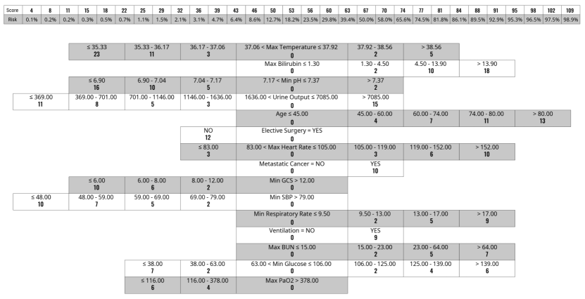
Figure 1: Risk score produced by GroupFasterRisk. This model has a group sparsity of 15 (GFR-15), which means that the model uses 15 features with multiple splits per feature. The total number of splits is regularized using per-feature sparsity. Max and Min represent the maximum and minimum value of the measurement over the first 24 hours of a patient’s ICU stay.

2.1 Study Overview and Design

2.1.1 Datasets Description and Evaluation Metrics

Datasets: To study the task of mortality prediction, we consider the Medical Information Mart for Intensive Care III (MIMIC III) dataset [30] and the eICU Collaborative Research Database (eICU) [31]. MIMIC III contains clinical data for 38,597 distinct patients admitted to the clinical care units of the Beth Israel Deaconess Medical Center between 2001 and 2012, and eICU contains clinical data for 139,367 patients admitted to the critical care units of medical centers across the United States between 2014 and 2015.

Train/Test Setup: To train our models, we created features from the MIMIC III dataset using physiological measurements, lab measurements, and patient comorbidities. We performed nested cross-validation for parameter tuning and internal evaluation on the MIMIC III dataset. To test the generalization ability of our model, we used the eICU dataset for out-of-distribution (OOD) testing. We provide the details of our preprocessing and cohort selection for both datasets in Section A.1 and Section 4.

Performance Evaluation Metrics: We adopt the area under the receiver-operating characteristic curve (AUROC) and the area under the precision-recall curve (AUPRC) as our metrics for predictive accuracy. Since our datasets are highly imbalanced, AUROC alone may not accurately capture the performance of models on the minority class (expired patients) [32]; we use AUPRC as an additional evaluation metric to provide a more complete view of the predictive accuracy. The AUPRC score becomes important when medical practitioners need to prioritize patients with more critical conditions (positive class), as it evaluates the model’s ability to correctly classify the positive class in scenarios where it is much smaller than the negative class.

Sparsity Evaluation Metric: We define a model’s sparsity informally as a way of measuring the model’s size. For linear models such as logistic regression, explainable boosting machine (EBM) [33], AutoScore [26], and GroupFasterRisk, sparsity is the total number of coefficients, intercepts, and multipliers. For tree-based models like XGBoost [34], AdaBoost [35], and Random Forest [23], sparsity is the number of splits in all trees.

Calibration Evaluation Metrics: In mortality risk prediction, even if a model demonstrates high accuracy based on AUROC and AUPRC, it may not provide precise risk probability estimates. This is because they are rank statistics [36]. We evaluate reliability based on Brier score, Hosmer-Lemeshow $\chi^{2}$ statistics (HL $\chi^{2}$), and the standardized mortality ratio (SMR) [37, 38]. We use $C$-statistics for HL $\chi^{2}$, calculated from deciles of predicted probabilities. Unless mentioned otherwise, we use paired $t$-test for statistical testing, and the p-value is denoted with $p$.

2.1.2 GroupFasterRisk and Baseline Methods used for Comparison

GroupFasterRisk produces high-quality risk scores. It improves over its predecessor FasterRisk [29], which is a data-driven ML approach that learns high-quality scoring systems within a relatively short time (Figure 6(b)). Although FasterRisk achieves near-optimal performance, it has limitations: (1) it does not allow users to add hard constraints on the number of features used in the model; (2) it does not incorporate monotonicity constraints, which means it can learn unrealistic component functions (see examples of ablation study in Section C.1). To handle (1) and (2), GroupFasterRisk includes group sparsity and monotonicity correction. The group sparsity option allows users to define any arbitrary partition (grouping) of the features and regularize all of these features towards 0 simultaneously. The monotonicity correction ensures that the models are nondecreasing (or nonincreasing) along one variable. GroupFasterRisk then produces multiple diverse, equally accurate models obeying this constraint. The trained models could be easily visualized with a risk scorecard representation using our software. We discuss group sparsity and monotonic correction in Methods (Section 4.1 and Section 4.4 correspondingly).

Figure 2: GroupFasterRisk algorithm workflow. We first find a near-optimal solution for a sparse logistic regression problem without the integer constraints. This solution is used in the second stage to search for a diverse pool of sparse continuous solutions that also satisfy various constraints (still ignoring the integer constraints) while having similar predictive accuracy. We subsequently select the top $m$ solutions and apply a rounding search subroutine to obtain integer-valued solutions. Our algorithm is carefully designed to ensure that the integer-valued solutions maintain similar performance to real-valued solutions.

Figure 2 summarizes the algorithmic approach of GroupFasterRisk, which returns scorecard displays in three steps. We begin by solving the sparse logistic regression problem, producing a near-optimal, real-valued sparse solution. This single solution is then used to find multiple diverse solutions with similar logistic loss [39, 40, 41]). Finally, a rounding subroutine is applied to all solutions to transform real-valued coefficients into integers, creating multiple risk scorecards that practitioners can choose from. Monotonicity correction can be optionally incorporated in all three steps. Notably, compared to other scoring system methods, GroupFasterRisk can produce high-quality risk scores for MIMIC III within a few hours on a personal laptop (we discuss more on the run time of GroupFasterRisk in Section 2.2).

To demonstrate the superiority of our proposed method, we compare it with two sets of baselines. The first set includes existing severity of illness scores such as the Oxford Acute Severity of Illness Score (OASIS) [14], Simplified Acute Physiology Score II (SAPS II) [42], Sequential Organ Failure Assessment (SOFA) [8], and Acute Physiology and Chronic Health Evaluation IV/IVa (APACHE IV/IVa) [12]. We did not consider qSOFA [9] because the score was originally developed for organ failure assessment, which may not directly predict in-hospital mortality. However, studies [43] have shown that SOFA can outperform qSOFA on in-hospital mortality prediction tasks, so we include SOFA. The second set of baselines consists of widely used ML algorithms, such as Logistic Regression, EBM [44], Random Forest [23], AdaBoost [35], and XGBoost [24]. (A predecessor of GroupFasterRisk is RiskSLIM [27, 28], which has been tested extensively with FasterRisk, so we do not include it here as it is much more computationally expensive.) We further categorize these baselines into two groups based on the number of variables: sparse (no more than 17 variables, including OASIS, SOFA, and SAPS II) and not sparse (more than 40 variables, like APACHE IV/IVa). Our goal is to develop sparse models since they are highly interpretable [39], but we still evaluate GroupFasterRisk models against APACHE IV/IVa. For fair comparison, we set the same or lower group sparsity constraint (number of variables) on GroupFasterRisk than the baselines across all the experiments. For conciseness, we denote GroupFasterRisk models with the prefix GFR and group sparsity as the suffix. For instance, a GroupFasterRisk model trained with a group sparsity of 10 is GFR-10.

2.2 All-cause Mortality Prediction

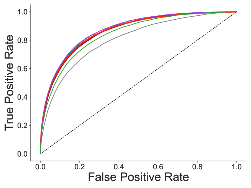
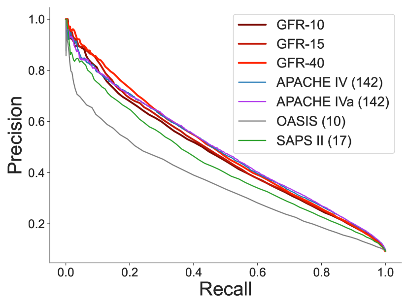
(a)

(a) GroupFasterRisk compare with the well-known severity of illness scores under different group sparsity constraints (equivalent to number of features). Evaluated on the internal MIMIC III dataset using 5-fold nested cross-validation, the best model from GroupFasterRisk is then evaluated in an OOD setting on the eICU cohort.
a. $F$ is the number of features (equivalent to group sparsity) used by the model.
b. APACHE IV/IVa cannot be calculated on MIMIC III due to a lack of information for admission diagnoses.

Sparse Not Sparse GFR-10 OASIS GFR-15 SAPS II GFR-40 APACHE IV APACHE IVa $F=10$ $F=10$ $F=15$ $F=17$ $F=40$ $F=142$ $F=142$ MIMIC III AUROC 0.813 $\pm$ 0.007 0.775 $\pm$ 0.008 0.836 $\pm$ 0.006 0.795 $\pm$ 0.009 0.858 $\pm$ 0.008 Test Folds AUPRC 0.368 $\pm$ 0.011 0.314 $\pm$ 0.014 0.403 $\pm$ 0.011 0.342 $\pm$ 0.012 0.443 $\pm$ 0.013 HL $\chi^{2}$ 16.28 $\pm$ 2.51 146.16 $\pm$ 10.27 26.73 $\pm$ 6.38 691.45 $\pm$ 18.64 35.78 $\pm$ 11.01 SMR 0.992 $\pm$ 0.022 0.686 $\pm$ 0.008 0.996 $\pm$ 0.015 0.485 $\pm$ 0.005 1.002 $\pm$ 0.017 Sparsity 42 $\pm$ 0 47 48 $\pm$ 4.9 58 66 $\pm$ 8.0 eICU AUROC 0.844 0.805 0.859 0.844 0.864 0.871 0.873 Test Set AUPRC 0.437 0.361 0.476 0.433 0.495 0.487 0.489 Sparsity 34 47 50 58 80 $\geq$142 $\geq$142

Figure 4: Comparison of GroupFasterRisk models with OASIS, SAPS II, APACHE IV, and APACHE IVa on all-cause in-hospital mortality prediction task.

We first focus on evaluating how GroupFasterRisk performs, in terms of predictive performance and sparsity, when predicting all-cause in-hospital mortality. We further consider patients with different critical illnesses in Section 2.3.

In-Distribution Performance: Our results in Table 1(a) show that GroupFasterRisk predicted in-hospital mortality with the best AUROC and AUPRC across all internal evaluations on MIMIC III test folds. Specifically, GFR-10 achieves an AUROC of 0.813 ($\pm$0.007) and AUPRC of 0.368 ($\pm$0.011), around 0.05 higher than OASIS. When using fifteen features, GFR-15 achieves an AUROC of 0.836 ($\pm$0.006) and AUPRC of 0.403 ($\pm$0.011), both around 0.05 higher than SAPS II (all the reported results are statistically significant with $p<0.001$).

Sparsity: We observe that GroupFasterRisk models are less complex than the competing scoring systems (Table 1(a)). Indeed, when using ten features, GFR-10 has model complexity of 42 ($\pm$0) whereas OASIS has 47. For fifteen features, GFR-15 is 48 ($\pm$4.9) while SAPS II is 58. Our results indicate that GroupFasterRisk can create risk score models that are sparser and more accurate when trained on a population from the same source as the test set.

Out-of-distribution Performance: We evaluate GroupFasterRisk models on the OOD dataset (see eICU Test Set in Table 1(a)). We find that GFR-10 outperforms OASIS for both AUROC and AUPRC, with a noticeable margin of $+$0.039 and $+$0.075 for AUROC and AUPRC, respectively. Furthermore, GFR-15 achieves better predictive accuracy than SAPS II, with a margin of $+$0.015 for AUROC and $+$0.043 for AUPRC. We show the ROC and PR curves for eICU dataset in Figure 4(a).

Although GroupFasterRisk is designed to optimize for sparse models, we include a more complex version, GFR-40, in our OOD evaluation for a thorough comparison with APACHE IV/IVa. We benchmark GFR-40 with APACHE IV/IVa on the eICU dataset. GFR-40 outperforms APACHE IV/IVa in terms of AUPRC with a margin of $+$0.008 for IV and $+$0.006 for IVa. Although APACHE IV/IVa has higher AUROC scores ($+$0.007 for IV and $+$0.009 for IVa), GFR-40 uses significantly less features (40 compared to 142 for APACHE IV/IVa). (In fact, APACHE cannot be calculated on the MIMIC III dataset at all, which is a disadvantage of complicated models in general.) Therefore, GroupFasterRisk can achieve comparable performance to sophisticated severity of illness scores while utilizing at least three times fewer parameters.

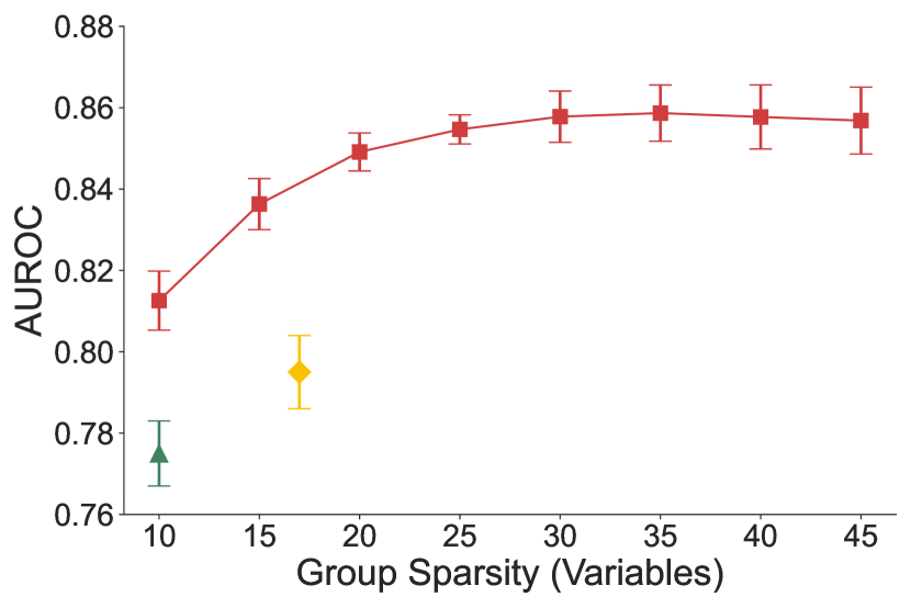
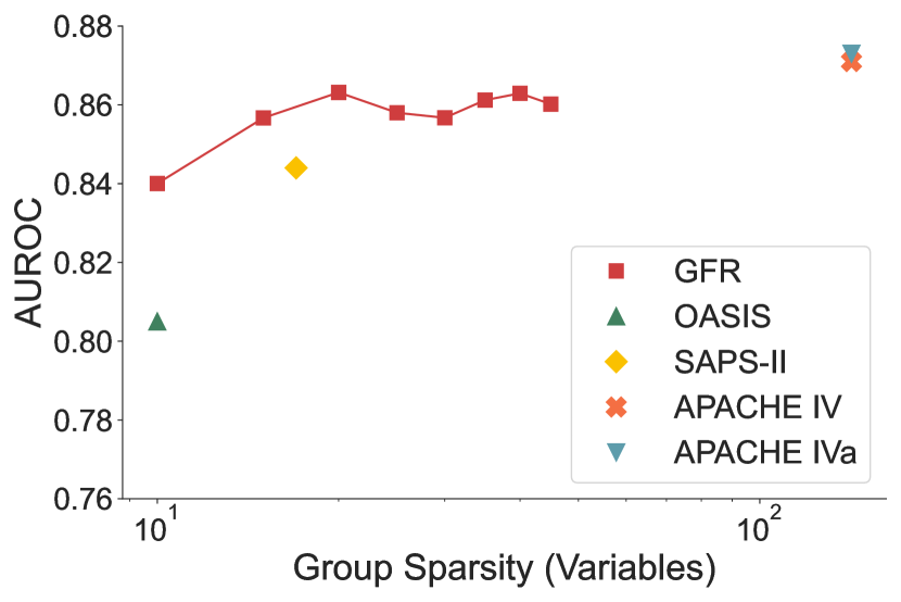
(a)

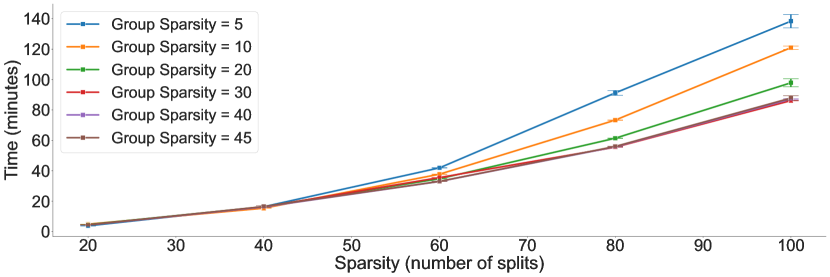
(b) Time consumption to train GroupFasterRisk under various sparsity and group sparsity constraints. Evaluated using five repeated trials on the entire MIMIC III dataset, with sample size of 30,238 and 49 features.

Figure 6: Group sparsities and time consumption of GroupFasterRisk.

Group Sparsity and Runtime: Figure 6(a) shows the predictive accuracy of GroupFasterRisk models under different levels of group sparsity. We find that a higher group sparsity (equivalent to using more features) is positively correlated with an increase in predictive accuracy. However, the increase in AUROC becomes relatively small after 30 variables. It takes at most two hours to train GroupFasterRisk on our MIMIC III cohort (Figure 6(b)) (recall that MIMIC III cohort has 30,238 patients). This is a relatively short amount of time considering that GroupFasterRisk is solving a hard optimization problem, which is NP-hard and combinatorial in nature. We discuss more on our optimization techniques in Section 4.1.

Overall, our results in Figure 4 suggest that GroupFasterRisk is capable of producing robust models that predict in-hospital mortality better or on par as compared to baseline scoring systems, while being more sparse on internal and OOD settings.

2.3 Critical Illness Mortality Prediction for Patients with Sepsis/Septicemia, Acute Kidney Failure, Acute Myocardial Infarction, and Heart Failure

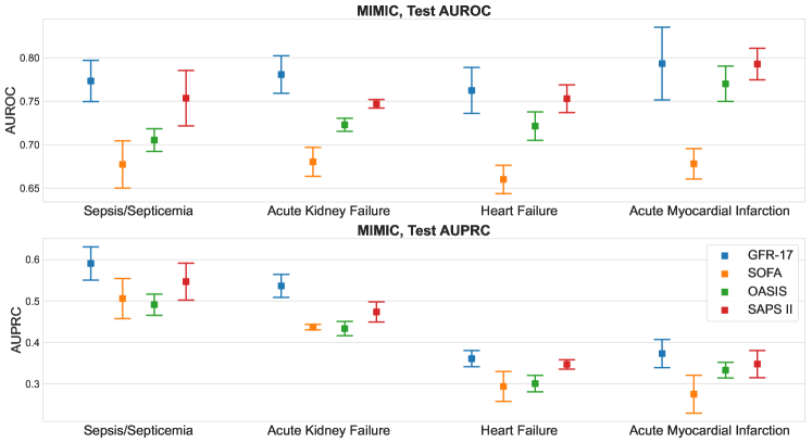
(a)

(a) Results in OOD eICU cohort. GroupFasterRisk is trained on the entire MIMIC III cohort (not on subgroups) using various group sparsity constraints. For each severity of illness score, our GroupFasterRisk models perform on par or better than its baseline while using fewer features.

Sparse Not Sparse GFR-10 OASIS SOFA GFR-15 SAPS II GFR-40 APACHE IV APACHE IVa $F=10$ $F=10$ $F=11$ $F=15$ $F=17$ $F=40$ $F=142$ $F=142$ Sepsis/Septicemia AUROC 0.776 0.734 0.726 0.783 0.782 0.794 0.780 0.781 AUPRC 0.515 0.435 0.461 0.522 0.512 0.549 0.504 0.503 Acute Myocardial Infarction AUROC 0.867 0.846 0.795 0.886 0.879 0.884 0.879 0.886 AUPRC 0.455 0.424 0.395 0.486 0.493 0.521 0.493 0.498 Heart Failure AUROC 0.755 0.731 0.702 0.766 0.770 0.785 0.782 0.787 AUPRC 0.372 0.351 0.337 0.388 0.396 0.425 0.423 0.425 Acute Kidney Failure AUROC 0.774 0.760 0.723 0.801 0.781 0.816 0.803 0.802 AUPRC 0.514 0.472 0.462 0.550 0.527 0.583 0.552 0.550

Figure 7: Evaluation on disease-specific cohorts.

For mortality prognosis tasks, patients with specific critical illnesses are often more prone to risk in ICU [45, 46, 47, 8, 48, 49, 43]. Thus, it is essential to evaluate whether GroupFasterRisk models can provide accurate risk prediction for those population sub-groups. To create disease-specific risk scores, we utilize International Classification of Diseases (ICD) codes in both MIMIC III and eICU to select patients with sepsis or septicemia, acute kidney failure, acute myocardial infarction, and heart failure for our study. We subsequently train GroupFasterRisk models on those sub-populations in the MIMIC III dataset. For simplicity, we refer to patients in those four subgroups as disease-specific cohorts in the rest of this paper. Given that our selected critical illnesses are organ-failure-related, we incorporate SOFA [8] as an additional baseline. While SOFA was initially developed for assessing morbidity, subsequent studies have validated its utility in mortality prediction [50, 51], prompting our decision to include it for comparison.

Figure 7(a) shows an evaluation across all four critical illnesses on internal MIMIC III test folds. GFR-17 achieves higher mean AUROC and AUPRC for all disease-specific cohorts when compared to OASIS, SOFA, and SAPS-II.

Table 2(a) contains our results for OOD evaluation on eICU dataset. Here, we trained on the entire MIMIC III dataset, not on subgroups like we did for Figure 7(a) to be consistent with the other methods (that are used for all subgroups). Our GroupFasterRisk models outperform OASIS and SOFA across all disease-specific cohorts. GFR-40 models outperform APACHE IV/IVa for sepsis, septicemia, and acute kidney failure cohorts. For GFR-15, we observe higher predictive accuracy than SAPS II on both sepsis or septicemia and acute kidney failure cohorts.

Our results highlight the flexibility of GroupFasterRisk, as its models perform well across subgroups, and the method can also be tailored to subgroups if desired.

2.4 GroupFasterRisk Features Are More Informative Than OASIS Features

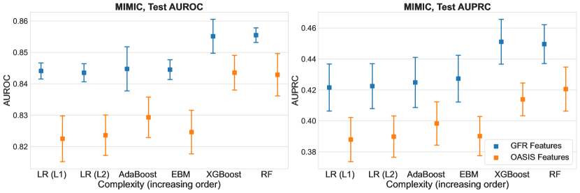
Figure 8: Predictiveness of GroupFasterRisk features against OASIS features. When evaluating the MIMIC III cohort, we find that GFR-14 features empower ML models to perform better than their counterparts when trained on OASIS features.

Since GroupFasterRisk is designed to find solutions for sparse logistic regression, we can alternatively use GroupFasterRisk as a tool for automated, data-driven feature selection. In particular, features selected by GroupFasterRisk should be more informative in predicting the outcome than those features that were not selected. Furthermore, the risk scores reveal how the risks change with each of the feature values.

We now evaluate the ability of GroupFasterRisk to select good features on our internal MIMIC III dataset. To match the number of OASIS variables (see Methods section for details), we selected 14 distinct variables (including all of their thresholds) by training a GFR-14 model and extracting the fourteen features it chose. We then trained black box and interpretable ML models, including Logistic Regression, EBM, Random Forest, AdaBoost, and XGBoost, using features selected by GFR-14. To benchmark our results, we compare with the OASIS+ approach, which demonstrates that ML models trained on OASIS features can obtain high predictive accuracy [18]. Figure 8 shows a comparison of predictive accuracy between GFR-14 and OASIS features. We discover that the vast majority of ML models exhibit enhanced predictive performance when trained on GFR-14 features. More specifically, all models trained on GFR-14 features achieve statistically significantly higher AUROC and AUPRC than those trained on OASIS features ($p<0.01$). Our results demonstrate that GroupFasterRisk naturally selects statistically useful features, enabling the development of ML models that are more predictive than the existing OASIS+ approach.

2.5 GroupFasterRisk Models Are Accurate and Sparse

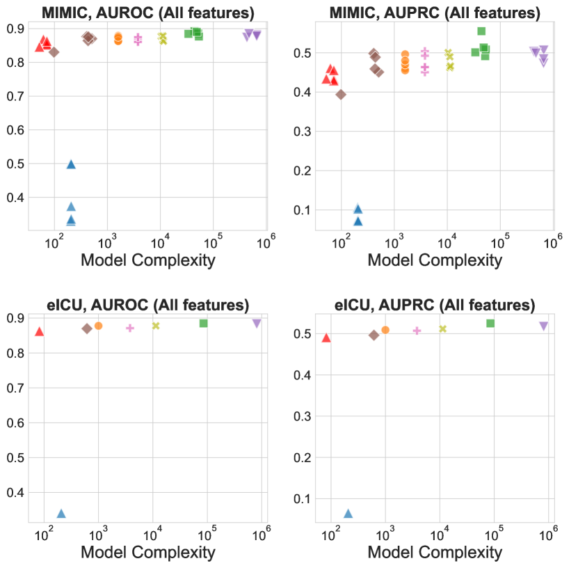
(a) All features.

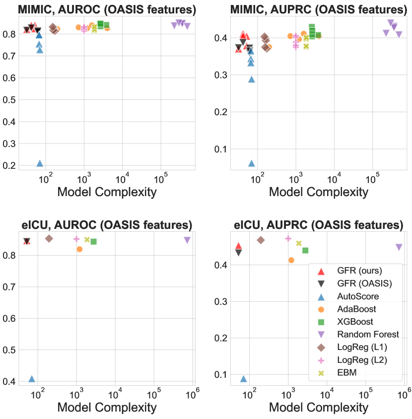
(b) OASIS features.

Figure 9: Performance vs. Complexity

 

As we observed in Figure 4 and Figure 7, GroupFasterRisk models outperform existing severity of illness scores in mortality prediction while being simpler. We further illustrate this point by comparing GroupFasterRisk’s with more complex ML approaches. We will see that GroupFasterRisk is able to perform similarly to black box ML models while being orders of magnitude sparser.

We conduct two experiments to assess the relationship between our methods’ model complexity and AUROC or AUPRC. In the first experiment, we train different ML models using the OASIS features, including Logistic Regression, Random Forest, AdaBoost, EBM, XGBoost, and AutoScore. We compare their performance against our GFR-14 model (using our own features) and GroupFasterRisk trained on OASIS features, namely GFR-OASIS. In the second experiment, we train the same ML models using all 49 features we obtained from the MIMIC III dataset. We compare these models with GFR-40.

We show results based on OASIS features in Figure 9(b) and results based on all features in Figure 9(a). For both setups, we find that GroupFasterRisk models (GFR-14, GFR-40, GFR-OASIS) consistently achieve the best sparsity and high AUROC and AUPRC. Among the different methods we compared with, AutoScore models are the least complex and rely on around 100 parameters, but their performance is substantially worse. Random Forest models achieve the highest AUROC and AUPRC scores, however, these models are very complex and rely on $\sim 10^{6}$ parameters, while GroupFasterRisk models use at most 82 parameters. Other methods such as $\ell_{2}$-regularized Logistic Regression and EBM were as complex as boosted decision trees in terms of the total number of splits across all trees, $\sim 10^{3}$. To sum up, GroupFasterRisk models consistently have high performance while being orders of magnitude sparser than baseline models.

2.6 GroupFasterRisk Produces Reliable and Fair Risk Predictions

In critical care settings, the trustworthiness and fairness of a model’s predictions are paramount since they could considerably affect its usability [52]. To assess the GroupFasterRisk models and the severity of illness score baselines, we use the calibration and predictive accuracy metrics outlined in Section 2.1.1. We consider our eICU cohort for the evaluations because it offers a larger sample size and encompasses multi-center data from across the United States. Subsequently, we evaluate GroupFasterRisk models across various demographic subgroups, considering factors like ethnicity and gender.

Our results are presented in Table 2. We observe that GroupFasterRisk models are not particularly biased towards the majority race (Caucasians) and are well-calibrated on specific subgroups in our eICU cohort. GroupFasterRisk models consistently achieve low Brier scores and HL $\chi^{2}$ across population subgroups. Except in a few cases, GroupFasterRisk models’ Brier scores, HL $\chi^{2}$, and SMR are better than those of OASIS, SAPS II, and APACHE IV/IVa. On average, across all ethnic and gender groups, GFR-10, GFR-15, and GFR-40 achieve SMR of 0.986$\pm$0.041, 1.004$\pm$0.040, and 1.005$\pm$0.058, respectively, which are all close to 1 (the best possible value). Among sparse models (no more than 17 variables), GroupFasterRisk achieves the highest AUROC and AUPRC across subgroups. We present additional ROC, PR, and calibration curves in Section C.3.

Table 2: Fairness and calibration across population subgroups in eICU.

Ethnicity (alphabetical order) Gender African American Asian Caucasian Hispanic Native American Other/Unknown Female Male Percentage ($\%$) 11.17 1.49 76.91 3.86 0.68 4.68 45.08 54.90 AUROC ($\uparrow$) GFR-10 0.829 0.833 0.837 0.856 0.881 0.849 0.835 0.840 OASIS 0.811 0.797 0.803 0.825 0.824 0.809 0.806 0.805 GFR-15 0.846 0.848 0.854 0.873 0.895 0.860 0.853 0.856 SAPS II 0.846 0.828 0.843 0.859 0.893 0.842 0.844 0.845 GFR-40 0.859 0.861 0.859 0.881 0.902 0.873 0.857 0.865 APACHE IV 0.873 0.858 0.869 0.890 0.903 0.884 0.867 0.875 APACHE IVa 0.875 0.866 0.870 0.893 0.901 0.886 0.869 0.876 AUPRC ($\uparrow$) GFR-10 0.415 0.390 0.422 0.480 0.558 0.418 0.418 0.429 OASIS 0.345 0.330 0.364 0.410 0.370 0.328 0.356 0.365 GFR-15 0.453 0.454 0.466 0.534 0.555 0.477 0.466 0.471 SAPS II 0.424 0.408 0.435 0.470 0.598 0.395 0.440 0.428 GFR-40 0.488 0.500 0.489 0.553 0.585 0.512 0.488 0.499 APACHE IV 0.488 0.467 0.484 0.536 0.536 0.479 0.478 0.493 APACHE IVa 0.487 0.492 0.487 0.538 0.522 0.484 0.481 0.496 Brier Score ($\downarrow$) GFR-10 0.064 0.070 0.068 0.065 0.059 0.065 0.068 0.067 OASIS 0.068 0.076 0.072 0.068 0.072 0.070 0.072 0.070 GFR-15 0.062 0.068 0.065 0.061 0.059 0.061 0.065 0.064 SAPS II 0.080 0.080 0.082 0.074 0.072 0.078 0.080 0.081 GFR-40 0.060 0.064 0.064 0.060 0.057 0.059 0.064 0.062 APACHE IV 0.063 0.069 0.066 0.062 0.066 0.064 0.066 0.064 APACHE IVa 0.061 0.065 0.064 0.060 0.062 0.061 0.064 0.062 HL $\chi^{2}$ ($\downarrow$) GFR-10 27.90 11.00 113.70 24.68 5.48 12.53 58.65 102.74 OASIS 43.48 21.02 135.52 5.23 14.84 11.75 82.52 79.11 GFR-15 23.64 9.88 63.40 10.62 4.43 3.73 13.62 57.75 SAPS II 1070.09 94.34 6599.71 228.75 62.95 333.65 3575.48 4750.90 GFR-40 8.72 5.20 120.03 12.03 11.57 6.09 58.34 97.92 APACHE IV 308.51 34.51 1257.11 78.93 42.53 114.22 835.14 950.18 APACHE IVa 167.60 13.04 502.27 42.78 23.21 62.48 372.68 384.89 SMR ($\sim 1$) GFR-10 0.946 0.915 1.028 1.017 0.949 1.013 0.993 1.031 OASIS 0.882 1.204 0.922 0.994 0.844 1.002 0.917 0.940 GFR-15 0.974 0.921 1.040 1.046 1.003 0.996 1.002 1.046 SAPS II 0.501 0.570 0.517 0.560 0.513 0.552 0.525 0.517 GFR-40 1.022 0.936 1.039 1.063 0.889 1.033 1.000 1.058 APACHE IV 0.663 0.732 0.731 0.710 0.606 0.697 0.716 0.725 APACHE IVa 0.730 0.820 0.823 0.784 0.704 0.778 0.802 0.815

3 Discussion

Table 3: Comparison of GroupFasterRisk with other current mortality prediction methods.
*We consider the following Severity of Illness Scores: OASIS, SOFA, SAPS II, and APACHE IV/IVa

GroupFasterRisk Severity of Illness Scores* Black-box ML AutoScore Interpretable models? ✓ ✓ ✗ ✓ Can be trained on specific subpopulations? ✓ ✗ ✓ ✓ Allow post-correction to suit domain knowledge. ✓ ✗ ✗ ✓ Automatically produce risk cards? ✓ ✗ ✗ ✓ Allow feature extraction? ✓ ✓ ✗ ✓ Allow hard constraints in optimization? ✓ ✗ ✗ ✓ High predictive accuracy? ✓ ✓ ✓ ✗

Our work introduces GroupFasterRisk, an ML algorithm capable of creating a diverse set of accurate severity of illness scores while being highly flexible. We demonstrate that our approach generally outperforms existing severity of illness scores, is capable of selecting highly predictive variables, and performs well on population sub-groups based on race and gender in terms of robustness, accuracy, fairness, and calibration. Moreover, our models perform similarly to black-box ML models learned on the same data while being orders or magnitude sparser and simpler. Our framework provides an accessible and fast procedure to learn an interpretable model from data and could be used to support medical practitioners in the development of severity of illness scores and beyond. There are multiple aspects of our study worthy of discussion; we firstly focus on the advantages of GroupFasterRisk (summarized in Table 3) and then on the limitations of our study.

Interpretability: GroupFasterRisk generates scorecard displays (such as the one in Figure 1). From those displays, one can quickly evaluate the correctness of the model and make adjustments if desired. For instance, the feature component scores, shown as the rows in Figure 1, allow medical practitioners to interpret the relationship between risk (value of the integers) and the possible values of the features. Additionally, the group sparsity constraint $\gamma$ enforces the selection of, at most, the top $\gamma$ useful features, informing the user about the meaningful variables in the prediction-making process. Combined together, this score calculation process from GroupFasterRisk models is transparent and interpretable to the user at any level of medical expertise. This could be beneficial for healthcare applications in several ways: (1) It enables users to directly see the model itself and every single step of its prediction-making process, supporting the discovery of new knowledge or potential bias in the model without the need for post-hoc explanations. (2) If the model does not suit medical knowledge due to empirical noise in data, practitioners could further adopt monotonicity corrections to adjust the model. (3) The diverse pool of solutions provides users with a set of equally accurate risk scorecards, which helps to resolve the “interaction bottleneck” between people and algorithms. Users can choose among numerous available models to pick one that aligns the best with medical knowledge. These advantages can largely support health professionals in practice compared with black box ML models. (4) Our code includes the option of monotonicity constraints for interpretability. This allows, for instance, the user to constrain the risk scores to increase with age. To evaluate whether monotonicity correction can aid the development of more predictive models, we provide ablation studies in Section C.1. We find that models corrected with monotonicity constraints demonstrate increased predictive accuracy in OOD evaluations compared to the original, uncorrected models. This suggests that incorporating domain-relevant knowledge into risk score design could further enhance performance.

Sparsity: Among the different scoring systems we compared in the paper, APACHE IV/IVa is among the most accurate. Both APACHE IV/IVa rely on 142 features for a completed setup of patient risk predictions. In comparison, our most complex model GFR-40 achieves similar performances as APACHE IV/IVa while requiring only 40 features for its risk prediction process. In practice, this 3.5 times difference in the number of features can be quite significant, especially when accounted for missing values or other collection errors that commonly occur in medical data [53]. While there are several ways to handle missing data, such as treating missing values as 0 or using other statistical imputation techniques [54, 55], these methods can negatively affect prediction accuracy, limit performance guarantees, and create an extra task for medical practitioners to complete in practice. Since GFR-40 expects 40 features for its risk prognosis prediction, it is less likely to require practitioners to address missing value problems as compared to APACHE IV/IVa. Furthermore, compared to other ML approaches, GroupFasterRisk models are 1,000 times sparser in model complexity while achieving comparable performance. Since studies have shown that humans can at most manage 7$\pm$2 cognitive entities at the same time [56, 57], the sparse-learning nature of GroupFasterRisk can be supportive for medical practitioners since it is the basis for creating interpretable models.

Flexibility: Most existing severity of illness scores are fixed and provided as they are, making it difficult to adjust them to suit different populations. They are also not applicable to re-train and cannot be adapted for specific subpopulations. Moreover, they can be time- and resource- costly to construct and learn in the first place. For example, SAPS II was constructed from expert knowledge, and OASIS was created via a semi-manual process involving feature selection and fine-tuning of coefficients. By contrast, GroupFasterRisk is a data-driven ML algorithm capable of adapting to different datasets and producing risk scores tailored to any population in a reasonable amount of time. Rather than a fixed risk score, we provide a flexible system to compute numerous risk scores. Practitioners can set arbitrary grouping of the features, sparsity, and box constraints to design risk scores of their choice. They can learn a scoring system for a specific cohort of interest or different datasets. They can adjust risk scores manually if desired, using the approach of [58]. Further, as we discussed before, GroupFasterRisk can provide more than one high-performing solution as discussed in Figure 2. In this case, experts can choose a solution that they prefer and adopt a risk score that best suits their needs. GroupFasterRisk selects important features for prediction, which we have experimentally demonstrated in Figure 8. Lastly, although practitioners still need to determine GroupFasterRisk’s hyperparameters, they are fast to optimize. GroupFasterRisk is capable of creating risk scores within hours on a personal laptop (Apple MacBook Pro, M2).

Generalization: When models are applied across different high-risk settings, it is important that the model generalizes well. Our OOD evaluation is performed on the eICU, a dataset collected from other medical centers independent of our internal dataset MIMIC III. Therefore, we provide an estimate of generalization error by taking into consideration: (1) differences in practice between health systems, (2) variations in patient demographics, genotypes, and phenotypes, and (3) variations in hardware and software for data capture. All of these are important to the generalizability of models in healthcare systems [59]. Our OOD evaluation demonstrates that GroupFasterRisk can generalize well when trained on MIMIC III and tested on eICU for all-cause and disease-specific cohorts.

There are some limitations in how we evaluate the generalizability of GroupFasterRisk models. For instance, changes in patterns over time are still not fully measured. We discuss this issue in Limitation I and II.

Limitation I — Distributional Shifts: Due to data access issues, we could only conduct experiments on MIMIC III and eICU datasets and therefore, our results are limited to the setting of these study cohorts (however, as far as we are aware, these are the largest and most detailed publicly available datasets that have ever existed on ICU monitoring.). MIMIC III and eICU were collected between 2001-2012 and 2014-2015, respectively, which limits us from performing further evaluation on samples collected from the current period. For future research, it is worth investigating whether the results and conclusion still hold on samples from a different time period. Furthermore, changes in population distribution due to temporal drift have been shown to impact model predictive accuracy [60]. However, due to the de-identification process in both MIMIC III and eICU that keeps the admission date private, we are unable to perform such an evaluation. Second, both MIMIC III and eICU are datasets collected from hospitals in the United States. This limits the scope of our work in other countries, and thus our results may not be directly applicable to other geographical locations. Nonetheless, we believe further evaluations using data collected from different countries and a more recent time period could address these limitations. Our methods may be substantially faster in generating risk scores in different geographical areas and time periods than the considered baselines and competitors, since GroupFasterRisk constructs models automatically, rather than manually.

Limitation II — Data Collection Process: Given the retrospective nature of our study, there are inherent limitations related to how MIMIC III and eICU collect data, especially for time series measurements. For instance, vital signs in eICU are first recorded as one-minute averages and then stored as five-minute medians, implying our data may not perfectly represent true vital sign measurements in practice. Although our study does not involve the direct use of time series measurements in patient records, we use summary statistics that may still be affected by changes in measurement processing or aggregation.

Additionally, to have more access to the measurements of the patients, our MIMIC III cohort considers patients who stayed in the ICU for more than 24 hours (see Section A.1). Such design could cause bias in our models in predicting mortality for patients admitted to the ICU for less than one day. Thus, to provide a more comprehensive evaluation, our eICU cohort relaxes this restriction by including all patients who have been admitted for more than 4 hours. This criteria is also more consistent with the study cohort used to create OASIS and APACHE IV and allows a more rigorous evaluation of GroupFasterRisk models. Our results in the previous section fully support that GroupFasterRisk performs well under these shifted hours of ICU stay.

Limitation III — APACHE IV/IVa in Internal Setting: Another limitation of our study is that we cannot compute APACHE IV/IVa scores on the MIMIC III dataset (due to the lack of information for admission diagnosis in MIMIC III). Again, APACHE IV/IVa requires 142 features, which provides a disadvantage to evaluation and practical use.

4 Methods

4.1 Finding High-quality Solutions with GroupFasterRisk

Define a dataset as $\mathcal{D}=\{1,\bm{\tilde{x}}_{i},y_{i}\}_{i=1}^{n}$, where $y_{i}\in\{0,1\}$ is a label, $\bm{\tilde{x}}_{i}\in\mathbb{R}^{p}$ is a binarized feature vector (see Section 4.3 for details), $\bm{x}_{i}\in\mathbb{R}^{q}$ is the raw feature vector, and $1$ is added for ease of notation and represents an intercept. The set of feature indices $\{1,...,p\}$is arbitrarily partitioned into $\Gamma$ disjoint sets (groups), denoted as $\{G_{k}\}_{k=1}^{\Gamma}$. Let $\mathcal{D}/m=\left\{1/m,\bm{\tilde{x}}_{i}/m,y_{i}\right\}_{i=1}^{n}$ be a scaled dataset, where we scale by a multiplier $m$, $m>0$ ($m$ will be learned by the algorithm). Let our hypothesis space be a space of linear models $\bm{w}^{\top}\bm{\tilde{x}}+w_{0}$, where $\bm{w}\in\mathbb{R}^{p}$ and $w_{0}\in\mathbb{R}$. We denote $\bm{w}_{G_{k}}\in\mathbb{Z}^{|G_{k}|}$ as entries in $\bm{w}$ that belong to a group $G_{k}$.

Our goal is to obtain integer-valued solutions of a sparse ($\ell_{0}$ regularized) logistic regression problem under sparsity, group sparsity, and box constraints, denoted as $\lambda$, $\gamma$, $\left({\bm{a}},{\bm{b}}\right)$, respectively, where ${\bm{a}},{\bm{b}}\in\mathbb{R}^{p}$, $w_{j}\in[a_{j},b_{j}]$ for all $j$. We denote a solution as $(\bm{w},w_{0})$ and outline the purpose of each hyperparameter below.

Sparsity: The sparsity constraint $\lambda$ is the number of non-zero elements in the solution vector ${\bm{w}}$ and directly controls the model complexity in the risk scorecards. The users can directly set $\lambda$, and GroupFasterRisk produces a diverse pool of solutions that strictly satisfies this hard constraint. Intuitively, when GroupFasterRisk is trained on binarized data, $\lambda$ corresponds to the number of binary stumps or decision splits in the final model(s).

Group Sparsity: Group sparsity constraint $\gamma$ allows users to control the number of partitions on the features in the final solution. In most cases and throughout all our experiments, binary stumps belonging to a single feature could be treated as a group. Under this treatment of groups, using group sparsity of $\gamma$ is equivalent to optimizing the risk score using at most $\gamma$ features, allowing the creation of more cohesive models for users to interpret. Alternatively, medical practitioners could also define groups based on similarity between features using their domain knowledge, such as grouping height and weight together since they are both biometric attributes, creating risk scores that best suit their needs.

Box Constraint: Box constraint $\left({\bm{a}},{\bm{b}}\right)$ is also defined by the user and allows users to limit the solution values to their desired range, i.e., $w_{j}\in[a_{j},b_{j}]$. This hyperparameter allows users to control the range of the coefficients on their final risk scores, providing more control over the final solution(s).

Overall, the problem of computing an integer-valued linear model is NP-hard. However, we solved it by finding a good approximate solution and using $m$ as a multiplier to do so. While $\left(\bm{w},w_{0}\right)$ must be integer-valued, the product $\left(\bm{w}^{\top}\bm{\tilde{x}}/m+w_{0}/m\right)$ can be real-valued. Intuitively, division by a range of multipliers extends through the solution space like the rays of a star, and a subroutine is adopted to determine the multiplier.

We formulate the problem of creating risk scores as an optimization problem in Equation 1. More specifically, we optimize logistic loss in Equation 1a for real-valued solution $\left(\bm{w}^{\top}\bm{\tilde{x}}/m+w_{0}/m\right)$, with sparsity constraint $\lambda$ and integer constraint (Equation 1b), box constraint $\left({\bm{a}},{\bm{b}}\right)$ (Equation 1c), group sparsity constraint $\gamma$ (Equation 1e), and multiplier $m$ (Equation 1d), where $\mathbb{I}\{\cdot\}$ denotes the indicator function.

$$\min_{\bm{w},w_{0},m}\mathcal{L}(\bm{w},w_{0},\mathcal{D}/m)=\sum_{i=1}^{n}\log\left(1+\exp\left(-y_{i}\frac{\bm{w}^{\top}\bm{\tilde{x}}_{i}+w_{0}}{m}\right)\right)\\$$ (1a)

s.t. $$\|\bm{w}\|_{0}\leq\lambda,\bm{w}\in\mathbb{Z}^{p},w_{0}\in\mathbb{Z}\quad\textit{\color[rgb]{0,0.51171875,0}{\# at most $\lambda$ integer coefficients}}$$ (1b)

$$w_{j}\in[a_{j},b_{j}]\quad\forall j\in\{1,...,p\}\quad\textit{\color[rgb]{0,0.51171875,0}{\# control range of coefficients}}$$ (1c)

$$m>0\quad\textit{\color[rgb]{0,0.51171875,0}{\# expand solution space using multiplier}}$$ (1d)

$$\sum_{k=1}^{\Gamma}\mathbb{I}\left\{\bm{w}_{G_{k}}\neq\bm{0}\right\}\leq\gamma.\quad\textit{\color[rgb]{0,0.51171875,0}{\# at most $\gamma$ groups, where $G_{k}$ are the indices of group $k$}}$$ (1e)

We solve the optimization problem in Equation 1 similarly to [29] in three steps (as in Figure 2):

1. We first relax the integer value constraints and find a real-valued solution $(\bm{w}^{(*)},w_{0}^{(*)})$ to sparse logistic regression under box constraint $\left({\bm{a}},{\bm{b}}\right)$.

2. Based on $(\bm{w}^{(*)},w_{0}^{(*)})$, we swap one feature at a time to obtain a set of $M$ sparse diverse real-valued solutions. We use an iterative subroutine to select the features, each of which must strictly satisfy the group constraint $\gamma$. We call this set Diverse Pool and denote the set by $\{(\bm{w}^{(t)},w_{0}^{(t)})\}_{t=1}^{M}$. Diverse Pool’s solutions are nearly as accurate as our original solution $(\bm{w}^{(*)},w_{0}^{(*)})$.

3. For every solution in the Diverse Pool $\{(\bm{w}^{(t)},w_{0}^{(t)})\}_{t=1}^{M}$, we round all the continuous solutions to integers, thus assigning weights to the selected variables and producing a set of risk scores. Unlike direct rounding that could worsen solution quality, we specifically use a subroutine that adapts multiplier $m$ to extend the solution space when rounding the coefficients. A theoretical upper bound on the rounding error is proven in [29]; this choice permits us to maintain a high level of accuracy while rounding.

Together, the three steps allow GroupFasterRisk to produce multiple diverse sparse risk scores with high accuracy. Finally, for a given solution $(\bm{w},w_{0})$, we compute risk predictions as $P\left(Y=1\mid\bm{\tilde{x}}\right)=\sigma\left(\left(\bm{w}^{\top}\bm{\tilde{x}}+w_{0}\right)/m\right)$, where $\sigma(\xi)=1/\left(1+e^{-\xi}\right)$ is a sigmoid function.

4.2 Feature Selection and Engineering

Our feature selection process was divided into two stages. First, we created a set of features by taking the union of features used by existing severity of illness scores. Specifically, we consider features from Acute Physiology Score III (APS III) [61], Simplified Acute Physiology Score II (SAPS II) [42], Oxford Acute Severity of Illness Score (OASIS) [14], Sequential Organ Failure Assessment (SOFA) [8], Logistic Organ Dysfunction Score (LODS) [62], and Systemic Inflammatory Response Syndrome criteria (SIRS) [63]. Second, we computed the receiver operating characteristic curve (ROC) and the corresponding area under the curve (AUC) value for every feature individually. By analyzing AUC and the shape of ROC curves, we estimate the predictive ability of every feature on in-hospital mortality for all the patients in the MIMIC III training set. This provides us with a ranking of all features, and we selected the top 49 features for this study.

To include time series measurements such as vital signs, we extracted the minimum and maximum of these features during the first 24 hours of a patient’s unit stay. This allows us to focus on the worst deviation from a normal range of values. Minimum and maximum values of time series data are often easier to observe by medical practitioners than other more sophisticated statistics (such as variance), making them convenient from a practical point of view. Additionally, most existing severity of illness scores also rely on the worst values over a time period.

4.3 Feature Binarization

We transformed every continuous or categorical feature into a set of binary decision splits. This allows GroupFasterRisk to capture a non-linear step function for each feature when it learns coefficients for those decision splits. For continuous variables, a step function on feature $l$ at threshold $\theta_{l,\tilde{l}}$ would be denoted $\mathbb{I}\{x_{l}\leq\theta_{l,\tilde{l}}\}$, which is 1 if $x_{l}\leq\theta_{l,\tilde{l}}$ and 0 otherwise. The component function for feature $l$ would then sum up the step functions for all the thresholds and would be denoted $f_{l}(x_{l})=\sum_{\tilde{l}\in G_{l}}w_{\tilde{l}}\mathbb{I}\{x_{l}\leq\theta_{l,\tilde{l}}\}$. The full model $f(\bm{x})$ would be the sum of the component functions, $\sum_{l}f_{l}(x_{l})$. We used two methods to create the splits $\theta_{l,\tilde{l}}$: 1) For binary or categorical features, a split was created between each pair of unique feature values for each feature. 2) We obtained the distribution of feature values based on the training data and computed quantiles of the distributions and used them as decision splits. (Alternatively, the splits can be set as a hyperparameter.) This preprocessing procedure makes GroupFasterRisk models generalized additive models (GAMs), which have been demonstrated to be as accurate as any black box ML model for most tabular data problems [64, 65, 33].

4.4 GroupFasterRisk Monotonic Correction

GroupFasterRisk provides the option of a monotonic correction so that the risk score is forced to increase (or decrease) along a variable. This allows users to better align the modeling process with domain knowledge. More specifically, GroupFasterRisk allows users to set box constraints $(\bm{a}_{G_{l}},\bm{b}_{G_{l}})$ for each feature $l$ independently (recall that we set each group as the decision splits belonging to each feature). These constraints can be imposed after any of the three GroupFasterRisk optimization steps. Because of the binarization preprocessing step, each feature corresponds to a set of step functions. Imposing monotonicity is equivalent to forcing all coefficients for all step functions of one feature to be positive (for decreasing functions) or negative (for increasing functions). If $\bm{a}_{G_{l}},\bm{b}_{G_{l}}\geq\bm{0}$, then $f_{l}(x_{l})$ is monotonically decreasing; if $\bm{a}_{G_{l}},\bm{b}_{G_{l}}\leq\bm{0}$, then component function $f_{l}$ is monotonically increasing.

Our risk score in Figure 1 has been applied with monotonicity correction. Particularly, we set the box constraint for Max Bilirubin and Max BUN to be between $[-100,0]$ and Min GCS and Min SBP to be between $[0,100]$. This helps to prevent the algorithm from overfitting the model to noise in the data. For instance, without monotonicity constraints, we observed that the component function for Min GCS was non-monotonic at extreme values. This model would imply that patients with GCS of 3 are less risky than those with GCS of 6, which (while a realistic reflection of the information contained in the training data) is not aligned with medical knowledge. Our monotonicity correction prevents this from happening.

4.5 Training and Evaluation of GroupFasterRisk and ML Baselines

We trained GroupFasterRisk models with various group sparsity constraints between 10 and 45. For each group sparsity, we performed hyperparameter optimization using grid search and Bayesian optimization to determine the optimal hyperparameter. We ran two sets of experiments to evaluate GroupFasterRisk.

First, we used 5-fold nested cross-validation to evaluate performance on MIMIC III, i.e., we performed hyperparameter optimization on the training fold for each train/test split and used the best hyperparameter on the test set for evaluation.

Our second set of experiments evaluates the performance out of sample on the eICU dataset. We trained our models and performed hyperparameter optimization on the MIMIC III dataset, and evaluated them on the eICU cohort.

We used the same training and evaluation procedures for the ML baselines. The hyperparameters used in this study are contained in our code repository.

4.6 Severity of Illness Scores Evaluation

We benchmarked the performance of GroupFasterRisk against established severity of illness scores on MIMIC III and eICU study cohorts. For MIMIC III, we implemented the risk score calculation made by MIT-LCP. In particular, we calculated OASIS, SOFA, and SAPS-II for in-hospital mortality risk prediction and evaluated their performance on the same 5 test folds as GroupFasterRisk. We also attempted to calculate APACHE IV/IVa score on MIMIC III, but we ran into difficulty because the reason of admission variable was difficult to obtain. Although such information could potentially be inferred using natural language processing on the Noteevents table [30], this inference procedure has not been verified to reliably extract factually correct information, so we did no compute APACHE IV/IVa on MIMIC III.

For OOD evaluation on eICU, we referenced the OASIS calculation using the official code repository and calculated SAPS-II and SOFA scores from their published formulas. APACHE IV/IVa in-hospital mortality predictions are directly contained within the eICU dataset. We evaluated all severity of illness score baselines on the same study cohort as GroupFasterRisk.

4.7 Fairness and Calibration Evaluations

We used the eICU dataset for fairness evaluation since it has a multi-center data source collected from the entire United States. It has the advantage of containing more samples for each subgroup than MIMIC III. We separated the subgroups from the eICU study cohort by race and gender. For GroupFasterRisk, AUROC and AUPRC were computed for each subgroup using models trained on the entire MIMIC III cohort. In other words, GroupFasterRisk models were trained on the entire training population, without fitting to specific populations, and evaluated on the subgroups in the OOD setting. For severity of illness score baselines, we calculated AUROC and AUPRC directly on every eICU subgroup.

We calibrated GroupFasterRisk using isotonic regression on a subset of 2,000 patients drawn randomly from our eICU cohort, equivalent to about 1.84$\%$ of the entire cohort. We also provided the comparative experiment where we calibrate severity of illness score baselines in Section C.3; the results did not change.

5 Data Availability

Medical Information Mart for Intensive Care III Database (MIMIC-III) and eICU Collaborative Research Database (eICU or eICU-CRD)[30, 31] are both publicity available at https://mimic.mit.edu/ and https://eicu-crd.mit.edu/, respectively. Access to the datasets require CITI Data or Specimens Only Research certifications and signing corresponding data use agreements, as well as institutional IRB approval at Duke.

6 Code Availability

The software developed in this study is available at https://github.com/jiachangliu/FasterRisk. The source code for experiments involved in this study is available at https://github.com/MuhangTian/GFR-Experiments.

Appendix to “Fast and Interpretable Mortality Risk Scores for Critical Care Patients”

Appendix A Experiment Details

A.1 Study Population

Figure 10: Flow chart of the study population selection on MIMIC III and eICU-CRD database. $i$ and $n$ are ICU stays and number of patients, respectively.

MIMIC-III

MIMIC-III is a large, single-center database comprised of health-related information of 53,423 hospital admissions for adult patients (aged 16 years or above) admitted to critical care units of the Beth Israel Deaconess Medical Center in Boston, MA, between 2001 and 2012. MIMIC-III integrates de-identified, comprehensive clinical data of 38,597 distinct adult patients. It includes patient information such as laboratory measurements, vital signs, notes charted by healthcare providers, diagnostic codes, hospital length of stay, and survival data. Besides mortality prediction, MIMIC-III has been used by academic and industrial research to investigate novel clinical relationships and develop new algorithms for patient monitoring [30].

eICU

The eICU Collaborative Research Database, sourced from the eICU Telehealth Program, is a multi-center ICU database with high granularity data containing 200,859 admissions to ICUs monitored by eICU programs across the United States. The database includes 139,367 unique patients admitted to critical care units in 2014 and 2015. Built upon the success of MIMIC-III, eICU includes patients from multiple medical centers. The source hospital of MIMIC-III does not participate in the eICU program, which makes eICU a completely independent set of healthcare data suitable for out-of-distribution evaluation [31].

A.2 Severity of Illness Score Implementations

We observe a discrepancy between official implementations of OASIS and SAPS II in the MIMIC III code repository with their respective original works. In particular, the calculation of the sub-score for pre-ICU length of stay differs from that published in the original paper [14], and the implementation for bicarbonate sub-score in SAPS II also differs from the original work in [42]. Details of the implementation errors can be found in this GitHub issue. We corrected those mistakes in our implementations for OASIS and SAPS II and detailed the effects caused by our corrections in Table 4.

The APACHE IV/IVa scores are directly contained in the eICU dataset [31], thus, there was no need to implement these scores ourselves.

Table 4: Effect of implementation correction for OASIS and SAPS II.

		OASIS Correction	SAPS II Correction
MIMIC III	Affected Patients ($\%$) a	22.93	4.38
	AUROC Change	+0.001	0.000
	AUPRC Change	-0.001	+0.001
	HL $\chi^{2}$ Change	+18.59	+17.06
	Brier Score Change	+0.001	0.000
	SMR Change	-0.011	-0.002
eICU	Affected Patients ($\%$)	14.07	6.09
	AUROC Change	+0.002	0.000
	AUPRC Change	+0.001	+0.001
	HL $\chi^{2}$ Change	+13.77	+206.87
	Brier Score Change	0.000	0.000
	SMR Change	-0.012	-0.002

Appendix B GroupFasterRisk Algorithm

B.1 Optimization Procedures Outline

We use the same notation as Section 4.1. To solve the optimization problem in Equation 1, we solve three consecutive optimization sub-problems. In the first step, Equation 2, we approximately find a near-optimal solution for sparse logistic regression sparsity and box constraints, denoted as $\lambda$ and $({\bm{a}},{\bm{b}})$, respectively.

$$\begin{split}(\bm{w}^{(*)},w_{0}^{(*)})\in\operatorname*{arg\,min}_{\bm{w},w_{0}}\mathcal{L}\left(\bm{w},w_{0},\mathcal{D}\right)&=\sum_{i=1}^{n}\log\left(1+\exp\left(-y_{i}\left(\tilde{\bm{x}}_{i}^{\top}\bm{w}+w_{0}\right)\right)\right)\\ \textrm{s.t. }&\|\bm{w}\|_{0}\leq\lambda,\bm{w}\in\mathbb{R}^{p},w_{0}\in\mathbb{R}\\ &\forall j\in[p],w_{j}\in[a_{j},b_{j}]\\ &\sum_{k=1}^{\Gamma}\mathbb{I}\left\{\bm{w}_{G_{k}}\neq\bm{0}\right\}\leq\gamma.\end{split}$$ (2)

Solving Equation 2 produces an accurate and sparse real-valued solution $(\bm{w}^{(*)},w_{0}^{(*)})$ that satisfies both feature and group sparsity constraints.

In the second step, we aim to produce multiple real-valued near-optimal sparse logistic regression solutions under group sparsity constraint, which is formulated as:

$$\begin{split}(\bm{w}^{(t)},w_{0}^{(t)})\text{ obeys }&\mathcal{L}(\bm{w}^{(t)},w_{0}^{(t)},\mathcal{D})\leq\mathcal{L}(\bm{w}^{(*)},w_{0}^{(*)},\mathcal{D})(1+\epsilon_{u})\\ \textrm{s.t. }&\|\bm{w}^{(t)}\|_{0}\leq\lambda,\bm{w}^{(t)}\in\mathbb{R}^{p},w_{0}^{(t)}\in\mathbb{R}\\ &\forall j\in[p],w_{j}^{(t)}\in[a_{j},b_{j}]\\ &\sum_{k=1}^{\Gamma}\mathbb{I}\left\{\bm{w}^{(t)}_{G_{k}}\neq\bm{0}\right\}\leq\gamma.\end{split}$$ (3)

In particular, in order to solve Equation 3, we delete a feature $j_{-}$ with support in $supp(\bm{w}^{(*)})$ and add a new feature with index $j_{+}$. This procedure is repeated to turn the solution $(\bm{w}^{(*)},w_{0})$ into diverse sparse solutions with similar logistic loss. Note that during swapping, we only consider the alternative features that obey various constraints (including box constraint, groups-sparsity constraint, and monotonicity constraint) to ensure the new solutions are valid models.

$$\text{Find all $j_{+}$ s.t.}\min_{\delta\in[a_{j_{+}},b_{j_{+}}]}\mathcal{L}(\bm{w}^{(*)}-w^{(*)}_{j_{-}}\bm{e}_{j_{-}}+\delta\bm{e}_{j_{+}},w_{0},\mathcal{D})\leq\mathcal{L}(\bm{w}^{(*)},w_{0}^{(*)},\mathcal{D})\left(1+\epsilon_{u}\right).$$ (4)

We solve Equation 3 several times (set by the user as a hyper-parameter), after which we have a pool of distinct, almost-optimal sparse logistic regression models, and the top $M$ models with the smallest logistic loss are selected, creating $M$ solutions $\{(\bm{w}^{(t)},w_{0}^{(t)})\}_{t=1}^{M}$. Note that the user can set $\epsilon_{u}$ and $M$ arbitrarily, controlling the tolerance in logistic loss and the desired maximum quantity of diverse sparse solutions.

Lastly, for each solution in $\{(\bm{w}^{(t)},w_{0}^{(t)})\}_{t=1}^{M}$, we compute an integer risk score, $(\bm{w}^{(+t)},w_{0}^{(+t)})$, by performing rounding to a real-valued solution:

$$\begin{split}\mathcal{L}\left(\bm{w}^{(+t)},w_{0}^{(+t)},\mathcal{D}/m^{(t)}\right)&\leq\mathcal{L}\left(\bm{w}^{(t)},w_{0}^{(t)},\mathcal{D}\right)+\epsilon_{t}\\ \textrm{s.t. }&\bm{w}^{(+t)}\in\mathbb{Z}^{p},w_{0}^{(+t)}\in\mathbb{Z}\\ &\forall j\in[p],w_{j}^{(+t)}\in[a_{j},b_{j}]\\ &\sum_{k=1}^{\Gamma}\mathbb{I}\left\{\bm{w}^{(+t)}_{G_{k}}\neq\bm{0}\right\}\leq\gamma.\\ \end{split}$$ (5)

where $\epsilon_{t}$ is a gap in logistic loss with the near-optimal solution due to rounding. A theoretical upper bound on $\epsilon_{t}$ was proven in [29]. In order to round the coefficients, we perform the following steps: 1) we define the largest multiplier $m_{\text{max}}$ as $\max\{\|{\bm{a}}\|_{\infty},\|{\bm{b}}\|_{\infty}\}/\|{\bm{w}}^{(*)}\|_{\infty}$, and the smallest multiplier $m_{\text{min}}$ to be 1. 2) we select $N_{m}$ equally spaced values within the range $[m_{\text{min}},m_{\text{max}}]$, giving us a set of multipliers. 3) Using this set of multipliers, we scale the dataset, obtaining $\left\{1/m,\bm{\tilde{x}}_{i}/m,y_{i}\right\}_{i=1}^{n}$. 4) We send the scaled dataset to the sequential rounding algorithm [29, 28], which rounds the coefficients one at a time to an integer that best maintains accuracy (not necessarily the nearest integer). We use the integer coefficients and multiplier with the smallest logistic loss as our final solution.

Appendix C Additional Experiments

C.1 Source of Gains for Risk Score Generation

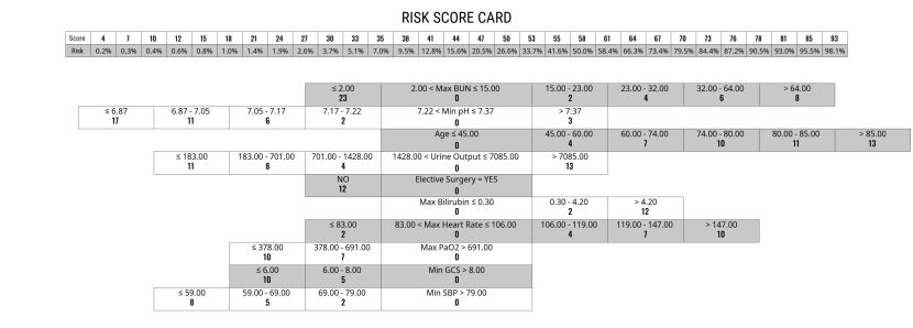
Figure 15: With group sparsity of 10. Both group sparsity and monotonicity constraints are applied.

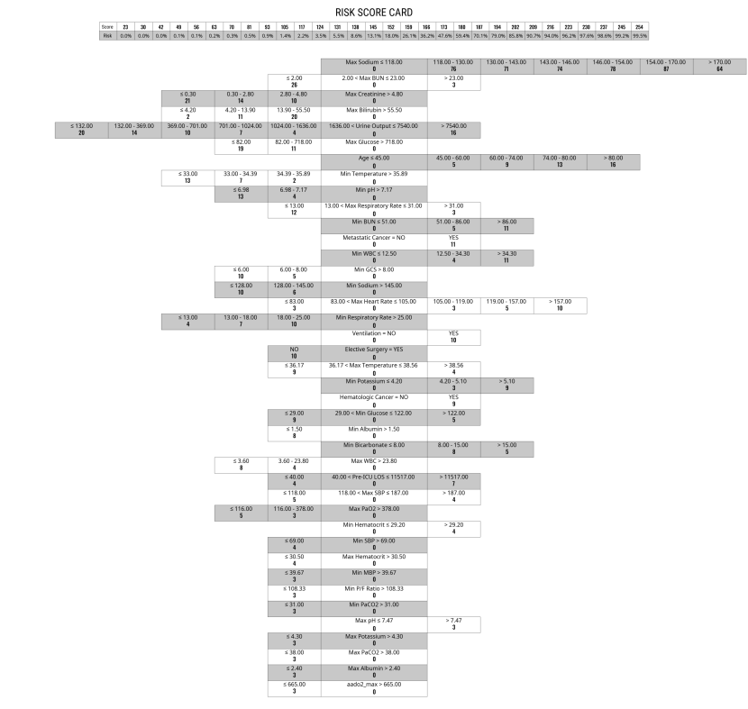
Figure 23: With group sparsity of 40. With group sparsity but without monotonicity constraints.

In this section, we perform an ablation study on the usefulness of our added functionality. Specifically, we run two sets of experiments: (1) vanilla FasterRisk [29] without group sparsity constraint nor monotonicity correction. (2) GroupFasterRisk with group sparsity constraint but without monotonicity correction. We present our results in terms of both tables (for quantitative measure of performances, see Table 5) and visualized risk scorecards (for qualitative measure of interpretability, see Figure 15 – Figure 23 in Section C.5).

Table 5: Ablation study on monotonicity correction. The evaluation is performed OOD on eICU. We observed a performance boost when monotonicity correction was applied, likely because correct domain information was included in the individual component scores of the features (see risk scorecard visualizations below).

Sparse Not Sparse GFR-10 OASIS GFR-15 SAPS II GFR-40 APACHE IV APACHE IVa $F=10$ $F=10$ $F=15$ $F=17$ $F=40$ $F=142$ $F=142$ With monotonicity correction AUROC 0.844 0.805 0.859 0.844 0.864 0.871 0.873 AUPRC 0.436 0.361 0.476 0.433 0.495 0.487 0.489 No monotonicity correction AUROC 0.840 0.805 0.857 0.844 0.863 0.871 0.873 AUPRC 0.427 0.361 0.467 0.433 0.491 0.487 0.489

C.2 Performance Comparisons

Table 6: GroupFasterRisk (not corrected with monotonicity constraints) compared with severity of illness scores under different group sparsity constraints. Evaluated on the internal MIMIC III dataset using 5-fold cross-validation, the best model from GroupFasterRisk is then evaluated OOD on the eICU dataset.
a. Hosmer-Lemeshow $\chi^{2}$ goodness of fit test, calculated using $C$ statistic (10 bins created from deciles of predicted probabilities) [38].
b. APACHE IV/IVa cannot be calculated on MIMIC III due to a lack of information for admission diagnoses.

Moderate Sparsity Not Sparse GFR-10 OASIS GFR-15 SAPS II GFR-40 APACHE IV APACHE IVa $F=10$ $F=10$ $F=15$ $F=17$ $F=40$ $F=142$ $F=142$ MIMIC III AUROC 0.813 $\pm$ 0.007 0.775 $\pm$ 0.008 0.836 $\pm$ 0.006 0.795 $\pm$ 0.009 0.858 $\pm$ 0.008 Test Folds AUPRC 0.368 $\pm$ 0.011 0.314 $\pm$ 0.014 0.403 $\pm$ 0.011 0.342 $\pm$ 0.012 0.443 $\pm$ 0.013 Brier Score 0.079 $\pm$ 0.001 0.086 $\pm$ 0.001 0.077 $\pm$ 0.001 0.102 $\pm$ 0.001 0.074 $\pm$ 0.001 HL^a $\chi^{2}$ 16.28 $\pm$ 2.51 146.16 $\pm$ 10.27 26.73 $\pm$ 6.38 691.45 $\pm$ 18.64 35.78 $\pm$ 11.01 SMR 0.992 $\pm$ 0.022 0.686 $\pm$ 0.008 0.996 $\pm$ 0.015 0.485 $\pm$ 0.005 1.002 $\pm$ 0.017 eICU AUROC 0.840 0.805 0.857 0.844 0.863 0.871 0.873 Test Set AUPRC 0.427 0.361 0.467 0.433 0.491 0.487 0.489

Table 7: Performance comparison with machine learning methods, evaluated using 5-fold nested cross-validation on MIMIC III dataset, the best model is evaluated out-of-sample on eICU dataset.
a. Hosmer-Lemeshow $\chi^{2}$ goodness of fit test, calculated using $C$ statistic [38].

GroupFasterRisk EBM XGBoost AdaBoost Random Forest LogReg ($\ell_{1}$) LogReg ($\ell_{2}$) MIMIC III AUROC 0.857 $\pm$ 0.008 0.871 $\pm$ 0.006 0.886 $\pm$ 0.005 0.870 $\pm$ 0.006 0.879 $\pm$ 0.004 0.863 $\pm$ 0.017 0.868 $\pm$ 0.006 Test Folds AUPRC 0.443 $\pm$ 0.013 0.476 $\pm$ 0.016 0.514 $\pm$ 0.022 0.472 $\pm$ 0.015 0.493 $\pm$ 0.012 0.458 $\pm$ 0.037 0.475 $\pm$ 0.020 Brier Score 0.074 $\pm$ 0.001 0.071 $\pm$ 0.001 0.073 $\pm$ 0.002 0.215 $\pm$ 0.0002 0.071 $\pm$ 0.001 0.072 $\pm$ 0.003 0.071 $\pm$ 0.002 HL^a $\chi^{2}$ 38.71 $\pm$ 13.88 27.69 $\pm$ 7.81 1569.00 $\pm$ 616.82 3488.69 $\pm$ 28.79 67.02 $\pm$ 10.43 30.01 $\pm$ 12.74 22.97 $\pm$ 4.42 SMR 1.006 $\pm$ 0.018 1.013 $\pm$ 0.013 1.858 $\pm$ 0.087 0.226 $\pm$ 0.0003 0.996 $\pm$ 0.008 1.000 $\pm$ 0.014 1.002 $\pm$ 0.019 eICU AUROC 0.863 0.878 0.885 0.878 0.883 0.870 0.871 Test Set AURPC 0.491 0.511 0.525 0.509 0.517 0.496 0.507 Brier Score 0.068 0.062 0.065 0.219 0.063 0.063 0.063 HL $\chi^{2}$ 3253.75 443.64 65437.29 68054.18 2220.83 315.65 885.87 SMR 0.664 0.856 1.786 0.199 0.780 0.876 0.798

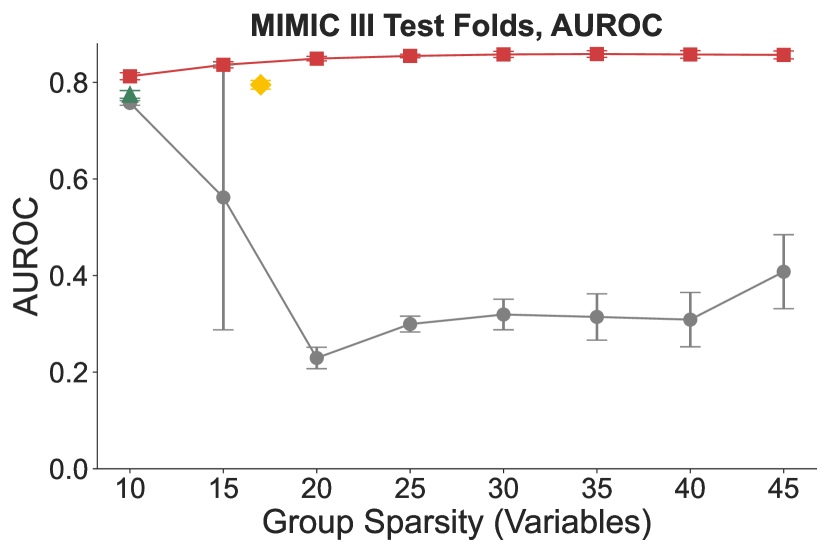
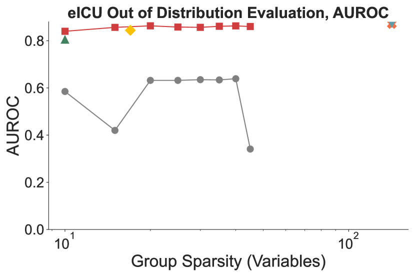
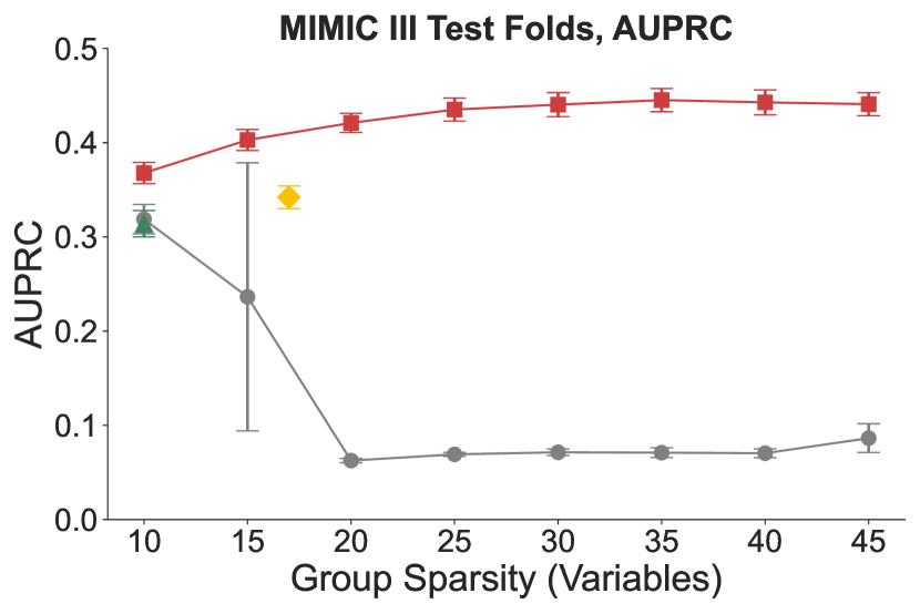
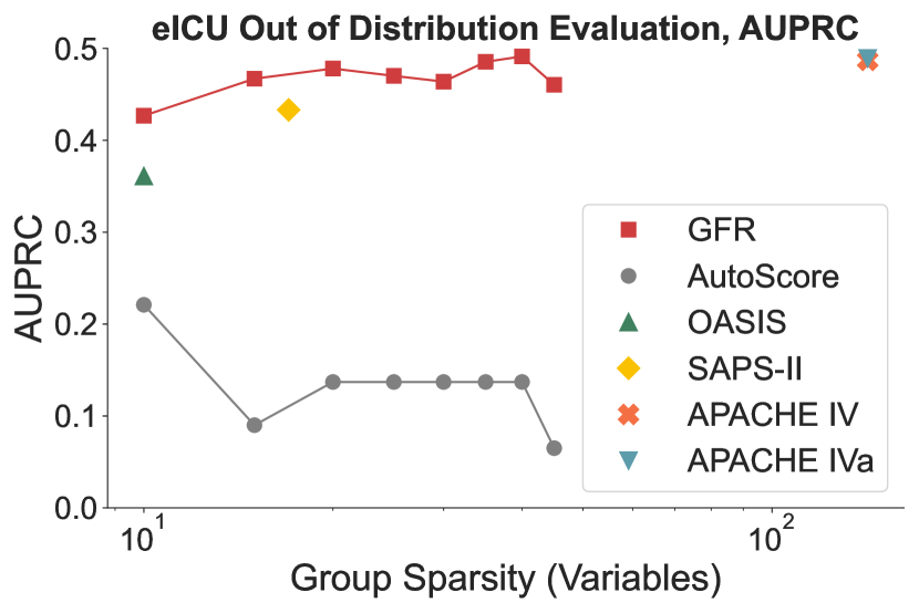
Figure 11: Performance of GroupFasterRisk under various values of group sparsity. We added a comparison with AutoScore [26] as an additional baseline. AutoScore is another automatic risk scorecard generation framework. At a high level, AutoScore creates risk scores by scaling logistic regression coefficients by the smallest of its real-valued coefficients, and it rounds coefficient values to the nearest integer afterward. A fine-tuning stage could be used by practitioners to adjust learned integer coefficients. We trained multiple AutoScore and GroupFasterRisk models at various group sparsity levels (number of features) and compared their performances. We found that GroupFasterRisk consistently outperformed AutoScore across all levels of group sparsity. AutoScore sometimes produces solutions where the AUROC is less than 0.5, which means that lower risk scores would actually imply higher risk outcomes, which is unintuitive. These observations show that without using the multiplier trick and smart rounding techniques, solutions tend to have poor qualities.

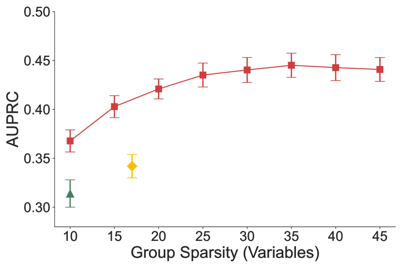
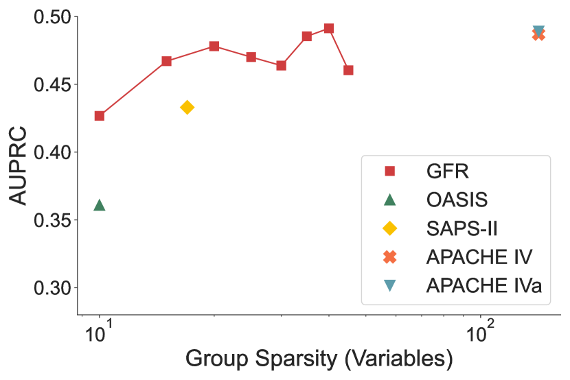
Figure 12: Performance under different group sparsities measured by AUPRC (without AutoScore). In this figure, we use AUPRC as the metric, which is different from Figure 6(a) that uses AUROC as the metric.

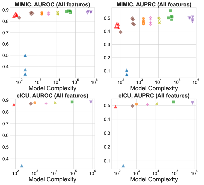
(a) Using all features.

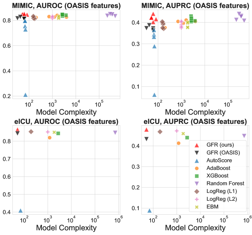
(b) Using OASIS features.

Figure 13: Complexity graph, GFR vs. ML algorithms. In this figure, GFR (ours) uses 19 variables, which is different from 14 variables used for Figure 9(a).

C.3 Fairness and Calibration Evaluations

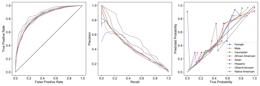
GFR-10 Fairness Performance.

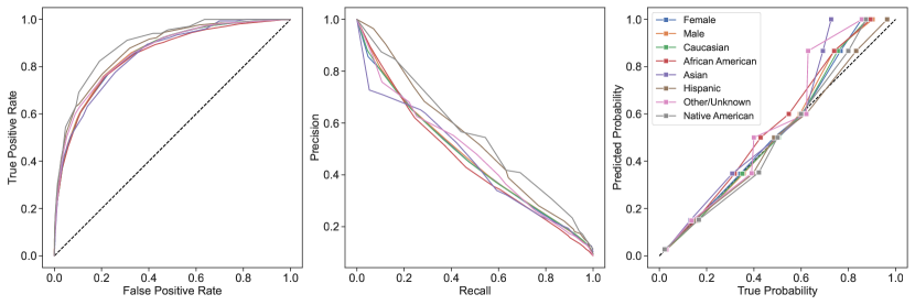
GFR-15 Fairness Performance.

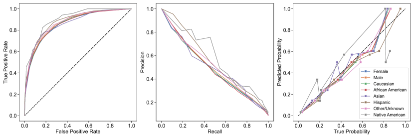
GFR-40 Fairness Performance.

Table 8: Out of distribution performance comparison with existing baselines. GroupFasterRisk is trained on disease-specific MIMIC subpopulation using various group sparsity constraints. We believe the drop in performance on the OOD on the eICU dataset is due to limited training data size on the MIMIC III sub-populations. Specifically, there are about 6,407 patients for acute kidney failure, 6,983 for heart failure, 3,505 for sepsis, and 3,625 for acute myocardial infarction, which is not enough to construct high-quality risk scores.

Low Sparsity Moderate Sparsity Not Sparse GFR-10 OASIS SOFA GFR-15 SAPS II GFR-40 APACHE IV APACHE IVa $F=10$ $F=10$ $F=11$ $F=15$ $F=17$ $F=40$ $F=142$ $F=142$ Sepsis/Septicemia AUROC 0.684 0.734 0.726 0.720 0.782 0.696 0.780 0.781 AUPRC 0.423 0.435 0.461 0.459 0.512 0.425 0.504 0.503 Acute Myocardial Infarction AUROC 0.858 0.846 0.795 0.814 0.879 0.785 0.879 0.886 AUPRC 0.409 0.424 0.395 0.375 0.493 0.342 0.493 0.498 Heart Failure AUROC 0.745 0.731 0.702 0.730 0.770 0.742 0.782 0.787 AUPRC 0.352 0.351 0.337 0.326 0.396 0.328 0.423 0.425 Acute Kidney Failure AUROC 0.739 0.760 0.723 0.763 0.781 0.765 0.803 0.802 AUPRC 0.485 0.472 0.462 0.479 0.527 0.511 0.552 0.550

Table 9: Fairness and calibration results across sub-groups in eICU study cohort. All models are calibrated using isotonic regression on 2,000 patients in the eICU cohort population, and evaluation is performed on the remaining population. Recall that in Table 2, we only calibrated GroupFasterRisk.

Ethnicity (alphabetical order) Gender African American Asian Caucasian Hispanic Native American Other/Unknown Female Male AUROC GFR-10 0.829 0.833 0.837 0.856 0.881 0.849 0.835 0.840 OASIS 0.811 0.797 0.803 0.825 0.824 0.809 0.806 0.805 GFR-15 0.846 0.848 0.854 0.873 0.895 0.860 0.853 0.856 SAPS II 0.846 0.828 0.843 0.859 0.893 0.842 0.844 0.845 GFR-40 0.859 0.861 0.859 0.881 0.902 0.873 0.857 0.865 APACHE IV 0.873 0.858 0.869 0.890 0.903 0.884 0.867 0.875 APACHE IVa 0.875 0.866 0.870 0.893 0.901 0.886 0.869 0.876 AUPRC GFR-10 0.415 0.390 0.422 0.480 0.558 0.418 0.418 0.429 OASIS 0.345 0.330 0.364 0.410 0.370 0.328 0.356 0.365 GFR-15 0.453 0.454 0.466 0.534 0.555 0.477 0.466 0.471 SAPS II 0.424 0.408 0.435 0.470 0.598 0.395 0.440 0.428 GFR-40 0.488 0.500 0.489 0.553 0.585 0.512 0.488 0.499 APACHE IV 0.488 0.467 0.484 0.536 0.536 0.479 0.478 0.493 APACHE IVa 0.487 0.492 0.487 0.538 0.522 0.484 0.481 0.496 Brier Score GFR-10 0.064 0.070 0.068 0.065 0.059 0.065 0.068 0.067 OASIS 0.068 0.076 0.072 0.069 0.071 0.070 0.072 0.070 GFR-15 0.062 0.068 0.065 0.061 0.059 0.061 0.065 0.064 SAPS II 0.064 0.071 0.068 0.065 0.057 0.067 0.067 0.067 GFR-40 0.060 0.064 0.064 0.060 0.057 0.059 0.064 0.062 APACHE IV 0.060 0.067 0.064 0.059 0.061 0.061 0.064 0.062 APACHE IVa 0.060 0.065 0.064 0.060 0.060 0.061 0.064 0.062 HL $\chi^{2}$ GFR-10 27.90 11.00 113.70 24.68 5.48 12.53 58.65 102.74 OASIS 12.89 19.16 41.68 13.47 4.39 8.19 26.37 25.26 GFR-15 23.64 9.88 63.40 10.62 4.43 3.73 13.62 57.75 SAPS II 70.37 19.94 193.09 21.58 6.28 44.37 118.68 130.72 GFR-40 8.72 5.20 120.03 12.03 11.57 6.09 58.34 97.92 APACHE IV 82.93 15.15 273.84 15.17 21.69 40.82 169.04 253.34 APACHE IVa 47.89 7.75 100.27 6.25 14.24 19.45 78.47 46.56 SMR GFR-10 0.946 0.915 1.028 1.017 0.949 1.013 0.993 1.031 OASIS 0.952 1.276 1.000 1.069 0.928 1.075 0.995 1.014 GFR-15 0.974 0.921 1.040 1.046 1.003 0.996 1.002 1.046 SAPS II 0.941 1.096 0.986 1.082 0.950 1.056 1.004 0.981 GFR-40 1.022 0.936 1.039 1.063 0.889 1.033 1.000 1.058 APACHE IV 0.891 0.997 1.003 0.962 0.792 0.952 0.983 0.988 APACHE IVa 0.876 1.001 1.006 0.947 0.849 0.938 0.979 0.991

C.4 GroupFasterRisk Performances

Table 10: GroupFasterRisk performance under various bin widths. To allow GroupFasterRisk to better utilize continuous variables, a binarization technique is applied, which transforms a continuous variable into $B$ quantiles (bins). The experiment is conducted using 5 fold cross validation on MIMIC III training and validation folds; each cross validation gives a mean AUROC and AUPRC. Each $B$ represents a fixed combination of group sparsity and sparsity constraints, and the mean and standard deviation of all those runs is reported.

Number of Bins ($B$) 100 50 20 10 5 4 Average Mean AUROC Training 0.847 $\pm$ 0.030 0.849 $\pm$ 0.029 0.856 $\pm$ 0.020 0.850 $\pm$ 0.023 0.847 $\pm$ 0.016 0.841 $\pm$ 0.019 Validation 0.828 $\pm$ 0.030 0.832 $\pm$ 0.028 0.843 $\pm$ 0.018 0.839 $\pm$ 0.022 0.840 $\pm$ 0.015 0.835 $\pm$ 0.018 Average Mean AUPRC Training 0.444 $\pm$ 0.057 0.448 $\pm$ 0.056 0.451 $\pm$ 0.043 0.439 $\pm$ 0.046 0.430 $\pm$ 0.032 0.413 $\pm$ 0.036 Validation 0.394 $\pm$ 0.047 0.401 $\pm$ 0.047 0.414 $\pm$ 0.033 0.413 $\pm$ 0.037 0.412 $\pm$ 0.028 0.401 $\pm$ 0.032

C.5 Visualizations of Risk Scores Generated by GroupFasterRisk

In this section, we present the risk scores generated by GroupFasterRisk for group sparsity of 10, 15, 40 (Section C.5.1) as well as visualize the score cards a part of our ablation study discussed in Section C.1. Specifically, we present three sets of risk scores to highlight the usefulness of group sparsity and monotonicity constraints:

1. Risk scores generated with both group sparsity and monotonicity constraints, Section C.5.1. These models correspond to those produced by GroupFasterRisk.

2. Risk scores generated with neither group sparsity nor monotonicity constraints, Section C.5.2. Here, we do not optimize for group sparsity constraints $\gamma$ that we discussed in Section 4.1 and do not apply monotonic correction (Section 4.4).

3. Risk scores generated with only group sparsity and without monotonicity constraints, Section C.5.3. Here, we do not apply monotonic correction that we discussed in Section 4.4.

For each set, we use group sparsity of 10, 15, and 40. In Section C.5.1, for risk scores with group sparsity of 10, we apply monotonicity constraints on Max Bilirubin, Min GCS, and Min SBP. For a group sparsity of 15, we apply monotonicity constraints on Max Bilirubin, Min GCS, Min SBP, and Max BUN. For a group sparsity of 40, we apply monotonicity constraints on Max Bilirubin, Max Sodium, Min Respiratory Rate, and Min Bicarbonate.

We observe that the addition of group sparsity constraints allows us to create more cohesive risk scores, and monotonicity constraints allow for the inclusion of medical domain knowledge into the risk score. For instance, when not using monotonicity constraints, we observe that the model creates risk scores that predict a lower risk for patients with minimum Glascow Coma Score (GCS) of 3 than those with higher minimum GCS. This is partly due to the training dataset, which has fewer samples with minimum GCS of 3 than those with minimum GCS between 3 and 6. Thus, this relationship is often reflected by models trained without monotonicity constraints. Luckily, due to the interpretable nature of our model, we can notice this easily and apply monotonicity constraints to correct it.

C.5.1 With both group sparsity and monotonicity constraints

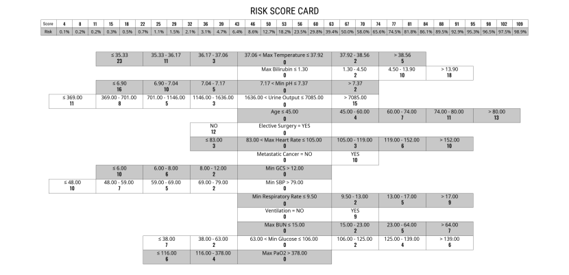
Figure 16: With group sparsity of 15. Both group sparsity and monotonicity constraints are applied.

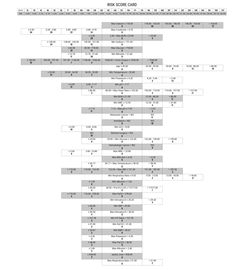
Figure 17: With group sparsity of 40. Both group sparsity and monotonicity constraints are applied.

C.5.2 With neither group sparsity nor monotonicity constraints

We trained GroupFasterRisk models without group sparsity and monotonicity constraints to indicate the usefulness of these functionalities in risk score generation. For direct and fair comparisons, we set all of the hyperparameters (other than $\gamma$ and $({\bm{a}},{\bm{b}})$) the same as those used in Section C.5.1.

Observe that the risk scores are less cohesive (more features, fewer options per feature) than the ones trained with group sparsity constraints. In particular, the user loses control over the total number of component functions for the risk score. Additionally, without monotonicity, the component functions may reflect noise in the data that does not align with domain knowledge. For instance, Figure 20 has a risk score that decreases even when Min Respiratory Rate is dangerously low.

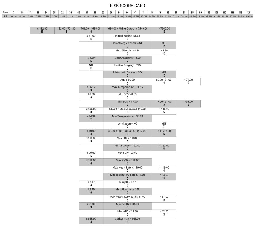
Figure 18: With the same hyperparameters as the previous model with group sparsity of 10 in Section C.5.1. Neither group sparsity nor monotonicity constraints are applied.

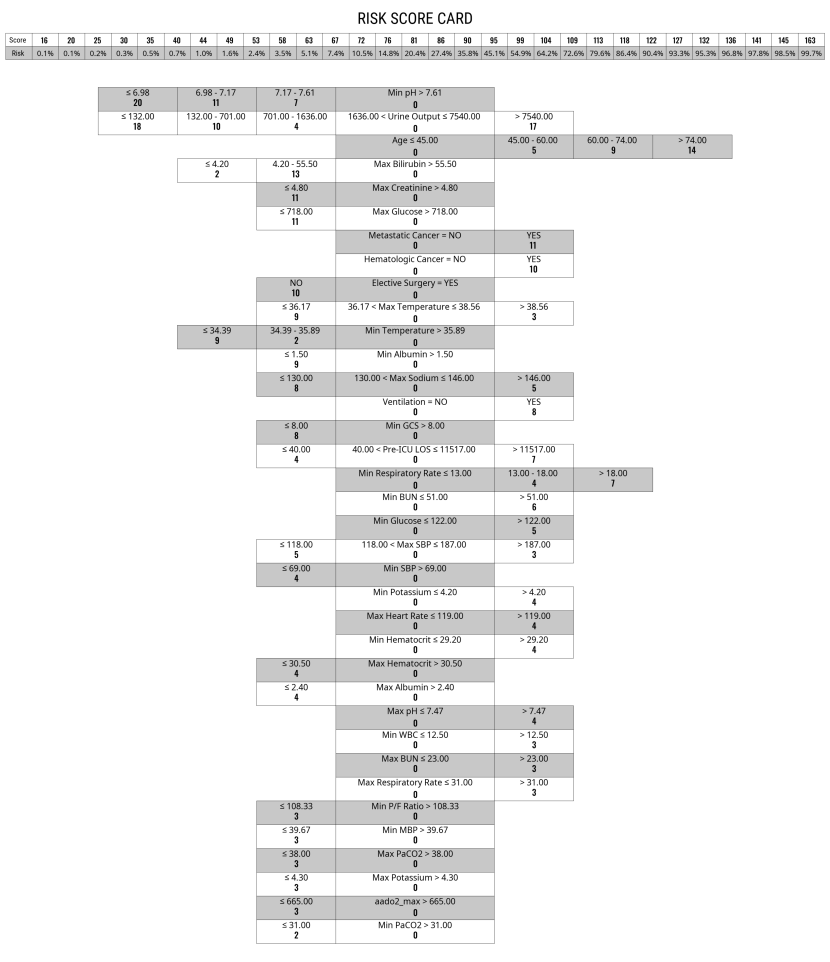
Figure 19: With the same hyperparameters as the previous model with group sparsity of 15 in Section C.5.1. Neither group sparsity nor monotonicity constraints are applied.

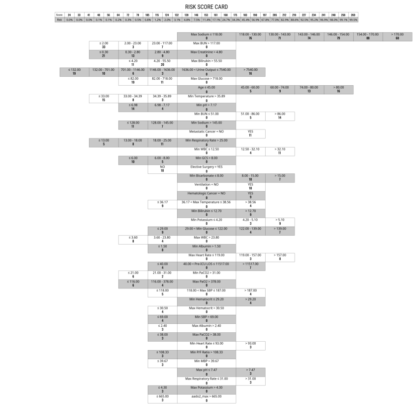
Figure 20: With the same hyperparameters as the previous model with group sparsity of 40 in Section C.5.1. Neither group sparsity nor monotonicity constraints are applied.

C.5.3 With only group sparsity and without monotonicity constraints

We trained GroupFasterRisk models with group sparsity but without monotonicity constraints. This enables us to see the usefulness of monotonicity correction. For direct and fair comparisons, we set all of the hyperparameters (other than $({\bm{a}},{\bm{b}})$) the same as those used in Section C.5.1.

Observe that the model in Figure 21 predicts lower risk for patients with minimum GCS of 3 than those with minimum GCS between 3 and 6.

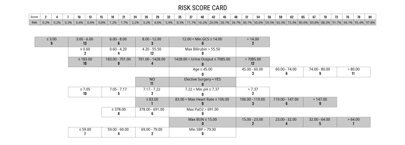
Figure 21: With group sparsity of 10. With group sparsity but without monotonicity constraints.

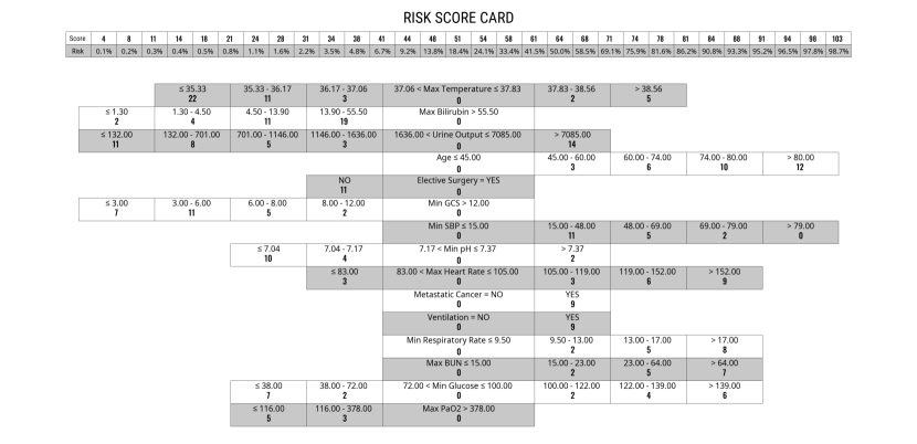
Figure 22: With group sparsity of 15. With group sparsity but without monotonicity constraints.

References

- [1] Robert L McNamara et al. “Predicting in-hospital mortality in patients with acute myocardial infarction” In Journal of the American College of Cardiology 68.6 American College of Cardiology Foundation Washington, DC, 2016, pp. 626–635
- [2] Fred H Edwards et al. “Development and validation of a risk prediction model for in-hospital mortality after transcatheter aortic valve replacement” In JAMA Cardiology 1.1 American Medical Association, 2016, pp. 46–52
- [3] Gregg C Fonarow et al. “Risk stratification for in-hospital mortality in acutely decompensated heart failure: classification and regression tree analysis” In JAMA 293.5 American Medical Association, 2005, pp. 572–580
- [4] Steven L Barriere and Stephen F Lowry “An overview of mortality risk prediction in sepsis” In Critical Care Medicine 23.2 LWW, 1995, pp. 376–393
- [5] Ali A El-Solh et al. “Comparison of in-hospital mortality risk prediction models from COVID-19” In PloS One 15.12 Public Library of Science San Francisco, CA USA, 2020, pp. e0244629
- [6] Sujoy Kar et al. “Multivariable mortality risk prediction using machine learning for COVID-19 patients at admission (AICOVID)” In Scientific Reports 11.1 Nature Publishing Group UK London, 2021, pp. 12801
- [7] William A Knaus et al. “APACHE—acute physiology and chronic health evaluation: a physiologically based classification system” In Critical Care Medicine 9.8 LWW, 1981, pp. 591–597
- [8] J -L Vincent et al. “The SOFA (Sepsis-related Organ Failure Assessment) score to describe organ dysfunction/failure: On behalf of the Working Group on Sepsis-Related Problems of the European Society of Intensive Care Medicine (see contributors to the project in the appendix)” Springer-Verlag, 1996
- [9] Mervyn Singer et al. “The third international consensus definitions for sepsis and septic shock (Sepsis-3)” In JAMA 315.8 American Medical Association, 2016, pp. 801–810
- [10] William A Knaus, Elizabeth A Draper, Douglas P Wagner and Jack E Zimmerman “APACHE II: a severity of disease classification system.” In Critical Care Medicine 13.10, 1985, pp. 818–829
- [11] Jean-Roger Le Gall et al. “A simplified acute physiology score for ICU patients.” In Critical Care Medicine 12.11, 1984, pp. 975–977
- [12] Jack E Zimmerman, Andrew A Kramer, Douglas S McNair and Fern M Malila “Acute Physiology and Chronic Health Evaluation (APACHE) IV: hospital mortality assessment for today’s critically ill patients” In Critical Care Medicine 34.5 LWW, 2006, pp. 1297–1310
- [13] William S Cleveland “Robust locally weighted regression and smoothing scatterplots” In Journal of the American Statistical Association 74.368 Taylor & Francis, 1979, pp. 829–836
- [14] Alistair EW Johnson, Andrew A Kramer and Gari D Clifford “A new severity of illness scale using a subset of acute physiology and chronic health evaluation data elements shows comparable predictive accuracy” In Critical Care Medicine 41.7 LWW, 2013, pp. 1711–1718
- [15] Sourabh Katoch, Sumit Singh Chauhan and Vijay Kumar “A review on genetic algorithm: past, present, and future” In Multimedia Tools and Applications 80 Springer, 2021, pp. 8091–8126
- [16] James Kennedy and Russell Eberhart “Particle swarm optimization” In Proceedings of ICNN’95-International Conference on Neural Networks 4, 1995, pp. 1942–1948 IEEE
- [17] Min Hyuk Choi et al. “Mortality prediction of patients in intensive care units using machine learning algorithms based on electronic health records” In Scientific Reports 12.1 Nature Publishing Group UK London, 2022, pp. 7180
- [18] Yasser El-Manzalawy et al. “OASIS+: leveraging machine learning to improve the prognostic accuracy of OASIS severity score for predicting in-hospital mortality” In BMC Medical Informatics and Decision Making 21.1 Springer, 2021, pp. 156
- [19] Scott Levin et al. “Machine-learning-based electronic triage more accurately differentiates patients with respect to clinical outcomes compared with the emergency severity index” In Annals of Emergency Medicine 71.5 Elsevier, 2018, pp. 565–574
- [20] Maximiliano Klug et al. “A gradient boosting machine learning model for predicting early mortality in the emergency department triage: devising a nine-point triage score” In Journal of General Internal Medicine 35 Springer, 2020, pp. 220–227
- [21] Woo Suk Hong, Adrian Daniel Haimovich and R Andrew Taylor “Predicting hospital admission at emergency department triage using machine learning” In PloS One 13.7 Public Library of Science San Francisco, CA USA, 2018, pp. e0201016
- [22] José A González-Nóvoa et al. “Using explainable machine learning to improve intensive care unit alarm systems” In Sensors 21.21 Multidisciplinary Digital Publishing Institute, 2021, pp. 7125
- [23] Leo Breiman “Random forests” In Machine Learning 45 Springer, 2001, pp. 5–32
- [24] Tianqi Chen et al. “Xgboost: extreme gradient boosting” In R package version 0.4-2 1.4, 2015, pp. 1–4
- [25] Cynthia Rudin “Stop explaining black box machine learning models for high stakes decisions and use interpretable models instead” In Nature Machine Intelligence 1.5 Nature Publishing Group UK London, 2019, pp. 206–215
- [26] Feng Xie et al. “AutoScore: a machine learning–based automatic clinical score generator and its application to mortality prediction using electronic health records” In JMIR Medical Informatics 8.10 JMIR Publications Inc., Toronto, Canada, 2020, pp. e21798
- [27] Berk Ustun and Cynthia Rudin “Optimized risk scores” In Proceedings of the 23rd ACM SIGKDD international conference on knowledge discovery and data mining, 2017, pp. 1125–1134
- [28] Berk Ustun and Cynthia Rudin “Learning Optimized Risk Scores.” In J. Mach. Learn. Res. 20.150, 2019, pp. 1–75
- [29] Jiachang Liu et al. “FasterRisk: Fast and Accurate Interpretable Risk Scores” In Advances in Neural Information Processing Systems 35 Curran Associates, Inc., 2022, pp. 17760–17773
- [30] Alistair EW Johnson et al. “MIMIC-III, a freely accessible critical care database” In Scientific Data 3.1 Nature Publishing Group, 2016, pp. 1–9
- [31] Tom J Pollard et al. “The eICU Collaborative Research Database, a freely available multi-center database for critical care research” In Scientific Data 5.1 Nature Publishing Group, 2018, pp. 1–13
- [32] Jesse Davis and Mark Goadrich “The relationship between Precision-Recall and ROC curves” In Proceedings of the 23rd International Conference on Machine Learning, 2006, pp. 233–240
- [33] Yin Lou, Rich Caruana and Johannes Gehrke “Intelligible models for classification and regression” In Proceedings of the 18th ACM SIGKDD International Conference on Knowledge Discovery and Data Mining, 2012, pp. 150–158
- [34] Tianqi Chen and Carlos Guestrin “Xgboost: A scalable tree boosting system” In Proceedings of the 22nd ACM SIGKDD International Conference on Knowledge Discovery and Data Mining, 2016, pp. 785–794
- [35] Yoav Freund and Robert E Schapire “A decision-theoretic generalization of on-line learning and an application to boosting” In Journal of Computer and System Sciences 55.1 Elsevier, 1997, pp. 119–139
- [36] Yingxiang Huang et al. “A tutorial on calibration measurements and calibration models for clinical prediction models” In Journal of the American Medical Informatics Association 27.4 Oxford University Press, 2020, pp. 621–633
- [37] Glenn W Brier “Verification of forecasts expressed in terms of probability” In Monthly Weather Review 78.1, 1950, pp. 1–3
- [38] Stanley Lemeshow and David W Hosmer Jr “A review of goodness of fit statistics for use in the development of logistic regression models” In American Journal of Epidemiology 115.1 Oxford University Press, 1982, pp. 92–106
- [39] Cynthia Rudin et al. “Interpretable machine learning: Fundamental principles and 10 grand challenges” In Statistic Surveys 16 The American Statistical Association, the Bernoulli Society, the Institute …, 2022, pp. 1–85
- [40] Aaron Fisher, Cynthia Rudin and Francesca Dominici “All Models are Wrong, but Many are Useful: Learning a Variable’s Importance by Studying an Entire Class of Prediction Models Simultaneously.” In Journal of Machine Learning Research 20.177, 2019, pp. 1–81
- [41] Lesia Semenova, Cynthia Rudin and Ronald Parr “On the existence of simpler machine learning models” In Proceedings of the 2022 ACM Conference on Fairness, Accountability, and Transparency, 2022, pp. 1827–1858
- [42] Jean-Roger Le Gall, Stanley Lemeshow and Fabienne Saulnier “A new simplified acute physiology score (SAPS II) based on a European/North American multicenter study” In JAMA 270.24 American Medical Association, 1993, pp. 2957–2963
- [43] Christopher W Seymour et al. “Assessment of clinical criteria for sepsis: for the Third International Consensus Definitions for Sepsis and Septic Shock (Sepsis-3)” In JAMA 315.8 American Medical Association, 2016, pp. 762–774
- [44] Yin Lou, Rich Caruana, Johannes Gehrke and Giles Hooker “Accurate intelligible models with pairwise interactions” In Proceedings of the 19th ACM SIGKDD International Conference on Knowledge Discovery and Data Mining, 2013, pp. 623–631
- [45] Yee-Chun Chen et al. “Risk factors for ICU mortality in critically ill patients” In Journal of the Formosan Medical Association 100.10 FORMOSAN MEDICAL ASSOCIATION, 2001, pp. 656–661
- [46] Derek C Angus et al. “Epidemiology of severe sepsis in the United States: analysis of incidence, outcome, and associated costs of care” In Critical Care Medicine 29.7 LWW, 2001, pp. 1303–1310
- [47] Writing Group Members et al. “Heart disease and stroke statistics—2012 update: a report from the American Heart Association” In Circulation 125.1 Am Heart Assoc, 2012, pp. e2–e220
- [48] John C Marshall et al. “Multiple organ dysfunction score: a reliable descriptor of a complex clinical outcome” In Critical Care Medicine 23.10 LWW, 1995, pp. 1638–1652
- [49] Rinaldo Bellomo et al. “Acute renal failure–definition, outcome measures, animal models, fluid therapy and information technology needs: the Second International Consensus Conference of the Acute Dialysis Quality Initiative (ADQI) Group” In Critical Care 8.4 BioMed Central, 2004, pp. 1–9
- [50] Lilian Minne, Ameen Abu-Hanna and Evert Jonge “Evaluation of SOFA-based models for predicting mortality in the ICU: A systematic review” In Critical Care 12.6 BioMed Central, 2008, pp. 1–13
- [51] Mohamed Fayed et al. “Sequential organ failure assessment (SOFA) score and mortality prediction in patients with severe respiratory distress secondary to COVID-19” In Cureus 14.7 Cureus, 2022
- [52] Ninareh Mehrabi et al. “A survey on bias and fairness in machine learning” In ACM Computing Surveys (CSUR) 54.6 ACM New York, NY, USA, 2021, pp. 1–35
- [53] Yizhao Zhou et al. “Missing data matter: an empirical evaluation of the impacts of missing EHR data in comparative effectiveness research” In Journal of the American Medical Informatics Association Oxford University Press, 2023, pp. ocad066
- [54] Stef Van Buuren and Karin Groothuis-Oudshoorn “mice: Multivariate imputation by chained equations in R” In Journal of Statistical Software 45, 2011, pp. 1–67
- [55] Wei-Chao Lin and Chih-Fong Tsai “Missing value imputation: a review and analysis of the literature (2006–2017)” In Artificial Intelligence Review 53 Springer, 2020, pp. 1487–1509
- [56] George A Miller “The magical number seven, plus or minus two: Some limits on our capacity for processing information.” In Psychological Review 63.2 American Psychological Association, 1956, pp. 81
- [57] Nelson Cowan “The magical mystery four: How is working memory capacity limited, and why?” In Current Directions in Psychological Science 19.1 Sage Publications Sage CA: Los Angeles, CA, 2010, pp. 51–57
- [58] Zijie J Wang et al. “Interpretability, then what? editing machine learning models to reflect human knowledge and values” In Proceedings of the 28th ACM SIGKDD Conference on Knowledge Discovery and Data Mining, 2022, pp. 4132–4142
- [59] Joseph Futoma et al. “The myth of generalisability in clinical research and machine learning in health care” In The Lancet Digital Health 2.9 Elsevier, 2020, pp. e489–e492
- [60] Bret Nestor et al. “Feature robustness in non-stationary health records: caveats to deployable model performance in common clinical machine learning tasks” In Machine Learning for Healthcare Conference, 2019, pp. 381–405 PMLR
- [61] William A Knaus et al. “The APACHE III prognostic system: risk prediction of hospital mortality for critically III hospitalized adults” In Chest 100.6 Elsevier, 1991, pp. 1619–1636
- [62] Jean-Roger Le Gall et al. “The Logistic Organ Dysfunction system: a new way to assess organ dysfunction in the intensive care unit” In JAMA 276.10 American Medical Association, 1996, pp. 802–810
- [63] Roger C Bone et al. “Definitions for sepsis and organ failure and guidelines for the use of innovative therapies in sepsis” In Chest 101.6 Elsevier, 1992, pp. 1644–1655
- [64] Trevor J Hastie and Robert J Tibshirani “Generalized additive models” CRC press, 1990
- [65] Caroline Wang, Bin Han, Bhrij Patel and Cynthia Rudin “In pursuit of interpretable, fair and accurate machine learning for criminal recidivism prediction” In Journal of Quantitative Criminology Springer, 2022, pp. 1–63