Sum-of-Squares Lower Bounds for
the Minimum Circuit Size Problem

Abstract

We prove lower bounds for the Minimum Circuit Size Problem (MCSP) in the Sum-of-Squares (SoS) proof system. Our main result is that for every Boolean function $f:\{0,1\}^{n}\rightarrow\{0,1\}$, SoS requires degree $\Omega(s^{1-\epsilon})$ to prove that $f$ does not have circuits of size $s$ (for any $s>\poly(n)$). As a corollary we obtain that there are no low degree SoS proofs of the statement $\NP\not\subseteq\Ppoly$.

We also show that for any $0<\alpha<1$ there are Boolean functions with circuit complexity larger than $2^{n^{\alpha}}$ but SoS requires size $2^{2^{\Omega(n^{\alpha})}}$ to prove this. In addition we prove analogous results on the minimum monotone circuit size for monotone Boolean slice functions.

Our approach is quite general. Namely, we show that if a proof system $Q$ has strong enough constraint satisfaction problem lower bounds that only depend on good expansion of the constraint-variable incidence graph and, furthermore, $Q$ is expressive enough that variables can be substituted by local Boolean functions, then the MCSP problem is hard for $Q$.

1 Introduction

Even before the dawn of complexity theory, there was an interest in the minimum circuit size problem (MCSP): given the truth table of a Boolean function $f:\{0,1\}^{n}\rightarrow\{0,1\}$ and a parameter $s$, the MCSP problem asks whether there is a Boolean circuit of size at most $s$ computing $f$. Despite many years of research, we do not know whether this problem is -hard. It clearly is in : given a circuit of size at most $s$ (described by $O(s\log s)$ bits) we can easily check in time $O(s\cdot 2^{n})$ whether this circuit indeed computes $f$.

Determining the hardness of MCSP itself turns out to be a difficult problem. Kabanets and Cai [KC00] showed that -hardness of the MCSP problem implies breakthrough circuit lower bounds. These lower bounds are not implausible but well out of reach of current techniques. In a similar vein Murray and Williams [MW15] showed that -hardness of MCSP implies that $\EXP\neq\ZPP$ and more recently Hirahara [Hir18] proved that -hardness of MCSP implies a worst-case to average-case reduction for problems in  (for an appropriate MCSP version).

On the other hand if one could show that MCSP is in , this would imply even stronger (though less realistic) results: Kabanets and Cai [KC00] also showed that if MCSP is in , then crypto-secure one way functions can be inverted on a considerable fraction of their range.

To summarize it seems unlikely that MCSP is in ¶, but showing that it is -hard implies very strong consequences. As these results seem out of reach for current techniques, it might be a more fruitful avenue to try to at least rule out that certain (families of) algorithms solve the MCSP problem efficiently.

This can be achieved very elegantly in proof complexity: show that some proof system capturing your algorithm requires long proofs to refute the claim that a complex function has a small circuit. This will then rule out that the algorithm in question can efficiently solve the MCSP problem. This will not only show that this specific algorithm requires long running time but would also show that any algorithm captured by this proof system requires long running time to solve the MCSP problem. Hence by this line of reasoning we manage to rule out entire classes of algorithms to solve the MCSP problem efficiently.

This paper focuses on the Sum of Squares proof system (SoS). This proof system provides certificates of unsatisfiability of systems of polynomial equations $\mathcal{P}=\{p_{1}=0,\ldots,p_{m}=0\}$ over $\mathbb{R}$. In this paper we are only interested in Boolean systems of equations, meaning that $\mathcal{P}$ contains the equation $x^{2}-x=0$ for every variable $x$ appearing in the system. A key complexity measure is the degree of a refutation, which is the maximum degree of a monomial occurring in the refutation of $\mathcal{P}$. All Boolean systems $\mathcal{P}$ over $n$ variables have an SoS refutation of degree $n$ and we are interested in the minimum degree that SoS requires to refute $\mathcal{P}$. An SoS refutation of degree $d$ has size $O(n^{d})$ and can be found in $n^{O(d)}$ time using semidefinite programming and this is often a useful heuristic bound for the complexity of an SoS refutation. The actual size complexity of SoS can sometimes be significantly smaller than $n^{d}$ [Pot20] and it would be surprising if the shortest refutation can be found efficiently. Hence it is in general of interest to understand both the degree and the size needed to refute any given system.

SoS is a very powerful proof system and captures many state of the art algorithms that are based on spectral methods. A classic algorithm captured by SoS is Goemans and Williamson’s Max-Cut algorithm [GW95], but also approximate graph coloring algorithms [KMS98], and algorithms solving constraint satisfaction problems [AOW15, RRS17] are captured by SoS. On the other hand SoS has real difficulty arguing about integers and in particular parities. Indeed, Grigoriev [Gri01] showed that SoS requires degree $\Omega(n)$ to refute a random xor constraint satisfaction problem of the appropriate (constant) density. After this initial lower bound it took a few years to develop good lower bounds methods for SoS, but in recent years there has been a flurry of strong SoS degree lower bounds [MPW15, BHK⁺16, KMOW17].

In order to rule out that algorithms captured by SoS can solve MCSP efficiently, we need to encode the claim that a given function has a small circuit as a propositional formula. We work with the encoding suggested by Razborov [Raz98], which encodes this claim that the function $f:\{0,1\}^{n}\rightarrow\{0,1\}$ has a circuit of size $s$ by a propositional formula $\operatorname{Circuit}_{s}(f)$ over $O(s^{2}+s\cdot 2^{n})=O(s\cdot 2^{n})$ variables as follows. We have $\Theta(s^{2})$ structure variables to encode all possible size $s$ circuits, and for every assignment $\alpha\in\{0,1\}^{n}$ we then have an additional $\Theta(s)$ evaluation variables that simulate the evaluation of the circuit on each input, and constraints forcing the circuit to output the correct value on each input $\alpha$.

A closely related question to the MCSP problem is the question of how hard it is to actually prove strong circuit lower bounds. For example, are there efficient refutations of the statement $\NP\subseteq\Ppoly$, assuming the statement is false? This question, as proposed by Razborov [Raz98], can also be investigated by studying above formula: consider $\operatorname{Circuit}_{n^{O(1)}}(\SAT)$, where $\SAT$ is the function that outputs $1$ if and only if the input is an encoding of a satisfiable CNF. This is, essentially, a propositional encoding of the claim that $\SAT$ has a circuit in $\Ppoly$. Hence proving lower bounds for $\operatorname{Circuit}_{n^{O(1)}}(\SAT)$ rules out efficient proofs of $\NP\not\subseteq\Ppoly$ in the proof system under consideration.

Experience suggests that studying such meta-mathematical questions is difficult. This problem is no exception to this rule and, even though the formula has been conjectured to be hard for strong proof systems such as extended Frege, progress has been slow. The only proof systems for which we have unconditional, superpolynomial lower bounds on proofs of the $\operatorname{Circuit}_{s}(f)$ formula are Resolution [Raz04a, Raz04b], small width DNF-Resolution [Raz15] and Polynomial Calculus [Raz98, Raz15]. The resolution size and Polynomial Calculus degree lower bounds follow from a reduction of the pigeonhole principle to $\operatorname{Circuit}_{s}(f)$. In fact, this reduction was a main motivation for a long line of work [RWY02, PR04, Raz04a, Raz04b] eventually establishing strong resolution lower bounds for the weak pigeonhole principle. The other size lower bounds follow from a general connection between pseudo-random generator lower bounds and MCSP lower bounds as outlined in [ABRW04, Raz15], building on Krajíček’s iterability trick [Kra01].

As the pigeonhole principle is easy for the SoS proof system [GHP02], we cannot hope to borrow the hardness from that formula. Neither do we have strong enough pseudorandom generator lower bounds for SoS to employ that connection. In fact, to date, we have no unconditional (degree) lower bounds for any semi-algebraic proof system, that is, proof systems that manipulate polynomial inequalities such as SoS or Cutting Planes. Furthermore it has been stated [Raz21, Raz22] as an explicit open problem to prove SoS degree lower bounds for the formula $\operatorname{Circuit}_{s}(f)$.

1.1 Our Results

Our first result gives a lower bound on the degree needed to refute $\operatorname{Circuit}_{s}(f)$ in SoS. This lower bound is very general and in fact applies to every Boolean function $f:\{0,1\}^{n}\rightarrow\{0,1\}$.

Theorem 1.1.

For all $\varepsilon>0$ there is a $d=d(\varepsilon)$ such that the following holds. For $n\in\mathbb{N}$, all $s\geq n^{d}$ and any Boolean function $f:\{0,1\}^{n}\rightarrow\{0,1\}$ on $n$ bits, SoS requires degree $\Omega_{\varepsilon}(s^{1-\varepsilon})$ to refute $\operatorname{Circuit}_{s}(f)$.

It is worthwhile to point out that the proof of Theorem 1.1 is not specific to the SoS proof system. In fact we outline a general reduction that shows that if one has a CSP lower bound of the form of Theorem 2.8 that only requires good expansion of the underlying constraint-variable incidence graph and the proof system is expressive enough so that one can replace variables by local Boolean functions, then one obtains strong lower bounds for the $\operatorname{Circuit}_{s}(f)$ formula.

The lower bound of $\Omega_{\varepsilon}(s^{1-\varepsilon})$ on the degree is essentially tight: if $f$ does not have a circuit of size $s$ then there exists an SoS refutation of this statement in degree $O(s)$.

Proposition 1.2.

Let $s\in N$ and $f:\{0,1\}^{n}\rightarrow\{0,1\}$ be a Boolean function on $n$ bits that requires circuits of size larger than $s$ to be computed. Then there is a degree $O(s)$ SoS refutation of $\operatorname{Circuit}_{s}(f)$.

We also prove a result about the minimum size (number of monomials) required for SoS to refute $\operatorname{Circuit}_{s}(f)$. This result holds for all functions that “almost” have a circuit of size $s$, in the sense that they have an errorless heuristic circuit (see the survey [BT06]) of size $s/2$ and extremely small error probability with respect to the uniform distribution. Formally, we let $\mathcal{F}_{n}(s,t)$ denote the class of Boolean functions that consists of all functions $f:\{0,1\}^{n}\rightarrow\{0,1\}$ for which there is a Boolean circuit $C_{f}:\{0,1\}^{n}\rightarrow\{0,1,\bot\}$ of size at most $s$ such that

1. if $C_{f}(\alpha)\neq\bot$, then $C_{f}(\alpha)=f(\alpha)$, and

2. $C_{f}(\alpha)=\bot$ on at most $t$ inputs.

In other words the circuit $C_{f}$ computes $f$ correctly on all except $t$ inputs. Note that technically the output of the circuit $C_{f}$ is two bits with the first one indicating whether the output is $\bot$ or the value of the second bit. We believe that above presentation is more intuitive and hope that the slight abuse of notation causes no confusion. With the class of functions $\mathcal{F}_{n}(s,t)$ at hand we can state our main SoS size lower bound.

Theorem 1.3.

For all $\varepsilon>0$ there is a $d=d(\varepsilon)$ such that the following holds. Let $n\in N$ and $s\in\mathbb{N}$ such that $s\geq n^{d}$. If $t\geq s$ and $f\in\mathcal{F}_{n}(s/2,t)$, then it holds that SoS requires size $\exp\big{(}\Omega_{\varepsilon}(s^{2-\varepsilon}/t)\big{)}$ to refute $\operatorname{Circuit}_{s}(f)$.

This yields non-trivial size lower bounds for $t$ as large as $s^{2-\varepsilon}/\omega(1)$. Furthermore, note that once $t\gg s\log s$ there are functions that require such large circuits. For example setting $s=2^{n^{0.99}}$ and $t=s^{1.5}$, the theorem shows that there are functions $f$ that do not have circuits of size $s$, but SoS requires size $2^{2^{\Omega(n^{0.99})}}$ to prove this.

It is natural to wonder whether SoS fares better in the monotone setting. In other words, whether SoS can refute the claim that a complex monotone function has a small monotone circuit. The following two theorems show that this is not the case for the set $\mathcal{M}_{n}(\ell)$ of monotone $\ell$-slice functions. Recall that $\mathcal{M}_{n}(\ell)$ consist of all Boolean functions $f$ on $n$ bits such that $f(\alpha)=0$ for all $\alpha$ with Hamming weight less than $\ell$, and $f(\alpha)=1$ for all $\alpha$ with Hamming weight greater than $\ell$ (note that any such $f$ is monotone).

We define a variant $\operatorname{Circuit}_{s}^{{\mathsf{mon}}}(f)$ of the $\operatorname{Circuit}_{s}(f)$ formula, which instead encodes the claim that $f$ has a monotone circuit of size $s$, and prove the following theorem.

Theorem 1.4.

For all $\varepsilon>0$ there is a $d=d(\varepsilon)$ such that the following holds. For all $n,\ell\in\mathbb{N}$, all $s\geq n^{d}$ and any monotone slice function $f\in\mathcal{M}_{n}(\ell)$ SoS requires degree $\Omega_{\varepsilon}(s^{1-\varepsilon})$ to refute $\operatorname{Circuit}_{s}^{{\mathsf{mon}}}(f)$.

As in the non-monotone case, we can also obtain size lower bounds for the monotone-MCSP. Akin to the general size lower bound we consider monotone Boolean slice functions that have good monotone errorless heuristic circuits. Let $\mathcal{M}_{n}(\ell,s,t)\subseteq\mathcal{M}_{n}(\ell)$ be the class of monotone Boolean $\ell$-slice functions $f:\{0,1\}^{n}\rightarrow\{0,1\}$ for which there is a (not necessarily monotone) Boolean circuit $C_{f}^{\mathsf{mon}}:\{0,1\}^{n}\rightarrow\{0,1,\bot\}$ of size $s$ such that

1. for all $\ell$-slice inputs $\alpha\in\binom{[n]}{\ell}$ it holds that if $C^{\mathsf{mon}}_{f}(\alpha)\neq\bot$, then $C^{\mathsf{mon}}_{f}(\alpha)=f(\alpha)$, and

2. $C^{\mathsf{mon}}_{f}(\alpha)=\bot$ on at most $t$ inputs $\alpha\in\binom{[n]}{\ell}$.

Theorem 1.5.

For all $\varepsilon>0$ there is a $d=d(\varepsilon)$ such that the following holds. For $n,\ell\in\mathbb{N}$, all $s\geq n^{d}$ and $t\geq s$ and monotone function $f\in\mathcal{M}_{n}(\ell,s/10,t)$ SoS requires size $\exp\big{(}\Omega_{\varepsilon}(s^{2-\varepsilon}/t)\big{)}$ to refute $\operatorname{Circuit}_{s}^{{\mathsf{mon}}}(f)$.

1.2 Overview of Proof Techniques

Degree Lower Bound:

The main idea that drives our result is a reduction from an expanding xor constraint satisfaction problem to the $\operatorname{Circuit}_{s}(f)$ formula. The reduction is achieved through a careful restriction of the $\operatorname{Circuit}_{s}(f)$ formula, such that each input $\alpha\in\{0,1\}^{n}$ to the circuit specifies an xor constraint over some new set of variables $Y$. These $Y$ variables are a subset of roughly $\Theta(s^{1-\epsilon})$ out of the $\Theta(s^{2})$ many structure variables of the $\operatorname{Circuit}_{s}(f)$ formula. All other structure variables apart from the $Y$ variables are fixed to constant values in this step. This will then result in an XOR-CSP instance with $2^{n}$ constraints over the variables $Y$. All that SoS has to prove is that there is no satisfying assignment to this XOR-CSP instance. By ensuring that the constraint-variable incidence graph is sufficiently expanding, SoS requires large degree to refute the restricted formula (see Theorem 2.8). At the same time, we need the constraint graph to be very explicit so that it can be encoded into a small circuit. For this we utilize a construction of unbalanced expanders by Guruswami et al. [GUV09] (see Theorem 2.3). This reduction then immediately yields Theorem 1.1.

This lower bound may also be viewed as implementing the general program sketched by Razborov [Raz15] relating pseudorandom generators in proof complexity to the MCSP problem. However, we prefer to describe it as a direct reduction to the MCSP problem.

Size Lower Bound:

In order to obtain size lower bounds, we would like to apply the degree-size tradeoff due to Atserias and Hakoniemi [AH19] to Theorem 1.1. Unfortunately the formula is over too many variables to be able to conclude a meaningful size lower bound: it is defined over roughly $\Omega(2^{n}\cdot s)$ variables.

Instead of applying Theorem 1.1, we restrict our attention to functions with all except the at most $t$ $\bot$-outputs computed by the corresponding errorrless heuristic circuit. If we choose $t$ small enough, then we are able to heavily restrict $\operatorname{Circuit}_{s}(f)$ and significantly reduce the number of variables to the point where the Atserias-Hakoniemi degree-size tradeoff is applicable.

Monotone Circuits:

We prove these theorems by adapting the proofs for the non-monotone setting. The idea is to work over the $\ell$th slice and disregard all other inputs. The key feature that makes this work is the fact that the monotone circuit complexity of a slice function is essentially the same as the (ordinary) circuit complexity (see Lemma 2.5). This lets us convert all subcircuits used in the reduction to small monotone circuits (if we only work on the slice).

The size lower bound goes along the same lines as the proof of Theorem 1.3.

1.3 Organization

In Section 2, we provide the necessary background material. In Section 3 we set up the general framework for our lower bounds with some preliminary definitions and lemmas. Then in Section 4 we prove the main degree Theorem 1.1 and size Theorem 1.3 lower bounds. We prove the monotone lower bounds Theorem 1.4 and Theorem 1.5 in Section 5. In Section 6 we explain how SoS of degree $O(s)$ can refute $\operatorname{Circuit}_{s}(f)$ (provided $f$ does not have a circuit of size $s$). Finally in Section 7 we give some concluding remarks.

2 Preliminaries

All logarithms are in base $2$. For integers $n\geq 1$ we write $[n]=\{1,2,\ldots,n\}$ and for a set $U$ we denote the power set of $U$ by $2^{U}$. Further, for a set $V\subseteq U$ we let $\overline{V}$ be the complement of $V$ with respect to $U$, that is, $\overline{V}=U\setminus V$. We write $\binom{[n]}{\ell}\subseteq\{0,1\}^{n}$ for the set of binary strings with Hamming weight $\ell$. For a string $\alpha\in\{0,1\}^{n}$ we let $|\alpha|=\sum_{i\in[n]}\alpha_{i}$.

We sometimes want to supress dependencies on constants and write $f(n,\varepsilon)\in O_{\varepsilon}\big{(}g(n,\varepsilon)\big{)}$, respectively $f(n,\varepsilon)\in\Omega_{\varepsilon}\big{(}g(n,\varepsilon)\big{)}$, to mean that there exists a function $c(\varepsilon)>0$ such that there is an $n_{0}$ and for all $n\geq n_{0}$ it holds that $f(n,\varepsilon)\leq c(\varepsilon)\cdot g(n,\varepsilon)$, respectively $f(n,\varepsilon)\geq c(\varepsilon)\cdot g(n,\varepsilon)$.

Definition 2.1.

A sequence of bipartite graphs $\{G_{n}=(U_{n},V_{n},E_{n})\}_{n\in\mathbb{N}}$ with $\deg(u)=d$ for all $u\in U_{n}$ is explicit if there is an algorithm that given $(n,u,j)$, where $n\in\mathbb{N},u\in U_{n}$ and $j\in[d]$, computes the $j$th neighbor of vertex $u$ in the graph $G_{n}$ in time $\poly(\log n+\log|U|+\log d)$.

From now on it is understood that whenever we talk about an explicit graph we actually mean to say that there is a sequence of explicit graphs with above properties.

For a graph $G=(V,E)$ and $W\subseteq V$ we denote by

$$N(W)=\{\,u\in V\setminus W\mid(w,u)\in E\text{ for some }w\in W\,\}$$

the set of neighbors of $W$.

Definition 2.2.

A bipartite graph $G=(U,V,E)$ is an $(r,d,c)$-expander if every vertex $u\in U$ has degree $\deg(u)=d$ and every set $W\subseteq U$ of size $|W|\leq r$ satisfies $|N(W)|\geq c\cdot|W|$.

A key ingredient in our proofs is the following result on the existence of strong explicit expanders.

Theorem 2.3 ([GUV09]).

For all constants $\gamma>0$, every $M\in\mathbb{N}$, $r\leq M$, and $\varepsilon>0$, there is an $N\leq d^{2}\cdot r^{1+\gamma}$ and an explicit $(r,d,(1-\varepsilon)d)$-expander $G=(U,V,E)$, with $|U|=M$, $|V|=N$, and $d=O\big{(}((\log M)(\log r)/\varepsilon)^{1+1/\gamma}\big{)}$.

For our purposes it is more relevant to compute the neighbor relation $\operatorname{\textbf{Neigh}}(u,v)$ indicating whether $(u,v)\in E$ rather than the neighbor function as in Definition 2.1, but this is an immediate consequence of being able to compute the neighbor function.

Claim 2.4.

If $G=(U,V,E)$ is explicit then the neighbor relation $\operatorname{\textbf{Neigh}}:U\times V\rightarrow\{0,1\}$ is computable by a circuit of size $d\cdot\big{(}\poly(\log n+\log|U|+\log d)+2\log|V|+1\big{)}$.

A slice function is a Boolean function $f$ such that there is a $\ell\in[n]$ with $f(\alpha)=0$ whenever $|\alpha|<\ell$, and $f(\alpha)=1$ whenever $|\alpha|>\ell$. Note that all slice functions are monotone.

The circuit complexity $\operatorname{\mathcal{C}}(f)$ of a Boolean function $f$ is the size of the smallest circuit over the basis $\vee,\wedge$, and $\lnot$ (with fan-in $2$). Similarly the monotone circuit complexity $\operatorname{\operatorname{\mathcal{C}}_{\mathsf{mon}}}(f)$ of a monotone Boolean function $f$ is the size of the smallest circuit over the basis $\vee$, and $\wedge$. We have the following useful inequality between these measures.

Lemma 2.5 ([Ber82]).

If $g$ is any slice function on $n$ bits, then $\operatorname{\operatorname{\mathcal{C}}_{\mathsf{mon}}}(g)\leq 2\operatorname{\mathcal{C}}(g)+O(n^{2}\log n)$.

Finally we also rely on the following simple claim.

Claim 2.6.

Let $p:\mathbb{R}^{n}\rightarrow\mathbb{R}$ be a degree $d$ polynomial such that $p(x)=0$ for all $x\in\{0,1\}^{n}$. Then $p$ can be written as

$$p(x)=\sum_{i\in[n]}q_{i}(x)\cdot(x_{i}^{2}-x_{i})$$

where each term in the sum has degree at most $d$.

Proof sketch.

We take the polynomial $p$ and multilinearize it, using the appropriate polynomial $x_{i}^{2}-x_{i}$. Eventually we are left with a sum of polynomials of the form $q_{i}(x)\cdot(x_{i}^{2}-x_{i})$ and a multilinear polynomial $\tilde{p}(x)$ which is $0$ on all Boolean inputs. As multilinear polynomials are a basis for Boolean functions this implies that $\tilde{p}(x)$ is equal to the $0$ polynomial and hence the claim follows. ∎

2.1 Sum of Squares

Let $\mathcal{P}=\{p_{1}=0,\ldots,p_{m}=0\}$ be a system of polynomial equations over the set of variables $X=\{x_{1},\ldots,x_{n},\bar{x}_{1},\ldots,\bar{x}_{n}\}$. Each $p_{i}$ is called an axiom, and throughout the paper we always assume that $\mathcal{P}$ includes all axioms $x_{i}^{2}-x_{i}$ and $\bar{x}_{i}^{2}-\bar{x}_{i}$, ensuring that the variables are Boolean, as well as the axioms $1-x_{i}-\bar{x}_{i}$, making sure that the “bar” variables are in fact the negation of the “non-bar” variables.

Definition 2.7 (Sum-of-Squares).

Sum-of-Squares (SoS) is a static, semi-algebraic proof system. An SoS proof of $f\geq 0$ from $\mathcal{P}$ is a sequence of polynomials $\pi=(t_{1},\ldots,t_{m};s_{1},\ldots,s_{a})$ such that

$$\sum_{i\in[m]}t_{i}p_{i}+\sum_{i\in[a]}s^{2}_{i}=f\enspace.$$

The degree of a proof $\pi$ is $\operatorname{\sf{Deg}}(\pi)=\max\{\max_{i\in[m]}\deg(t_{i})+\deg(p_{i}),\max_{i\in[a]}2\deg(s_{i})\}$, an SoS refutation of $\mathcal{P}$ is an SoS proof of $-1\geq 0$ from $\mathcal{P}$, and the SoS degree to refute $\mathcal{P}$ is the minimum degree of any SoS refutation of $\mathcal{P}$: if we let $\pi$ range over all SoS refutations of $\mathcal{P}$, we can write $\operatorname{\sf{Deg}}(\mathcal{P}\vdash_{\text{\tiny SoS}}\,\perp)=\min_{\pi}\operatorname{\sf{Deg}}(\pi)$. The size of an SoS refutation $\pi$, $\operatorname{\sf{Size}}(\pi)$, is the sum of the number of monomials in each polynomial in $\pi$ and the size of refuting $\mathcal{P}$ is the minimum size over all refutations $\operatorname{\sf{Size}}(\mathcal{P}\vdash_{\text{\tiny SoS}}\,\perp)=\min_{\pi}\operatorname{\sf{Size}}(\pi)$.

Let us recall some well-known results about SoS. Given a bipartite graph $G=(U,V,E)$, and $b\in\{0,1\}^{|U|}$ we denote by $\Phi(G,b)$ the following XOR-CSP instance defined over $G$: for each $v\in V$ there is a Boolean variable $x_{v}$, and for every vertex $u\in U$ there is a constraint $\oplus_{v\in N(u)}x_{v}=b_{u}$. We encode this in the obvious way as a system of polynomial equations:

$$\big{\{}\prod_{v\in N(u)}(1-2\cdot x_{v})=1-2\cdot b_{u}\mid u\in U\big{\}}\enspace,$$

along with the Boolean axioms and the negation axioms for the $x$ variables. The first theorem we need to recall is the classic lower bounds for XOR-CSPs by Grigoriev.

Theorem 2.8 ([Gri01]).

For $n\in\mathbb{N}$, all $k=k(n)$ and $r=r(n)$ the following holds. Let $G=(U,V,E)$ be an $(r,k,2)$-expander with $|V|=n$. Then for every $b\in\{0,1\}^{|U|}$ SoS requires degree $\Omega(r)$ to refute the claim that there is a satisfying assignment to $\Phi(G,b)$.

We also need to recall the size-degree tradeoff by Atserias and Hakoniemi.

Theorem 2.9 ([AH19]).

Let $\mathcal{P}$ be a system of polynomial equations over $n$ Boolean variables and degree at most $k$. If $d$ is the minimum degree SoS requires to refute $\mathcal{P}$, then the minimum size of an SoS refutation of $\mathcal{P}$ is at least $\exp(\Omega((d-k)^{2}/n))$.

2.2 Restrictions

Let $\mathcal{P}=\{p_{1}=0,\ldots,p_{m}=0\}$ be a system of polynomial equations over the set of Boolean variables $X=\{x_{1},\ldots,x_{n},\bar{x}_{1},\ldots,\bar{x}_{n}\}$. For a map $\rho:\{x_{1},\ldots,x_{n}\}\to\{0,1,x_{1},\ldots,x_{n},\bar{x}_{1},\ldots,\bar{x}_{n}\}$ denote by ${\left.\kern-1.2pt\mathcal{P}\vphantom{\big{|}}\right|_{\rho}}$ the system of polynomial equations $\mathcal{P}$ restricted by $\rho$, i.e.,

$${\left.\kern-1.2pt\mathcal{P}\vphantom{\big{|}}\right|_{\rho}}=\{ p_{1}(\rho(x_{1}),\ldots,\rho(x_{n}))=0,$$

$$p_{2}(\rho(x_{1}),\ldots,\rho(x_{n}))=0,$$

$$\vdots$$

$$p_{m}(\rho(x_{1}),\ldots,\rho(x_{n}))=0\}\enspace,$$

where it is understood that $\rho(\bar{x}_{i})=\overline{\rho(x_{i})}$, with the convention $\bar{\bar{x}}_{i}=x_{i}$, $\bar{0}=1$ and vice versa. Throughout the paper all our restrictions set the bar variables to the negation of the non-bar variables. As such it makes sense to treat the pair of variables $(x_{i},\bar{x}_{i})$ as one variable and we say that $\mathcal{P}$ has $n$ unset variables.

Definition 2.10 (Variable Substitution).

We say that a system of polynomial equations $\mathcal{P}^{\prime}$ is a variable substitution of $\mathcal{P}$ if there is a map $\rho:\{x_{1},\ldots,x_{n}\}\to\{0,1,x_{1},\ldots,x_{n},\bar{x}_{1},\ldots,\bar{x}_{n}\}$ such that $\mathcal{P}^{\prime}={\left.\kern-1.2pt\mathcal{P}\vphantom{\big{|}}\right|_{\rho}}$, where we ignore polynomial equations of the form $0=0$.

The following well-known lemma states that a system of polynomial equations $\mathcal{P}$ is at least as hard as any of its variable substitutions.

Lemma 2.11.

Let $\mathcal{P},\mathcal{P}^{\prime}$ be systems of polynomial equations such that $\mathcal{P}^{\prime}$ is a variable substitution of $\mathcal{P}$. Then,

1. $\operatorname{\sf{Deg}}(\mathcal{P}\vdash_{\text{\tiny SoS}}\,\perp)\geq\operatorname{\sf{Deg}}(\mathcal{P}^{\prime}\vdash_{\text{\tiny SoS}}\,\perp)$, and

2. $\operatorname{\sf{Size}}(\mathcal{P}\vdash_{\text{\tiny SoS}}\,\perp)\geq\operatorname{\sf{Size}}(\mathcal{P}^{\prime}\vdash_{\text{\tiny SoS}}\,\perp)$.

The lemma is easy to verify by considering an SoS refutation of $\mathcal{P}$ and hitting it with the appropriate variable substitution. The restricted proof is now a refutation of $\mathcal{P}^{\prime}$ and it can be seen that the degree/size of the restricted refutation is at most the degree/size of the original refutation.

We also consider more general substitutions.

Definition 2.12 (Polynomial Substitution).

Functions $\rho:\{x_{1},\ldots,x_{n}\}\rightarrow\mathbb{R}[x]_{\leq k}$ that map variables to polynomials of degree at most $k$ are called polynomial substitutions.

For polynomial substitutions we have the following well-known lemma.

Lemma 2.13.

Let $\mathcal{P}$ be a system of polynomial equations and let $\rho$ be a polynomial substitution mapping variables to polynomials of degree at most $k$. Then, $\operatorname{\sf{Deg}}(\mathcal{P}\vdash_{\text{\tiny SoS}}\,\perp)\geq\operatorname{\sf{Deg}}({\left.\kern-1.2pt\mathcal{P}\vphantom{\big{|}}\right|_{\rho}}\vdash_{\text{\tiny SoS}}\,\perp)/k$.

This lemma can again be verified by considering a refutation of $\mathcal{P}$. Substitute each variable $x_{i}$ in the proof by $\rho(x_{i})$. This results in a refutation of ${\left.\kern-1.2pt\mathcal{P}\vphantom{\big{|}}\right|_{\rho}}$, whose degree is at most a factor $k$ larger than the degree of the refutation of $\mathcal{P}$.

2.3 The Circuit Size Formula

The formula $\operatorname{Circuit}_{s}(f)$ encodes the claim that the function $f$, given as a truthtable $f\in\{0,1\}^{2^{n}}$, can be computed by a circuit of size $s$ over $n$ Boolean inputs $x_{1},\ldots,x_{n}$. The encoding is not essential but for concreteness let us fix one encoding of this claim. We deviate from the encoding used by Razborov [Raz98, Raz04b] and do not present the formula as a propositional formula but rather as a system of polynomial equations. In order to encode below constraints as a constant width CNF formula, as done by Razborov, one needs to introduce extension variables. Despite this difference it is not difficult to see that our lower bound also works against the CNF encoding. In Appendix A we directly show that a low degree SoS refutation of the CNF encoding gives rise to a low degree SoS refutation of the encoding used in this paper (see Proposition A.1). Thus a lower bound for our encoding implies a lower bound for the CNF encoding. As the presentation is simpler in the polynomial encoding, we present it as follows.

We also need to define the monotone version of $\operatorname{Circuit}_{s}(f)$ denoted by $\operatorname{Circuit}^{\mathsf{mon}}_{s}(f)$. The later is a restriction of the former with the $\operatorname{\mathsf{IsNeg}}(v)$ (see below) variable, for all $v\in[s]$, set to $0$. This forces the circuit to only contain $\land$ and $\lor$ gates, i.e., the circuit is monotone.

All variables introduced in the following are Boolean variables and we implicitly add the Boolean axiom $y(1-y)=0$ for each variable $y$ and further implicitly introduce the “bar variable” $\bar{y}$ along with the negation axiom $y=1-\bar{y}$ (and the corresponding Boolean axiom) ensuring that $\bar{y}$ is always the negation of $y$.

Let us first describe the structure variables which are used to describe the circuit that supposedly computes the function $f$.

We view the $s$ gates as being indexed from $1$ to $s$ in topological order with gate $s$ being the output. For each gate $v\in[s]$ there are three variables $\operatorname{\mathsf{IsNeg}}(v),\operatorname{\mathsf{IsOr}}(v),\operatorname{\mathsf{IsAnd}}(v)$ indicating the operation computed at $v$. Similarly for a gate $v\in[s]$ and a wire $a\in\{1,2\}$ we have variables $\operatorname{\mathsf{IsFromConst}}(v,a),\operatorname{\mathsf{IsFromInput}}(v,a),\operatorname{\mathsf{IsFromGate}}(v,a)$ indicating whether the input wire $a$ of $v$ is connected to a constant, a variable or a gate.

Further, we have the variables $\operatorname{\mathsf{ConstantValue}}(v,a)$, $\operatorname{\mathsf{IsInput}}(v,a,i)$ and $\operatorname{\mathsf{IsGate}}(v,a,u)$, for $a\in\{1,2\}$, $i\in[n]$ and $u<v$, specifying the constant value, input $x_{i}$ or gate $u$, the input wire $a$ of $v$ is connected to (assuming $a$ is connected to the corresponding kind).

The second set of variables are the evaluation variables, which describe what value is computed at each $v$ on input $\alpha=\alpha_{1},\ldots,\alpha_{n}$ (i.e., we have $x_{i}=\alpha_{i}$).

For each gate $v\in[s]$ and assignment $\alpha\in\{0,1\}^{n}$ we have a Boolean variable $\operatorname{\mathsf{Out}}_{\alpha}(v)$ indicating the value computed at gate $v$ on input $\alpha$. The Boolean variable $\operatorname{\mathsf{In}}_{\alpha}(v,a)$ indicates the value brought to the vertex $v\in[s]$ on wire $a\in\{1,2\}$ on input $\alpha$.

Note that there is a total of $3s+6s+2s+2sn+2{s\choose 2}=\Theta(s^{2}+sn)$ structure variables, and a total of $3s2^{n}$ evaluation variables, for a total of $\Theta(s^{2}+s2^{n})$ variables in $\operatorname{Circuit}_{s}(f)$.

The formula consists of the following axioms. For the sake of readability we omit some universal quantifiers: the variable $a\in\{1,2\}$ in Equations 1, 3, 4, 5, 6, 7, 8 and 9 as well as the variable $\alpha\in\{0,1\}^{n}$ in Equations 7, 8, 9, 10, 11, 12 and 13 are implicitly universally quantified.

Let us first describe the axioms on the structure of the circuit. In the following section we refer to this set of axioms as the structure axioms. The first axioms ensure that every wire is connected to a single kind

$$\operatorname{\mathsf{IsFromConst}}(v,a)+\operatorname{\mathsf{IsFromInput}}(v,a)+\operatorname{\mathsf{IsFromGate}}(v,a)=1\quad\forall\,v\in[s]\enspace,$$ (1)

and similarly the next axioms make sure that each gate is of precisely one kind

$$\operatorname{\mathsf{IsNeg}}(v)+\operatorname{\mathsf{IsOr}}(v)+\operatorname{\mathsf{IsAnd}}(v)=1\quad\forall\,v\in[s]\enspace.$$ (2)

The final structure axioms ensure that the variables, which indicate to what input or gate a fixed wire is connected to, always sum to one (except for gate $1$ which cannot have any inputs from other gates)

$$\sum_{i=1}^{n}\operatorname{\mathsf{IsInput}}(v,a,i) =1\quad\forall v\in[s],\text{ and}$$ (3)

$$\sum_{u=1}^{v-1}\operatorname{\mathsf{IsGate}}(v,a,u) =1\quad\forall v\in[s]\setminus\{1\}\enspace.$$ (4)

We further strengthen our encoding by adding the axioms

$$\operatorname{\mathsf{IsInput}}(v,a,i)\operatorname{\mathsf{IsInput}}(v,a,j) =0\quad\forall v\in[s],\,i<j\in[n],\text{ and}$$ (5)

$$\operatorname{\mathsf{IsGate}}(v,a,u)\operatorname{\mathsf{IsGate}}(v,a,u^{\prime}) =0\quad\forall u<u^{\prime}<v\in[s]\enspace.$$ (6)

Note that Equations 5 and 6 are implied by Equations 3 and 4. We add these axioms in order to argue that a short refutation of the CNF encoding of this principle leads to a short refutation of the present encoding.

The second group of axioms are the evaluation axioms and they ensure that the evaluation variables indeed compute the intended values. We start by making sure that the wires carry the value intended by the structure axioms. If a wire is connected to a constant, then the evaluation variable associated with that wire should always be equal to the constant

$$\operatorname{\mathsf{IsFromConst}}(v,a)\cdot\big{(}\operatorname{\mathsf{In}}_{\alpha}(v,a)-\operatorname{\mathsf{ConstantValue}}(v,a)\big{)}=0\enspace,$$ (7)

and similarly in case if a wire is connected to an input or a gate

$$\operatorname{\mathsf{IsFromInput}}(v,a)\cdot\operatorname{\mathsf{IsInput}}(v,a,i)\cdot\big{(}\operatorname{\mathsf{In}}_{\alpha}(v,a)-\alpha_{i}\big{)} =0\enspace,$$ (8)

$$\operatorname{\mathsf{IsFromGate}}(v,a)\cdot\operatorname{\mathsf{IsGate}}(v,a,u)\cdot\big{(}\operatorname{\mathsf{In}}_{\alpha}(v,a)-\operatorname{\mathsf{Out}}_{\alpha}(u)\big{)} =0\enspace.$$ (9)

The final set of evaluation axioms makes sure that the output evaluation variable of a gate is correctly related to the input evaluation variables:

$$\operatorname{\mathsf{IsNeg}}(v)\cdot\operatorname{\mathsf{Out}}_{\alpha}(v) =\operatorname{\mathsf{IsNeg}}(v)\cdot\overline{\operatorname{\mathsf{In}}_{\alpha}(v,1)}\enspace,$$ (10)

$$\operatorname{\mathsf{IsOr}}(v)\cdot\operatorname{\mathsf{Out}}_{\alpha}(v) =\operatorname{\mathsf{IsOr}}(v)\cdot\big{(}1-\overline{\operatorname{\mathsf{In}}_{\alpha}(v,1)}\cdot\overline{\operatorname{\mathsf{In}}_{\alpha}(v,2)}\big{)}\enspace,$$ (11)

$$\operatorname{\mathsf{IsAnd}}(v)\cdot\operatorname{\mathsf{Out}}_{\alpha}(v) =\operatorname{\mathsf{IsAnd}}(v)\cdot\operatorname{\mathsf{In}}_{\alpha}(v,1)\cdot\operatorname{\mathsf{In}}_{\alpha}(v,2)\enspace.$$ (12)

Last but not least we have the axioms that ensure that the circuit outputs the function specified by the truthtable

$$\operatorname{\mathsf{Out}}_{\alpha}(s) =f(\alpha)\enspace.$$ (13)

3 On Circuits and Restrictions

Let $G=(U,V,E)$ be a bipartite graph with $U=\{0,1\}^{n}$ and $V=[m]$. As in the XOR-CSP setup (Section 2.1) we think of vertices in $U$ as constraints and vertices in $V$ as variables. More specifically, we think of each vertex $\alpha\in U$ as an xor constraint over the variables in the neighborhood $\oplus_{i\in N(\alpha)}v_{i}=b_{\alpha}$, for a constraint vector $b\in\{0,1\}^{U}$. Given an assignment $\beta\in\{0,1\}^{m}$ to the variables $V$, we let $f_{G,\beta}:U\rightarrow\{0,1\}$ be the function defined by $f_{G,\beta}(\alpha)=\oplus_{i\in N(\alpha)}v_{i}$. In other words, viewing $f_{G,\beta}$ as a vector in $\{0,1\}^{U}$, it is the unique constraint vector such that the XOR-CSP instance, defined over $G$, is satisfied by the assignment $\beta$. Let us denote the set of all such constraint vectors that give rise to a satisfiable XOR-CSP instance by

$$\mathcal{F}_{G}=\{f_{G,\beta}\,|\,\beta\in\{0,1\}^{m}\}\enspace.$$

In order for SoS to refute an XOR-CSP instance defined over $G$, it must prove that the given constraint vector is not in the set $\mathcal{F}_{G}$.

On the other hand in order for SoS to refute the formula $\operatorname{Circuit}_{s}(f)$ it needs to show that there is no circuit of size at most $s$ computing $f$. That is, SoS needs to show that $f$ is not in the set

$$\mathcal{C}_{\emptyset}=\{T:\{0,1\}^{n}\rightarrow\{0,1\}\text{\leavevmode\nobreak\ such that\leavevmode\nobreak\ }\operatorname{Circuit}_{s}(T)\text{\leavevmode\nobreak\ is satisfiable}\}\enspace.$$

More generally, if we restrict $\operatorname{Circuit}_{s}(f)$ by a restriction $\rho$, then the proof system must prove that $f$ is not a member of the family of truthtables

$$\mathcal{C}_{\rho}=\{T:\{0,1\}^{n}\rightarrow\{0,1\}\text{\leavevmode\nobreak\ such that\leavevmode\nobreak\ }{\left.\kern-1.2pt\operatorname{Circuit}_{s}(T)\vphantom{\big{|}}\right|_{\rho}}\text{\leavevmode\nobreak\ is satisfiable}\}\enspace.$$

In the following we show that there is a well-behaved restriction $\rho$ such that $\mathcal{C}_{\rho}=\mathcal{F}_{G}$ for some explicit graphs $G$. In other words, once we consider the restricted formula ${\left.\kern-1.2pt\operatorname{Circuit}_{s}(f)\vphantom{\big{|}}\right|_{\rho}}$, SoS needs to rule out that $f$ is a valid right hand side of an XOR-CSP instance. But we know that if $G$ is a moderate expander, then low degree SoS cannot determine whether the XOR-CSP instance is satisfiable and hence we obtain our lower bound.

Let us first formalize the properties we require from $\rho$. We start off by restricting our attention to a certain natural class of variable substitutions. Namely, we do not want that the structure of the circuit depends on evaluation variables.

Definition 3.1 (natural variable substitutions).

A variable substitution $\rho$ to the variables of $\operatorname{Circuit}_{s}(f)$ is natural if there is no structure variable $y$ such that $\rho(y)$ is an evaluation variable.

In order to motivate the next definition, let us informally describe the natural restriction $\rho$ and explain the properties of $\rho$ we require.

For now we can think of $\rho$ as a restriction to the structure variables (though for the size lower bounds we also need to restrict some of the evaluation variables). Some set of $m$ structure variables remains undetermined. Let us denote these variables by $y_{1},\ldots,y_{m}$. We intend to choose $\rho$ such that on a given input $\alpha\in\{0,1\}^{n}$ to the circuit, it is forced to compute $\oplus_{i\in N(\alpha)}y_{i}$. In other words, given such a restriction $\rho$, we are essentially left with an XOR-CSP problem over $G$, with right hand side $f$. There is however a difference in that the encoding is non-standard: the evaluation variables act like extension variables that correspond to the functions computed at each gate of the circuit. In order to argue that the known degree lower bound for the XOR-CSP problem implies a degree lower bound for the problem at hand, we need to get rid of these extension variables. This can be done if the functions computed at the gates are of low degree in the $y$ variables.

Recall from Section 2.2 that a system of polynomial equations $\mathcal{P}$ has $n$ unset variables if there are $n$ tuples of variables $(x,\bar{x})$ such that at least one variable of each tuple occurs in $\mathcal{P}$ and all variables in these tuples are unset, i.e., they are not fixed to a constant.

Definition 3.2 ($k$-determined).

Let $\rho$ be a variable substitution to the variables of $\operatorname{Circuit}_{s}(f)$ and suppose that $\rho$ leaves $m$ structural variables $Y=\{y_{1},\ldots,y_{m}\}$ unset. Then $\rho$ is $k$-determined if for every $v\in[s]$ and $\alpha\in\{0,1\}^{n}$ there are multilinear polynomials

$$g^{\mathrm{out}}_{v,\alpha},g^{\mathrm{in_{1}}}_{v,\alpha},g^{\mathrm{in_{2}}}_{v,\alpha}:\{0,1\}^{m}\rightarrow\{0,1\}$$

depending on at most $k$ variables such that the following holds. For all $T\in\mathcal{C}_{\rho}$ and all total assignments $\sigma$ that satisfy ${\left.\kern-1.2pt\operatorname{Circuit}_{s}(T)\vphantom{\big{|}}\right|_{\rho}}$ it holds that

$${\left.\kern-1.2pt\operatorname{\mathsf{Out}}_{\alpha}(v)\vphantom{\big{|}}\right|_{\rho\cup\sigma}} =g^{\mathrm{out}}_{v,\alpha}(\beta)\enspace, {\left.\kern-1.2pt\operatorname{\mathsf{In}}_{\alpha}(v,1)\vphantom{\big{|}}\right|_{\rho\cup\sigma}} =g^{\mathrm{in_{1}}}_{v,\alpha}(\beta)\enspace,\text{\leavevmode\nobreak\ and} {\left.\kern-1.2pt\operatorname{\mathsf{In}}_{\alpha}(v,2)\vphantom{\big{|}}\right|_{\rho\cup\sigma}} =g^{\mathrm{in_{2}}}_{v,\alpha}(\beta)\enspace,$$ (14)

where $\beta\subseteq\sigma$ is the assignment to $Y$.

However, Definition 3.2 is not quite sufficient. For example, there is no guarantee that $\mathcal{C}_{\rho}$ is non-empty, i.e., that the restriction $\rho$ describes a valid (partial) circuit. More generally, we need the additional guarantee that there are still many viable circuits that the restricted formula can describe: if there is just a single setting of the $Y$ variables such that all structural axioms are satisfied, then the formula may be refuted in constant degree. Hence we need to ensure that there are many viable assignments to the $Y$ variables that satisfy all structure axioms. This leads us to the following definition.

Definition 3.3 ($m$-independent).

A variable substitution $\rho$ to the variables of the formula $\operatorname{Circuit}_{s}(f)$ is $m$-independent if $\rho$ leaves exactly $m$ structural variables $Y=\{y_{1},\ldots,y_{m}\}$ unset, and for every assignment $\beta\in\{0,1\}^{Y}$ it holds that $|\mathcal{C}_{\rho\cup\beta}|=1$.

With these definitions at hand we can state the lemma that drives all our lower bounds.

Lemma 3.4.

Let $\rho$ be a natural $m$-independent $k$-determined variable substitution of $\operatorname{Circuit}_{s}(f)$, and let $Y$ and $g^{\mathrm{out}}_{u,\alpha}$ be as in Definition 3.2. If there is an SoS refutation of ${\left.\kern-1.2pt\operatorname{Circuit}_{s}(f)\vphantom{\big{|}}\right|_{\rho}}$ of degree $d$, then there is a degree $d\cdot k$ SoS refutation of the system of polynomial equations

$$\{g^{\mathrm{out}}_{s,\alpha}(Y)=f(\alpha)\mid\alpha\in\{0,1\}^{n}\}\cup\{y_{i}^{2}=y_{i}\mid i\in[m]\}\enspace.$$ (15)

For proving this lemma, we consider the natural extension of $\rho$ which substitutes all evaluation variables by appropriate degree-$k$ polynomials as indicated by Definition 3.2.

Definition 3.5.

For a $k$-determined restriction $\rho$ (with associated polynomials $g^{\mathrm{out}}_{v,\alpha},g^{\mathrm{in_{1}}}_{v,\alpha},g^{\mathrm{in_{2}}}_{v,\alpha}$) of $\operatorname{Circuit}_{s}(f)$, we denote by $\hat{\rho}$ the polynomial substitution that extends $\rho$ by first substituting any bar variable $\bar{x}$ by $1-x$ and then substituting all evaluation variables as follows:

$$\hat{\rho}(\operatorname{\mathsf{Out}}_{\alpha}(v)) =g^{\mathrm{out}}_{v,\alpha}(Y)\enspace, \hat{\rho}(\operatorname{\mathsf{In}}_{\alpha}(v,1)) =g^{\mathrm{in_{1}}}_{v,\alpha}(Y)\enspace,\text{\leavevmode\nobreak\ and} \hat{\rho}(\operatorname{\mathsf{In}}_{\alpha}(v,2)) =g^{\mathrm{in_{2}}}_{v,\alpha}(Y)\enspace.$$

Note that the formula ${\left.\kern-1.2pt\operatorname{Circuit}_{s}(f)\vphantom{\big{|}}\right|_{\hat{\rho}}}$ is defined only over $Y$. Let us stress that there are no “bar” variables left in the formula. The main observation used to prove Lemma 3.4 is the following claim, which establishes that the formula (15) is in fact essentially the same as ${\left.\kern-1.2pt\operatorname{Circuit}_{s}(f)\vphantom{\big{|}}\right|_{\hat{\rho}}}$.

Claim 3.6.

Let $\rho$ be a natural $m$-independent $k$-determined variable substitution of $\operatorname{Circuit}_{s}(f)$. Then ${\left.\kern-1.2pt\operatorname{Circuit}_{s}(f)\vphantom{\big{|}}\right|_{\hat{\rho}}}$ can be written as

$${\left.\kern-1.2pt\operatorname{Circuit}_{s}(f)\vphantom{\big{|}}\right|_{\hat{\rho}}}=\mathcal{P}\cup\mathcal{Q}\enspace,$$

where $\mathcal{P}$ is the formula (15) and $\mathcal{Q}$ only consists of axioms that are satisfied for all assignments $\beta\in\{0,1\}^{Y}$.

Proof.

Note that the set of output axioms (13) of $\operatorname{Circuit}_{s}(f)$ under $\hat{\rho}$ equals the first part of (15), and that the Boolean axioms on the $Y$ variables in ${\left.\kern-1.2pt\operatorname{Circuit}_{s}(f)\vphantom{\big{|}}\right|_{\hat{\rho}}}$ are exactly the second part of (15).

The remaining axioms of ${\left.\kern-1.2pt\operatorname{Circuit}_{s}(f)\vphantom{\big{|}}\right|_{\hat{\rho}}}$, which are not present in (15), are the Boolean axioms on the variables outside $Y$, the negation axioms, as well as Equations 1, 2, 3, 4, 5, 6, 7, 8, 9, 10, 11 and 12.

The Boolean axioms may turn into polynomials of degree at most $2k$. Because the polynomials we substitute the variables with are Boolean valued, we see that these substituted axioms are satisfied for all assignments $\beta\in\{0,1\}^{Y}$ and we can thus put them into the set $\mathcal{Q}$.

The negation axioms all become “$0=0$” under $\hat{\rho}$ since $\hat{\rho}(\bar{x})=1-\hat{\rho}(x)$.

Finally we need to argue that the Equations 1, 2, 3, 4, 5, 6, 7, 8, 9, 10, 11 and 12 are also of the form $p(Y)=0$ for a polynomial $p$ which is identically $0$ on all of $\{0,1\}^{m}$. This in turn follows immediately from the assumption that $\rho$ is $m$-independent: for every $\beta\in\{0,1\}^{Y}$, there exists some $T$ such that the complete assignment $\hat{\rho}(\beta)\cup\beta$ satisfies $\operatorname{Circuit}_{s}(T)$. But since none of the remaining Equations 1, 2, 3, 4, 5, 6, 7, 8, 9, 10, 11 and 12 depends on $T$, they must then all be satisfied for every $\beta\in\{0,1\}^{Y}$. ∎

Using this claim we can easily prove Lemma 3.4.

Proof of Lemma 3.4.

Suppose ${\left.\kern-1.2pt\operatorname{Circuit}_{s}(f)\vphantom{\big{|}}\right|_{\rho}}$ has a refutation in degree $d$. By Lemma 2.13, there then exists a degree $d\cdot k$ refutation of ${\left.\kern-1.2pt\operatorname{Circuit}_{s}(f)\vphantom{\big{|}}\right|_{\hat{\rho}}}$.

By 3.6, this new refutation is almost a refutation of (15), except that ${\left.\kern-1.2pt\operatorname{Circuit}_{s}(f)\vphantom{\big{|}}\right|_{\hat{\rho}}}$ has an additional set $\mathcal{Q}$ of axioms that the refutation may use. However, each of these additional axioms is of the form $p(Y)=0$ for a polynomial which is identically $0$ on the entire Boolean cube. By LABEL:claim:0_modbool, such an axiom can be rewritten as a linear combination of the Boolean axioms. Since the Boolean axioms are present in (15), this yields a refutation of that formula in degree $d\cdot k$. ∎

4 Lower Bounds for General Circuits

We state the following lemma general enough so that we can apply it for the degree as well as the size lower bound. As explained previously, for the size lower bounds we rely on functions that almost have circuits of size $s$. Recall that we consider the class of functions $\mathcal{F}_{n}(s,t)$ that consists of all Boolean functions $f:\{0,1\}^{n}\rightarrow\{0,1\}$ for which there is a Boolean circuit $C_{f}:\{0,1\}^{n}\rightarrow\{0,1,\bot\}$ of size at most $s$ such that

1. if $C_{f}(\alpha)\neq\bot$, then $C_{f}(\alpha)=f(\alpha)$, and

2. $C_{f}(\alpha)=\bot$ on at most $t$ inputs.

The following lemma establishes the existence of $m$-independent $k$-determined variable substitutions that result in XOR-CSP instances over explicit graphs.

Lemma 4.1.

For all $k,m,n,t\in\mathbb{N}$ satisfying $m\leq 2^{n}$, and any explicit bipartite graph $G=(U,V,E)$ such that $|U|=2^{n}$, $|V|=m$ and all $u\in U$ are of degree $\deg(u)\leq k$, the following holds. There is a constant $C>0$, depending on the explicitness of $G$, such that for all $s\geq C\cdot m\cdot n^{C}\cdot k^{C}$ and any Boolean function $f\in\mathcal{F}_{n}(s/2,t)$ there is a natural $m$-independent $k$-determined variable substitutions $\rho$ for the formula $\operatorname{Circuit}_{s}(f)$ such that

$$g^{\mathrm{out}}_{s,\alpha}(Y)=\begin{cases}f(\alpha),&\text{if\leavevmode\nobreak\ }C_{f}(\alpha)\neq\bot,\\ \oplus_{i\in N(\alpha)}y_{i},&\text{otherwise}\end{cases}$$

for all $\alpha\in\{0,1\}^{n}$ and $g^{\mathrm{out}}_{s,\alpha}$ and $Y$ as in Definition 3.2. Furthermore, the formula ${\left.\kern-1.2pt\operatorname{Circuit}_{s}(f)\vphantom{\big{|}}\right|_{\rho}}$ is over $O\big{(}t\cdot k+m\big{)}$ variables.

For the degree lower bound (Theorem 1.1) we will set $t=2^{n}$ and use the trivial $C_{f}$ which always outputs $\bot$, so the reader who wishes a simplified version of the lemma can focus on this special case.

Proof.

We consider the formula $\operatorname{Circuit}_{s}(f)$ and let the first $m$ gates of the formula be denoted by $Y$. We restrict the formula such that each gate in $Y$ computes an or of two constants. The first wire to the gate is fixed to the constant $0$, whereas the second wire is only restricted to carry either the constant $0$ or $1$. In the end these will be the only structural variables that are not restricted to a constant. In the following we think of the gates $Y$ as Boolean variables; as $m$ additional input bits to our circuit.

Further, we restrict another part of the formula such that one part of the circuit described by the formula computes the circuit $C_{f}$. Recall that we pretend that the output of $C_{f}$ is in $\{0,1,\bot\}$, but it actually outputs two bits $C_{f}^{1}$ and $C_{f}^{2}$, where $C_{f}^{1}(\alpha)=1$ if and only if $C_{f}^{2}(\alpha)=f(\alpha)$.

Finally we also want to hard code the bipartite graph $G(\{0,1\}^{n},Y,E)$ into our circuit. Since $G$ is very large this requires $G$ to be explicit. That is, we require small circuits $\operatorname{\mathsf{Sel}}_{1},\ldots,\operatorname{\mathsf{Sel}}_{m}$, where given any $\alpha\in\{0,1\}^{n}$, $\operatorname{\mathsf{Sel}}_{i}(\alpha)$ is $1$ if and only if the vertex $y_{i}\in Y$ is a neighbor of the vertex $\alpha$. By 2.4 these circuits $\operatorname{\mathsf{Sel}}_{i}$ are each of size

$$k\cdot\left(\poly(n+\log k)+2\log m+1\right)\leq\poly(n,k)\enspace.$$

The restriction $\rho$ restricts some structural variables such that a part of the circuit computes $\operatorname{\mathsf{Sel}}_{1},\ldots,\operatorname{\mathsf{Sel}}_{m}$. We connect each output of the $\operatorname{\mathsf{Sel}}_{i}$ circuit by an and gate to the negation of $C_{f}^{1}$. Denote the resulting circuits by $\operatorname{\mathsf{Sel}}^{\prime}_{1},\ldots,\operatorname{\mathsf{Sel}}^{\prime}_{m}$. Observe that the circuits $\operatorname{\mathsf{Sel}}_{i}^{\prime}$ output $0$ whenever $C_{f}^{2}(\alpha)=f(\alpha)$ and otherwise output $\operatorname{\mathsf{Sel}}_{i}$. We think of these circuits as “selector circuits” which indicate whether on input $\alpha\in\{0,1\}^{n}$ (to the original variables $x_{1},\ldots,x_{n}$ over which the circuit is defined) the variable $y_{i}\in Y$ appears in the constraint for $\alpha$.

The output of these selector circuits $\operatorname{\mathsf{Sel}}_{i}^{\prime}$ is connected to the gate $y_{i}$ by an and gate. All these $m$ and gates are in turn connected to a circuit computing the xor of these gates. Finally, to ensure that the circuit computes $f(\alpha)$ on inputs $\alpha$ such that $C_{f}(\alpha)\neq\bot$, we connect $C_{f}^{1}$ with $C_{f}^{2}$ by an and gate which is then connceted by a or gate to the output of the xor circuit. This completes the description of the restriction on the structure variables. A depiction of the resulting circuit can be found in Figure 1.

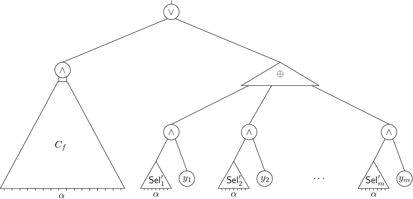
Figure 1: A schematic depiction of the formula after hitting it with the described restriction.

Note that this implements the intended semantics: for each input $\alpha\in\{0,1\}^{n}$ the selector circuits output $1$ on some variables $y_{i}$ which are then xor’ed, and the restricted circuit outputs

$$\bigoplus_{i\in N(\alpha)}y_{i}\enspace,$$ (16)

unless $C_{f}(\alpha)\neq\bot$, in which case the output of the circuit is $f(\alpha)$ and all selector circuits output $0$. We require that $s$ is larger than the size of the described circuit which is of size $O\big{(}m\cdot\poly(n,k)\big{)}+s/2$.

We have the intended semantics of the circuit and need to ensure the furthermore property: that the restricted formula is over few variables. First, since the selector circuits $\operatorname{\mathsf{Sel}}^{\prime}_{i}$ are fixed, all evaluation variables for these subcircuits can be fixed to constants. The same holds for the circuit $C_{f}$. Similarly, since the $y_{i}$ gate always carries the value of the $y_{i}$ variable, all $2^{n}\cdot m$ wire variables corresponding to the $Y$ variables can be substituted by the corresponding $y_{i}$ variable and are thus restricted away.

After these restrictions the only evaluation variables left are those for the evaluation of the $\oplus$ circuit. For $\alpha$ such that $C_{f}(\alpha)\neq\bot$, the selector circuits are hard-wired to $0$ and in particular the inputs to the $\oplus$ circuit is hard-wired to $0$, meaning that these evalation variables can be restricted away.

There remains then only the $O(t\cdot m)$ evaluation variables corresponding to the evaluation of the $\oplus$ circuit for inputs $\alpha$ such that $C_{f}(\alpha)=\bot$. Let us, without loss of generality, use an xor-circuit which iteratively xors each variable. Concretely, let it have subcircuits $\chi_{i}$ where $\chi_{1}=\operatorname{\mathsf{Sel}}^{\prime}_{1}\wedge y_{1}$ and $\chi_{i}=\chi_{i-1}\oplus(\operatorname{\mathsf{Sel}}^{\prime}_{i}\wedge y_{i})$ for $i>1$, and $\chi_{m}$ is the overall output of the $\oplus$ circuit.

The only observation required is that if the circuit $\operatorname{\mathsf{Sel}}^{\prime}_{i}(\alpha)=0$, then $\chi_{i}$ gets a $0$ as input from index $i$, independent of the value of $y_{i}$. Hence the output wire variable of the circuit $\chi_{i}$ indexed by the input $\alpha$ can be substituted by the output of the circuit $\chi_{i-1}$. Hence for each $\alpha$ such that $C_{f}(\alpha)=\bot$, we can reduce the number of free wire variables indexed by $\alpha$ to $O(k)$, as each $\oplus$-constraint is over at most $k$ variables. As $C_{f}$ outputs $\bot$ on at most $t$ inputs, we end up with a restriction leaving only a total of $O(t\cdot k+m)$ remaining variables in the restricted formula.

This completes the description of the restriction $\rho$. The only part that remains is to verify that $\rho$ is natural, $k$-determined, and $m$-independent. That $\rho$ is natural is immediate – it does not substitute any structural variable by an evaluation variable. For $k$-determinedness, note that for a fixed input $\alpha$ at most $k$ selector circuits output $1$, and thus for every gate $u$ the value of $\operatorname{\mathsf{Out}}_{\alpha}(u)$ as a function of $Y$ can be computed by a function over those $k$ variables. Finally, each assignment to the remaining structure variables $Y$ gives a valid circuit and thus $\rho$ is $m$-independent. ∎

We are ready to prove the degree lower bound, restated here for convenience.

See 1.1

Proof.

Let $G=(U,V,E)$ be an explicit bipartite graph as in Theorem 2.3, with $U=\{0,1\}^{n}$, $k=O_{\gamma}\big{(}(n\log r)^{1+1/\gamma}\big{)}$, and $|V|\leq k^{2}r^{1+\gamma}$ for parameters $\gamma>0$ and $r\leq 2^{n}$ to be fixed later. Apply Lemma 4.1 with $t=2^{n}$ along with $C_{f}=\bot$ to obtain, for $s\geq m\cdot\poly(n,k)$, a natural $m$-independent $k$-determined variable substitution $\rho$ for $\operatorname{Circuit}_{s}(f)$ such that $g^{\mathrm{out}}_{s,\alpha}(Y)=\oplus_{i\in N(\alpha)}y_{i}$. In words, the circuit of the restricted formula on input $\alpha$ computes an xor of the neighborhood of the vertex $\alpha$ of $G$.

Apply Lemma 3.4 to $\rho$ to conclude that if there is an SoS refutation of ${\left.\kern-1.2pt\operatorname{Circuit}_{s}(f)\vphantom{\big{|}}\right|_{\rho}}$ of degree $d$, then there is a degree $d\cdot k$ SoS refutation of the system of polynomial equations computing

$$\mathcal{P}_{G} =\Big{\{}\bigoplus_{i\in N(\alpha)}y_{i}=f(\alpha):\alpha\in\{0,1\}^{n}\Big{\}}\,\cup\{y_{i}^{2}=y_{i}\mid i\in[m]\}\enspace.$$

As the graph $G$ is a strong expander, we can apply Theorem 2.8 to get an SoS degree lower bound of $\Omega(r)$ for the XOR-CSP instance $\mathcal{P}_{G}$ defined over $G$, which in turn gives us an $\Omega(r/k)$ degree lower bound for the ${\left.\kern-1.2pt\operatorname{Circuit}_{s}(f)\vphantom{\big{|}}\right|_{\rho}}$ formula and hence also for the unrestricted formula.

Let us fix the parameters. We want to choose $r$ as large as possible. However, the larger we choose $r$, the larger $m$ may become, since Theorem 2.3 only guarantees that $m\leq k^{2}r^{1+\gamma}$. Let us analyze how large $r$ can be chosen in terms of $n$ and $s$.

Note that $k=\poly_{\gamma}(n)$, where we use that $r\leq 2^{n}$, and we write $\poly_{\gamma}(n)$ to denote some polynomial in $n$ whose degree and coefficients may depend on $\gamma$. Hence we may choose

$$m=\frac{s}{\poly_{\gamma}(n)}\enspace,$$ (17)

according to the requirement on $s$ in Lemma 4.1. From the guarantees of Theorem 2.3 we know that $r\geq(m/k^{2})^{1/(1+\gamma)}$. Substituting $m$ according to the previous equation we get that

$$r\geq\left(\frac{s}{k^{2}\poly_{\gamma}(n)}\right)^{\frac{1}{1+\gamma}}=\frac{s^{1/(1+\gamma)}}{\poly_{\gamma}(n)}\enspace.$$ (18)

Hence if we choose $\gamma$ small enough so that $\frac{1}{1+\gamma}>1-\varepsilon/2$ and then require $s$ to be large enough such that the final $\poly_{\gamma}(n)$ is at most $s^{\varepsilon/2}$, we obtain the claimed lower bound. ∎

In the following we prove the claimed size lower bound.

See 1.3

Proof.

Apply Lemma 4.1 with the graphs from Theorem 2.3 as in the proof of Theorem 1.1. We get a natural $m$-independent $k$-determined variable substitution $\rho$ and the formula ${\left.\kern-1.2pt\operatorname{Circuit}_{s}(f)\vphantom{\big{|}}\right|_{\rho}}$ over $O(t\cdot k+m)$ variables. To this formula we then apply Lemma 3.4 to obtain a degree lower bound of $\Omega(r/k)$, akin to the proof of Theorem 1.1. By setting the parameters as in the aforementioned proof we get the same degree lower bound of $\Omega_{\varepsilon}(s^{1-\varepsilon/3})$ for the formula ${\left.\kern-1.2pt\operatorname{Circuit}_{s}(f)\vphantom{\big{|}}\right|_{\rho}}$. As this formula is over few variables we can apply Theorem 2.9 to obtain an SoS size lower bound of $\exp\Big{(}\Omega_{\varepsilon}\big{(}(s^{1-\varepsilon/3}-3k)^{2}/(t\cdot k+m)\big{)}\Big{)}$ for the restricted formula. As variable substitutions may only decrease the size of a refutation, the same lower bound also holds for the unrestricted formula. We obtain the desired lower bound by choosing $s$ large enough such that $s^{\varepsilon/3}\geq k=\poly_{\varepsilon}(n)$ and by recalling that $t\geq s\geq m$. ∎

5 Lower Bounds for Monotone Circuits

Recall that $\mathcal{M}_{n}(\ell)$ denotes all Boolean monotone $\ell$-slice functions on $n$ bits: all Boolean functions $f:\{0,1\}^{n}\rightarrow\{0,1\}$ that output $0$ on all inputs of Hamming weight less than $\ell$ and $1$ on all inputs of Hamming weight larger than $\ell$. There is no restriction on the output for inputs of Hamming weight $\ell$ and we have $|\mathcal{M}_{n}(\ell)|=2^{\binom{n}{\ell}}$. Further, recall that $\mathcal{M}_{n}(\ell,s,t)\subseteq\mathcal{M}_{n}(\ell)$ is the class of monotone Boolean $\ell$-slice functions $f:\{0,1\}^{n}\rightarrow\{0,1\}$ for which there is a (not necessarily monotone) Boolean circuit $C_{f}^{\mathsf{mon}}:\{0,1\}^{n}\rightarrow\{0,1,\bot\}$ of size $s$ such that

1. for all $\ell$-slice inputs $\alpha\in\binom{[n]}{\ell}$ it holds that if $C^{\mathsf{mon}}_{f}(\alpha)\neq\bot$, then $C^{\mathsf{mon}}_{f}(\alpha)=f(\alpha)$, and

2. $C^{\mathsf{mon}}_{f}(\alpha)=\bot$ on at most $t$ inputs $\alpha\in\binom{[n]}{\ell}$.

It is very convenient to work with slice functions as we have a handle on their monotone circuit complexity: by Lemma 2.5 their monotone circuit size is the same as their ordinary circuit size up to a polynomial size increase. Hence we do not need to worry whether the functions needed for the reduction have small monotone circuits, as long as we are working on a slice only.

The proof of the monotone lower bound is an adaption of the argument used to prove Lemma 4.1. The idea is to work over the $\ell$th slice and disregard all other inputs. By Lemma 2.5 we can implement our selector circuits by small monotone circuits. We then also need to take care of the negations in the $\oplus$-circuit. We push the negations down until they either hit a gate in $Y$ or a selector circuit. We create a set $\overline{Y}$ gates, which we can think of as the negation of the gates in $Y$ and also create negated selector circuits (on the $\ell$th slice). By doing so we can now get rid of the last negations by appropriately connecting the appropriate circuits. The following corollary of Lemma 2.5 will be useful to us.

Claim 5.1.

Let $C$ be a Boolean circuit on $n$ input bits of size $s$. Then, for $\ell\in[n]$, there is a monotone Boolean circuit $C^{\mathsf{mon}}$ of size $2s+\poly(n)$ computing the $\ell$-slice function that is equal to $C$ on the $\ell$-slice.

Proof.

Let $\mathcal{T}_{\geq\ell}$ be the threshold function that outputs $1$ if and only if the Hamming weight of an input $\alpha\in\{0,1\}^{n}$ is at least $\ell$. Connect the output of $C$ by an and gate to a circuit computing $\mathcal{T}_{\geq\ell}$. The output of this circuit is then connected by an or gate to the output of a circuit computing $\mathcal{T}_{>\ell}$. Let us denote this new circuit by $C^{\prime}$.

The circuit $C^{\prime}$ clearly outputs $1$ whenever the input is of Hamming weight larger than $\ell$. Furthermore, on the $\ell$-slice it is equal to $C$ because $\mathcal{T}_{\geq\ell}$ outputs $1$ while $\mathcal{T}_{>\ell}$ outputs $0$. Finally the output is $0$ if the Hamming weight is less than $\ell$ because the output of both threshold functions is $0$.

Clearly the size of the circuits computing the threshold functions is $\poly(n)$. We apply Lemma 2.5 to conclude that there is a monotone circuit $C^{\mathsf{mon}}$ computing the same function as $C^{\prime}$ of size $2s+\poly(n)$. ∎

Before stating the following lemma we need to adapt some terminology to the monotone setting. Observe that $\operatorname{Circuit}_{s}^{\mathsf{mon}}(f)$ is a restriction of $\operatorname{Circuit}_{s}(f)$. Let $\tau$ be such that ${\left.\kern-1.2pt\operatorname{Circuit}_{s}(f)\vphantom{\big{|}}\right|_{\tau}}=\operatorname{Circuit}^{\mathsf{mon}}_{s}(f)$. This allows us to naturally extend $k$-determined restrictions to the monotone setting: a restriction $\rho$ is a $k$-determined restriction for $\operatorname{Circuit}^{\mathsf{mon}}_{s}(f)$ if the restriction $\rho\tau$ is a $k$-determined restriction for $\operatorname{Circuit}_{s}(f)$. Similarly we can extend $m$-independence to the monotone setting. This will later allow us to use Lemma 3.4 even though we are working with the monotone formula.

Lemma 5.2.

For all $k,\ell,m,n,t\in\mathbb{N}$ satisfying $m\leq 2^{n}$, and any explicit bipartite graph $G=(U,V,E)$ such that $|U|=2^{n}$, $|V|=m$ and all $u\in U$ are of degree $\deg(u)\leq k$, the following holds. There is a constant $C>0$, depending on the explicitness of $G$, such that for all $s\geq C\cdot m\cdot n^{C}\cdot k^{C}$ and any $f\in\mathcal{M}_{n}(\ell,s/10,t)$ there is a natural $m$-independent $k$-determined variable substitution $\rho$ for the formula $\operatorname{Circuit}^{\mathsf{mon}}_{s}(f)$ such that

$$g^{\mathrm{out}}_{s,\alpha}(Y)=\begin{cases}1,&\text{if\leavevmode\nobreak\ }|\alpha|>\ell,\\ 0,&\text{if\leavevmode\nobreak\ }|\alpha|<\ell,\\ f(\alpha),&\text{if\leavevmode\nobreak\ }|\alpha|=\ell\text{\leavevmode\nobreak\ and\leavevmode\nobreak\ }C_{f}^{\mathsf{mon}}(\alpha)\neq\bot,\\ \oplus_{i\in N(\alpha)}y_{i},&\text{otherwise},\\ \end{cases}$$

for $g^{\mathrm{out}}_{s,\alpha}$ and $Y$ as in Definition 3.2.

Furthermore, the formula ${\left.\kern-1.2pt\operatorname{Circuit}^{\mathsf{mon}}_{s}(f)\vphantom{\big{|}}\right|_{\rho}}$ is over $O(t\cdot k+m)$ variables.

Proof.

This proof is an adaptation of the argument of the proof Lemma 4.1. Let us describe the natural $m$-independent $k$-determined restriction $\rho$ for the formula $\operatorname{Circuit}_{s}^{\mathsf{mon}}(f)$.

As in the proof of Lemma 4.1 we have gates that act as Boolean variables. But instead of having a single set $Y$ of variables we now have two sets $Y$ and $\overline{Y}$, each of size $m$. We think of the variables in $\overline{Y}$ as the negations of the variables in $Y$ and ensure this by applying the appropriate variable substitution for all $\alpha\in\{0,1\}^{n}$ and $i\in[m]$.

According to 5.1 we may assume that the circuit $C_{f}^{\mathsf{mon}}$ computes a monotone $\ell$-slice function in both outputs $C_{f,1}^{\mathsf{mon}},C_{f,2}^{\mathsf{mon}}$ for a mild increase in size; $|C_{f}^{\mathsf{mon}}|\leq s/5+\poly(n)\leq s/4$ for $s$ large enough. Recall that the first output of $C_{f}^{\mathsf{mon}}$ indicates whether the second output bit is equal to $f$ on the $\ell$-slice. Let $\overline{C}^{\mathsf{mon}}_{f,1}$ be the negation of $C_{f,1}^{\mathsf{mon}}$ on the $\ell$-slice. In other words, $\overline{C}^{\mathsf{mon}}_{f,1}(\alpha)=\lnot C_{f,1}^{\mathsf{mon}}(\alpha)$ if $\alpha$ has Hamming weight $\ell$, and $\overline{C}^{\mathsf{mon}}_{f,1}(\alpha)=C_{f,1}^{\mathsf{mon}}(\alpha)$ otherwise.

The monotone circuit $C_{f}^{\mathsf{mon}}$ is of size at most $s/4$ and hence according to Lemma 2.5 there is a monotone circuit of size $s/2+\poly(n)\leq 5s/8$ computing $\overline{C}^{\mathsf{mon}}_{f,1}(\alpha)$.

We restrict the formula such that a part of the circuit is equivalent to $C_{f}^{\mathsf{mon}}$ and another part is equal to $\overline{C}^{\mathsf{mon}}_{f,1}$. Note that the size of these two circuits is at most $7s/8$ by above discussion.

Recall that because $G(\{0,1\}^{n},Y,E)$ is explicit, there are circuits $\operatorname{\mathsf{Sel}}_{1},$ $\operatorname{\mathsf{Sel}}_{2},\ldots,\operatorname{\mathsf{Sel}}_{m}$, each of size $\poly(n,k)$, where each $\operatorname{\mathsf{Sel}}_{i}$ computes, given an input $\alpha\in\{0,1\}^{n}$, whether the vertex $y_{i}\in Y$ is a neighbor of the vertex $\alpha$. Let $\overline{\operatorname{\mathsf{Sel}}}_{i}=\lnot\operatorname{\mathsf{Sel}}_{i}$ and denote by $\operatorname{\mathsf{Sel}}_{i}^{\mathsf{mon}}$ (respectively $\overline{\operatorname{\mathsf{Sel}}}_{i}^{\mathsf{mon}}$) the circuit obtained by applying 5.1 to $\operatorname{\mathsf{Sel}}_{i}$ (to $\overline{\operatorname{\mathsf{Sel}}}_{i}$ respectively). By the guarantees of 5.1 all these $2m$ circuits are of size $\poly(n,k)$.

We restrict the formula such that a part of the circuit computes the functions

$$\operatorname{\mathsf{Sel}}_{1}^{\mathsf{mon}},\ldots,\operatorname{\mathsf{Sel}}^{\mathsf{mon}}_{m},\overline{\operatorname{\mathsf{Sel}}}^{\mathsf{mon}}_{1},\ldots,\overline{\operatorname{\mathsf{Sel}}}^{\mathsf{mon}}_{m}\enspace.$$ (19)

From these $\ell$-slice selector circuits we can then define selector circuits that take $C_{f}^{\mathsf{mon}}$ into account. Namely, we connect $\operatorname{\mathsf{Sel}}_{i}^{\mathsf{mon}}$ by an and gate to the output of $\overline{C}_{f,1}^{\mathsf{mon}}$ to obtain the circuit $\operatorname{\mathsf{Sel}}_{i}^{\prime{\mathsf{mon}}}$ and similarly connect $\overline{\operatorname{\mathsf{Sel}}}^{\mathsf{mon}}_{i}$ by an or gate to $C_{f,1}^{\mathsf{mon}}$ to obtain the circuit $\overline{\operatorname{\mathsf{Sel}}}_{i}^{\prime{\mathsf{mon}}}$.

Finally, we also put each variable $y_{i}$ and $\bar{y}_{i}$ onto the slice by the same construction used in the proof of 5.1: connect the variable $y_{i}$ (respectively $\bar{y}_{i}$) by an and to the threshold circuit $\mathcal{T}_{\geq\ell}$ and connect this circuit in turn by an or gate to a $\mathcal{T}_{>\ell}$ threshold circuit to obtain $y_{i}^{\mathsf{mon}}$ (respectively $\bar{y}_{i}^{\mathsf{mon}}$). It is well-known [Val84, BW06, Gol20] that threshold circuits have montone circuits of size $\poly(n)$ and we can thus restrict the formula such that a part of the circuit computes $y_{i}^{\mathsf{mon}}$ and $\bar{y}_{i}^{\mathsf{mon}}$.

Finally we connect $y^{\mathsf{mon}}_{i}$ by an and gate to the selector circuit $\operatorname{\mathsf{Sel}}_{i}^{\prime{\mathsf{mon}}}$. Note that this circuit is equal to an $\ell$-slice function. As we will see later this ensures that the whole circuit outputs an $\ell$-slice function. We connect the circuits $\bar{y}^{\mathsf{mon}}_{i}$ similarly: connect $\bar{y}^{\mathsf{mon}}_{i}$ by an or gate to the negated selector circuit $\overline{\operatorname{\mathsf{Sel}}}_{i}^{\prime{\mathsf{mon}}}$. Again, the output of this circuit is equal to an $\ell$-slice function.

Equally inportant is that these circuits behave well on the $\ell$-slice. Indeed it can be checked that the positive circuit, on input $\alpha\in\{0,1\}^{n}$, outputs $\operatorname{\mathsf{Sel}}_{i}^{\prime{\mathsf{mon}}}(\alpha)\land y_{i}$ while the negative circuit outputs $\overline{\operatorname{\mathsf{Sel}}}_{i}^{\prime{\mathsf{mon}}}(\alpha)\lor\bar{y}_{i}$. On the $\ell$-slice these functions are the negation of eachother, which we are going to use in the following.

We need to construct a monotone circuit for the xor of $\operatorname{\mathsf{Sel}}_{i}^{\prime{\mathsf{mon}}}(\alpha)\wedge y_{i}$ for $i$ from $1$ to $m$, on $\ell$-slice inputs $\alpha$. We take a standard $O(m)$-size $\oplus$-circuit and monotonize it by pushing all negations in it down using De Morgan’s law until they reach one of the $\oplus$-circuit’s inputs $\operatorname{\mathsf{Sel}}_{i}^{\prime{\mathsf{mon}}}\wedge y_{i}$. Whenever the negation of $\operatorname{\mathsf{Sel}}_{i}^{\prime{\mathsf{mon}}}(\alpha)\wedge y_{i}$ is needed, we do one last step of De Morgan and replace it by $\overline{\operatorname{\mathsf{Sel}}}_{i}^{\prime{\mathsf{mon}}}(\alpha)\vee\bar{y}_{i}$.

To ensure that the circuit outputs $f(\alpha)$ whenever $C^{\mathsf{mon}}_{f}(\alpha)\neq\bot$, we connect the two outputs of $C_{f}^{\mathsf{mon}}$ by an and gate and connect this gate by an or gate to the output of the xor circuit. This completes the description of the restriction on the structure variables. A depiction of the resulting circuit can be found in Figure 2.

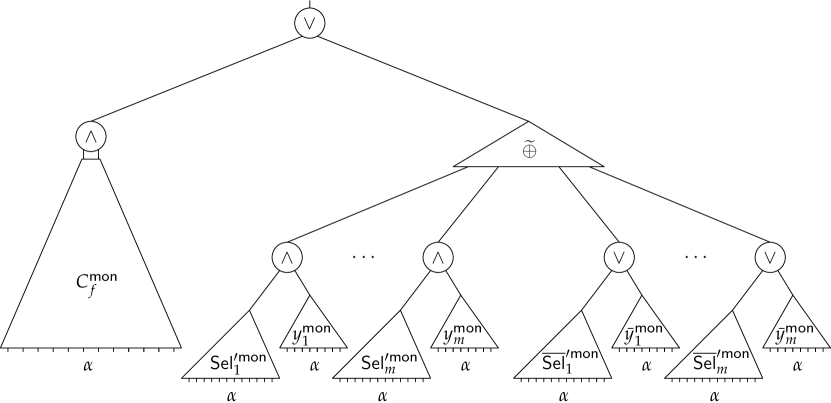
Figure 2: A depiction of the monotone circuit, where $\widetilde{\oplus}$ is the $\oplus$ circuit with the negations pushed down.

We ensure that $s$ is large enough so that above circuit can be described by the formula.

Note that the constructed circuit always outputs a monotone $\ell$-slice function: as the monotonized $\oplus$-circuit is non-constant, we see that if all inputs to the circuit are $0$, it outputs $0$ and if all inputs are $1$, it outputs $1$. This, in particular, implies that the circuit outputs $0$ (respectively $1$) if the input is below (respectively, above) the $\ell$-slice and hence the entire circuit computes a monotone $\ell$-slice function.

It can be easily checked that the described restriction is $m$-independent and $k$-determined. In order to prove the furthermore part, we need to reduce the number of evaluation variables. This can be achieved analogous to the proof of Lemma 4.1 and we thus omit it here. ∎

Let us prove our degree lower bound for monotone circuits, restated here for convenience.

See 1.4

Proof of Theorem 1.4.

As in the proof of Theorem 1.1, we use the graphs from Theorem 2.3, with $U=\{0,1\}^{n}$, $k=O_{\gamma}\big{(}(n\log r)^{1+1/\gamma}\big{)}$, and $|V|\leq k^{2}r^{1+\gamma}$ for parameters $\gamma>0$ and $r\leq 2^{n}$. We apply Lemma 5.2 with above graph and $t=2^{n}$ along with $C_{f}^{\mathsf{mon}}=\bot$ to obtain, for $s\geq m\cdot\poly(n,k)$, an appropriate natural $m$-independent $k$-determined variable substitution $\rho$ for $\operatorname{Circuit}^{\mathsf{mon}}_{s}(f)$. In particular $\rho$ satisfies

$$g^{\mathrm{out}}_{s,\alpha}(Y)=\begin{cases}1,&\text{if\leavevmode\nobreak\ }|\alpha|>\ell,\\ 0,&\text{if\leavevmode\nobreak\ }|\alpha|<\ell,\\ \oplus_{i\in N(\alpha)}y_{i},&\text{otherwise},\\ \end{cases}$$

for $g^{\mathrm{out}}_{s,\alpha}$ and $Y$ as in definition Definition 3.2.

Recall that there is a restriction $\tau$ such that $\operatorname{Circuit}_{s}^{\mathsf{mon}}(f)={\left.\kern-1.2pt\operatorname{Circuit}_{s}(f)\vphantom{\big{|}}\right|_{\tau}}$ and we can thus apply Lemma 3.4 with $\tau\rho$ to conclude that if there is an SoS refutation of ${\left.\kern-1.2pt\operatorname{Circuit}^{\mathsf{mon}}_{s}(f)\vphantom{\big{|}}\right|_{\rho}}$ in degree $d$, then there is a degree $d\cdot k$ SoS refutation of the system of polynomial equations computing

$$\{\bigoplus_{i\in N(\alpha)}y_{i}=f(\alpha)\mid\alpha\in\binom{[n]}{\ell}\}\enspace.$$ (20)

As the graph $G$ is a strong expander, we can apply Theorem 2.8 to get an SoS degree lower bound of $\Omega(r)$ for above system of equations. By above connection this gives an $\Omega(r/k)$ degree lower bound for the ${\left.\kern-1.2pt\operatorname{Circuit}^{\mathsf{mon}}_{s}(f)\vphantom{\big{|}}\right|_{\rho}}$ formula and hence also for the unrestricted formula.

Regarding the parameters, as in the proof of Theorem 1.1 we choose $m=s/\poly_{\gamma}(n)$. Repeating the calculations from the aforementioned proof we obtain that $r\geq s^{1/(1+\gamma)}/\poly_{\gamma}(n)$. Thus by choosing $\gamma$ small enough such that $\frac{1}{1+\gamma}>1-\varepsilon/2$ and $s$ large enough such that the final $\poly_{\gamma}(n)\leq s^{\varepsilon/2}$ we obtain the claimed degree lower bound of $\Omega_{\varepsilon}(s^{1-\varepsilon})$. ∎

As in the non-monotone case, we can also obtain size lower bounds for functions that almost have a circuit of size $s$.

See 1.5

Proof.

Analogous to the proof of Theorem 1.3. ∎

6 Degree Upper Bound

In this section we give a simple upper bound on the SoS refutation degree for $\operatorname{Circuit}_{s}(f)$. Specifically, for functions $f$ that have no circuit of size $s$, we show that there is an SoS refutation of $\operatorname{Circuit}_{s}(f)$ of degree $O(s)$, essentially matching our $\Omega(s^{1-\epsilon})$ lower bound.

At a high level, the logic behind the refutation is as follows: first, we show that SoS in degree $O(s)$ can derive that the $\Theta(s^{2})$ structure variables of $\operatorname{Circuit}_{s}(f)$ must uniquely describe a circuit of size $s$. Then, we also show that for any fixed circuit, SoS can in degree $O(s)$ derive that the circuit does not compute $f$ by “evaluating” the circuit on some (non-deterministically chosen) input where the output differs from $f$.

To make this precise, we first define a set of monomials, which correspond to circuits of size $s$. A multilinear monomial $m$ is a circuit monomial if for every gate $v\in[s]$ it holds that

1. exactly one of the variables $\operatorname{\mathsf{IsNeg}}(v),\operatorname{\mathsf{IsOr}}(v)$ or $\operatorname{\mathsf{IsAnd}}(v)$ occurs in $m$,

2. for $a\in\{1,2\}$ exactly one of the variables $\operatorname{\mathsf{IsFromConst}}(v,a)$, $\operatorname{\mathsf{IsFromInput}}(v,a)$ or $\operatorname{\mathsf{IsFromGate}}(v,a)$ occurs in $m$,

3. for $a\in\{1,2\}$ exactly one of the variables $\operatorname{\mathsf{ConstantValue}}(v,a)$ or $\overline{\operatorname{\mathsf{ConstantValue}}(v,a)}$ occurs in $m$,

4. for $a\in\{1,2\}$ exactly one of the variables $\{\operatorname{\mathsf{IsInput}}(v,a,i)\mid i\in[n]\}$ occurs in $m$, and

5. for $a\in\{1,2\}$ and $v>1$, exactly one of the variables $\{\operatorname{\mathsf{IsGate}}(v,a,u)\mid u<v\}$ occurs in $m$, and

6. no other variables occur in $m$ than the ones described above.

We denote by $\mathcal{M}_{s}$ the set of circuit monomials. We first show that SoS can derive in degree $O(s)$ the polynomial $\sum_{m\in\mathcal{M}_{s}}m-1$; this corresponds to SoS proving that the structure variables uniquely describe a circuit and does not use anything about $f$. Then in a second step we show that for every $m\in\mathcal{M}_{s}$, SoS can derive $-m$ in degree $O(s)$; this corresponds to SoS proving that the circuit described by $m$ does not compute $f$ correctly. Summing these two parts up yields an SoS derivation of $-1$, i.e., a refutation of the $\operatorname{Circuit}_{s}(f)$ formula.

Deriving $\bm{\sum_{m\in\mathcal{M}_{s}}m-1}$.

We proceed by induction on $s$. Note that $\mathcal{M}_{0}=\{1\}$ and hence the base case is trivial. Suppose we have an SoS derivation of $\sum_{m\in\mathcal{M}_{s}}m-1$. For every monomial $m\in\mathcal{M}_{s}$ we add the polynomial

$$m\cdot\big{(}\operatorname{\mathsf{IsNeg}}(v)+\operatorname{\mathsf{IsOr}}(v)+\operatorname{\mathsf{IsAnd}}(v)-1\big{)}$$ (21)

to the derivation (note that the second term is Equation 2). This gives us an SoS derivation of $\sum_{m\in\mathcal{M}^{\prime}_{s}}m-1$, where

$$\mathcal{M}^{\prime}_{s}=\bigcup_{m\in\mathcal{M}_{s}}\{m\cdot\operatorname{\mathsf{IsNeg}}(v),m\cdot\operatorname{\mathsf{IsOr}}(v),m\cdot\operatorname{\mathsf{IsAnd}}(v)\}\enspace.$$

We can continue in the same manner with Equation 1 and Equation 3 to finally obtain an SoS derivation of $\sum_{m\in\mathcal{M}_{s+1}}m-1$. Clearly this derivation requires degree at most $O(s)$, as for each gate there are at most $7$ variables in every monomial from $\mathcal{M}_{s}$.

Deriving $-m$ for $m\in\mathcal{M}_{s}$.

Let $C$ be the circuit that corresponds to the monomial $m$ and let $\alpha\in\{0,1\}^{n}$ be such that $f(\alpha)\neq C(\alpha)$ (by the assumption that $f$ does not have a circuit of size $s$, such an $\alpha$ exists). Suppose $C(\alpha)=b$ but $f(\alpha)=1-b$.

We construct a degree $O(s)$ SoS proof of the fact that $C(\alpha)=b$. That is, we are going to show that the polynomial $p_{s}=m\cdot\left(\operatorname{\mathsf{Out}}_{\alpha}(s)-b\right)$ can be written as

$$p_{s}=\sum_{i=1}^{t}r_{i}\cdot q_{i}\enspace,$$ (22)

for some parameter $t$, axioms $q_{1},\ldots,q_{t}$ and some polynomials $r_{1},\ldots,r_{t}$, such that $\deg(r_{i}\cdot q_{i})=O(s)$ for all $i$. Note that given this, we can then easily derive $-m$ by subtracting the polynomial $m\cdot\left(\operatorname{\mathsf{Out}}_{\alpha}(s)-f(\alpha)\right)=m\cdot\left(\operatorname{\mathsf{Out}}_{\alpha}(s)-1+b\right)$ (this is $m$ multiplied by Equation 13), yielding a derivation of $m\cdot(1-2b)$ which is either $m$ or $-m$ depending on $b$; in the former case it can be multiplied by $-1$ to yield $-m$. Note that here it is important that the derivation (22) is a Nullstellensatz derivation, not using any Sum-of-Squares part, since otherwise it would not be possible to multiply it by $-1$.

Let us thus see how to derive $m\cdot\left(\operatorname{\mathsf{Out}}_{\alpha}(s)-b\right)$. We do this by structural induction over the circuit: for every gate $v$ we are going to construct an SoS proof of the fact that the circuit rooted at $v$ outputs the bit $b_{v}$ on input $\alpha$. In other words, an SoS derivation of the polynomial $m\cdot\left(\operatorname{\mathsf{Out}}_{\alpha}(v)-b_{v}\right)$.

Let us explain how to construct an SoS proof $p_{v}$. Consider a gate $v$ in the circuit. Depending on the function computed at $v$ and how the wires of $v$ are connected we construct $p_{v}$ slightly differently. As a first step let us construct SoS proofs $q_{1}$ and $q_{2}$ of the fact that on input $\alpha$ the bit $c_{a}$, $a\in\{1,2\}$, is carried on wire $a$ to the gate $v$. That is, the polynomial $q_{a}$ should simplify to $m\cdot\big{(}\operatorname{\mathsf{In}}_{\alpha}(v,a)-c_{a}\big{)}$. In the following we explain how to precisely define $q_{a}$ depending on what the wire is connected to. Note that not a lot is going on – we are mostly just multilinearizing using the Boolean axioms.

If $m$ is of the form $m=m^{\prime}\cdot\operatorname{\mathsf{IsFromConst}}(v,a)\cdot\operatorname{\mathsf{ConstantValue}}(v,a)$ for some monomial $m^{\prime}$, i.e., wire $a$ is connected to the constant $c_{a}=1$ in the circuit described by $m$, then we can derive $q_{a}=m\cdot\big{(}\operatorname{\mathsf{In}}_{\alpha}(v,a)-1\big{)}$ by the identity

$$q_{a} =m^{\prime}\cdot\operatorname{\mathsf{ConstantValue}}(v,a)\cdot\operatorname{\mathsf{IsFromConst}}(v,a)\cdot\big{(}\operatorname{\mathsf{In}}_{\alpha}(v,a)-\operatorname{\mathsf{ConstantValue}}(v,a)\big{)}+$$

$$\qquad m^{\prime}\cdot\operatorname{\mathsf{IsFromConst}}(v,a)\cdot\big{(}\operatorname{\mathsf{ConstantValue}}(v,a)^{2}-\operatorname{\mathsf{ConstantValue}}(v,a)\big{)}\enspace,$$ (23)

a linear combination of Equation 7 and the Boolean axiom on $\operatorname{\mathsf{ConstantValue}}(v,a)$. Similarly if $m=m^{\prime}\cdot\operatorname{\mathsf{IsFromConst}}(v,a)\cdot\overline{\operatorname{\mathsf{ConstantValue}}(v,a)}$ (i.e., $c_{a}=0$) we can derive $q_{a}=m\cdot\operatorname{\mathsf{In}}_{\alpha}(v,a)$ by

$$q_{a} =m^{\prime}\cdot\overline{\operatorname{\mathsf{ConstantValue}}(v,a)}\cdot\operatorname{\mathsf{IsFromConst}}(v,a)\cdot\big{(}\operatorname{\mathsf{In}}_{\alpha}(v,a)-\operatorname{\mathsf{ConstantValue}}(v,a)\big{)}+$$

$$\qquad m^{\prime}\cdot\operatorname{\mathsf{IsFromConst}}(v,a)\cdot\operatorname{\mathsf{ConstantValue}}(v,a)\cdot$$

$$\qquad\qquad\qquad\big{(}1-\operatorname{\mathsf{ConstantValue}}(v,a)-\overline{\operatorname{\mathsf{ConstantValue}}(v,a)}\big{)}+$$

$$\qquad m^{\prime}\cdot\operatorname{\mathsf{IsFromConst}}(v,a)\cdot(\operatorname{\mathsf{ConstantValue}}(v,a)^{2}-\operatorname{\mathsf{ConstantValue}}(v,a))\enspace,$$ (24)

where we additionally use the negation axiom on $\operatorname{\mathsf{ConstantValue}}(v,a)$.

Next, if $a$ is connected to an input $i$ and $m$ is of the form $m=m^{\prime}\cdot\operatorname{\mathsf{IsFromInput}}(v,a)\cdot\operatorname{\mathsf{IsInput}}(v,a,i)$ (so that $c_{a}=\alpha_{i}$), then

$$q_{a}=m\cdot(\operatorname{\mathsf{In}}_{\alpha}(v,a)-\alpha_{i}) =m^{\prime}\cdot\operatorname{\mathsf{IsFromInput}}(v,a)\cdot\operatorname{\mathsf{IsInput}}(v,a,i)\cdot\big{(}\operatorname{\mathsf{In}}_{\alpha}(v,a)-\alpha_{i}\big{)}\enspace,$$ (25)

which is a multiple of Equation 8. Lastly, if $a$ is connected to a gate $u$ and $m$ is of the form $m=m^{\prime}\cdot\operatorname{\mathsf{IsFromGate}}(v,a)\cdot\operatorname{\mathsf{IsGate}}(v,a,u)$ (i.e., $c_{a}=b_{u}$), then

$$q_{a}=m\cdot(\operatorname{\mathsf{In}}_{\alpha}(v,a)-b_{u}) =m^{\prime}\cdot\operatorname{\mathsf{IsFromGate}}(v,a)\cdot\operatorname{\mathsf{IsGate}}(v,a,u)\cdot\big{(}\operatorname{\mathsf{In}}_{\alpha}(v,a)-\operatorname{\mathsf{Out}}_{\alpha}(u)\big{)}$$

$$\qquad+m\cdot(\operatorname{\mathsf{Out}}_{\alpha}(u)-b_{u})\enspace,$$ (26)

where the first term is a multiple of Equation 9, and the second term is the polynomial $p_{u}$ which, by induction, we assume has already been derived in degree $O(s)$.

Given the two SoS proofs $q_{1}$ and $q_{2}$ we are ready to construct the SoS proof $p_{v}=m\cdot(\operatorname{\mathsf{Out}}_{\alpha}(v)-b_{v})$. As mentioned earlier we do a case distinction over the funtion computed at $v$.

1. $v$ is a not gate ($m=m^{\prime}\cdot\operatorname{\mathsf{IsNeg}}(v)$ and $b_{v}=1-c_{1}$). We have the derivation

   $$p_{v} =m^{\prime}\cdot\operatorname{\mathsf{IsNeg}}(v)\cdot\big{(}\operatorname{\mathsf{Out}}_{\alpha}(v)-\overline{\operatorname{\mathsf{In}}_{\alpha}(v,1)}\big{)}$$

   $$\qquad+m\cdot\big{(}\overline{\operatorname{\mathsf{In}}_{\alpha}(v,1)}-1+\operatorname{\mathsf{In}}_{\alpha}(v,1)\big{)}$$

   $$\qquad-q_{1}\enspace,$$ (27)

   where the first line uses Equation 10 and the second line uses the negation axiom for $\operatorname{\mathsf{In}}_{\alpha}(v,1)$.

2. $v$ is an or gate ($m=m^{\prime}\cdot\operatorname{\mathsf{IsOr}}(v)$, and $b_{v}=1-(1-c_{1})(1-c_{2})$. We have the derivation

   $$p_{v}= m^{\prime}\cdot\operatorname{\mathsf{IsOr}}(v)\cdot\Big{(}\operatorname{\mathsf{Out}}_{\alpha}(v)-\big{(}1-\overline{\operatorname{\mathsf{In}}_{\alpha}(v,1)}\cdot\overline{\operatorname{\mathsf{In}}_{\alpha}(v,2)}\big{)}\Big{)}$$

   $$-m\cdot\overline{\operatorname{\mathsf{In}}_{\alpha}(v,1)}\cdot\big{(}\overline{\operatorname{\mathsf{In}}_{\alpha}(v,2)}-1+\operatorname{\mathsf{In}}_{\alpha}(v,2)\big{)}$$

   $$+m\cdot\big{(}\operatorname{\mathsf{In}}_{\alpha}(v,2)-1\big{)}\cdot\big{(}\overline{\operatorname{\mathsf{In}}_{\alpha}(v,1)}-1+\operatorname{\mathsf{In}}_{\alpha}(v,1)\big{)}$$

   $$+\big{(}1-\operatorname{\mathsf{In}}_{\alpha}(v,1)\big{)}\cdot q_{2}$$

   $$+\big{(}1-c_{2}\big{)}\cdot q_{1}\enspace,$$ (28)

   where the first line uses Equation 11, and the following two lines uses negation axioms.

3. $v$ is an and gate ($m=m^{\prime}\cdot\operatorname{\mathsf{IsAnd}}(v)$, and $b_{v}=c_{1}\cdot c_{2}$. We have

   $$p_{v}= m^{\prime}\cdot\operatorname{\mathsf{IsAnd}}(v)\cdot\big{(}\operatorname{\mathsf{Out}}_{\alpha}(v)-\operatorname{\mathsf{In}}_{\alpha}(v,1)\cdot\operatorname{\mathsf{In}}_{\alpha}(v,2)\big{)}$$

   $$+\operatorname{\mathsf{In}}_{\alpha}(v,1)\cdot q_{2}$$

   $$+c_{2}\cdot q_{1}\enspace,$$ (29)

   where the first line uses Equation 12.

This completes the description of the SoS derivation of $\operatorname{\mathsf{Out}}_{\alpha}(s)=b$. Observe that the final proof $p_{s}$ is of degree $O(s)$: in every inductive step we increase the degree of the proof by at most a constant.

7 Concluding Remarks

We have shown degree and size lower bounds in the Sum-of-Squares proof system for the minimum circuit size problem. There are a number of interesting questions left open for further study. Let us name a few.

Better Size Lower Bounds

Whereas our degree lower bounds apply for all Boolean functions $f$, the corresponding size lower bounds only apply to an albeit rich but still restricted class of functions.

Monotone Circuit Lower Bounds

For monotone circuits, we were only able to obtain lower bounds for slice functions (essentially because they behave in many ways like non-monotone functions). An intriguing question is whether this limitation can be overcome, or whether it is inherent and there exist some monotone circuit lower bounds that SoS is able to prove.

Appendix A On Encodings of the $\bm{\mathrm{Circuit}_{s}(f)}$ Tautology

Let us introduce a possible constant width CNF encoding of $\operatorname{Circuit}_{s}(f)$ as proposed by Razborov [Raz98].

The formula is defined over the same variables as introduced in Section 2.3, but in order to keep the fan-in bounded, we further introduce the extension variables $\operatorname{\mathsf{IsInput^{\leq}}}(v,a,i)$ and $\operatorname{\mathsf{IsGate^{\leq}}}(v,a,u)$ that indicate whether the wire $a$ of $v$ is connected to a variable in $x_{1},\ldots,x_{i}$, a gate $1,\ldots,u$ respectively.

Let us group the axioms in the same manner as we did in Section 2.3. First we have the structure axioms. The first axioms encode that each wire is connected to a single kind

$$\big{(}\operatorname{\mathsf{IsFromConst}}(v,a)\vee\operatorname{\mathsf{IsFromInput}}(v,a)\vee\operatorname{\mathsf{IsFromGate}}(v,a)\big{)}\wedge$$

$$\neg\big{(}\operatorname{\mathsf{IsFromConst}}(v,a)\wedge\operatorname{\mathsf{IsFromInput}}(v,a)\big{)}\wedge$$

$$\neg\big{(}\operatorname{\mathsf{IsFromInput}}(v,a)\wedge\operatorname{\mathsf{IsFromGate}}(v,a)\big{)}\wedge$$

$$\neg\big{(}\operatorname{\mathsf{IsFromConst}}(v,a)\wedge\operatorname{\mathsf{IsFromGate}}(v,a)\big{)}\enspace.$$ (30)

The next set of axioms similarly ensures that each gate computes precisely one function

$$\big{(}\operatorname{\mathsf{IsNeg}}(v)\vee\operatorname{\mathsf{IsOr}}(v)\vee\operatorname{\mathsf{IsAnd}}(v)\big{)}\land$$

$$\neg\big{(}\operatorname{\mathsf{IsNeg}}(v)\wedge\operatorname{\mathsf{IsOr}}(v)\big{)}\wedge\neg\big{(}\operatorname{\mathsf{IsOr}}(v)\wedge\operatorname{\mathsf{IsAnd}}(v)\big{)}\wedge\neg\big{(}\operatorname{\mathsf{IsNeg}}(v)\wedge\operatorname{\mathsf{IsAnd}}(v)\big{)}\enspace.$$ (31)

Last, we need to make sure that each wire is connected to a single input or a gate.

$$\operatorname{\mathsf{IsInput^{\leq}}}(v,a,n)\wedge\bigwedge_{i\neq j}\neg\big{(}\operatorname{\mathsf{IsInput}}(v,a,i)\wedge\operatorname{\mathsf{IsInput}}(v,a,j)\big{)}\wedge$$

$$\bigwedge_{i\in[n]}\Big{(}\operatorname{\mathsf{IsInput^{\leq}}}(v,a,i)\equiv\big{(}\operatorname{\mathsf{IsInput^{\leq}}}(v,a,i-1)\vee\operatorname{\mathsf{IsInput}}(v,a,i)\big{)}\Big{)}\enspace,$$

$$\qquad\text{where }\operatorname{\mathsf{IsInput^{\leq}}}(v,a,0)\stackrel{{\scriptstyle\mathclap{\mbox{\scriptsize{def}}}}}{{=}}0\enspace,$$ (32)

and similarly for $v\in[s]\setminus\{1\}$ we have that

$$\operatorname{\mathsf{IsGate^{\leq}}}(v,a,v-1)\wedge\bigwedge_{u<u^{\prime}<v}\neg\big{(}\operatorname{\mathsf{IsGate}}(v,a,u)\wedge\operatorname{\mathsf{IsGate}}(v,a,u^{\prime})\big{)}\wedge$$

$$\bigwedge_{u\in[v-1]}\Big{(}\operatorname{\mathsf{IsGate^{\leq}}}(v,a,u)\equiv\big{(}\operatorname{\mathsf{IsGate^{\leq}}}(v,a,u-1)\vee\operatorname{\mathsf{IsGate}}(v,a,u)\big{)}\Big{)}\enspace,$$

$$\qquad\text{where }\operatorname{\mathsf{IsGate^{\leq}}}(v,a,0)\stackrel{{\scriptstyle\mathclap{\mbox{\scriptsize{def}}}}}{{=}}0\enspace.$$ (33)

Let us take a look at the evaluation axioms. Again, we have axioms that ensure that the wires carry the values intended by the structure variables. If a wire is connected to a constant, then the evaluation variable associated with that wire should be equal to the constant

$$\operatorname{\mathsf{IsFromConst}}(v,a)\rightarrow\big{(}\operatorname{\mathsf{In}}_{\alpha}(v,a)\equiv\operatorname{\mathsf{ConstantValue}}(v,a)\big{)}\enspace,$$ (34)

and similarly if a wire is connected to an input or a gate

$$\operatorname{\mathsf{IsFromInput}}(v,a)\wedge\operatorname{\mathsf{IsInput}}(v,a,i)\rightarrow\operatorname{\mathsf{In}}_{\alpha}(v,a)\equiv\alpha_{i}\enspace,$$ (35)

$$\operatorname{\mathsf{IsFromGate}}(v,a)\wedge\operatorname{\mathsf{IsGate}}(v,a,u)\rightarrow\operatorname{\mathsf{In}}_{\alpha}(v,a)\equiv\operatorname{\mathsf{Out}}_{\alpha}(u)\enspace.$$ (36)

Last we need to make sure that the gates propagate the value they are supposed to compute.

$$\operatorname{\mathsf{IsNeg}}(v)\rightarrow\big{(}\operatorname{\mathsf{Out}}_{\alpha}(v)\equiv\neg\operatorname{\mathsf{In}}_{\alpha}(v,1)\big{)}$$ (37)

$$\operatorname{\mathsf{IsOr}}(v)\rightarrow\big{(}\operatorname{\mathsf{Out}}_{\alpha}(v)\equiv\operatorname{\mathsf{In}}_{\alpha}(v,1)\vee\operatorname{\mathsf{In}}_{\alpha}(v,2)\big{)}$$ (38)

$$\operatorname{\mathsf{IsAnd}}(v)\rightarrow\big{(}\operatorname{\mathsf{Out}}_{\alpha}(v)\equiv\operatorname{\mathsf{In}}_{\alpha}(v,1)\wedge\operatorname{\mathsf{In}}_{\alpha}(v,2)\big{)}\enspace.$$ (39)

The final axioms ensure that the correct function is computed

$$\operatorname{\mathsf{Out}}_{\alpha}(s)\equiv f(\alpha)\enspace.$$ (40)

This formula can be rewritten in the usual manner into a $4$-CNF. Let us denote this formula by $\operatorname{Circuit}^{\mathrm{CNF}}_{s}(f)$.

Proposition A.1.

If there is an SoS refutation of degree $d$ of the CNF formula $\operatorname{Circuit}^{CNF}_{s}(f)$, then there is an SoS refutation of degree $O(d)$ of the system of polynomials $\operatorname{Circuit}_{s}(f)$ as introduced in Section 2.3.

The rest of this section is devoted to the proof of Proposition A.1.

Observe that for each axiom $p$ from the polynomial encoding $\operatorname{Circuit}_{s}(f)$, there is a CNF $F_{p}\subseteq\operatorname{Circuit}_{s}^{\mathrm{CNF}}(f)$ over the same variables as $p$ (ignoring the added extension variables $\operatorname{\mathsf{IsInput^{\leq}}}(v,a,i)$ and $\operatorname{\mathsf{IsGate^{\leq}}}(v,a,u)$) such that $p(\alpha)=0$ is satisfied by a Boolean assignment $\alpha$ if and only if $F_{p}$ is satisfied by $\alpha$ (where we extend the assignment to the extension variables in the natural manner).

Recall that SoS operates on polynomials and we thus need to translate the CNF into a system of polynomials. We translate a clause $\vee_{i\in[w]}z_{i}$ into the polynomial $\prod_{i\in[w]}(1-z_{i})=0$.

Observe that almost all axioms $p$ of $\operatorname{Circuit}_{s}(f)$ depend only on a constant number of variables. From such $p$, using the appropriate Boolean axioms and negation axioms, we can in constant degree derive $F_{p}$.

Let us define a polynomial substitution $\rho$ that gets rid of the extension variables in the natural manner: the substitution $\rho$ first replace each occurrence of a “bar” extension variable $\overline{\operatorname{\mathsf{IsInput^{\leq}}}(v,a,i)}$ or $\overline{\operatorname{\mathsf{IsGate^{\leq}}}(v,a,u)}$ by the polynomial $1-\operatorname{\mathsf{IsInput^{\leq}}}(v,a,i)$ and the polynomial $1-\operatorname{\mathsf{IsGate^{\leq}}}(v,a,u)$ respectively. Then, $\rho$ replaces each occurrence of the variable $\operatorname{\mathsf{IsInput^{\leq}}}(v,a,i)$ by $\sum_{j\leq i}\operatorname{\mathsf{IsInput}}(v,a,j)$ and similarly $\operatorname{\mathsf{IsGate^{\leq}}}(v,a,u)$ by $\sum_{w\leq u}\operatorname{\mathsf{IsGate}}(v,a,w)$.

Suppose we have a degree $d$ refutation $\pi$ of $\operatorname{Circuit}_{s}^{\mathrm{CNF}}(f)$. Let us consider ${\left.\kern-1.2pt\pi\vphantom{\big{|}}\right|_{\rho}}$ and ${\left.\kern-1.2pt\operatorname{Circuit}^{\mathrm{CNF}}(f)\vphantom{\big{|}}\right|_{\rho}}$. Note that ${\left.\kern-1.2pt\pi\vphantom{\big{|}}\right|_{\rho}}$ is a degree $d$ SoS refutation of ${\left.\kern-1.2pt\operatorname{Circuit}^{\mathrm{CNF}}_{s}(f)\vphantom{\big{|}}\right|_{\rho}}$.

We claim that in constant degree the axioms of ${\left.\kern-1.2pt\operatorname{Circuit}^{\mathrm{CNF}}_{s}(f)\vphantom{\big{|}}\right|_{\rho}}$ can be derived from the polynomial encoding $\operatorname{Circuit}_{s}(f)$. As previously noted, this holds for all axioms but the ones that are over a non-constant number of variables. In other words it just remains to show that we can derive the substituted Appendices A and A from Equations 3, 4, 5 and 6.

Let us consider Appendix A. With the extension variables substituted and translated into a system of polynomials the axiom consists of the following polynomial equations.

$$1-\sum_{j\in[n]}\operatorname{\mathsf{IsInput}}(v,a,j) =0$$ (41)

$$\operatorname{\mathsf{IsInput}}(v,a,i)\cdot\operatorname{\mathsf{IsInput}}(v,a,j) =0,\text{ for\leavevmode\nobreak\ }i\neq j$$ (42)

$$\left(\sum_{j\leq i}\operatorname{\mathsf{IsInput}}(v,a,j)\right)\left(1-\sum_{j<i}\operatorname{\mathsf{IsInput}}(v,a,j)\right)\cdot\quad$$

$$\overline{\operatorname{\mathsf{IsInput}}(v,a,i)} =0,\text{ for\leavevmode\nobreak\ }i\in[n]$$ (43)

$$\left(1-\sum_{j\leq i}\operatorname{\mathsf{IsInput}}(v,a,j)\right)\left(\sum_{j<i}\operatorname{\mathsf{IsInput}}(v,a,j)\right) =0,\text{ for\leavevmode\nobreak\ }i\in[n]$$ (44)

$$\left(1-\sum_{j\leq i}\operatorname{\mathsf{IsInput}}(v,a,j)\right)\operatorname{\mathsf{IsInput}}(v,a,i) =0,\text{ for\leavevmode\nobreak\ }i\in[n]\enspace.$$ (45)

Equation 41 is equal to Equation 3 and similarly Equation 42 is equal to Equation 5. In the following we show that Equations 43, 44 and 45 can be derived from Equation 5, the Boolean axioms and the negation axioms in constant degree.

Consider Equation 43. Expand and rewrite modulo the Boolean axioms and the negation axiom to obtain

$$\operatorname{\mathsf{IsInput}}(v,a,i)\left(\sum_{j<i}\operatorname{\mathsf{IsInput}}(v,a,j)\right)^{2}-$$

$$\qquad\qquad 2\sum_{j<j^{\prime}<i}\operatorname{\mathsf{IsInput}}(v,a,j)\cdot\operatorname{\mathsf{IsInput}}(v,a,j^{\prime})\leavevmode\nobreak\ -$$

$$\qquad\qquad\qquad\qquad\operatorname{\mathsf{IsInput}}(v,a,i)\sum_{j<i}\operatorname{\mathsf{IsInput}}(v,a,j)=0\enspace.$$ (46)

Observe that every term $t$ left in this polynomial is of the form $t=t^{\prime}\cdot\operatorname{\mathsf{IsInput}}(v,a,j)\cdot\operatorname{\mathsf{IsInput}}(v,a,j^{\prime})$, for some $j\neq j^{\prime}\in[i]$ and a term $t^{\prime}$ of degree at most $1$. But this means that every term is equal to $0$ modulo Equation 5 and we thus see that Equation 43 can be derived in constant degree from $\operatorname{Circuit}_{s}(f)$.

Let us consider Equation 44. Rewrite modulo the Boolean axiom to obtain

$$\operatorname{\mathsf{IsInput}}(v,a,i)\sum_{j<i}\operatorname{\mathsf{IsInput}}(v,a,j)+$$

$$\qquad 2\sum_{j<j^{\prime}<i}\operatorname{\mathsf{IsInput}}(v,a,j)\cdot\operatorname{\mathsf{IsInput}}(v,a,j^{\prime})=0\enspace.$$ (47)

All terms are of the form of Equation 5 and we can thus derive Equation 44 from $\operatorname{Circuit}_{s}(f)$ in constant degree.

Last, we need to consider Equation 45. Note that modulo the Boolean axiom we obtain the polynomial equation

$$-\operatorname{\mathsf{IsInput}}(v,a,i)\sum_{j<i}\operatorname{\mathsf{IsInput}}(v,a,j)=0\enspace.$$ (48)

Also in this polynomial every term is of the form of Equation 5 and thus also Equation 45 can be derived in constant degree.

What remains is to show that Appendix A can be derived from $\operatorname{Circuit}_{s}(f)$ in constant degree. This can be checked analogous to Appendix A and we thus omit it here.

We conclude that all axioms of ${\left.\kern-1.2pt\operatorname{Circuit}^{\mathrm{CNF}}_{s}(f)\vphantom{\big{|}}\right|_{\rho}}$ can be derived from $\operatorname{Circuit}_{s}(f)$ in constant degree and thus a degree $d$ SoS refutation of $\operatorname{Circuit}_{s}^{\mathrm{CNF}}(f)$ gives rise to a degree $O(d)$ SoS refutation of $\operatorname{Circuit}_{s}(f)$. Equivalently, a degree $d$ lower bound for $\operatorname{Circuit}_{s}(f)$ implies a degree $\Omega(d)$ lower bound for $\operatorname{Circuit}_{s}^{\mathrm{CNF}}(f)$ as claimed.

References

- [ABRW04] Michael Alekhnovich, Eli Ben-Sasson, Alexander A. Razborov, and Avi Wigderson. Pseudorandom generators in propositional proof complexity. SIAM Journal on Computing, 34(1):67–88, 2004. Preliminary version in FOCS ’00.
- [AH19] Albert Atserias and Tuomas Hakoniemi. Size-Degree Trade-Offs for Sums-of-Squares and Positivstellensatz Proofs. In Amir Shpilka, editor, 34th Computational Complexity Conference (CCC 2019), volume 137 of Leibniz International Proceedings in Informatics (LIPIcs), pages 24:1–24:20, Dagstuhl, Germany, 2019. Schloss Dagstuhl–Leibniz-Zentrum fuer Informatik.
- [AOW15] S. R. Allen, R. ODonnell, and D. Witmer. How to refute a random csp. In 2015 IEEE 56th Annual Symposium on Foundations of Computer Science (FOCS), pages 689–708, Los Alamitos, CA, USA, oct 2015. IEEE Computer Society.
- [Ber82] S. J. Berkowitz. On some relationships between monotone and non-monotone circuit complexity. Technical report, Technical Report, University of Toronto, 1982.
- [BHK+16] B. Barak, S. B. Hopkins, J. Kelner, P. Kothari, A. Moitra, and A. Potechin. A nearly tight sum-of-squares lower bound for the planted clique problem. In 2016 IEEE 57th Annual Symposium on Foundations of Computer Science (FOCS), pages 428–437, 2016.
- [BT06] Andrej Bogdanov and Luca Trevisan. Average-case complexity. Foundations and Trends in Theoretical Computer Science, 2(1):1–106, 2006.
- [BW06] Amos Beimel and Enav Weinreb. Monotone circuits for monotone weighted threshold functions. Inf. Process. Lett., 97(1):12–18, jan 2006.
- [GHP02] Dima Grigoriev, Edward A. Hirsch, and Dmitrii V. Pasechnik. Complexity of semi-algebraic proofs. In STACS 2002, pages 419–430, Berlin, Heidelberg, 2002. Springer Berlin Heidelberg.
- [Gol20] Oded Goldreich. On (Valiant’s) Polynomial-Size Monotone Formula for Majority, pages 17–23. Springer International Publishing, Cham, 2020.
- [Gri01] Dima Grigoriev. Linear lower bound on degrees of positivstellensatz calculus proofs for the parity. Theoretical Computer Science, 259(1):613 – 622, 2001.
- [GUV09] Venkatesan Guruswami, Christopher Umans, and Salil Vadhan. Unbalanced expanders and randomness extractors from Parvaresh–Vardy codes. Journal of the ACM, 56(4):20:1–20:34, July 2009. Preliminary version in CCC ’07.
- [GW95] Michel X. Goemans and David P. Williamson. Improved approximation algorithms for maximum cut and satisfiability problems using semidefinite programming. J. ACM, 42(6):1115–1145, 1995.
- [Hir18] Shuichi Hirahara. Non-black-box worst-case to average-case reductions within np. In 2018 IEEE 59th Annual Symposium on Foundations of Computer Science (FOCS), pages 247–258, 2018.
- [KC00] Valentine Kabanets and Jin-Yi Cai. Circuit minimization problem. In Proceedings of the Thirty-Second Annual ACM Symposium on Theory of Computing, STOC ’00, page 73–79, New York, NY, USA, 2000. Association for Computing Machinery.
- [KMOW17] Pravesh K. Kothari, Ryuhei Mori, Ryan O’Donnell, and David Witmer. Sum of squares lower bounds for refuting any csp. In Proceedings of the 49th Annual ACM SIGACT Symposium on Theory of Computing, STOC 2017, page 132–145, New York, NY, USA, 2017. Association for Computing Machinery.
- [KMS98] David Karger, Rajeev Motwani, and Madhu Sudan. Approximate graph coloring by semidefinite programming. J. ACM, 45(2):246–265, mar 1998.
- [Kra01] Jan Krajíček. On the weak pigeonhole principle. Fundamenta Mathematicae, 170(1-2):123–140, 2001.
- [MPW15] Raghu Meka, Aaron Potechin, and Avi Wigderson. Sum-of-squares lower bounds for planted clique. In Proceedings of the 47th Annual ACM Symposium on Theory of Computing (STOC ’15), pages 87–96, June 2015.
- [MW15] Cody D. Murrayand and R. Ryan Williams. On the (Non) NP-Hardness of Computing Circuit Complexity. In David Zuckerman, editor, 30th Conference on Computational Complexity (CCC 2015), volume 33 of Leibniz International Proceedings in Informatics (LIPIcs), pages 365–380, Dagstuhl, Germany, 2015. Schloss Dagstuhl–Leibniz-Zentrum fuer Informatik.
- [Pot20] Aaron Potechin. Sum of Squares Bounds for the Ordering Principle. In Shubhangi Saraf, editor, 35th Computational Complexity Conference (CCC 2020), volume 169 of Leibniz International Proceedings in Informatics (LIPIcs), pages 38:1–38:37, Dagstuhl, Germany, 2020. Schloss Dagstuhl–Leibniz-Zentrum für Informatik.
- [PR04] Toniann Pitassi and Ran Raz. Regular resolution lower bounds for the weak pigeonhole principle. Combinatorica, 24(3):503–524, 2004. Preliminary version in STOC ’01.
- [Raz98] Alexander A. Razborov. Lower bounds for the polynomial calculus. Computational Complexity, 7(4):291–324, December 1998.
- [Raz04a] Ran Raz. Resolution lower bounds for the weak pigeonhole principle. J. ACM, 51(2):115–138, 2004.
- [Raz04b] Alexander A. Razborov. Resolution lower bounds for perfect matching principles. Journal of Computer and System Sciences, 69(1):3–27, August 2004. Preliminary version in CCC ’02.
- [Raz15] Alexander A. Razborov. Pseudorandom generators hard for -DNF resolution and polynomial calculus resolution. Annals of Mathematics, 181(2):415–472, March 2015.
- [Raz21] Alexander Razborov. P, NP and Proof Complexity. https://youtu.be/ZVL_HsPC4xE?t=2646, 2021. Accessed April 2022.
- [Raz22] Alexander Razborov. Open problems. https://people.cs.uchicago.edu/~razborov/teaching/index.html, 2022. Accessed April 2022.
- [RRS17] Prasad Raghavendra, Satish Rao, and Tselil Schramm. Strongly refuting random csps below the spectral threshold. In Proceedings of the 49th Annual ACM SIGACT Symposium on Theory of Computing, STOC 2017, page 121–131, New York, NY, USA, 2017. Association for Computing Machinery.
- [RWY02] Alexander A. Razborov, Avi Wigderson, and Andrew Chi-Chih Yao. Read-once branching programs, rectangular proofs of the pigeonhole principle and the transversal calculus. Combinatorica, 22(4):555–574, 2002. Preliminary version in STOC ’97.
- [Val84] Leslie G. Valiant. Short monotone formulae for the majority function. J. Algorithms, 5:363–366, 1984.