Similarity Means:
A Study on Stability and Symmetry

Abstract

The arithmetic mean plays a central role in science and technology, being directly related to the concepts of statistical expectance and centrality. Yet, it is highly susceptible to the presence of ouliers or biased interference in the original dataset to which it is applied. Described recently, the concept of similarity means has been preliminary found to have marked robustness to those same effects, especially when adopting the Jaccard similarity index. The present work is aimed at investigating further the properties of similarity means, especially regarding their range, translating and scaling properties, sensitivity and robustness to outliers. Several interesting contributions are reported, including an effective algorithm for obtaining the similarity mean, the analytic and experimental identification of a number of properties, as well as the confirmation of the potential stability of the similarity mean to the presence of outliers. The present work also describes an application case-example in which the Jaccard similarity is succesfully employed to study cycles of sunspots, with interesting results.

1 Introduction

Though not formally definable in mathematical terms, the concept of mean (e.g. [1, 2, 3]) plays a central role in science and technology thanks to being associated to summarizing a set of quantitative values in terms of its respective centrality having the same unit as the original values.

The arithmetic mean constitutes, arguably, the prototypical case among the several types of means. It not only relates directly to the concept of expectance of a random variable in the areas probability and statistics, but also corresponds to the center of mass when approached from physics and mechanics (e.g. [4]). In a particular sense, the concept of means can be understood as an approach to modeling (e.g. [5]) a set of observed measurements in terms of a single representative number.

While the arithmetic, geometric and harmonic means have been studied at least from the time of the Pythagoreans, being known as Pythagorean, there is potentially no limit to the number of alternative types of means, which also encompass the weighted arithmetic, Lehmer (e.g. [6]) and root mean square approaches. At the same time, all these means share at least the fact of being functionals (mapping a set of values into a scalar) and having the same physical unit as the original values to be summarized [7, 8].

Another property that is often expected from a mean concerns its potential stability to perturbations of the dataset being summarized. Such perturbations may include acquisition noise, round-off, systematic and/or intermittent errors, interference between groups,as well as possible presence of outlier values.

Despite its central role, the arithmetic mean turns out to be highly susceptible to the presence of outliers [9]. An alternative approach to the mean, namely the concept of similarity mean, was described recently [7] presenting encouraging robustness to outliers and data perturbations. Similarity means are based on respective similarity indices, from which they derive. For instance, the Jaccard similarity mean is obtained while considering the Jaccard similarity index. More specifically, given a set of values, its similarity mean corresponds to the value that maximizes the respective similarity index with those values.

A first relevant aspect of a similarity mean concerns the characterization of the possible values it can take. In particular, it becomes interesting to know how these values relate to the original set of values being summarized by the mean. Yet another property that is especially important respectively to a given type of mean concerns the fact whether it is unique or not (degree of degeneracy) among the considered domain. In addition, it would be interesting to know how a similarity mean changes when the original data is translated or scaled.

The present work aims at studying the Jaccard similarity mean from the perspective of the above motivated issues and properties. In particular, we aim at quantifying analytic and experimentally the robustness of this mean respectively to the presence of a group of outlier values.

The work starts by presenting the basic concepts, including multiset theory, the Jaccard similarity index, as well as the concept of similarity means. Then, it is shown that the Jaccard mean is necessarily contained in the original set of values. An effective algorithm for estimating the Jaccard mean is presented next, which is then followed by its analytic calculation respectively to discrete and continuous distributions. Several examples are then described respectively to the uniform, exponential, truncated normal, and power law distributions. The relationship between the Jaccard mean and the median, as well as its modifications in presence of data translation and scaling are presented subsequently. Then, the robustness of the Jaccard mean respectively to outliers is addressed, including the case when the data is translated. A methodology for identifying the skewness and possible outliers in datasets is presented in the following, including a complete application example to the analysis of sunspots.

2 Basic Concepts

This section provides a review of the basic concepts adopted in the present work, including principles of multisets, the Jaccard simialarity index, and the concept of similarity mean.

2.1 Multisets

Sets (e.g. [2]) are mathematical structures which have played a central role in the physical sciences from its very beginnings. Its ubiquity results from the ability of a set to serve as a model of several situations in which it is necessary to identify, in any order, the types of objects or entities in a given collection. Another important property of a set is that each of its elements can appear only once.

Multisets (e.g. [10]) constitute an extension of the concept of set in the sense of allowing an element to appear multiple times, which is expressed in terms of its respective multiplicity. Thus, multisets can be represented as sets of tuples $(x_{i},m_{i})$ corresponding to each of the elements $x_{i}$, associated to its multiplicity $m_{i}$. The set of all possible elements in a multiset can be expressed in terms of the support of that multiset. Multisets can also be represented as sets with repeated elements.

As an example, consider the two following multisets:

$$A=\left\{a,a,a,b,c,c\right\}=\left\{(a,3);(b,1);(c,2)\right\}$$ (1)

$$B=\left\{a,c,c,c,d\right\}=\left\{(a,1);(c,3),(d,1)\right\}$$ (2)

with respective support $S_{A}=\left\{a,b,c\right\}$ and $S_{B}=\left\{a,c,d\right\}$.

Though originally defined for non-negative integer multiplicities, multisets can be readily extended [11, 12, 13] to virtually any mathematical structure, including vectors, functions, matrices, graphs, etc.

In the case of two multisets $A$ and $B$ consisting of real-valued vectors with non-negative entries, their union can be expressed in terms of the multiset $C$ with support consisting of the union of the supports of $A$ and $B$, and taking the multiplicity of each of these elements as corresponding to the respective maximum between their original multiplicities in $A$ and $B$. As an example, in the case of the two multisets above, we have:

$$C=A\cup B=\left\{a,a,a,b,c,c,c,d\right\}=\left\{(a,3);(b,1);(c,3);(d,1)\right\}$$ (3)

with $S_{C}=\left\{a,b,c,d\right\}$.

The intersection between $A$ and $B$ is similarly defined, but taking the minimum multiplicity instead of the maximum. As an example, in the case of the above multisets, it follows that:

$$D=A\cap B=\left\{a,c,c\right\}=\left\{(a,1);(c,2)\right\}$$ (4)

with $S_{D}=\left\{a,c\right\}$.

The multiset union and intersection operations between functions can be conveniently visualized. For instance, Figure 1 shows the union and intersection between a constant function $f(x)>0$ and a gaussian function $g(x)>0$.

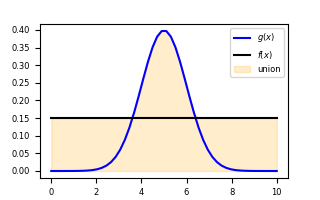
(a)

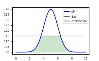
(b)

Figure 1: Illustration of the generalization of the union and intersection operations for (non-negative) functions: Union (a) and intersection (b) of $f(x)=0.15$ with $g(x)=\frac{1}{\sqrt{2\pi}}e^{-\frac{1}{2}(x-5)^{2}}$ in the interval $[0,10]$.

As illustrated in that figure, the multiset union corresponds to the union of the areas of the two functions, being therefore implemented by the maximum operation at each of the values of $x$. The multiset intersection of the areas corresponds to the minimum between the functions.

2.2 Jaccard Similarity

Let $\boldsymbol{x}$ and $\boldsymbol{y}$ be two non-zero $N\times 1$ dimensional vectors of non-negative values. The Jaccard similarity index between these two vectors can be expressed as (e.g. [11, 12, 14]):

$$\mathcal{J}(\boldsymbol{x},\boldsymbol{y})=\frac{\sum_{i=1}^{N}\min\left\{x_{i},y_{i}\right\}}{\sum_{i=1}^{N}\max\left\{x_{i},y_{i}\right\}}.$$ (5)

with $0<\mathcal{J}(\boldsymbol{x},\boldsymbol{y})\leq 1$ and $\mathcal{J}(\boldsymbol{x},\boldsymbol{y})=\mathcal{J}(\boldsymbol{y},\boldsymbol{x})$.

In the expression above, the $\min$ and $\max$ correspond to the multiset (e.g. [10]) operations with non-negative multiplicity respective to the set union and intersection operations from classic set theory. In addition, observe that the Jaccard operator is not bilinear, which contributes to its more intricate properties as compared to, e.g., the scalar product (e.g. [15]).

We can define [7] the Jaccard similarity of a scalar value $x$ with the vector $\boldsymbol{x}$ as

$$\mathcal{J}(x,\boldsymbol{x})=\frac{\sum_{i=1}^{N}\min\left\{x,x_{i}\right\}}{\sum_{i=1}^{N}\max\left\{x,x_{i}\right\}}.$$ (6)

Observe that the order of the elements of $\boldsymbol{x}$ does not matter, so that the above definition holds also for a non-empty set $X$ of non-negative values.

Given a random variable $X$ with a discrete set of possible values $x_{i}$ for $i=1,2\ldots$, each $x_{i}$ with an associated probability $p_{X}(i)$, we can define the Jaccard similarity of a value $x$ with the random variable $X$ as

$$\mathcal{J}_{X}(x)=\frac{\sum_{i=1}^{\infty}\min\left\{x,x_{i}\right\}p_{X}(i)}{\sum_{i=1}^{\infty}\max\left\{x,x_{i}\right\}p_{X}(i)}.$$ (7)

Notice that this is equivalent to Eq. (6) if we consider the $x_{i}$ here as the unique values in the vector x used in Eq. (6) and the $p_{i}$ here as $n_{i}/N$, where $n_{i}$ is the multiplicity of the value $x_{i}$ in the vector.

If we have a continuous random variable $X$ with a given probability density function (PDF) $p_{X}(x)$ we can define the Jaccard similarity of $x$ with $X$ as

$$\mathcal{J}_{X}(x) =\frac{\int_{0}^{\infty}\min\{x,\xi\}p_{X}(\xi)\,d\xi}{\int_{0}^{\infty}\max\{x,\xi\}p_{X}(\xi)\,d\xi}.$$ (8)

Notice that this is a generalization of Eq. (7) if we use

$$p_{X}(x)=\sum_{i=1}^{\infty}p_{X}(i)\delta(x-x_{i}),$$

with $\delta(x)$ the Dirac delta.

2.3 Similarity Means

The concept of similarity mean has been recently suggested [7, 8] as follows. Given a set of $N$ values $S$, which may correspond to a set of observations of a given random variable $X$, as well as a specific type of similarity index (e.g. Jaccard), the respective similarity mean corresponds to the value of $x$ comprised in the support of $X$ that yields the maximum similarity index. Observe, however, that as defined the similarity mean does not necessarily have to correspond to one of the elements of the set $S$.

The main motivation underlying the concept of similarity mean consists in the idea of obtaining a value $x$ that is as close as possible to the whole set of elements in $S$. As such, this concept bears a direct relationship with the role of centrality underlying the more traditional mean. In addition, it is interesting that similarity means be non-dimensional.

Because there are several types of similarity indices (e.g. [16, 17, 18, 19, 12]), an equal number of similarity means can be obtained, each of these inheriting the properties of the similarity index from which they derive.

The present work focuses on the means defined from the Jaccard similarity index, which is presented in Section 2.

Among several alternative similarity index, the Jaccard approach represents a particularly intuitive and powerful manner to compare two non-empty sets. Basically, this index quantifies how much the two sets intersect one another, normalized by their respective union. Therefore, the maximum value of 1 is obtained whenever the two sets are identical, while the minimum value of 0 results when the two sets have no common elements (no intersection).

Interestingly, the Jaccard index can be extended to multisets, and then to virtually any mathematical structure, including vectors, functions, matrices, fields, graphs, etc. [11, 12, 13]. Thus, the Jaccard index provides an effective approach to be considered in several scientific and technological areas, including but not limited to signal and image processing, pattern recognition, and artificial intelligence.

The main motivation to consider the Jaccard index as the basis for defining a respective similarity mean derives from the important properties that this specific index has been found to present (e.g. [11, 12, 13]). These include the fact that it is intrinsically normalized, taking values in the interval $[0,1]$, being also non-dimensional, highly selective and sensitive, while being robust to moderate perturbations of the data to be compares, as well as to the presence of eventual outliers.

3 The Jaccard Mean is Contained in the Original Values

One of the most interesting properties of the Jaccard similarity means corresponds to the fact, as shown in the following, that it necessarily coincides with one of the original values. This property is especially important because it simplifies the calculation of the means (only the original values need to be checked for maximum similarity), and also because it does not require the support of the random variable to be extended in order to incorporate a new value.

As the indices (order) of the sample values are immaterial, to simplify our argument we assume that the $N$ sample values are sorted in non-decreasing order, such that $x_{j}\leq x_{j+1}$ for $1\leq j\leq N-1$. Now, consider the case $x<x_{1}$. The minima in the numerator of Eq. (6) are always $x$, while the maxima in the denominator are always $x_{i}$, and we have

$$\mathcal{J}(x,\boldsymbol{x})=\frac{Nx}{s_{N}}=\frac{x}{\mu}\leq\frac{x_{1}}{\mu}=\mathcal{J}(x_{1},\boldsymbol{x}),$$ (9)

where we used the notation $s_{k}=\sum_{i=1}^{k}x_{i}$ and $\mu=s_{N}/N.$ On the other hand, for the case $x>x_{N}$ the minima in numerator of Eq. (6) are always $x_{i}$ and the maxima in the denominator are always $x$, such that

$$\mathcal{J}(x,\boldsymbol{x})=\frac{s_{N}}{Nx}=\frac{\mu}{x}\leq\frac{\mu}{x_{N}}=\mathcal{J}(x_{N},\boldsymbol{x}).$$ (10)

With this we see that the maximum of the Jaccard similarity is contained within the interval defined by the sample values, and it remains to show that it is reached at one of them.

For $x_{1}<x<x_{N}$, there will be a $k$, $1\leq k<N$, for which $x_{k}\leq x<x_{k+1}$. The minima in the numerator are $x_{i}$ for any $i\leq k$ and $x$ for the remaining $N-k$ values; the maxima in the denominator are $x$ for $i\leq k$ and $x_{i}$ for the remaining elements, resulting in

$$\mathcal{J}(x,\boldsymbol{x})=\frac{s_{k}+(N-k)x}{kx+(s_{N}-s_{k})}.$$ (11)

It is easy to see that Eq. (11) is valid also for $x$ assuming both limit values $x_{k}$ and $x_{k+1}$. Therefore, the derivative

$$\frac{d}{dx}\mathcal{J}(x,\boldsymbol{x})=\frac{N(s_{n}-s_{k})-ks_{n}}{\left(kx+(s_{N}-s_{k})\right)^{2}}$$ (12)

is zero only if

$$N(s_{n}-s_{k})=ks_{n},$$ (13)

which is independent of $x$. The Jaccard similarity in the interval between two samples is then either growing, with maximum at $x_{k+1}$, decreasing with maximum at $x_{k}$ or constant. We this we see that the Jaccard similarity for values of $x_{k}<x<x_{k+1}$ cannot be larger than at the sample values. In the special case where the derivative is zero, we have a degeneracy and could choose either $x_{k}$, $x_{k+1}$, or any value in the interval as the mean.

As an example, consider the set of values:

$$S=\left\{3,4,15,16\right\}$$ (14)

We have from the above developments that the Jaccard similarity mean of this set, $\bar{x}$, necessarily belongs to $S$. The Jaccard similarities between each of the four candidate elements and the set of values can thus be calculated as follows:

$$J(3,S) =\frac{\min(3,3)+\min(3,4)+\min(3,15)+\min(3,16)}{\max(3,3)+\max(3,4)+\max(3,15)+\max(3,16)}$$

$$=\frac{(3)(4)}{3+4+15+16}=\frac{6}{19}$$

$$J(4,S) =\frac{\min(4,3)+\min(4,4)+\min(4,15)+\min(4,16)}{\max(4,3)+\max(4,4)+\max(4,15)+\max(4,16)}$$

$$=\frac{3+(3)(4)}{(2)(4)+15+16}=\frac{15}{39}$$

$$J(15,S) =\frac{\min(15,3)+\min(15,4)+\min(15,15)+\min(15,16)}{\max(15,3)+\max(15,4)+\max(15,15)+\max(15,16)}$$

$$=\frac{3+4+(2)(15)}{(3)(15)+16}=\frac{37}{61}$$

$$J(16,S) =\frac{\min(16,3)+\min(16,4)+\min(16,15)+\min(16,16)}{\max(16,3)+\max(16,4)+\max(16,15)+\max(16,16)}$$

$$=\frac{3+4+15+16}{(4)(16)}=\frac{19}{32}$$

Therefore, the Jaccard similarity mean of the set $S$ above corresponds to the value $\bar{x}=15$, as this yields the maximum Jaccard similarity value $37/61$ with the set $S$.

Though simple, this example indicates that, even if the sough Jaccard mean is known to be contained in the set $S$, a total of $N^{2}$ minimum and maximum operations will still be required for its calculation, implying $\mathcal{O}(N^{2})$.

The main reason why the Jaccard mean is more computationally expensive to calculate than the arithmetic mean (which is $\mathcal{O}(N)$) is that these similarity indices are intrinsically non-linear, while the traditional average is linear.

In the next section, an algorithm is developed which allows the Jaccard mean to be calculated in $\mathcal{O}(N\log N)$.

4 Computing the Jaccard Mean

The above results suggest an efficient algorithm for the computation of the Jaccard mean of a sample of values. First, notice that the sign of the derivative of the Jaccard similarity is given by the sign of

$$\varsigma(k)=N(s_{n}-s_{k})-ks_{n}$$ (15)

But in this expression, the first term starts as a large positive value and decreases monotonically to zero with $k$, while the second term increases monotonically from zero with $k$. The result is that the derivative starts positive and decreases monotonically to a negative value. It is possible, therefore, to compute the Jaccard mean by the following $\mathcal{O}(N\log N)$ procedure:

1. Sort the sample values in non-decreasing order. Call $x_{i}$ the $i$-th value in this order.

2. Compute $s_{i}=\sum_{j=1}^{i}x_{j}$ for $1\leq i\leq N$.

3. Starting at $i=1$, keep computing $\varsigma(i)$ for successive values of $i$ while this expression is positive.

4. When you find an $m$ for which $\varsigma(m)$ is either negative or zero, use $x_{m}$ as the Jaccard mean.

Notice that, in this definition, for the degenerate case where $\varsigma(m)=0$, we are using the smallest value $x_{m}$, where we could have used $x_{m+1}$ as well. This is done for compatibility with the definition for continuous random variables, to be presented below, as in this case $x_{m}$ is the sample value with zero derivative.

In addition to being conveniently calculated numerically by using the above approach, it is also possible to obtain analytical expressions for the Jaccard mean of several discrete and continuous probability distributions, which is presented in the followins sections.

5 Discrete Distributions

In this section, basic analytic results are derived concerning the Jaccard mean of generic discrete distributions.

In Eq. (7), assuming that $x_{i}<x_{i+1}$ and that $x_{k}\leq x<x_{k+1}$ for some $k$

$$\mathcal{J}_{X}(x)=\frac{\sum_{i=1}^{k}x_{i}p_{X}(i)+x\sum_{i=k+1}^{\infty}p_{X}(i)}{x\sum_{i=1}^{k}p_{X}(i)+\sum_{i=k+1}^{\infty}x_{i}p_{X}(i)}.$$ (16)

Using

$$P_{X}(k) =\sum_{i=1}^{k}p_{X}(i)$$ (17)

$$m_{X}(k) =\sum_{i=1}^{k}x_{i}p_{X}(i)$$ (18)

$$\mu_{X} =\sum_{i=1}^{\infty}x_{i}p_{X}(i)$$ (19)

it becomes

$$\mathcal{J}_{X}(x)=\frac{m_{X}(k)+x\left(1-P_{X}(k)\right)}{xP_{X}(k)+\mu_{X}-m_{X}(k)}.$$ (20)

The previous result can be generalized for the computation of the Jaccard mean, notably that the mean is one of the distribution values and that it is the smallest value $x_{k}$ for which

$$\varsigma_{X}(k)=\mu_{X}\left(1-P_{X}(k)\right)-m_{x}(k)$$ (21)

is non-positive.

6 Continuous Distributions

As addressed in the present section, continuous probability distributions can also often have their respective Jaccard mean expressed in analytical terms.

We start by rewriting Eq. (8) as

$$\mathcal{J}_{X}(x) =\frac{\int_{0}^{\infty}\min\{x,\xi\}p_{X}(\xi)\,d\xi}{\int_{0}^{\infty}\max\{x,\xi\}p_{X}(\xi)\,d\xi}$$

$$=\frac{\int_{0}^{x}\min\{x,\xi\}p_{X}(\xi)\,d\xi+\int_{x}^{\infty}\min\{x,\xi\}p_{X}(\xi)\,d\xi}{\int_{0}^{x}\max\{x,\xi\}p_{X}(\xi)\,d\xi+\int_{x}^{\infty}\max\{x,\xi\}p_{X}(\xi)\,d\xi}$$

$$=\frac{\int_{0}^{x}\xi p_{X}(\xi)\,d\xi+\int_{x}^{\infty}xp_{X}(\xi)\,d\xi}{\int_{0}^{x}xp_{X}(\xi)\,d\xi+\int_{x}^{\infty}\xi p_{X}(\xi)\,d\xi}.$$

Using the notation

$$P_{X}(x) =\int_{0}^{x}p_{X}(\xi)\,d\xi$$ (22)

$$m_{X}(x) =\int_{0}^{x}\xi p_{X}(\xi)\,d\xi$$ (23)

$$\mu_{X} =\int_{0}^{\infty}\xi p_{X}(\xi)\,d\xi$$ (24)

we write

$$\mathcal{J}_{X}(x)=\frac{\left(1-P_{X}(x)\right)x+m_{X}(x)}{P_{X}(x)x+\mu_{X}-m_{X}(x)}.$$ (25)

If the PDF is such that $p_{X}(x)=0$ for $0<x<a$, then we have

$$\mathcal{J}_{X}(x)=\frac{x}{\mu_{X}},\quad 0\leq x\leq a,$$ (26)

which means that before $x=a$, $J_{X}(x)$ grows linearly. This is similar to Eq. (9). On the other hand, if the PDF is such that $p_{X}(x)=0$ for $x>b$, then

$$\mathcal{J}_{X}(x)=\frac{\mu_{X}}{x},\quad x\geq b,$$ (27)

and $J_{X}(x)$ decays with $1/x$ after $x=b$. This is similar to Eq. (10).

Also, $J_{X}(a)=a/\mu_{X}$ and $J_{X}(b)=\mu_{X}/b$ are only equal if $\mu_{X}=\sqrt{ab}$, which is only possible if $a=b$. And because in general $\mu_{X}>\sqrt{ab}$, $J_{X}(a)<J_{X}(b)$, and the Jaccard similarity function if asymmetrical in $a<x<b$, even if $p_{X}(x)$ is symmetrical, as can be seen in the uniform distributions of Figure 2.

To find the Jaccard mean we compute the derivative of Eq. (25) and equate it to zero. The derivative is

$$\frac{d}{dx}J_{X}(x)=\frac{\left(1-P_{X}(x)\right)\mu_{X}-m_{X}(x)}{\left(P_{X}(x)x+\mu_{X}-m_{X}(x)\right)^{2}}.$$ (28)

Therefore, the value $x$ that solve the equation

$$\varsigma_{X}(x)=\left(1-P_{X}(x)\right)\mu_{X}-m_{X}(x)=0$$ (29)

is the Jaccard mean $\bar{x}$ of $X$. If $p_{X}(x)=0$ in a finite region and it happens that simultaneously $\varsigma_{X}(x)=0$, then all corresponding values of $x$ are solutions to Eq. (29) and we have a degenerate Jaccard mean.

Notice that $1-P_{X}(x)$ decreases (non necessarily monotonically) as $x$ grows, while $m_{X}(x)$ grows (non necessarily monotonically) with $x$. Also, $\left(1-P_{X}(x)\right)\mu_{X}$ is initially $\mu_{X}$ and drops to 0 at infinity, while $m_{X}(x)$ is initially zero and grow to $\mu_{X}$ at infinity. So, if $p_{X}(x)$ is continuous, the derivative will necessarily be zero somewhere. Furthermore, $1-P_{X}(x)$ and $m_{X}(x)$ are constant only in regions where $p_{X}(x)=0$. This implies that

1. if $\varsigma_{X}(x)>0$, then $\bar{x}>x$, and

2. if $\varsigma_{X}(x)<0$, then $\bar{x}<x$.

7 Some Examples

Having developed analytical results concerning the Jaccard mean of discrete and continuous distributions, it is now interesting to look at some respective examples. We consider here the following distributions: uniform, exponential, truncated normal and power law.

7.1 Uniform distribution

Consider a random variable U with a uniform distribution between $\mu-d$ and $\mu+d$, that is

$$p_{U}(x)=\begin{cases}\frac{1}{2d}&\mu-d<x<\mu+d,\\ 0&\mbox{otherwise},\end{cases}$$ (30)

In the region of interest, we have

$$P_{U}(x) =\frac{x-\mu+d}{2d}$$

$$m_{U}(x) =\frac{x^{2}-(\mu-d)^{2}}{4d}$$

$$\mu_{U} =\mu.$$

Substituting in Eq. (25) we get

$$J_{U}(x)=\frac{4d\mu-(x-\mu-d)^{2}}{4d\mu+(x-\mu+d)^{2}}.$$ (31)

Substituting in Eq. (29) we get

$$\mu\left(1-\frac{x-\mu+d}{2d}\right)-\frac{x^{2}-(\mu-d)^{2}}{4d}=0,$$

whose positive solution is

$$\bar{x}=\left(\sqrt{4+\frac{d^{2}}{\mu^{2}}}-1\right)\mu.$$ (32)

This is always larger than the first moment $\mu$, being equal only when $d/\mu\rightarrow 0$. As, to include only positive values, $d$ has to be at most $\mu$, the largest possible value of $\bar{x}/\mu$ is $\sqrt{5}-1$.

Figure 2 depicts the Jaccard similarity and means for the uniform distribution. It is noticeable the above mentioned lack asymmetry of the similarity, even for this symmetric distribution. We also see the linear growth of the similarity before $\mu-d$ and de $1/x$ decay after $\mu+d$. Of interest is also the growth of the Jaccard mean with respect to the arithmetic mean as the distribution gets wider.

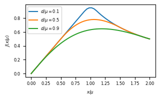
(a)

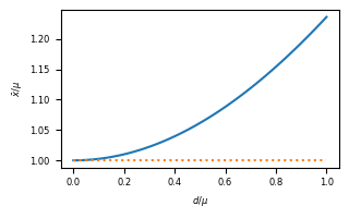
(b)

Figure 2: The Jaccard similarity and mean for the uniform distribution of Eq. (30). (a) The Jaccard similarity as a function of $x/\mu$, for some values of $d/\mu$. (b) The ratio $\bar{x}/\mu$ as a function of $d/\mu$; the dotted line shows the arithmetic average.

7.2 Exponential Distribution

Consider an exponential random variable $E$ with PDF

$$p_{E}(x)=\begin{cases}\lambda e^{-\lambda(x-x_{0})},&x>x_{0},\\ 0&x<x_{0}\end{cases}$$ (33)

We have

$$P_{E}(x) =1-e^{-\lambda(x-x_{0})}$$

$$m_{E}(x) =\frac{1}{\lambda}\left[1+\lambda x_{0}-(1+\lambda x)e^{-\lambda(x-x_{0})}\right]$$

$$\mu_{E} =\frac{1}{\lambda}+x_{0}.$$

Substituting in Eq. (25) we get

$$J_{E}(x)=\frac{1+\lambda x_{0}-e^{-\lambda(x-x_{0})}}{\lambda x+e^{-\lambda(x-x_{0})}}.$$ (34)

Substituting in Eq. (29) we get

$$e^{-\lambda(x-x_{0})}(2+\lambda x_{0}+\lambda x)=1+\lambda x_{0},$$

whose solution is

$$\bar{x}=-\left[2+\lambda x_{0}+W_{-1}\left(-(1+\lambda x_{0})e^{-2(1+\lambda x_{0})}\right)\right]\frac{1}{\lambda},$$ (35)

where $W_{-1}(x)$ is the -1 branch of the Lambert $W$ function.

Figure 3 shows the Jaccard similarity and means for the exponential distribution. Notice that the similarity decreases slowly for large $x$ and that for small $\lambda x_{0}$ the Jaccard mean is larger than the arithmetic mean, but this is soon reverted.

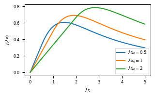
(a)

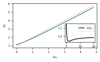
(b)

Figure 3: The Jaccard similarity and mean for the exponential distribution of Eq. (33). (a) The Jaccard similarity as a function of $\lambda x$ for some values of $\lambda x_{0}$. (b) The Jaccard mean $\bar{x}$, normalized by multiplying with $\lambda$, as a function of $\lambda x_{0}$; the dotted line show the arithmetic average; the inset shows the ratio of the Jaccard mean to the arithmetic mean as a function of $\lambda x_{0}$.

7.3 Truncated Normal

A normal distribution always has support in $x<0$. We work instead with a random variable $N$ distributed as a truncated normal

$$p_{N}(x)=\begin{cases}\frac{1}{\alpha}e^{-\frac{(x-\mu)^{2}}{2\sigma^{2}}}&x\geq 0,\\ 0&x<0,\end{cases}$$ (36)

where the normalization constant is

$$\alpha=\sigma\sqrt{\frac{\pi}{2}}\left(1+\operatorname{erf}\left(\frac{\mu}{\sqrt{2}\sigma}\right)\right),$$ (37)

where $\operatorname{erf}(x)$ is the error function. For this PDF we get:

$$P_{N}(x) =\frac{\operatorname{erf}\left(\frac{x-\mu}{\sqrt{2}\sigma}\right)+\operatorname{erf}\left(\frac{\mu}{\sqrt{2}\sigma}\right)}{1+\operatorname{erf}\left(\frac{\mu}{\sqrt{2}\sigma}\right)}$$

$$m_{N}(x) =\mu P_{N}(x)+\frac{\sigma^{2}}{\alpha}\left(e^{-\frac{\mu^{2}}{2\sigma^{2}}}-e^{-\frac{(x-\mu)^{2}}{2\sigma^{2}}}\right)$$

$$\mu_{N} =\mu+\frac{\sigma^{2}}{\alpha}e^{-\frac{\mu^{2}}{2\sigma^{2}}}.$$

These can be substituted in Eq. (25) (omitted here) and Eq. (29), giving

$$\sqrt{\frac{2}{\pi}}\frac{\alpha}{\sigma}e^{-\frac{(x-\mu)^{2}}{2\sigma^{2}}} -\left(2\frac{\mu\alpha}{\sigma^{2}}+e^{-\frac{\mu^{2}}{2\sigma^{2}}}\right)\operatorname{erf}\left(\frac{x-\mu}{\sqrt{2}\sigma}\right)$$

$$-\left(\sqrt{\frac{2}{\pi}}\frac{\alpha}{\sigma}-1\right)e^{-\frac{\mu^{2}}{2\sigma^{2}}}+\left(2-\sqrt{\frac{2}{\pi}}\frac{\alpha}{\sigma}\right)\frac{\mu\alpha}{\sigma^{2}}=0.$$ (38)

This equation can be solved numerically for given values of $\mu$ and $\sigma$.

Figure 4 shows the Jaccard similarity and mean for this distribution. Notice that, if $\mu$ is sufficiently larger than $\sigma$, such that the truncation of negative values does not significantly affect the distribution, there is a linear relationship from $\bar{x}/\sigma$ to $\mu/\sigma$, with a ratio close to one for large $\mu/\sigma$.

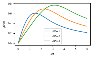
(a)

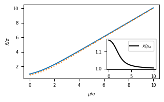
(b)

Figure 4: The Jaccard similarity and mean for the normal distribution of Eq. (36). (a) The Jaccard similarity as a function of $x/\sigma$, for some values of $\mu/\sigma$. (b) The Jaccard mean $\bar{x}$ normalized by $\sigma$, as a function of $\mu/\sigma$; the dotted line show the arithmetic average; the inset shows the ratio of the Jaccard mean to the arithmetic mean as a function of $\mu/\sigma$.

7.4 Power Law

Consider a random variable $P$ with the following distribution

$$p_{P}(x)=\begin{cases}\frac{\gamma-1}{x_{0}}\left(\frac{x}{x_{0}}\right)^{-\gamma}&x\geq x_{0},\\ 0&x<x_{0},\end{cases}$$ (39)

with $x_{0}>0$ and $\gamma>2$. For this PDF we get, in the region of interest ($x>x_{0}$):

$$P_{P}(x) =1-\left(\frac{x}{x_{0}}\right)^{-\gamma+1},$$

$$m_{P}(x) =\frac{\gamma-1}{\gamma-2}x_{0}\left[1-\left(\frac{x}{x_{0}}\right)^{-\gamma+2}\right]$$

$$\mu_{P} =.\frac{\gamma-1}{\gamma-2}x_{0}$$

These can be substituted in Eq. (25) giving

$$J_{P}(x)=\frac{(\gamma-1)(x/x_{0})^{\gamma-2}-1}{(\gamma-2)(x/x_{0})^{\gamma-1}+1}$$ (40)

and Eq. (29), giving

$$\left(\frac{x}{x_{0}}\right)^{-\gamma+2}+\left(\frac{x}{x_{0}}\right)^{-\gamma+1}=1.$$ (41)

This equation can be solved numerically for given values of $x_{0}$ and $\gamma$.

Figure 5 shows the Jaccard similarity and mean for this distribution. Larger values of $\gamma$, which imply a faster decay of the probability with $x$, have high similarity values more concentrated around the Jaccard mean, but smaller values os $\gamma$ show a very slow decay of the similarity with growing $x$. The Jaccard mean is in this case smaller than the arithmetic mean, specially for smaller values of $\gamma$.

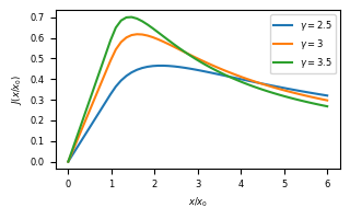
(a)

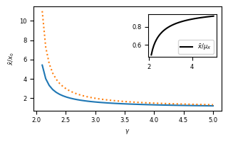
(b)

Figure 5: The Jaccard similarity and mean for the power law distribution of Eq. (39). (a) The Jaccard similarity as a function of $x/x_{0}$, for some values of $\gamma$. (b) The Jaccard mean $\bar{x}$ normalized by $x_{0}$ as a function of $\gamma$; the dotted line show the arithmetic average; the inset shows the ratio of the Jaccard mean to the arithmetic mean as a function of $\gamma$.

8 Relationship with the median

The Jaccard mean $\bar{x}$ is the solution to Eq. (29), and therefore

$$m(\bar{x})=\mu\left(1-P_{X}(\bar{x})\right).$$ (42)

If we substitute this in Eq. (25) we get

$$\mathcal{J}(\bar{x})=\frac{1-P_{X}(\bar{x})}{P_{X}(\bar{x})}.$$ (43)

But we know that $\mathcal{J}(x)\leq 1$, and therefore

$$P_{X}(\bar{x})\geq\frac{1}{2},$$ (44)

which means that the Jaccard mean is not smaller than the median.

9 Scaling and Translation

Let us now evaluate the effect of scaling and translation on the Jaccard mean. In addition to the intrinsic analytical interest of this analysis, it will also be shown that it is possible to control the bilateral symmetry of the Jaccard average by translating the original data elements.

9.1 Scaling

Given a random variable $X$ with Jaccard mean $\bar{x}$, if we create a scaled random variable $Y$ by making $y=ax$ with $a>0$, then we have

$$p_{Y}(y) =\frac{1}{a}p_{X}\left(\frac{y}{a}\right)$$

$$P_{Y}(y) =P_{X}\left(\frac{y}{a}\right)$$

$$m_{Y}(y) =am_{X}\left(\frac{y}{a}\right)$$

$$\mu_{Y} =a\mu_{X}.$$

and then the Jaccard mean of $Y$, $\bar{y}$ is the solution to

$$\mu_{Y}\left(1-P_{Y}(y)\right)-m_{Y}(y) =$$

$$a\left[\mu_{X}\left(1-P_{X}\left(\frac{y}{a}\right)\right)-m_{X}\left(\frac{y}{a}\right)\right] =0.$$

that is, $\bar{y}=a\bar{x}$.

It is also ease to see that, in this case

$$J_{Y}(y)=J_{X}(y/a).$$ (45)

9.2 Translation

If we construct a random variable $Y$ by shifting the values of a given random variable $X$ with Jaccard mean $\bar{x}$ by $c>0$, that is, $y=x+c$, then we get, for $y>c$,

$$p_{Y}(y) =p_{X}(y-c)$$

$$P_{Y}(y) =P_{X}(y-c)$$

$$m_{Y}(y) =m_{X}(y-c)+cP_{X}(y-c)$$

$$\mu_{Y} =\mu_{X}+c.$$

and the Jaccard mean $\bar{y}$ of $Y$ is the solution to

$$\mu_{Y}\left(1-P_{Y}(y)\right)-m_{Y}(y) =$$

$$\mu_{X}\left(1-P_{X}(y-c)\right)-m_{X}(y-c)+c\left(1-2P_{X}(y-c)\right) =0.$$

From this result we see that $\bar{y}=\bar{x}+c$ is only possible if $P_{X}(\bar{x})=1/2$, that is, if the Jaccard mean of the original distribution is equal to its median $h_{X}$. We also see that, as $c$ grows, when it gets much larger than $\mu_{X}$, the term $c\left(1-2P_{X}(y-c)\right)$ dominates the left hand side of the equation, that is, $\bar{y}\rightarrow h_{X}+c=h_{Y}$ as $c\rightarrow\infty$. Therefore, by shifting a distribution to the right we bring the Jaccard mean closer to the median.

This can be seen in Fig. 2(b), using the example of a uniform distribution: For this distribution, a translation corresponds to fixing $d$ and increasing $\mu$, which decreases the value of $d/\mu$, bringing $\bar{x}/\mu$ closer to one (see Eq. (32)). In Figure 6 we show the effect of a translation in our four example distributions. In all cases the Jaccard mean gets closer to the median as $c$ grows.

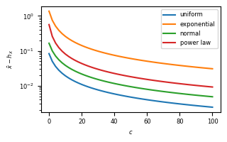
Figure 6: Effects of different translations on the Jaccard mean. We plot the difference between the Jaccard mean $\bar{x}$ and the median $h_{X}$ of the distribution, for different values do tranlation $c$ applied to the following initial distributions: a uniform distribution with $\mu=3$ and $d=1$; an exponential distribution with $\lambda=1/3$ and $x_{0}=0$; a truncated normal distribution with $\mu=3$ and $\sigma=1$; and a power law distribution with $\gamma=2.5$ and $x_{0}=1$. All initial distributions have $\mu_{X}=3$ (in the case of the truncated normal, approximately 3).

We also get

$$\mathcal{J}_{Y}(x+c)=\frac{\left(1-P_{X}(x)\right)x+m_{X}(x)+c}{P_{X}(x)x+\mu_{X}-m_{X}(x)+c},$$ (46)

that is, a value of $c$ is added in the numerator and denominator of the expression for $J_{X}(x)$, which increases the value of $\mathcal{J}_{Y}(y)$ with respect to the corresponding $\mathcal{J}_{X}(y-c)$. Now, consider a distribution for which most of the density is concentrated in an interval $[a,b]$. In this case, $\mathcal{J}_{X}(a)\approx a/\mu_{X}$ and $\mathcal{J}_{X}(b)\approx\mu_{X}/b$, but for $Y$ we have

$$\mathcal{J}_{Y}(a+c) \approx\frac{a+c}{\mu_{X}+c},$$ (47)

$$\mathcal{J}_{Y}(b+c) \approx\frac{\mu_{X}+c}{b+c},$$ (48)

which are closer to each other than $\mathcal{J}_{X}(a)$ and $\mathcal{J}_{X}(b)$.

In the special case where the original distribution $p_{X}(x)$ is symmetric, translation by a large $c$ results in: (i) getting the maximum of $\mathcal{J}_{Y}(y)$ (the Jaccard mean) closer to the center of the distribution $h_{X}+c$, and (ii) making the values at both sides of the center closer to each other. The result is a symmetrization of the profile of the generally asymmetric Jaccard similarity, at least in the region of high density $[a,b]$. This is shown in Fig. 7: for the symmetric uniform and Gaussian distributions, the asymmetry of the original Jaccard similarity (corresponding to the $c=0$ curve) is reduced for larger values of $c$. This could be useful in applications where symmetric similarity values are preferred.

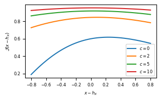
(a)

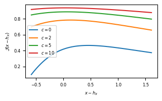
(b)

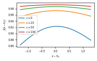
(c)

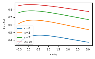
(d)

Figure 7: Effects of different translations on the Jaccard similarity. In each graph we plot the similarity in the region from the percentile 10% to the percentile 90% of the distribution. The plots are shifted such that the medians $h_{X}$ are at zero. The original distributions before translation are: (a) A uniform distribution with $\mu=1$ and $d=1$; (b) an exponential distribution with $\lambda=1$ and $x_{0}=0$; (c) a truncated normal distribution with $\mu=10$ and $\sigma=1$ (we use a larger $\mu$ here to avoid interference from the truncation, and we use proportionally larger values of $c$ to get the same $\mu_{X}/c$ rations); and a power law distribution with $\gamma=2.5$ and $x_{0}=1$.

10 Quantifying the Robustness of the Similarity Mean to Outliers

Suppose that data is being generated by a mixture of two random process, a “reference” process with PDF $p_{R}(x)$ and an “outlier” process with PDF $p_{O}(x)$, and that there is a probability $1-\eta$ of the data coming from the reference process and $\eta$ of coming from the outlier process, resulting in

$$p_{X}(x)=(1-\eta)p_{R}(x)+\eta p_{O}(x).$$ (49)

Figure 8 shows some examples of the effect of outliers on the Jaccard mean. For the examples shown, we see that, for small values of $\eta$, the Jaccard mean is less affected by outliers than the arithmetic mean: in Figures 8(a) and 8(c), where the outliers are larger than the reference values, the arithmetic mean grows faster with $\eta$ than the Jaccard mean, while in Figures 8(b) and 8(d), where the outliers are smaller than the reference values the arithmetic mean drops faster with $\eta$ than the Jaccard mean. Larger values of $d$ in Figures 8(a) and 8(b) or $\sigma$ in Figures 8(c) and 8(d), which imply broader distributions of values, increase the effect of outliers on the Jaccard mean. Furthermore, in Figures 8(a) and 8(c) we see a sharp transition of the value of the Jaccard mean to the region of the outliers, occurring for $\eta$ significantly less than $1/2$. This does not happen for $\eta<1/2$ in Figures 8(b) and 8(d), where the outliers are smaller than the reference values.

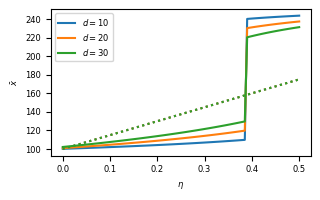
(a)

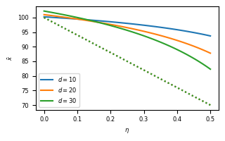
(b)

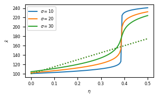
(c)

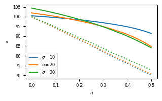
(d)

Figure 8: Effect of outliers as a function of the outlier density $\eta$. In (a) and (b) both reference and outlier distributions are uniform, following Eq. (30). In (c) and (d) both are truncated normal, following Eq. (36). The reference distributions always have $\mu=100$. The outlier distributions in (a) and (c) have $\mu=250$, and in (b) and (d) $\mu=40$. The other parameters are shown in the labels of the curves. Solid lines are the Jaccard mean, dotted lines of the same color are the arithmetic means.

To try to shed some light on these results, we will use the following simplifying assumptions:

1. $\eta\approx 0$, that is, outliers are rare;

2. there is a clear separation between the reference and outlier distributions, that is, there is a value $s$ for which:

   • if the outliers are larger than the reference values, $p_{R}(x)\approx 0$ for $x>s$ and $p_{O}(x)\approx 0$ for $x<s$; or

   • if the outliers are smaller than the reference values, $p_{R}(x)\approx 0$ for $x<s$ and $p_{O}(x)\approx 0$ for $x>s$.

With these assumptions, we evaluate the effect of the outliers on the Jaccard mean, that is, on the root of Eq. (29).

Large outliers

If the outliers are larger than the reference values, we have

$$P_{X}(x) \approx(1-\eta)P_{R}(x),$$

$$m_{X}(x) \approx(1-\eta)m_{R}(x),$$

$$\mu_{X} =(1-\eta)\mu_{R}+\eta\mu_{O}=\mu_{R}+\eta(\mu_{O}-\mu_{R}).$$

Substitution in Eq. (29) we get

$$\varsigma_{X}(x)=(\mu_{R}+\eta(\mu_{O}-\mu_{R}))\left[1-(1-\eta)P_{R}(x)\right]-(1-\eta)m_{R}(x),$$ (50)

and therefore, under our assumptions, the outlier distribution only affects the Jaccard mean through the outlier probability $\eta$ and the outlier mean $\mu_{O}$. Rearranging and keeping only linear terms in $\eta$ we get

$$\varsigma_{X}(x)=(1-\eta)\varsigma_{R}(x)+\eta\left[\mu_{O}(1-P_{R}(x))+\mu_{R}P_{R}(x)\right],$$ (51)

where $\varsigma_{R}(x)=\mu_{R}(1-P_{R}(x))-m_{R}(x)$. This expression tells us that

$$\varsigma_{X}(\bar{x}_{R})=\eta\left[\mu_{O}(1-P_{R}(\bar{x}_{R}))+\mu_{R}P_{R}(\bar{x}_{R})\right]$$

and that it has at this point inclination

$$\varsigma_{X}^{\prime}(\bar{x}_{R})=(1-\eta)\varsigma_{R}^{\prime}(\bar{x}_{R})=-(1-\eta)(\bar{x}_{R}+\mu_{R})p_{R}(\bar{x}_{R}),$$

from which we get the approximation (again, keeping only first order in $\eta$)

$$\bar{x}=\bar{x}_{R}+\eta\frac{\mu_{O}(1-P_{R}(\bar{x}_{R}))+\mu_{R}P_{R}(\bar{x}_{R})}{(\bar{x}_{R}+\mu_{R})p_{R}(\bar{x}_{R})}.$$ (52)

Small outliers

For the case of outliers smaller than the reference values, we have instead

$$P_{X}(x) \approx\eta+(1-\eta)P_{R}(x),$$

$$m_{X}(x) \approx\eta\mu_{O}+(1-\eta)m_{R}(x),$$

$$\mu_{X} =(1-\eta)\mu_{R}+\eta\mu_{O}=\mu_{R}-\eta(\mu_{R}-\mu_{O}).$$

Substitution in Eq. (29) we get

$$\varsigma_{X}(x)=(1-\eta)(\mu_{R}-\eta(\mu_{R}-\mu_{O}))\left[1-P_{R}(x)\right]-\eta\mu_{O}-(1-\eta)m_{R}(x).$$ (53)

Rearranging and keeping only linear terms in $\eta$ we get

$$\varsigma_{X}(x)=(1-\eta)\varsigma_{R}(x)-\eta\left[\mu_{O}P_{R}(x)+\mu_{R}(1-P_{R}(x))\right],$$ (54)

Again we have an inclination of

$$\varsigma_{X}^{\prime}(\bar{x}_{R})=-(1-\eta)(\bar{x}_{R}+\mu_{R})p_{R}(\bar{x}_{R}),$$

but now we have

$$\varsigma_{X}(\bar{x}_{R})=-\eta\left[\mu_{O}P_{R}(\bar{x}_{R})+\mu_{R}(1-P_{R}(\bar{x}_{R}))\right]$$

from which we get

$$\bar{x}=\bar{x}_{R}-\eta\frac{\mu_{O}P_{R}(\bar{x}_{R})+\mu_{R}(1-P_{R}(\bar{x}_{R}))}{(\bar{x}_{R}+\mu_{R})p_{R}(\bar{x}_{R})}.$$ (55)

Expressions (52) and (55) show that the response to outliers is inversely proportional to the density at the Jaccard mean of the undisturbed distribution. This explains why broader distributions are more sensitive to outliers, as seen in Figure 8, because broader distributions reduce the values of the density.

It is easy also to use these expressions, given a reference distribution and the average and the fraction of outliers to determine if the Jaccard mean is more or less sensitive to the outliers than the arithmetic average.

With regard to the sharp jump in the value of $\bar{x}$ with $\eta$ seen in Figure 8, we cannot use these expressions, as it occurs for a relatively large value of $\eta$. But the reason for the jump is easily seen, as the value of $\varsigma_{X}(x)$ depends on $P_{X}(x)$ and $m_{X}(x)$, and both of these vary very slowly if $p_{X}(x)\approx 0$. Therefore, in the separation region between $p_{R}(x)$ and $p_{O}(x)$, where both have small (or zero) densities, a large variation in $x$ is needed to effect a significant variation in $\varsigma_{X}(x)$. Thus, as soon as the value of the Jaccard mean is pulled by the outliers outside the high $p_{R}(x)$ region, the mean will be pulled fast all the way up to the region of large $p_{O}(x)$. The transition is faster the smaller the value of $p_{X}(x)$ in the separation region, and we see a discontinuity (as in Figure. 8(a)) if the density is zero in this region.

10.1 Outliers and Translation

Looking at Figure 8 and considering the discussion above it is clear that, even if the Jaccard mean is in general less sensitive to outliers than the arithmetic mean, the Jaccard mean can be pulled to the outlier region even before $\eta=0.5$ even if the outliers are larger and sufficiently frequent. This is not ideal in case there could be a high density of outliers in our sample. But, as seen in Section 9.2, a positive translation of the values pulls the Jaccard mean in the direction of the median. We can use this to prevent against a too early pull of the Jaccard mean to the outlier region: Before the analysis, the values are translated by a sufficiently large amount, which will pull the Jaccard mean in the direction of the median, which is, for $\eta<0.5$ necessarily in the region of the reference values.

This is illustrated in Figure 9. In this figure, we use the same reference and outlier distributions as in Figure 8(c) and Figure 8(d), but before computing the means we translate the distributions by a variable amount $c$. Afterwards, to facilitate the comparison, we subtract $c$ from the computed means. Our case of interest is depicted in Figure 9(a), where the outliers have large values. We see that for this case a value of $c$ around five times the arithmetic mean is able to reduce the value of the (translated) Jaccard mean, pulling it back to the region of the reference distribution, even for high $\eta$. Although Figure 9(b) shows that the translation does not help when the outliers have small values, it also shows that even then the (translated) Jaccard mean is less affected by outliers than the arithmetic mean. This shows that translation can be safely used even if there is a possibility of small value outliers.

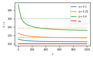
(a)

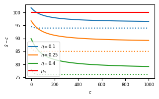
(b)

Figure 9: Effect of translation in the sensitivity to outliers of the Jaccard mean. We use a mixture distribution where reference and outlier distributions are truncated normal. The reference distribution has $\mu=100$ and the outlier distribution has $\mu=250$ in (a) and $\mu=40$ in (b). All distributions have $\sigma=30$. The original distributions are translated by $c$, the Jaccard and arithmetic means are calculated and we subtract $c$ from the results to facilitate the comparison. The red lines show the value of the arithmetic mean of the reference distribution.

11 Identifying Skewness in Datasets

The fact that the similarity means presents greater robustness to skewed outliers paves the way to a methodology for identification of possible bias in a data set, and for obtaining a more stable quantification of respective centrality previously suggested in [7].

The basic principle is that a dataset in presence of skewed perturbations will have its arithmetic mean to be noticeably distinct from some similarity means, such as Jaccard’s. The congruence between these two means $\mu_{a}$ and $\mu_{s}$ can be quantified, for instance, in terms of the following ratio:

$$\kappa=\frac{\mu_{a}-\mu_{s}}{|\mu_{s}|+1}$$ (56)

where the ‘+1’ in the denominator accounts for the eventual case $\mu_{s}=0$.

The methodology then consists of, given a dataset, calculating its respective arithmetic and similarity means and obtaining the respective coefficient $\kappa$ by using the above equation. The case in which $\kappa$ is large can then be taken as an indication of possible skewed perturbations (e.g. outliers) in the original dataset. In addition, in these cases the similarity mean provides a more stable indication of the data centrality. An application of this approach to the study of real-world sunsposts is described in the following section.

12 Application Example: Sunspots

The study of the number of sunspots along time has attracted continued interest from the scientific community (e.g. [20, 21, 22, 23]), not only for its intrinsic interest, but also for its possible effects on Earth. In particular, sunspots provide indications about possible subsequent solar flares, which can imply severe interference on radio communication and temporarily expand our atmosphere.

Thanks to long term continuing observations, the number of sunspots along time has been found to be nearly periodic, with a period of approximately 11 years defining the respective solar cycle (also known as Schwabe cycle). Figure 10 illustrates the sequence of sunspots observed in a monthly basis from 1750 to the present date [24], smoothed by using moving average with a window with total length of 19 months.

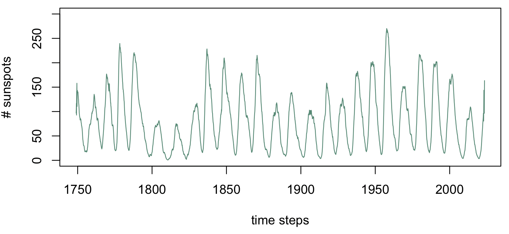
Figure 10: Smoothed (moving average with window with length of 19 months) representation of the monthly sequence of the number of sunspots as observed from 1750 to the present (Source: WDC-SILSO, Royal Observatory of Belgium, Brussels [24]).

It can be readily observed from Figure 10 that the numbers of sunspots change considerably along subsequent cycles. Figure 11 presents the superimposition of the 24 solar cycles initiating at 1755 up to 2008, which considered the cycles delimitation [25] followed by respective linear interpolation into 100 time steps.

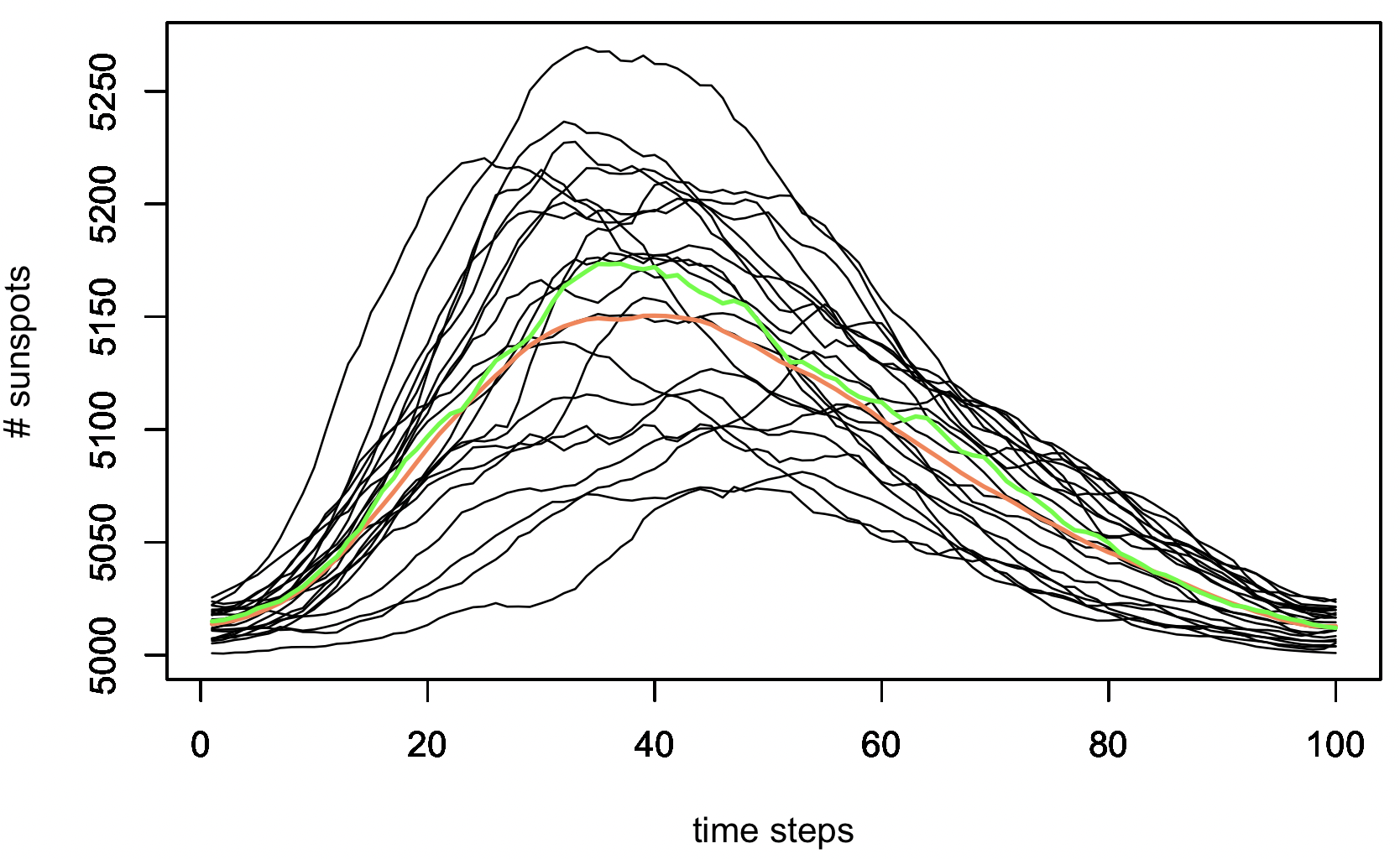
Figure 11: Superimposition of the number of sunspot along each solar cycle from 1755 to 2008. The duration of each original solar cycle was linearly interpolated into 100 time steps. The arithmetic and Jaccard means are shown in orange and green, respectively. Observe that the number of sunsposts in each solar cycle has been added to a constant offset value of 5000 as a means to enhance the symmetry of the Jaccard similarity (see Section 9.2)

The sunspots along each of the solar cycles shown in Figure 11 indicate that each cycle initiates with a minimum intensity, progresses to a respective maximum, then returning to minimum activity. The heights of the peaks can be found to present substantial dispersion that may be a consequence of data skewedness.

In order to obtain further indication about the skewedness of the solar cycles in Figure 11, we apply the methodology described in Section 11 considering the arithmetic and Jaccard means taken at each of the 100 interpolated time steps, which are shown as the orange and green curves, respectively.

The fact that the curve corresponding to the arithmetic mean resulted lower than the curve obtained for the Jaccard mean suggests a moderate skewedness of the solar cycles data. This relative displacement between the arithmetic and Jaccard means can be more objectively quantified in terms of the $\kappa$ index in Eq. 56. Figure 12 illustrates the values of this index in terms of the 100 time steps.

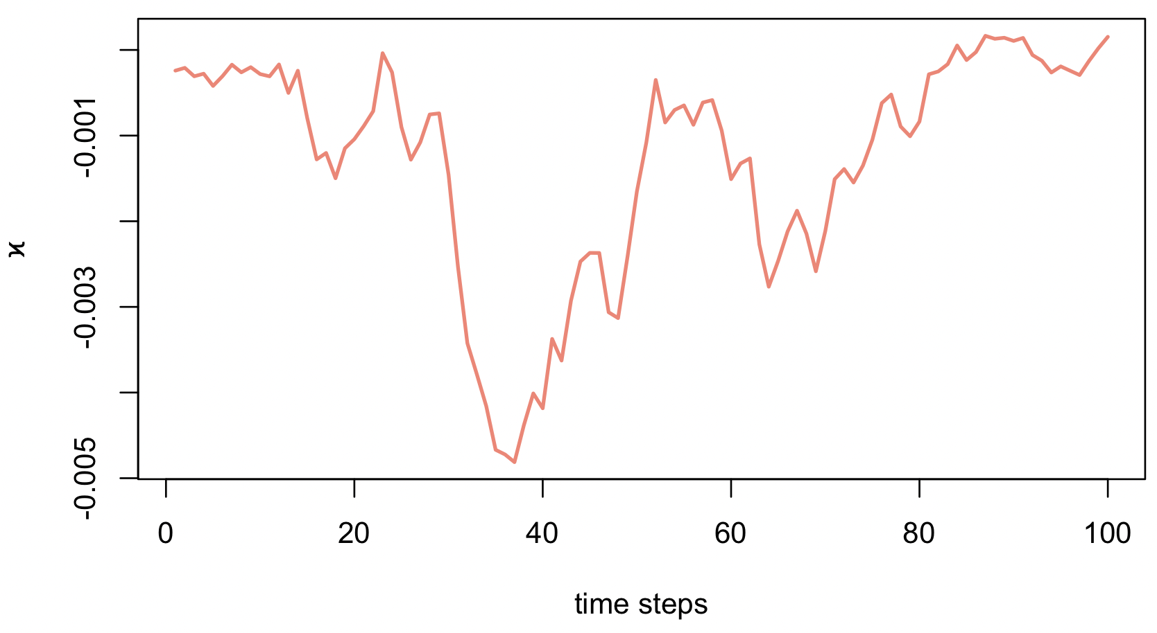
Figure 12: The $\kappa$ index between the arithmetic and Jaccard means obtained for the sunspots dataset. Most of the values are negative, indicating that the arithmetic mean tended to be smaller than the Jaccard counterpart. A peak of magnitude of $\kappa$ can be observed near time step 40, corresponding to the region most affected by the data skewness.

The obtained curves of arithmetic and Jaccard means, jointly with the respective $\kappa$ index, suggest the presence of an outlier group of solar cycles with smaller overall numbers of sunspots. Indeed, a closer inspection of the number of sunspots along each solar cycle confirms that the lower intensity cycles can be indeed understood as an outlier (or skewed) subgroup that ended up generating a multimodal distribution, thus biasing the arithmetic mean away from the respective Jaccard mean. No similar subgroups can be found with particularly large numbers of sunspots, which would have otherwise implied an opposite skewedness.

Because the Jaccard mean of a dataset has been shown in this work to necessarily correspond to one of the original data elements, it becomes possible to obtain a table indicating the solar cycle providing the number of sunspots taken as Jaccard means along each of the 100 time steps. This table is shown in Figure 13.

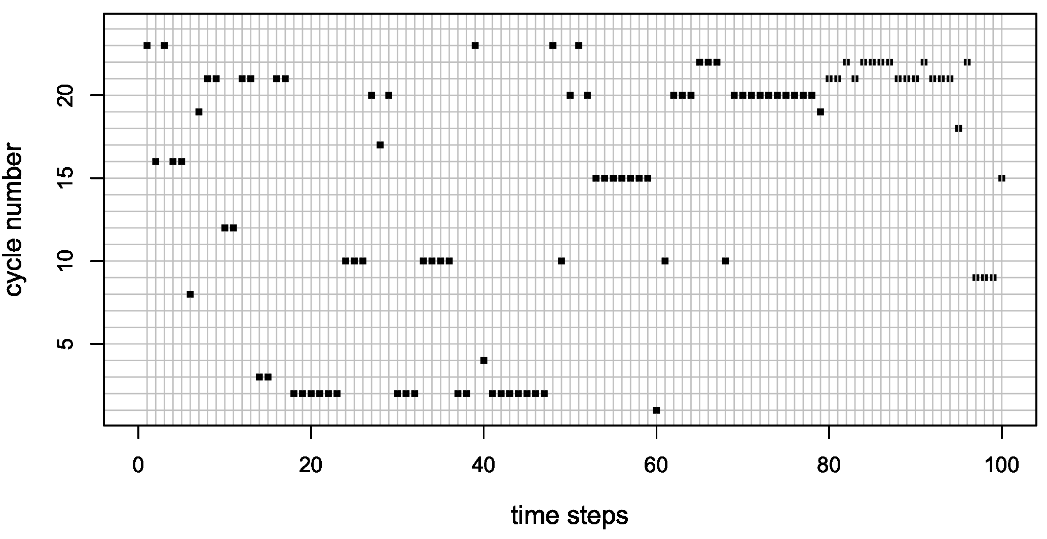
Figure 13: Identification of the solar cycle corresponding to the Jaccard mean obtained for each of the 100 time steps.

Interestingly, the number of sunspots in the solar cycles 2 (initiating on May 1766) and 10 (Dec. 1855) were chosen as Jaccard means for most of the the time steps between 18 and 47. Similarly, the number of sunspots from solar cycles 20 (Sep. 1964), 21 (Feb. 1976), and 22 (Aug. 1986) were taken as Jaccard mean for most of the time steps between 62 and 94.

In other words, the above results indicate that the solar cycles 2 and 10 can be understood as a prototype (or models) of the sunspots along the intermediate time steps, encompassing the region of the solar cycles where the skewness has been identified to be most intense. In an analogous manner, the solar cycles 20, 21, and 22 can be taken as prototypes of the trailing portion of the respective curves of numbers of sunspots.

Figure 14 depicts the histogram of occurrences of each solar cycle number taken as Jaccard means along the 100 time steps. The largest histogram counts are verified for solar cycles 2, 20, 21, 22 and 10.

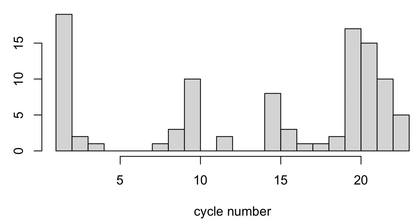
Figure 14: Histogram of occurrences of each solar cycle taken as Jaccard mean. Cycles 2, 10, 20, 21, and 22 are those appearing most frequently along the Jaccard means of the sunspot curves.

13 Concluding Remarks

The concept of mean plays a critical role not only in the physical sciences, but in almost every quantitative aspect of human activity. Its importance and ubiquity are implied by its ability to summarize a set of values in terms of single value, indicating the centrality of the values distribution.

While mean has been traditionally associated to arithmetic operations involving the original values to be summarized, the existence of several interesting similarity operators including the Jaccard and coincidence (e.g. [11, 12])) indices, motivates the definition and characterization of a respective similarity mean, which constituted the main objective of the present work.

After reviewing the basic concepts to be used, the concept of similarity means is described and discussed, with emphasis on the Jaccard similarity index, from which the Jaccard mean studied in the present work is derived.

Several studies and contributions are presented therefore, including the verification that the Jaccard mean of a discrete set of values necessarily corresponds to one of those values, the presentation of an effective algorithm for calculating the Jaccard mean, the analytic determination of the Jaccard mean respectively to several distributions (uniform, exponential, truncated normal, and power law), as well as a study of how the Jaccard mean is influenced by scaling and translation of the original data. The important issue of robustness to outliers was addressed next, including how it is influenced by translations of the original values.

The potential of the Jaccard mean for data analysis was then illustrated respectively to the study of sunspots cycles. More specifically, solar cycles were normalized along their domain, and their arithmetic and Jaccard means were estimated for each point along their domain. The fact that these two means resulted different allowed the identification of a group of outlier solar cycles, characterizede by smaller amplitudes.

The several reported contributions on concepts and methods related to the Jaccard mean pave the way to a wide range of possible subsequent related investigations. For instance, the reported results could be extended to data with negative values, and it would be also interesting to characterize and compare similarity means derived from other indices including Sørensen-Dice(e.g. [26]), overlap (e.g. [27]) and coincidence. Another particularly interesting development would be to extend the obtained results to higher dimensional spaces.

References

- [1] D. P. Bertsekas and J. N. Tsitsiklis. Introduction to Probability. Athena Scientific, 2008.
- [2] E. Kreyszig. Advanced Engineering Mathematics. Wiley and Sons, 2015.
- [3] M. H. DeGroot and M. J. Schervish. Probability and Statistics. Pearson, 2011.
- [4] H. Goldstein, C. Poole, and J. Safko. Classical mechanics, 2002.
- [5] L. da F. Costa. Modeling: The human approach to science. https://www.researchgate.net/publication/333389500_Modeling_The_Human_Approach_to_Science_CDT-8, 2019.
- [6] P. S. Bullen. Handbook of means and their inequalities. Springer, 1987.
- [7] L. da F. Costa. Similarity means: Seeking for robustness to outliers. https://www.researchgate.net/publication/371852653_Similarity_Means_Seeking_for_Robustness_to_Outliers, June 2023.
- [8] L. da F. Costa. Toward robust data classification. https://www.researchgate.net/publication/371935806_Toward_Robust_Data_Classification, 2023.
- [9] W. H. Press, S. A. Teukolsky, W. T. Vetterling, and B. P. Flannery. Numerical Recipes in C. Cambridge, 1992.
- [10] L. da F. Costa. Multisets. https://www.researchgate.net/publication/355437006_Multisets, 2021. [Online; accessed 21-Aug-2021].
- [11] L. da F. Costa. Further generalizations of the Jaccard index. https://www.researchgate.net/publication/355381945_Further_Generalizations_of_the_Jaccard_Index, 2021.
- [12] L. da F. Costa. On similarity. Physica A, 599:127456, 2022.
- [13] L. da F. Costa. Multiset neurons. Physica A, 609:128318, 2023.
- [14] L. da F. Costa. Coincidence complex networks. https://iopscience.iop.org/article/10.1088/2632-072X/ac54c3, 2022. J. Phys.: Complexity, (3): 015012.
- [15] L. da F. Costa. The scalar product from a panoramic perspective. https://www.researchgate.net/publication/375117484_The_Scalar_Product_from_a_Panoramic_Perspective, 2023.
- [16] M. Brusco, J. D. Cradit, and D. Steinley. A comparison of 71 binary similarity coefficients: The effect of base rates. PLOS One, 16(4):e0247751, 2021.
- [17] S.-H. Cha. Comprehensive survey on distance/similarity measures between probability density functions. Intl. J. Math. Models and Meths. in Appl. Sci., 1(4):300–307, 2007.
- [18] H. Wolda. Similarity indices, sample size and diversity. Oecologia, 50:296–302, 1981.
- [19] L. Hamers, Y. Hemeryck, G. Herweyers, M. Janssen, H. Ketters, H. Rousseau, and A. Vanhoutte. Similarity measures in scientometric research: The Jaccard index versus Salton’s cosine formula. Information Processing and Management, 25(3):315–318, 1989.
- [20] R. J. Bray and R. E. Loughhead. Sunspots. Dover Publications, 1964.
- [21] S. K Solanki and N. A. Krivova. Analyzing solar cycles. Science, 334(6058):916–917, 2011.
- [22] D. H. Hathaway, R. M. Wilson, and E. J. Reichmann. The shape of the sunspot cycle. Solar Physics, 151:177–190, 1994.
- [23] F. Clette, L. Svalgaard, J. M. Vaquero, and E. W. Cliver. Revisiting the sunspot number: A 400-year perspective on the solar cycle. Space Science Reviews, 186:35–103, 2014.
- [24] SILSO World Data Center. The International Sunspot Number. International Sunspot Number Monthly Bulletin and online catalogue, 1749–2021. http://www.sidc.be/silso/.
- [25] Wikipedia. Solar cycle. https://en.wikipedia.org/wiki/Solar_cycle, 2023.
- [26] A. Carass, S. Roy, A. Gherman, J. C. Reinhold, A. Jesson, T. Arbel, O. Maier, H. Handels, M. Ghafoorian, B. Platel, and et al. Evaluating white matter lesion segmentations with refined Sørensen-Dice analysis. Scientific reports, 10(1):8242, 2020.
- [27] M. K. Vijaymeena and K. Kavitha. A survey on similarity measures in text mining. Machine Learning and Applications, 3(1):19–28, 2016.