Spectroscopy of a single-carrier bilayer graphene quantum dot from time-resolved charge detection

Abstract

We measured the spectrum of a single-carrier bilayer graphene quantum dot as a function of both parallel and perpendicular magnetic fields, using a time-resolved charge detection technique that gives access to individual tunnel events. Thanks to our unprecedented energy resolution of $4\text{\,}\mathrm{\SIUnitSymbolMicro}\mathrm{e}\mathrm{V}$, we could distinguish all four levels of the dot’s first orbital, in particular in the range of magnetic fields where the first and second excited states cross ($B_{\perp}\lesssim$100\text{\,}\mathrm{m}\mathrm{T}$$). We thereby experimentally establish, the hitherto extrapolated, single-charge carrier spectrum picture and provide a new upper bound for the inter-valley mixing, equal to our energy resolution.

Quantum dots are an essential building block of electrical quantum circuits due to their diverse and versatile nature, positioning them as a primary physical platform for hosting qubits. Currently, semiconductor qubits rely on charge or spin for encoding quantum information [1, 2]. The valley degree of freedom, which stems from the crystal lattice symmetry, stands as a possible alternative. In Bernal-stacked bilayer graphene (BLG), both spin and valley are robust quantum numbers. In view of the recently measured strong valley blockade [3] leading to long relaxation times of a valley excited state [4] in a BLG double quantum dot, the valley degree of freedom emerges as a promising platform for quantum computing applications. In a single BLG quantum dot populated with a single charge carrier, the spin–orbit interaction lifts the four-fold degeneracy and leads to two Kramers pairs that consist (by construction) of states with both opposite valley and spin [5, 6, 7]. Breaking time-reversal symmetry by means of a perpendicular magnetic field lifts the remaining two-fold degeneracies of each pair, establishing a single-carrier BLG quantum dot as an ideal platform for implementing the valley-counterpart of the emblematic Loss-DiVincenzo spin-qubit [8]. In spite of the fast and recent developments in understanding the BLG quantum dot single- and multiple-particle spectra [7, 9, 10], those spectra have not been measured at zero and low magnetic field $B_{\perp}\lesssim$100\text{\,}\mathrm{m}\mathrm{T}$$, in the range where the first excited state crossing occurs. In particular, the magnitude of the spin–orbit splitting $\Delta_{\mathrm{SO}}\approx 40-$80\text{\,}\mathrm{\SIUnitSymbolMicro}\mathrm{e}\mathrm{V}$$ was never directly measured but rather extrapolated from finite-field data [11, 5, 6]. In addition, the relatively small value of $\Delta_{\mathrm{SO}}$, together with the large valley-Landé factor $18<g_{\mathrm{v}}<90$ [12, 13, 14, 10], requires a fine energy resolution to resolve each excited state of the spectrum at low fields, making the spectrum challenging to measure. This work presents a direct measurement of the spin–orbit splitting in a BLG quantum dot, as well as the single charge carrier low-magnetic field spectrum. We hereby experimentally establish the—so far simply assumed—single-charge carrier spectrum picture at zero and low magnetic fields and determine a new upper bound on the inter-valley mixing energy scale, equivalent to our energy resolution of $4\text{\,}\mathrm{\SIUnitSymbolMicro}\mathrm{e}\mathrm{V}$, a five-fold improvement on the previously standing upper bound [5]. Moreover, the tunnel rates into and out of the quantum dot were tuned down to unprecedentedly low values of $12.2\text{\,}\mathrm{H}\mathrm{z}$ at $B=$0\text{\,}\mathrm{T}$$. We overcame the previous requirement of a finite perpendicular magnetic field to reach sub-kHz tunnel rates [15, 16, 4], likely thanks to a relatively large displacement field ($D/\epsilon_{0}\approx$0.9\text{\,}\mathrm{V}\mathrm{/}\mathrm{n}\mathrm{m}$$, where $\epsilon_{0}$ is the vacuum permittivity), which opens a bandgap larger than the disorder potential. Finally, the time-resolved charge detection scheme used here for the spectroscopy, in combination with our low effective electron temperature ($46\text{\,}\mathrm{m}\mathrm{K}$), opens the door to measuring the relaxation time of the different excited states of the first charge carrier spectrum via Elzerman-readout [17] even at low magnetic fields.

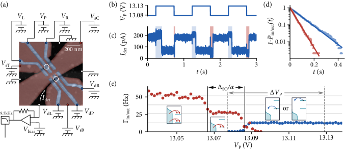
Figure 1: (a) False-colored atomic force microscopy image of the circuit and schematic of the measurement apparatus: a global backgate p-dopes the BLG where metallic top gates (in red) are patterned and polarized to form two conductive channels (dark areas). A second layer of top gates (in blue) enables the formation of a quantum dot in each channel, their location is indicated by white circles. The top left one is the system-dot, while the bottom right one is used as a detector. (b) The plunger gate voltage $V_{\mathrm{P}}(t)$ drive and (c) the simultaneously acquired detector current $I_{\mathrm{det}}(t)$ [marked in (a)]. The red (blue) shaded areas correspond to individual tunneling-in(-out) times. (d) Plot of the probability of a single hole to have already tunneled into (out) of the dot as a function of the waiting time, as red (blue) data points. The continuous lines represent the exponential probability expected from the average waiting times. (e) Average tunneling-in(-out) rates in red (blue) as a function of the plunger gate voltage $V_{\mathrm{P}}$. The two vertical black lines delimit the extent of the $\Gamma_{\mathrm{in}}=2\Gamma$ plateau. The two vertical dashed gray lines indicate the two values of $V_{\mathrm{P}}$ at which the data of (b–d) were acquired. The insets are schematics representing the different tunneling possibilities in and out of a dot with two levels that are each two-fold degenerate.

The rate at which a charge carrier tunnels into or out of a quantum dot is given by Fermi’s golden rule. This rate therefore depends on the spatial extent of the dot’s orbital wavefunction, the number of available micro-states, and selection rules. Notably, in the case of the transition from 0 to 1 carrier, there are no selection rules as the leads are neither valley- nor spin-polarized. The simplest model assumes that all of the micro-states of a given charge macro-state have an identical orbital wave function. In this case, the tunneling in (out) rate $\Gamma_{\mathrm{in(out)}}$ is expected to increase in steps proportional to the number of available micro-states [18, 19]:

$$\Gamma_{\mathrm{out}}(\varepsilon) =\Gamma\left[1-f(\varepsilon-\varepsilon_{\mathrm{g}})\right]$$ (1)

$$\Gamma_{\mathrm{in}}(\varepsilon) =\Gamma\left[f(\varepsilon-\varepsilon_{\mathrm{g}})+\sum_{i}f(\varepsilon-\varepsilon_{\mathrm{g}}-\Delta\varepsilon_{i})\right]$$ (2)

where $\Gamma$ is the tunnel rate intrinsic to the barrier configuration and the orbital’s spatial extent, $f$ is the Fermi-Dirac distribution, $\varepsilon_{\mathrm{g}}$ is the ground state energy, and $\Delta\varepsilon_{i}=\varepsilon_{i}-\varepsilon_{\mathrm{g}}$ is the energy difference between the excited state $i$ and the ground state.

It was previously shown that BLG quantum dots can be tuned such that a single orbital is populated at a time [20, 10]. Here, we take advantage of this tunability to determine the number of underlying spin and valley micro-states, by measuring the tunnel rates of the first charge carrier into and out of a single-carrier BLG quantum dot using a charge detector. Resolving the energy dependence of the rates then gives access to the spectrum and its magnetic field dependence.

The device is based on a stack of two-dimensional materials, which was assembled using the standard dry transfer technique [21, 22, 23]. It consists of a $35\text{\,}\mathrm{n}\mathrm{m}$ thick top hBN layer, the Bernal BLG sheet, a $28\text{\,}\mathrm{n}\mathrm{m}$ thick bottom hBN, and a graphite backgate layer. The BLG was subsequently contacted with 1D edge contacts [21]. Three metallic top gates ($3\text{\,}\mathrm{n}\mathrm{m}$ Cr, $20\text{\,}\mathrm{n}\mathrm{m}$ Au) were evaporated on top of the stack to define two conducting channels. Most notable is the central split gate (labeled sC in figure 1a), which has a nominal width of $140\text{\,}\mathrm{n}\mathrm{m}$ at the narrowest point. An additional set of top gates ($3\text{\,}\mathrm{n}\mathrm{m}$ Cr, $20\text{\,}\mathrm{n}\mathrm{m}$ Au) was also deposited, on top of a $26\text{\,}\mathrm{n}\mathrm{m}$ thick insulating layer of aluminum oxide deposited by atomic layer deposition. For this experiment, the backgate is polarized at $-7.25\text{\,}\mathrm{V}$ and the split gates (labeled sT, sC, and sB in figure 1a) at around $8.4\text{\,}\mathrm{V}$, yielding a displacement field of $0.9\text{\,}\mathrm{V}\mathrm{/}\mathrm{n}\mathrm{m}$ (assuming a relative dielectric constant of 3.5 for the hBN). At such displacement fields, the band-gap in BLG was previously measured to be $\sim$100\text{\,}\mathrm{m}\mathrm{e}\mathrm{V}$$ [24] (which, notably, is comparable to the gap achieved in InAs nanowires [25], where intrinsic tunnel rates as low as a few tens of hertz can be reached [26]). This arrangement of patterned gates enables us to form two capacitively coupled quantum dots, one of which acts as a charge detector for the other [27, 28, 29].

The tunnel rates were measured by driving the dot’s occupancy between the two charge states: 0 and 1 hole. The nearby charge detector enables us to acquire statistics on the random time taken by the charge carrier to tunnel into (out of) the dot. The bias across the detector-dot $V_{\mathrm{bias}}=$14\text{\,}\mathrm{\SIUnitSymbolMicro}\mathrm{V}$$ was kept small on purpose to avoid photo-assisted tunneling [30] and heating while the system-dot remained unbiased and its barriers were set to minimize the tunnel rates. A periodic square drive with amplitude $\Delta V_{\mathrm{P}}=$52\text{\,}\mathrm{m}\mathrm{V}$$ and frequency $1\text{\,}\mathrm{H}\mathrm{z}$, was applied to the system-dot’s plunger gate (labeled with $V_{P}$ in figure 1a), such that the dot’s most stable state alternated between single hole occupancy and empty. The detector current was channeled through an analog low-pass filter with a $9.5\text{\,}\mathrm{k}\mathrm{H}\mathrm{z}$ bandwidth to avoid any aliasing effect at our recording sampling frequency of $20\text{\,}\mathrm{k}\mathrm{H}\mathrm{z}$. The detector current was then digitally filtered with a notch filter centered at $698\text{\,}\mathrm{H}\mathrm{z}$ to reduce the triboelectric noise originating from vibrations of the dilution refrigerator’s pulse tube. In addition, a moving median filter spanning 15 points (corresponding to a $0.75\text{\,}\mathrm{m}\mathrm{s}$ time window) was utilized to enhance our signal-to-noise ratio, while keeping a sharp response of the detector current. An example of such a processed detector current trace is plotted in figure 1c, concurrently with the plunger gate drive in figure 1b. Figure 1c illustrates that the detector current jumps between two levels, centered around $60\text{\,}\mathrm{p}\mathrm{A}$ and $180\text{\,}\mathrm{p}\mathrm{A}$, corresponding to the first hole being out of and in the dot, respectively. By comparing the gate drive (figure 1b) and the detector’s response (figure 1c), it is clear that the tunnel events are not synchronized with the gate drive but rather occur with some delay. The delays for each individual event were measured and represented by the blue (red) shaded areas in figure 1c. For each configuration, we acquired 82 times $6\text{\,}\mathrm{s}$ long traces, adding up to $\sim$450 events, enabling us to obtain a reliable average waiting time for a charge carrier to tunnel into and out of the dot. It is possible to deduce the tunnel rates from the inverse of these average waiting times (see Supplementary Information for how we account for the finite time measurement window on the average rates). Importantly, as the sequential tunneling of a charge to or from a dot is a Poisson process, the distributions of waiting times are expected to be exponential. More specifically, the probability for the charge carrier to have tunneled in (out) after time $t$ should follow $P_{\mathrm{in(out)}}(t)=1-\exp{\Gamma_{\mathrm{in(out)}}t}$. Therefore, we collected the waiting times for each type of event, tunneling in and out. In figure 1d, we plot the quantity $1-n_{\mathrm{in(out)}}(t)/N_{\mathrm{in(out)}}$ which corresponds to $1-P_{\mathrm{in(out)}}(t)$, where $n_{\mathrm{in(out)}}(t)$ is the number of in (out) tunneling events that occurred after time $t$, and $N_{\mathrm{in(out)}}$ is the total number of tunneling in (out) events. The solid lines in figure 1d depict the exponential laws obtained from the inverse average waiting times, showing excellent agreement with the expected exponential decay of $1-P_{\mathrm{in(out)}}$.

We now turn to the dependence of the measured rates on the plunger gate voltage $V_{\mathrm{P}}$. We applied the previously described scheme for measuring the tunnel rates in addition to varying the plunger gate voltage, keeping the amplitude $\Delta V_{\mathrm{P}}$ of the square drive constant. The obtained average rates are plotted in figure 1e, where it can be seen that the tunneling out rate (in blue) is constant far away from the transition as expected from equation (1). This constitutes a calibration of the intrinsic tunnel rate $\Gamma=$12.9\text{\,}\mathrm{H}\mathrm{z}$$. By contrast, there is a step in $\Gamma_{\mathrm{in}}$, separating two plateaus at $2.12\Gamma=$27.4\text{\,}\mathrm{H}\mathrm{z}$$ and $4.02\Gamma=$51.7\text{\,}\mathrm{H}\mathrm{z}$$, respectively consistent with two and four accessible micro-states within the corresponding energy windows. The plateau $\Gamma_{\mathrm{in}}\approx 2\Gamma$ has an extent which corresponds to the spin–orbit splitting $\Delta_{\mathrm{SO}}$ at zero magnetic fields, which lifts the degeneracy between the two Kramers pairs [5, 6]. By multiplying the extent of this plateau by the independently characterized plunger gate lever arm $\alpha=0.003$, we obtain the value of the spin–orbit splitting $\Delta_{\mathrm{SO}}\approx 61\pm 4~{}\mu$eV. This value is compatible with previously reported values ranging between 40$~{}\mu$eV and 80$~{}\mu$eV [11, 5, 6]. However, all of these were extrapolated from high magnetic field data, while here we directly measured it at zero magnetic field. Our uncertainty results from thermal broadening (see supplementary information).

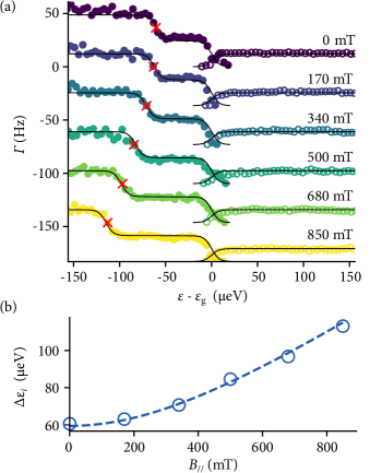
Figure 2: (a) Measured tunneling-in(-out) rates for different parallel magnetic fields. Each set of curves is plotted in a distinct color and with an incremental offset of $3\Gamma$ for clarity. The tunneling-in(-out) rates correspond to the full (open) symbols. (b) Parallel magnetic field dependence of the single-carrier spectrum. The data points are directly obtained from the red crosses of panel (a) where $\Delta\varepsilon_{2}=\Delta\varepsilon_{3}$, with uncertainty in energy given by the diameter of the circles. The dashed blue line is the result of a least-square optimization carried out on the data points, taking equation (4) as a model and with $\Delta_{\mathrm{SO}}$ as a unique fit parameter.

In the following, we focus on the magnetic field dependence of the excited state spectrum. The predicted energy separations between each of the three excited states and the ground state are given by [7]

$$\Delta\varepsilon_{1} =(g_{\mathrm{v}}+g_{\mathrm{s}})\mu_{\mathrm{B}}B_{\perp},$$ (3)

$$\Delta\varepsilon_{2} =\sqrt{[\Delta_{\mathrm{SO}}+g_{\mathrm{s}}\mu_{\mathrm{B}}B_{\perp}]^{2}+(g_{\mathrm{s}}\mu_{\mathrm{B}}B_{\parallel})^{2}},$$ (4)

$$\Delta\varepsilon_{3} =\sqrt{[\Delta_{\mathrm{SO}}+(g_{\mathrm{v}}-g_{\mathrm{s}})\mu_{\mathrm{B}}B_{\perp}]^{2}+(g_{\mathrm{s}}\mu_{\mathrm{B}}B_{\parallel})^{2}},$$ (5)

where $g_{\mathrm{v}}$ is the valley Landé factor, $g_{\mathrm{s}}=2$ the spin Landé factor, $\mu_{B}$ the Bohr magneton, and $B_{\perp(\parallel)}$ the magnitude of the perpendicular (parallel) magnetic field.

To further establish the obtained value of $\Delta_{\mathrm{SO}}$ at zero magnetic fields, we study the parallel magnetic field dependence of the excited state spectrum, keeping $B_{\perp}=0$. The full (open) circles in figure 2a are the measured $\Gamma_{\mathrm{in(out)}}$ for several values of parallel magnetic fields, where the extent of the plateau $\Gamma_{\mathrm{in}}=2\Gamma$ broadens as the magnetic field increases. The value of the intrinsic tunnel rate $\Gamma\approx$12.2\text{\,}\mathrm{H}\mathrm{z}$$ was first characterized by fitting each measured $\Gamma_{\mathrm{in(out)}}(\varepsilon)$ to equation (1), and averaging the obtained values for $\Gamma$. Then, the position of the ground state $\varepsilon_{\mathrm{g}}$ was established at each magnetic field (see Supplementary information for details on the ground state determination). We then identified the point $\Delta\varepsilon_{2}=\Delta\varepsilon_{3}$ where $\Gamma_{\mathrm{out}}=3\Gamma$ (see Supplementary information) for each magnetic field value and emphasized these points on figure 2a with red crosses. The energy differences $\Delta\varepsilon_{2}=\Delta\varepsilon_{3}$ are plotted as the blue circles in figure 2b. The dashed line is a fit to the expected splitting as given by equations 4 and 5, which simplify to $\Delta\epsilon_{2}=\Delta\epsilon_{3}=\sqrt{\Delta_{\mathrm{SO}}^{2}+(g_{s}\mu_{B}B_{\parallel})^{2}}$, in absence of a perpendicular magnetic field. Here, the only free parameter is $\Delta_{\mathrm{SO}}\approx$59\text{\,}\mathrm{\SIUnitSymbolMicro}\mathrm{e}\mathrm{V}$$, compatible with the value measured at zero magnetic field. As a confirmation of the previously determined values of $\Gamma$, $\varepsilon_{\mathrm{g}}$, and $\Delta_{\mathrm{SO}}$, we plot the black continuous lines in figure 2a that follow equations 1 and 2. The electronic temperature $T\approx$46\text{\,}\mathrm{m}\mathrm{K}$$ entering in the Fermi-Dirac distribution is separately determined from the average current values (see supplementary information). These black lines are not fits to the individual sets of points, but are directly the theoretical curves of equations 1 and 2, with all parameters independently determined.

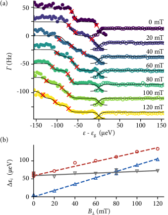
Figure 3: (a) Measured tunneling-in(-out) rates are plotted in full (open) symbols, for different magnetic field values each plotted in a distinct color and with an incremental offset of $2\Gamma$ for clarity. (b) Perpendicular magnetic field dependence of the single-carrier spectrum. The data points are directly obtained from the red crosses of panel (a). They are subsequently separated into three categories, each corresponding to an excited state: the blue upward triangles correspond to excited state 1, the gray downward triangles to excited state 2, and the red circles to excited state 3. The uncertainty in energy is given by the size of the symbols. The continuous gray line corresponds to equation (4), with $B_{\parallel}=$0\text{\,}\mathrm{T}$$, $\Delta_{\mathrm{SO}}=$59\text{\,}\mathrm{\SIUnitSymbolMicro}\mathrm{e}\mathrm{V}$$ and $g_{\mathrm{s}}=2$. The dashed blue and red lines correspond to the result of a least square optimization on $g_{\mathrm{v}}$ simultaneously performed on (3) and (5), to the data set with matching colors.

Finally, we look at the perpendicular magnetic field dependence of the spectrum, for which it is expected that all degeneracies are lifted. The tunneling rates $\Gamma_{\mathrm{in(out)}}$ were measured in steps of $20\text{\,}\mathrm{m}\mathrm{T}$ up to $120\text{\,}\mathrm{m}\mathrm{T}$, and are shown as full (open) circles in figure 3a. We used the same procedure as before to determine $\Delta\varepsilon_{i}$, by first characterizing $\varepsilon_{\mathrm{g}}$ and then identifying the points where $\Gamma_{\mathrm{in}}=\{1.5,2.5,3.5\}\Gamma$, indicated by the red crosses in figure 3a. The resulting values of $\Delta\varepsilon_{i}$ are plotted as a function of the perpendicular magnetic field in figure 3b. The points are then separated into three categories, differentiated by shapes and colors in figure 3b. Each set of points follows a linear dependence on $B_{\perp}$. The points located at the crossings are attributed to both possible sets. We subsequently plot the theoretical line for equation (4) that requires no fitting parameter, as a continuous gray line, using the previously determined $\Delta_{\mathrm{SO}}\approx$59\text{\,}\mathrm{\SIUnitSymbolMicro}\mathrm{e}\mathrm{V}$$, showing excellent agreement with the gray downward triangles. The two remaining sets correspond to the first and third excited states (equations 3 and 5), and require only one additional parameter $g_{\mathrm{v}}$, which is adjusted simultaneously for both sets. The red and blue dashed lines are the results of the parameter optimization for equations (3) and (5), giving $g_{\mathrm{v}}\approx 13.2$. Although on the low side of previously reported values, the valley Landé factor seems reasonable given the wide range of previously reported values from 18 to 90 [12, 13, 14, 10]. We then used this value of $g_{\mathrm{v}}$ as well as the previously determined parameters in equations 1 and 2 to plot the continuous black lines on figure 3a. The slight deviations occurring at higher energies could be due to an energy-dependence of the barrier, which in turn would be magnetic-field dependent, as observed in [19]. Noticeably, there is no valley mixing of the states up to our experimental resolution. This attests of the absence of crystalline defects in the bilayer graphene, over the spatial extent of the quantum dot’s wavefunction. We thus establish a new upper bound on the states valley-mixing of $4\text{\,}\mathrm{\SIUnitSymbolMicro}\mathrm{e}\mathrm{V}$ (limited by the electronic temperature in our device), five times lower than the previously reported value [5].

In summary, we measured the spectrum of a single-carrier bilayer graphene quantum dot with an energy resolution of $4\text{\,}\mathrm{\SIUnitSymbolMicro}\mathrm{e}\mathrm{V}$. We used a time-resolved charge detection technique that gives us direct access to the number of microstates in the system. This enabled us to resolve all four micro-states of a single-carrier quantum dot and their behavior as a function of both perpendicular and parallel magnetic fields. On the technological side, we demonstrated that the tunneling rates into and out of a bilayer graphene quantum dot could be made as low as $\sim$12\text{\,}\mathrm{H}\mathrm{z}$$ even in the absence of a magnetic field. Finally, our measurement scheme opens the door to measuring the lifetimes of the various excited states of different spin and/or valley nature in bilayer graphene quantum dots, close to zero magnetic fields. Interestingly, one has access here, in a small magnetic field range, to excited states that are either spin-, valley- or both spin and valley-polarized with respect to the ground state. Studying these would provide insights into the relative robustness of the spin and valley degree of freedom in bilayer graphene and the dominant mixing mechanism.

Appendix A Authors contributions

T.T., and K.W. grew the hBN. H.D. fabricated the device with inputs from M.M. and M.R.. A.O. and H.D. characterized and tuned the dots. S.C. and H.D. acquired and analyzed the data with inputs from T.I. and K.E.. H.D. wrote the manuscript with inputs from all authors.

Appendix B Acknowledgements

H.D. would like to thank Olivier Maillet, Everton Arrighi, Rebeca Ribeiro-Palau, and Artem Denisov for interesting discussions and suggestions. We acknowledge financial support by the European Graphene Flagship Core3 Project, H2020 European Research Council (ERC) Synergy Grant under Grant Agreement 951541, the European Innovation Council under grant agreement number 101046231/FantastiCOF, NCCR QSIT (Swiss National Science Foundation, grant number 51NF40-185902). K.W. and T.T. acknowledge support from the JSPS KAKENHI (Grant Numbers 21H05233 and 23H02052) and World Premier International Research Center Initiative (WPI), MEXT, Japan.

References

- Chatterjee et al. [2021] A. Chatterjee, P. Stevenson, S. De Franceschi, A. Morello, N. P. de Leon, and F. Kuemmeth, Semiconductor qubits in practice, Nature Reviews Physics 3, 157 (2021).
- Burkard et al. [2023] G. Burkard, T. D. Ladd, A. Pan, J. M. Nichol, and J. R. Petta, Semiconductor spin qubits, Reviews of Modern Physics 95, 025003 (2023).
- Tong et al. [2022] C. Tong, A. Kurzmann, R. Garreis, W. W. Huang, S. Jele, M. Eich, L. Ginzburg, C. Mittag, K. Watanabe, T. Taniguchi, K. Ensslin, and T. Ihn, Pauli Blockade of Tunable Two-Electron Spin and Valley States in Graphene Quantum Dots, Physical Review Letters 128, 067702 (2022).
- Garreis et al. [2023a] R. Garreis, C. Tong, J. Terle, M. J. Ruckriegel, J. D. Gerber, L. M. Gächter, K. Watanabe, T. Taniguchi, T. Ihn, K. Ensslin, and W. W. Huang, Long-lived valley states in bilayer graphene quantum dots (2023a), arxiv:2304.00980 [cond-mat, physics:quant-ph] .
- Banszerus et al. [2021] L. Banszerus, S. Möller, C. Steiner, E. Icking, S. Trellenkamp, F. Lentz, K. Watanabe, T. Taniguchi, C. Volk, and C. Stampfer, Spin-valley coupling in single-electron bilayer graphene quantum dots, Nature Communications 12, 5250 (2021).
- Kurzmann et al. [2021] A. Kurzmann, Y. Kleeorin, C. Tong, R. Garreis, A. Knothe, M. Eich, C. Mittag, C. Gold, F. K. de Vries, K. Watanabe, T. Taniguchi, V. Fal’ko, Y. Meir, T. Ihn, and K. Ensslin, Kondo effect and spin–orbit coupling in graphene quantum dots, Nature Communications 12, 6004 (2021).
- Knothe et al. [2022] A. Knothe, L. I. Glazman, and V. I. Fal’ko, Tunneling theory for a bilayer graphene quantum dot’s single- and two-electron states, New Journal of Physics 24, 043003 (2022).
- Loss and DiVincenzo [1998] D. Loss and D. P. DiVincenzo, Quantum computation with quantum dots, Physical Review A 57, 120 (1998).
- Tong et al. [2023] C. Tong, A. Kurzmann, R. Garreis, K. Watanabe, T. Taniguchi, T. Ihn, and K. Ensslin, Pauli blockade catalogue in bilayer graphene double quantum dots (2023), arxiv:2305.03479 [cond-mat] .
- Möller et al. [2023] S. Möller, L. Banszerus, A. Knothe, L. Valerius, K. Hecker, E. Icking, K. Watanabe, T. Taniguchi, C. Volk, and C. Stampfer, Understanding the fourfold shell-filling sequence in bilayer graphene quantum dots (2023), arxiv:2305.09284 [cond-mat] .
- Banszerus et al. [2020] L. Banszerus, B. Frohn, T. Fabian, S. Somanchi, A. Epping, M. Müller, D. Neumaier, K. Watanabe, T. Taniguchi, F. Libisch, B. Beschoten, F. Hassler, and C. Stampfer, Observation of the Spin-Orbit Gap in Bilayer Graphene by One-Dimensional Ballistic Transport, Physical Review Letters 124, 177701 (2020).
- Eich et al. [2018] M. Eich, F. Herman, R. Pisoni, H. Overweg, A. Kurzmann, Y. Lee, P. Rickhaus, K. Watanabe, T. Taniguchi, M. Sigrist, T. Ihn, and K. Ensslin, Spin and Valley States in Gate-Defined Bilayer Graphene Quantum Dots, Physical Review X 8, 031023 (2018).
- Kurzmann et al. [2019a] A. Kurzmann, M. Eich, H. Overweg, M. Mangold, F. Herman, P. Rickhaus, R. Pisoni, Y. Lee, R. Garreis, C. Tong, K. Watanabe, T. Taniguchi, K. Ensslin, and T. Ihn, Excited States in Bilayer Graphene Quantum Dots, Physical Review Letters 123, 026803 (2019a).
- Tong et al. [2021] C. Tong, R. Garreis, A. Knothe, M. Eich, A. Sacchi, K. Watanabe, T. Taniguchi, V. Fal’ko, T. Ihn, K. Ensslin, and A. Kurzmann, Tunable Valley Splitting and Bipolar Operation in Graphene Quantum Dots, Nano Letters 21, 1068 (2021).
- Gächter et al. [2022] L. M. Gächter, R. Garreis, J. D. Gerber, M. J. Ruckriegel, C. Tong, B. Kratochwil, F. K. de Vries, A. Kurzmann, K. Watanabe, T. Taniguchi, T. Ihn, K. Ensslin, and W. W. Huang, Single-Shot Spin Readout in Graphene Quantum Dots, PRX Quantum 3, 020343 (2022).
- Garreis et al. [2023b] R. Garreis, J. D. Gerber, V. Stará, C. Tong, C. Gold, M. Röösli, K. Watanabe, T. Taniguchi, K. Ensslin, T. Ihn, and A. Kurzmann, Counting statistics of single electron transport in bilayer graphene quantum dots, Physical Review Research 5, 013042 (2023b).
- Elzerman et al. [2004] J. M. Elzerman, R. Hanson, L. H. Willems van Beveren, B. Witkamp, L. M. K. Vandersypen, and L. P. Kouwenhoven, Single-shot read-out of an individual electron spin in a quantum dot, Nature 430, 431 (2004).
- Hofmann et al. [2016a] A. Hofmann, V. F. Maisi, C. Rössler, J. Basset, T. Krähenmann, P. Märki, T. Ihn, K. Ensslin, C. Reichl, and W. Wegscheider, Equilibrium free energy measurement of a confined electron driven out of equilibrium, Physical Review B 93, 035425 (2016a).
- Hofmann et al. [2016b] A. Hofmann, V. F. Maisi, C. Gold, T. Krähenmann, C. Rössler, J. Basset, P. Märki, C. Reichl, W. Wegscheider, K. Ensslin, and T. Ihn, Measuring the Degeneracy of Discrete Energy Levels Using a $\mathrm{GaAs}/\mathrm{AlGaAs}$ Quantum Dot, Physical Review Letters 117, 206803 (2016b).
- Garreis et al. [2021] R. Garreis, A. Knothe, C. Tong, M. Eich, C. Gold, K. Watanabe, T. Taniguchi, V. Fal’ko, T. Ihn, K. Ensslin, and A. Kurzmann, Shell Filling and Trigonal Warping in Graphene Quantum Dots, Physical Review Letters 126, 147703 (2021).
- Wang et al. [2013] L. Wang, I. Meric, P. Y. Huang, Q. Gao, Y. Gao, H. Tran, T. Taniguchi, K. Watanabe, L. M. Campos, D. A. Muller, J. Guo, P. Kim, J. Hone, K. L. Shepard, and C. R. Dean, One-Dimensional Electrical Contact to a Two-Dimensional Material, Science 342, 614 (2013).
- Yankowitz et al. [2019] M. Yankowitz, Q. Ma, P. Jarillo-Herrero, and B. J. LeRoy, Van der Waals heterostructures combining graphene and hexagonal boron nitride, Nature Reviews Physics 1, 112 (2019).
- Purdie et al. [2018] D. G. Purdie, N. M. Pugno, T. Taniguchi, K. Watanabe, A. C. Ferrari, and A. Lombardo, Cleaning interfaces in layered materials heterostructures, Nature Communications 9, 5387 (2018).
- Icking et al. [2022] E. Icking, L. Banszerus, F. Wörtche, F. Volmer, P. Schmidt, C. Steiner, S. Engels, J. Hesselmann, M. Goldsche, K. Watanabe, T. Taniguchi, C. Volk, B. Beschoten, and C. Stampfer, Transport Spectroscopy of Ultraclean Tunable Band Gaps in Bilayer Graphene, Advanced Electronic Materials 8, 2200510 (2022).
- Barker et al. [2019] D. Barker, S. Lehmann, L. Namazi, M. Nilsson, C. Thelander, K. A. Dick, and V. F. Maisi, Individually addressable double quantum dots formed with nanowire polytypes and identified by epitaxial markers, Applied Physics Letters 114, 183502 (2019).
- Barker et al. [2022] D. Barker, M. Scandi, S. Lehmann, C. Thelander, K. A. Dick, M. Perarnau-Llobet, and V. F. Maisi, Experimental Verification of the Work Fluctuation-Dissipation Relation for Information-to-Work Conversion, Physical Review Letters 128, 040602 (2022).
- Field et al. [1993] M. Field, C. G. Smith, M. Pepper, D. A. Ritchie, J. E. F. Frost, G. A. C. Jones, and D. G. Hasko, Measurements of Coulomb blockade with a noninvasive voltage probe, Physical Review Letters 70, 1311 (1993).
- Sprinzak et al. [2002] D. Sprinzak, Y. Ji, M. Heiblum, D. Mahalu, and H. Shtrikman, Charge Distribution in a Kondo-Correlated Quantum Dot, Physical Review Letters 88, 176805 (2002).
- Kurzmann et al. [2019b] A. Kurzmann, H. Overweg, M. Eich, A. Pally, P. Rickhaus, R. Pisoni, Y. Lee, K. Watanabe, T. Taniguchi, T. Ihn, and K. Ensslin, Charge Detection in Gate-Defined Bilayer Graphene Quantum Dots, Nano Letters 19, 5216 (2019b).
- Leturcq et al. [2008] R. Leturcq, S. Gustavsson, M. Studer, T. Ihn, K. Ensslin, D. C. Driscoll, and A. C. Gossard, Frequency-selective single-photon detection with a double quantum dot, Physica E: Low-dimensional Systems and Nanostructures 40, 1844 (2008).