A Cosheaf Theory of Reciprocal Figures: Planar and Higher Genus Graphic Statics

Abstract

This paper introduces cellular sheaf theory to graphical methods and reciprocal constructions in structural engineering. The elementary mechanics and statics of trusses are derived from the linear algebra of sheaves and cosheaves. Further, the homological algebra of these mathematical constructions cleanly and concisely describes the formation of 2D reciprocal diagrams and 3D polyhedral lifts. Additional relationships between geometric quantities of these dual diagrams are developed, including systems of impossible edge rotations. These constructions generalize to non-planar graphs. When a truss embedded in a torus or higher genus surface has a sufficient degree of axial self stress, we show non-trivial reciprocal figures and non-simply connected polyhedral lifts are guaranteed to exist.

1 Introduction

Graphic statics consists of a family of techniques for investigating the static equilibrium solutions of structures geometrically. As early as the 18th century, Varignon [1] introduced the concept of the funicular polygon and a polygon of forces to maintain structural equilibrium within a loaded structure [2]. Over a century later the foundational properties of reciprocal figures were further developed by Maxwell [3, 4], Cremona [5, 6], and Rankine [7], among others. These graphical methods were widely used by designers such as Antoni Gaudí, Heinx Isler and Frei Otto among others to find structurally efficient and beautiful structural forms [8].

In recent times graphical methods have experienced a renaissance of interest and attention, spurred on by, e.g., structural design [9, 10], optimization [11, 12], and education [13]. These methods have been utilized in Crapo and Whiteley’s study of rigidity theory [14, 15], Calladine and Pellegrino’s work on tensegrity structures [16, 17], and Tachi’s work on flexible origami structures [18]. The algebraic foundations of the theory have been further solidified by Micheletti [19], Van Mele and Block [20], and many others. McRobie, Konstantatou, and collaborators have further developed the understanding of kinematics and virtual work of reciprocal structures [21, 22].

Great strides have been made recently in the understanding and adoption of 3D graphic statics [2]. This theory has been proven valuable in the design and analysis of compressed concrete [23, 24] and glass structures [25]. With the additional challenges brought by the extra dimension, many researchers have advanced the mathematical understanding the construction of [26, 27, 28] and the mechanical properties of this spatial duality [29, 30].

1.1 Background

Although the most interesting current work is happening in 3D graphic statics, it is nevertheless true that any advances here must rest on a firm platform of 2D graphic statics. We therefore focus on a novel approach to 2D graphic statics as a stepping stone towards future foundational development in 3D.

In 2D graphic statics, a finite abstract graph $G$ is embedded in the plane with edges sent to straight lines, forming a mechanical truss with free-rotating joints known collectively as a form diagram. This truss may admit non-trivial axial self stresses—an assignment of an internal tension or compression force to each edge such that these forces mutually cancel over vertices. The combined free body diagram of axial forces is an embedding of the dual graph $\tilde{G}$ in the plane called a reciprocal figure or force diagram. The internal tension or compression force vectors on the primal graph form the edges of the dual, pictured in Figure 1. Through this process, the internal stresses can be visualized and understood graphically, revealing the rich underlying linear algebraic relationships.

In structural analysis, local quantities considered in static analysis, such as stresses over edges, coalesce into global properties of the truss such as axial self stress. This conglomeration of local data constrained by linear relationships is naturally described by the data structures known as cellular sheaves and cosheaves [31]. These are the discrete analogue of (continuous) sheaves, widely used in topology, algebraic geometry, logic, and other mathematical fields [32, 33]. Initially developed in the theses of Shepard [34] and Curry [35], cellular sheaves (and their cosheaf duals) have found applications in network coding [36], Reeb graphs [37], logic circuits [38], and pursuit and evasion games [39]. Exciting recent work has applied sheaves towards persistent homology [40, 41, 42], distributed optimization [43], graph neural networks [44, 45, 46], distributed consensus and flocking [47], opinion dynamics [47, 48, 49], and lattice theory [50, 51]. In this paper, we continue this program and extend previous work [52] applying cellular sheaf theory to the geometric structures encountered in graphic statics.

Many of these recent applications of cellular sheaves to applied problems were presaged by work decades earlier which did not have the simpler cellular theory available. Excellent examples include Schapira’s and Viro’s independent works on Euler calculus for sheaves of constructible functions with applications to image analysis [53, 54]. In similar fashion, Billera and Yuzvinsky independently developed cosheaves of piecewise polynomial splines, commonly used in architecture, design, and font systems [55, 56]. In graphic statics, sheaves were also explored as an approach decades ago. Beginning in the 1980s, Crapo [57, 58] used sheaves and homological methods to describe structural relations. Alongside Crapo, Whiteley developed a cosheaf theory not unlike that described here, then coined geometric homology [59]. Other matrix methods have been developed to algebraically formulate reciprocity without the full groundwork of sheaves and their cohomology [20, 60, 21]. Projective duality has been utilized in parts to develop reciprocal relations [61, 62, 63]. Our contributions via cellular sheaf theory unify and extend these threads with a theory that is both simpler and more powerful.

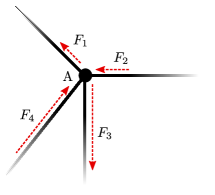
(a)

(b)

Figure 1: The crux of reciprocity. Tension or compression forces along bars are transferred to node A where they sum to zero (a). When placed tip to tail using a clockwise orientation, these force vectors form the boundary of a dual polygon A, pictured in (b).

1.2 Outline and Contributions

This paper is a self-contained introduction to a cosheaf theory of 2D graphic statics. This includes the statics of planar graphs, extended to a cellular structure on the 2-sphere $S^{2}$ by filling in faces within graph cycles. Adapting to more complex cellular topology beyond $S^{2}$ allows for the graphical analysis of non-planar graphs. There are several nuances to this extension which are discussed after the grounding planar theory is developed. These fundamental findings are expressed using the homological algebra of cellular sheaves and cosheaves developed in Section 2.

In Section 3, we introduce the constant cosheaf, force cosheaf, linkage sheaf, and position sheaf, which serve as the essential foundation for the foundation of sheaf-theoretic graphic statics. These constructions are purely in terms of vector spaces and linear maps, structured in a manner that respects the cellular topology. Additionally, we demonstrate that Maxwell’s counting rule for frames can be interpreted as an instance of the cellular cosheaf Euler characteristic, and the stiffness matrix is an instance of the sheaf (Hodge) Laplacian.

In Section 4.1 two dimensional planar graphic statics is developed, where Theorem 33 characterizes the homological relationship between a planar graph and its dual graph embedding. We describe reciprocity between the force cosheaf and position sheaf, revealing relations between a force diagram and its reciprocal form diagrams. These connections extend the work of previous authors on mechanical duality in planar graphic statics [60, 21].

Theorem (37,42).

Suppose $(X,p)$ and $(\tilde{X},q)$ are planar reciprocal diagrams over the plane $\mathbb{R}^{2}$. The following vector spaces are isomorphic:

• The space of mechanisms and global rotations of $(X,p)$.

• The space of parallel deformations of $(X,p)$ up to global translation.

• The space of impossible edge rotations over $(\tilde{X},q)$.

• The space of axial self stresses over $(\tilde{X},q)$.

• The space of pure self shear stresses over $(\tilde{X},q)$.

• The space of vertical polyhedral lifts of $(\tilde{X},q)$ up to shifts of a global affine function.

We note that here $X$ and $\tilde{X}$ must consist of nonsingular polygons, where each polygonal cell is a topological disk with boundary consisting of lower dimensional polygonal cells. This is a general condition on cells to disallow degenerate boundary maps. See also the full definition of a regular cell complex [35].

Section 4.3 explores an alternative approach where the cells are vertically lifted off of the plane to a polyhedron in 3D. This process of lifting a self-stressed graph is widely known as the Maxwell–Cremona correspondence. The homological relationships governing these lifts are formally expressed in Theorem 42 using the language of cosheaves.

Section 5 delves into the extensions of planar graphic statics to non-spherical topology. This section addresses the construction of force and form diagrams from non-planar graphs, allowing for a broader range of structural configurations. Assurances for the existence of dual diagrams are derived in terms of the genus of the cell structure. In essence, as long as the dimensions of equilibrium stresses exceeds a multiple of the one-dimensional holes present in the topology, the presence of dual diagrams is guaranteed. This insight highlights the role played by topological characteristics of the cell structure.

Theorem (43).

Suppose $(X,p)$ is a regular cellular decomposition of an oriented surface of genus $g$ realized in $\mathbb{R}^{2}$. If the dimension of self stress exceeds $4$ times the genus ($\dim H_{1}\mathcal{F}>4g$), then there exists a non-trivial parallel realization of $\tilde{X}$ in $\mathbb{R}^{2}$. The oriented length of each dual edge is equal to the force within its corresponding primal edge.

Theorem 43 presents a significant extension of 2D graphic statics to encompass non-planar graphs. A similar bound to Theorem 43 can be derived for polyhedral lifts. Here, graph edges and faces may overlap in the plane, lifting to a toroidal or higher genus polyhedra.

Theorem (45).

Suppose $(X,p)$ is a regular cellular decomposition of an oriented surface of genus $g$ realized in $\mathbb{R}^{2}$. If the dimension of self stress $\dim H_{1}\mathcal{F}$ is greater than $6g$, then there exists a non-trivial polyhedral lift to $\mathbb{R}^{3}$.

The existence of non-trivial reciprocal diagrams and polyhedral lifts has previously been linked to zero “face-edge cycles” by Crapo and Whiteley [15]. The two bounds above simplify and streamline the discovery process.

2 Sheaves, Cosheaves, and Structures

Cellular sheaves and cosheaves are discrete mathematical structures that assign algebraic data to the cells of a topological complex. These structures offer a versatile scaffolding for modeling a variety of abstract and physical phenomena. By assigning vector spaces to cells and defining linear maps between adjacent cells, these models allow for the representation of distributed vector-valued data. The pursuit of globally consistent data, where vectors assigned to cells adhere to all local linear constraints, leads to a general concept of global equilibrium.

For more comprehensive background on sheaves and cosheaves the theses of Curry [35] and Hansen [64] are excellent sources. These provide a deeper background and understanding of the concepts presented here.

2.1 Cellular Cosheaves

Cosheaves allocate individualized vector spaces to individual cells, allowing for a localized assignment of data.

Definition 1 (Cellular Cosheaf).

Given a finite regular cell complex $X$, a cellular cosheaf $\mathcal{K}=\mathcal{K}_{X}$ over $X$ consists of the assignment

• to each cell $c\in X$ a finite dimensional vector space $\mathcal{K}_{c}$ with inner product called the stalk of $\mathcal{K}$ at $c$ and,

• to incident cells $c\lhd d$ in $X$ a linear extension map $\mathcal{K}_{d\rhd c}:\mathcal{K}_{d}\to\mathcal{K}_{c}$.

Cosheaves, by nature, map data downward in cell dimension. Extension maps transfer data from face stalks to edge stalks, and subsequently from edge stalks to vertex stalks. By selecting appropriate bases for these stalks, extension maps can be explicitly represented as matrices. While definition 1 is extremely general, the data representation and behavior of a specific cosheaf can be programmed by choosing stalks and extension maps.

Definition 2 (Constant Cosheaf).

For $V$ a finite dimensional vector space, the constant cosheaf $\overline{V}$ over a cell complex $X$ is the cosheaf with stalks $\overline{V}_{c}=V$ over every cell $c$. Extension maps $\overline{V}_{d\rhd c}$ are the identity map for each pair of incident cells $c\lhd d$.

The constant cosheaf is an elementary cosheaf that assigns ambient vector data to all cells of the topological space $X$. In most cases, an Euclidean space $\mathbb{R}^{n}$ is selected for $V$, within which other geometric data can be measured and quantified.

With the data of a cosheaf being inherently decentralized, it is necessary to gather and consolidate this data to discern global structure. This total aggregation of stalks across all cells is known as a chain complex. Within a chain complex, vector data is brought together and organized based on the dimension of cells involved.

Definition 3 (Chains).

Given a cosheaf $\mathcal{K}$ over a cell complex $X$, a (Borel–Moore) $i$-chain is a formal sum $x=\sum x_{c}$ of terms $x_{c}\in\mathcal{K}_{c}$, where $c$ has cell dimension $i$. The boundary of an $i$-chain $x$ is an $(i-1)$-chain $\partial x$ that evaluates to

$$(\partial x)_{c}=\sum_{c\lhd d_{i}}[c:d_{i}]\mathcal{K}_{d\rhd c}x_{d_{i}}$$ (1)

on an $(i-1)$-dimensional cell $c$.

Here, $[\bullet:\bullet]\in\{-1,0,1\}$ is a proxy for local orientation of cells called a signed incidence relation. For an incident pair $c\lhd d$, if the cells’ local orientations agree, we set $[c:d]=1$; otherwise we set $[c:d]=-1$. A singed incidence relation must satisfy the following general rules:

• (Adjacency) $[c:d]\neq 0$ if and only if $c\lhd d$ and $\dim c+1=\dim d$.

• (Directed Edges) $[u:e][v:e]=-1$ for an edge with incident vertices $u,v\lhd e$.

• (Regularity) For any $b\lhd d$, $\sum_{c}[b:c][c:d]=0$.

Note that the adjacency condition implies that a signed incidence relation encodes the entire structure of a cell complex.

Chains are assembled into a sequence of vector spaces of $i$-chains connected by linear boundary maps.

Definition 4 (Chain Complex).

Given a cosheaf $\mathcal{K}$ over a cell complex $X$, its chain complex is the sequence of vector spaces of chains and boundary maps given by

$$C_{i}\mathcal{K}=\bigoplus_{\dim c=i}\mathcal{K}_{c}\qquad\qquad\partial_{i}:C_{i}\mathcal{K}\to C_{i-1}\mathcal{K}.$$ (2)

The $i$-th boundary map $\partial_{i}$ sends an $i$-chain to its boundary $(i-1)$-chain.

Chain complexes are fundamental objects in algebraic topology [65], best thought of as a linear-algebraic expansion of the data containted within the cosheaf. Such an expansion contains a mixture of essential and redundant information. The most efficient compression of this data structure to its core essentials is a classical construction known as homology.

Definition 5 (Homology).

Given the chain complex of a cellular cosheaf $\mathcal{K}$ over a cell complex $X$, its homology is the sequence of quotient vector spaces $H_{i}\mathcal{K}=\ker\partial_{i}/\textrm{im}\,\partial_{i+1}$.

The kernel of the boundary map $\partial_{i}$ is a subspace of $C_{i}\mathcal{K}$. The image of $\partial_{i+1}$ is a subspace of $C_{i}\mathcal{K}$. Thanks to the regularity of signed incidence relations, it is a fact that $\partial_{i}\circ\partial_{i+1}=0$. Thus, the image of $\partial_{i+1}$ is also a subspace of the kernel of $\partial_{i}$, allowing for a well-defined quotient space $H_{i}\mathcal{K}=\ker\partial_{i}/\textrm{im}\,\partial_{i+1}$. This $i$-th homology of $\mathcal{K}$, $H_{i}\mathcal{K}$, is therefore a vector space of equivalence classes of $i$-cycles modulo $i$-boundaries.

Example 6 (Classical Cellular Homology).

Consider the case of a graph $X$ with a constant cosheaf $\overline{\mathbb{R}}$ of 1-dimensional stalks. The chain complex consists of $C_{0}\overline{\mathbb{R}}$ and $C_{1}\overline{\mathbb{R}}$ with bases the set of vertices and edges respectively. Choosing an (arbitrary) orientation on edges, the resulting boundary map $\partial:C_{1}\overline{\mathbb{R}}\to C_{0}\overline{\mathbb{R}}$ is (in more pedestrian language) the oriented incidence matrix of the graph. This boundary operator sends a basis edge $e$ to the formal difference of its vertices $\partial e=u-v$ respecting the orientation of $e$.

The kernel of $\partial$ is the vector space $H_{1}\overline{\mathbb{R}}$ spanned by the oriented cycles in $X$. Here, each 1-cycle explicitly refers to a cycle of the graph. The quotient vector space $H_{0}\overline{\mathbb{R}}=C_{0}\overline{\mathbb{R}}/\textrm{im}\,\partial$ is simply the cokernel of $\partial$; it has basis corresponding to connected components of $X$. So, for example, $\dim H_{0}\overline{\mathbb{R}}=1$ if and only if the graph $X$ is connected.

This example generalizes to arbitrary regular cell complexes: the homology of the constant cosheaf is the “classical” cellular homology of the complex.

In the same manner that the homology of a simple constant cosheaf captures global topological features of the underlying complex – connectivity, cycles, and more – a “well-programmed” cosheaf can encode intricate topological features whose global qualities are revealed by homology.

2.2 Cellular Sheaves and Duality

In cosheaves, information flows downward in cell dimension by extension maps. The dual data structure is a sheaf, where information flows up in dimension.

Definition 7 (Cellular Sheaf).

Given a cell complex $X$, a cellular sheaf $\mathcal{J}=\mathcal{J}_{X}$ over $X$ consists of the assignment

• to each cell $c\in X$ a finite dimensional vector space $\mathcal{J}_{c}$ with inner product called the stalk of $\mathcal{J}$ at $c$ and,

• to incident cells $c\lhd d$ in $X$ a linear restriction map $\mathcal{J}_{c\lhd d}:\mathcal{J}_{c}\to\mathcal{J}_{d}$.

Dual to cosheaves, global assignments of data to cells are known as cochains, which have a coboundary one dimension higher.

Definition 8 (Cochains).

Given a sheaf $\mathcal{J}$ over a cell complex $X$, an $i$-cochain is a formal sum of terms $y=\sum y_{c}$ across all stalks of cells $c$ of dimension $i$, where $y_{c}\in\mathcal{J}_{c}$. The coboundary of an $i$-cochain $y$ is an $(i+1)$-cochain $\delta y$ that takes value over an $(i+1)$-dimensional cell $d$:

$$(\delta y)_{d}=\sum_{c_{i}\lhd d}[c_{i}:d]\mathcal{J}_{c_{i}\lhd d}y_{c_{i}}.$$ (3)

Here $[\bullet:\bullet]$ is the same signed incidence relation for cosheaves as in Section 2.1. Cochains assemble into a cochain complex.

Definition 9 (Cochain Complex).

Given a cosheaf $\mathcal{J}$ over a cell complex $X$, its cochain complex is the sequence of vector spaces of cochains with coboundary maps

$$C^{i}\mathcal{J}=\bigoplus_{\dim c=i}\mathcal{J}_{c}\qquad\qquad\delta^{i}:C^{i}\mathcal{J}\to C^{i+1}\mathcal{J}.$$ (4)

Definition 10 (Cohomology).

Given a cellular sheaf $\mathcal{J}$ over a cell complex $X$, its $i$-th sheaf cohomology is the quotient space $H^{i}\mathcal{J}=\ker\delta^{i}/\textrm{im}\,\delta^{i-1}$ with cohomology classes consisting of equivalence classes of cocycles.

Converting stalks to their linear dual spaces, sheaves are dual to cosheaves. For a real vector space $V$, let $V^{\vee}$ denote its dual space of linear functionals $V\to\mathbb{R}$. If $V$ is spanned by column vectors then $V^{\vee}$ is spanned by row vectors. For every linear map $\phi:V\to W$, its adjoint $\phi^{\vee}=(-\circ\phi):W^{\vee}\to V^{\vee}$ acts by precomposition with the diagram

(5)

commuting for $\psi\in W^{\vee}$. Applied to cosheaves, extension maps are precomposed.

Definition 11 (Linear Dual Sheaf).

For a cosheaf $\mathcal{K}$ define its linear dual sheaf $\mathcal{K}^{\vee}$ by setting stalks $(\mathcal{K}^{\vee})_{c}=(\mathcal{K}_{c})^{\vee}$. For an incident pair $c\lhd d$ we define the restriction map $\mathcal{K}_{c\lhd d}^{\vee}=(-\circ\mathcal{K}_{d\rhd c}):\mathcal{K}_{c}^{\vee}\to\mathcal{K}_{d}^{\vee}$ as precomposition by $\mathcal{K}_{d\rhd c}$, as in Diagram 5.

As with all linear maps between finite dimensional vector spaces, there are equalities $\ker\partial^{\vee}=(\textrm{im}\,\partial)^{\perp}$ and $\textrm{im}\,\partial^{\vee}=(\ker\partial)^{\perp}$. These relations induce isomorphisms on (co)homology.

Theorem 12.

[35] Taking linear duals preserves (co)homology: $H_{i}\mathcal{K}\cong H^{i}\mathcal{K}^{\vee}$ are isomorphic for each $i$.

The second method we will utilize in relating cosheaves and sheaves involves dualizing the underlying cells of $X$ while leaving the data assignments unchanged. If $X$ is an oriented manifold, the Poincaré dual cell structure $\tilde{X}$ has cell incidence and dimension flipped. Let dual cells have their incidence relations be preserved, so $[\tilde{d}:\tilde{c}]=[c:d]$. With top dimensional cells of $X$ having all the same orientation, this relation on $\tilde{X}$ satisfies the requirements of a signed incidence relation.

Definition 13 (Poincaré Duality).

Suppose $\mathcal{K}=\mathcal{K}_{X}$ is a cosheaf over an oriented $n$-manifold $X$. Define its Poincaré dual sheaf $\tilde{\mathcal{K}}=\tilde{\mathcal{K}}_{\tilde{X}}$ over the dual cell complex $\tilde{X}$ by taking identical stalks $\tilde{\mathcal{K}}_{\tilde{c}}=\mathcal{K}_{c}$ and maps $\tilde{\mathcal{K}}_{\tilde{d}\lhd\tilde{c}}=\mathcal{K}_{d\rhd c}$ for $c\lhd d$ in $X$.

Both the cosheaf $\mathcal{F}$ over $X$ and the sheaf $\tilde{\mathcal{F}}$ over $\tilde{X}$ encode the same information as their stalks and extension/restriction maps are identical. The difference is their domains; $\mathcal{F}$ is a cosheaf over $X$ and $\tilde{\mathcal{F}}$ is a sheaf over $\tilde{X}$.

Changing the cell structure at the level of cochains formally leads to the isomorphism $C_{k}\mathcal{F}\cong C^{n-k}\tilde{\mathcal{F}}$ for $0\leq k\leq n$. The boundary $\partial$ and coboundary $\tilde{\partial}$ each perform the same operation on dual elements, leading to the isomorphism $H_{k}\mathcal{F}\cong H^{n-k}\tilde{\mathcal{F}}$ in (co)homology known as Poincaré Duality.

Example 14.

Suppose $\overline{V}$ is a constant cosheaf over $X$. Both the linear dual $\overline{V}^{\vee}$ and the Poincaré dual $\tilde{\overline{V}}$ are sheaves, but these are over different spaces $X$ and $\tilde{X}$. Combining these operations, $\tilde{\overline{V}}^{\vee}$ is a cosheaf over $\tilde{X}$ and is what we will call the reciprocal cosheaf to $\overline{V}$. All of these structures hold the same information (with isomorphic (co)homology).

2.3 Laplacians and Diffusion

One final ingredient remains which connects sheaves and cosheaves, cohomology and homology, with dynamics. This is a generalization of the graph Laplacian to the setting of cellular sheaves, known as a sheaf Laplacian [47]. Given a cellular sheaf with coboundary map $\delta$, define the Laplacian as

$$\Delta=(\delta+\delta^{\vee})^{2}=\delta^{\vee}\circ\delta+\delta\circ\delta^{\vee}.$$ (6)

When restricted to 0-cochains, this Laplacian takes the simpler form of $\delta^{\vee}\circ\delta$, pushing data from vertices out to incident edges, then pulling back and incorporating data pushed from neighboring vertices out to the edges.

Using the sheaf Laplacian on 0-cochains as a diffusion operator leads to a heat equation on cochains with well-behaved properties. The following results from The following results are relevant.

Theorem 15 ([47, 48]).

Given a cellular sheaf of finite-dimensional inner product spaces and $\xi_{0}\in C^{0}$ a 0-cochain, the differential equation

$$\frac{d}{dt}\xi=-\alpha\Delta\xi\quad;\quad\alpha>0,$$ (7)

with $\xi_{0}$ as initial condition has solutions which converge to the nearest cohomology class $\xi_{\infty}\in H^{0}=\ker\Delta$.

One can likewise define Laplacians which act on higher-dimensional cochains, or, via dualizing, which act on cosheaves. We will use the sheaf Laplacian in Sections 3.4 and 3.5 to address issues of stiffness and more.

3 Sheaves and Cosheaves for Linkages

This section introduces several novel cellular sheaves and cosheaves for linkages modelled as cell complexes realized in a Euclidean space. A realization of an abstract cell complex $X$ is a map $p$ from the vertex set of $X$ to $\mathbb{R}^{n}$ that assigns to each vertex explicit coordinates. We will generally require coordinates to be unique so that edges are realized as nonsingular lines. We will call the combined system $(X,p)$ a diagram, the term most used in the literature surrounding graphic statics [60] (alternatively Crapo and Whiteley use the term “framework” in their influential work [15] — further used in rigidity theory [66]).

3.1 The Force Cosheaf

We begin our constructions with the force cosheaf, denoted $\mathcal{F}$ (see Figure 2). This cosheaf provides an accurate description of the static loads and mechanisms of a pin-jointed truss. The underlying geometry of the base linkage $X$ is realized in a Euclidean space $\mathbb{R}^{n}$.

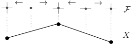
Figure 2: An abstract sketch of the force cosheaf $\mathcal{F}$ over $\mathbb{R}^{2}$ is pictured. The stalks of $\mathcal{F}$ are situated “above” the cells of $X$ with linear maps respecting incidence.

Although this initial paper focuses on the planar setting ($n=2$), we present the definitions in more generality to permit higher-dimensional graphic statics in future work.

Definition 16 (Force Cosheaf).

Let $(X,p)$ be a diagram with injective realization. The force cosheaf $\mathcal{F}$ over $(X,p)$ has stalks that keep track of internal and external forces as follows. Each vertex $v$ has stalk $\mathcal{F}_{v}=\mathbb{R}^{n}$ thought of as a tangent space at $p(v)$ with unit basis vectors $\partial_{i}=\partial/\partial x_{i}$. Each edge $e$ has stalk $\mathcal{F}_{e}=\mathbb{R}$ thought of as a 1-D space tangent to the edge with basis vector $\partial_{t}$. For an edge $e$ connecting vertices $u$ and $v$, the map $\mathcal{F}_{e\rhd v}$ sends the unit basis vector $\partial_{t}$ to the unit normalization of the vector $p(v)-p(u)$. All stalks over higher-dimensional cells of $X$ vanish.

Remark 17.

One can profitably think of the geometric realization of each edge $e$ with endpoints $u\lhd e$ and $v\lhd e$ as the straight interval passing through the points $p_{v}$ and $p_{u}$. From this perspective, the stalk $\mathcal{F}_{e}$ can be thought of as the 1-D vector subspace ${\bf e}=\text{span}\{p_{v}-p_{e}\}$ of $\mathbb{R}^{n}$ parallel to the realization of $e$ induced by $p$. For an incident vertex $v$, the map $\mathcal{F}_{e\rhd v}$ is the inclusion of this subspace ${\bf e}$ into $\mathbb{R}^{n}=\mathcal{F}_{v}$, cf. the inclusion of the tangent space of a submanifold into the ambient manifold. See Example 32 for an instance where this perspective is useful.

The stalks represent forces applied at the joints (vertex stalks) and axial forces or stresses along the linkage element (edge stalks). The extension maps record how axial forces are distributed to the pin joints. Since $C_{i}\mathcal{F}=0$ for $i>1$, there are at most two non-zero homologies, determined by the boundary map $\partial:C_{1}\mathcal{F}\to C_{0}\mathcal{F}$ : the kernel of $\partial$, $H_{1}\mathcal{F}$, and the cokernel of $\partial$, $H_{0}\mathcal{F}$. The chains and homologies of $\mathcal{F}$ have the following useful interpretations in structural mechanics.

• Each 0-chain in $C_{0}\mathcal{F}$ is a distribution of static loads applied to vertices, i.e., a force vector in $\mathbb{R}^{n}$ applied to each vertex.

• Each 1-chain in $C_{1}\mathcal{F}$ is a distribution of internal axial forces, or stresses over the edges. The sign of this stress value in combination with the local orientation of the edge determines whether the stress is a tension (positive) or compression (negative).

• The boundary map $\partial:C_{1}\mathcal{F}\to C_{0}\mathcal{F}$ distributes the forces resulting from internal stresses over edges to adjacent vertices, summing at each vertex.

• The 1st homology $H_{1}\mathcal{F}=\ker\partial$ is the space of axial self stresses or equilibrium stresses of the truss. Each self stress satisfies an equilibrium equation over vertices, resulting in a net-zero force everywhere. For example, Figure 3 portrays a self-stressed truss.

• The 0th homology $H_{0}\mathcal{F}=\textrm{coker}\ \partial$ is the space of constrained degrees of freedom of vertices. These are assignments of forces to vertices that cannot result from tensile or compressive force within edges. These vertex forces then must instead impart infinitesimal accelerations to the structure: rotations, translations, or mechanisms: see Section 3.2.

We emphasize that struture and homology of $\mathcal{F}$ are highly dependent on the geometry of the diagram $(X,p)$. Varying the realization $p$ will change the force cosheaf, even if the topology of $X$ does not change. This is why, in the context of graphic statics, $(X,p)$ – the form diagram – is the crucial object of study. The force cosheaf is a richer algebraic structure that reveals the deeper implications of the form diagram.

Example 18 (Rigidity).

The zeroth homology detects rigidity. A diagram $(X,p)$ in $\mathbb{R}^{n}$ is rigid if there are no mechanisms – that is, if the only nonzero infinitesimal accelerations generate the special Euclidean group of rotations and translations. By the above interpretation of the force cosheaf homology, the diagram is rigid if and only if the dimension of $H_{0}\mathcal{F}$ is $\binom{n+1}{2}$, the dimension of the special Euclidean group of global translations and rotations in $n$ dimensional space. For example, an $n$-simplex realized in $\mathbb{R}^{n}$ with generic vertex coordinates is rigid as well as Figure 3. For non-rigid graphs, other generators of $H_{0}\mathcal{F}$ correspond to mechanisms.

Figure 3: A diagram $(X,p)$ is pictured where $\dim C_{0}\mathcal{F}=10$ and $\dim C_{1}\mathcal{F}=8$. The boundary map is not injective, with kernel spanned by the cycle that takes values $1$ on the four outside edges (tension) and takes values $-\sqrt{2}$ on the four interior edges (compression). This 1-cycle is a generator of $H_{1}\mathcal{F}\cong\mathbb{R}$.

3.2 The Linkage Sheaf

The linear dual of the force cosheaf is what we will call the linkage sheaf modeling the kinematics of a bar-and-joint linkage. The principle of virtual work implies that displacements are dual to forces and that the displacement coboundary map $\delta$ is the adjoint of the force boundary map $\partial^{\vee}$ [16].

Definition 19 (Linkage Sheaf).

The linkage sheaf $\mathcal{F}^{\vee}$ is the linear dual of the force cosheaf $\mathcal{F}$. Again, fixing a diagram $(X,p)$, vertex stalks $\mathcal{F}^{\vee}_{v}$ are dual spaces $(\mathbb{R}^{n})^{\vee}$ with basis 1-forms $dx_{i}$; the edge stalks are one-dimensional dual spaces $\mathcal{F}^{\vee}_{e}\cong\mathbb{R}^{\vee}$ with basis $dt$, and all stalks over higher dimensional cells vanish. For each edge $e$ between $u$ and $v$, the restriction map $\mathcal{F}^{\vee}_{v\lhd e}:(\mathbb{R}^{n})^{\vee}\to{\mathbb{R}}^{\vee}$ is the linear dual of the map $\mathcal{F}_{v\lhd e}:\mathbb{R}\to\mathbb{R}^{n}$, sending a covector $\alpha\in(\mathbb{R}^{n})^{\vee}$ at $v$ to the multiple of $dt$ with coefficient $\alpha(p_{e})$ where $p_{e}$ is the unit normalization of the vector $[u:e](p_{u}-p_{v})$.

If one thinks of the force cosheaf as having a map $\mathcal{F}_{e\rhd v}$ given by the inclusion of the subspace ${\bf e}$ “parallel” to the geometric edge into $\mathbb{R}^{n}$, then the linkage sheaf map $\mathcal{F}_{v\lhd e}:(\mathbb{R}^{n})^{\vee}\to{\bf e}^{\vee}$ is its linear dual.

• The space of 0-cochains $C^{0}\mathcal{F}^{\vee}$ consists of infinitesimal displacements of vertices in $\mathbb{R}^{n}$.

• The space of 1-cochains $C^{1}\mathcal{F}^{\vee}$ is the space of axial extensions and contractions. Normalizing by the length of each edge gives the strain.

• The coboundary map $\partial^{\vee}:C^{0}\mathcal{F}^{\vee}\to C^{1}\mathcal{F}^{\vee}$ computes the infinitesimal or 1st-order changes in the lengths of edges resulting from a given displacement of the truss vertices.

• The 0th cohomology $\ker\partial^{\vee}=H^{0}\mathcal{F}^{\vee}$ consists of constrained stiff displacements assigned to vertices that preserve edge length. Each constrained displacement rotates or translates the linkage while those edges remain rigid.

• The 1st cohomology $H^{1}\mathcal{F}^{\vee}$ consists of equivalence classes of unrealizable axial deformations — those axial deformations that cannot result from movements of vertices. These can be thought of as strain measurement reading errors.

As these are cotangent spaces (duals to tangent spaces), the displacements to the vertices should be thought of as either infinitesimal or (using an exponential map) 1st-order terms in the expansion of the displacement. By Theorem 12, the cohomology of the linkage sheaf is isomorphic to the homology of the force cosheaf. This provides a useful way of re-interpreting each (co)homology.

Example 20 (Impossible Axial Deformation).

For the diagram pictured in Figure 3, it is impossible for the four interior edges to grow in length while the four outside edges shrink. This cocycle is a generator for $H^{1}\mathcal{F}^{\vee}$ and is dual to the self stress. This coincides with the isomorphism $H^{1}\mathcal{F}^{\vee}\cong H_{1}\mathcal{F}$ following Theorem 12.

3.3 Maxwell’s Rule and Euler Characteristic

Additional tools from algebraic topology enable elegant reformulations of principles in static analysis. One such tool is the classical Euler characteristic, adapted to cellular cosheaves.

Recall the elementary topological fact that for a finite polyhedral spherical surface $X$ with $|V|$ vertices, $|E|$ edges, and $|F|$ faces, the Euler characteristic $\chi\left(X\right)=|V|-|E|+|F|$ equals $+2$, independent of how the spherical surface is discretized. The reason for this is an elementary but fundamental result. For a finite sequence of finite-dimensional vector spaces $C=(C_{i})$, its Euler characteristic $\chi(C)$ is the alternating sum of dimensions of the vector spaces. In the context of a chain complex, there is an important and fundamental relationship to homology:

Lemma 21.

[65] The Euler characteristic of a chain complex $C=\left(C_{i}\right)$ and its homology $H=\left(H_{i}\right)$ agree:

$$\sum_{i}{\left(-1\right)^{i}\dim C_{i}}=\chi(C)=\chi(H)=\sum_{i}{\left(-1\right)^{i}\dim H_{i}},$$ (8)

This is why for a triangulated spherical surface $\chi=2$, since the classical homology of a cell complex comes from the constant cosheaf (Example 6) and this cosheaf has Euler characteristic given by $|V|-|E|+|F|$, while the homology of a sphere is $\dim H_{0}=\dim H_{2}=1$ and $\dim H_{k}=0$ for all other $k$. Lemma 21 also holds for the cohomology of a cochain complex (by simple duality).

When applied to the force cosheaf (or the linkage sheaf), one immediately generalizes Example 18 to obtain the classic Maxwell’s Rule [3]. The modern form for two dimensional trusses is given in [16] as

$$2|V|-|E|=3+|M|-|S|,$$ (9)

where $|M|$ is the number of linkage mechanisms, $|S|$ is the number of self-stresses, $|V|$ is the number of vertices of the truss, and $|E|$ is the number of its edges. The prevalence of differences suggests that this is related to Euler characteristic.

Theorem 22 (Maxwell’s Rule in dimension $n$).

Given a diagram $(X,p)$ in $\mathbb{R}^{n}$, the generalized Maxwell’s Rule holds:

$$n|V|-|E|=\binom{n+1}{2}+|M|-|S|$$ (10)

Proof.

Apply Lemma 21 to the force cosheaf, noting that in dimension $n$, the dimension of $H_{0}\mathcal{F}$ equals the sum of the number of the Euclidean motions ($n(n+1)/2$) plus the number of linkage mechanisms $|M|$. ∎

Dualization implies that the theorem holds as well for the linkage sheaf, which makes interpreting the linkage mechanisms clearer and gives an equivalence between the number of self-stresses and the number of unrealizable axial deformations.

3.4 Stiffness and the Sheaf Laplacian

The relationship between stress and strain is encoded in Hooke’s Law for ideal elastic elements. Under deformation, the strain within an axial element is proportional to its force output by its spring constant $\kappa_{e}$, parameterized by the edges $e$ of the diagram $X$. Multiplying by $\kappa_{e}$ determines an explicit isomorphism between the (one-dimensional) vector space of axial extensions and contractions of $e$ (i.e. $\mathcal{F}^{\vee}_{e}$) and the vector space of stresses of the element ($\mathcal{F}_{e}$). The quadratic form of this inner product $\langle a,b\rangle_{e}=\kappa_{e}ab$ on $\mathcal{F}_{e}^{\vee}$ represents the work done by a given axial deformation of the element. Using this inner product rather than the obvious one induced by the ambient space is useful as a way of determining weights for a sheaf Laplacian on the linkage sheaf $\mathcal{F}^{\vee}$ (recall Section 2.3). We begin with a simple classical example.

Example 23.

For a single edge $e$ in $\mathbb{R}^{2}$ between vertices at points $p(u)$ and $p(v)$, the component stiffness matrix $K_{e}$ for this element is typically defined by an equation like

$$K_{e}=\kappa_{e}\small\begin{bmatrix}\cos^{2}(\theta)&\cos(\theta)\sin(\theta)&-\cos^{2}(\theta)&-\cos(\theta)\sin(\theta)\\ \cos(\theta)\sin(\theta)&\sin^{2}(\theta)&-\cos(\theta)\sin(\theta)&-\sin^{2}(\theta)\\ -\cos^{2}(\theta)&-\cos(\theta)\sin(\theta)&\cos^{2}(\theta)&\cos(\theta)\sin(\theta)\\ -\cos(\theta)\sin(\theta)&-\sin^{2}(\theta)&\cos(\theta)\sin(\theta)&\sin^{2}(\theta)\\ \end{bmatrix},$$ (11)

where $\theta$ is the angle at which the edge $e$ is inclined in the Euclidean plane. The total stiffness matrix is the block matrix $K$ comprised of sums of matrices $K_{e}$ over every edge.

The stiffness matrix is a symmetric linear operator that takes a vector of infinitesimal displacements of vertices to a vector of forces at the vertices. Another perspective is that, as a quadratic form, the stiffness matrix represents the infinitesimal work done by an infinitesimal displacement of the vertices, or, equivalently, that $\langle\xi,K\xi\rangle$ is (twice) the potential energy stored in the truss as a result of the deformation $\xi$.

We claim that the stiffness matrix is really the sheaf Laplacian of $\mathcal{F}^{\vee}$ with respect to the inner product given by the spring constants $\kappa_{e}$. This is simple to see from the perspective of the quadratic form, beginning with the observation that $\langle\xi,\Delta\xi\rangle=\langle\delta\xi,\delta\xi\rangle$. Since the coboundary $\delta$ computes the infinitesimal edge deformations given by vertex displacements, and the inner product computes (and sums) the work done by each edge deformation, this is precisely the work done on the truss by the vertex displacement $\xi$. One can also show this fact by computing the matrix entries of $\Delta$ and showing that they are equal to those of $K_{e}$ as defined above (11), but this is more tedious and less enlightening than the work-based proof.

This interpretation of the stiffness matrix as a weighted sheaf Laplacian allows for the following result, an immediate consequence of Theorem 15.

Corollary 24.

For $\xi_{0}\in C^{0}\mathcal{F}^{\vee}$ an initial condition of vertex displacements of a diagram $(X,p)$, the diffusion equation

$$\frac{d\xi}{dt}=-\Delta_{\mathcal{F}^{\vee}}\xi$$ (12)

with $\Delta_{\mathcal{F}^{\vee}}$ the sheaf Laplacian of $\mathcal{F}^{\vee}$, converges to a vertex displacement $\xi_{\infty}\in H^{0}\mathcal{F}^{\vee}$ representing a stiff displacement for which all members have zero internal force.

Utilizing mass and dampening matrices as well as the stiffness matrix, the wave equation is another legitimate model for truss dynamics.

3.5 The Position Sheaf

In Section 3.2 we saw how $H^{0}$ of the linkage sheaf $\mathcal{F}^{\vee}$ determines constrained stiff displacements of the truss. Under such an action, the truss is manipulated by a mechanism or global motion without extending edges. Here we consider the opposite: the space of deformations on a truss that only extend and contract edges, keeping them parallel. This space of parallel motions is captured by the cohomology of the following sheaf.

Definition 25 (Position Sheaf).

Suppose $(X,p)$ is a diagram in Euclidean space $\mathbb{R}^{n}$ with injective realization. The position sheaf $\mathcal{J}$ is built as follows. Consider the sheaf whose vertex stalks are the dual spaces $(\mathbb{R}^{n})^{\vee}$. Assign to each edge $e$ the stalk the quotient of $(\mathbb{R}^{n})^{\vee}$ by the subspace $\mathcal{F}^{\vee}_{e}={\bf e}^{\vee}$ from Definition 19. All higher dimensional cells have zero stalks. The restriction maps $\mathcal{J}_{v\lhd e}$ are precisely the projections onto these quotient spaces.

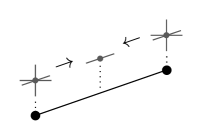
(a) Sketch of the linkage sheaf in $\mathbb{R}^{3}$

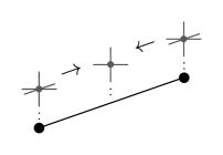
(b) Sketch of the position sheaf in $\mathbb{R}^{3}$

The cochain complex and the cohomology of $\mathcal{J}$ can be interpreted as follows.

• The 0-cochains $C^{0}\mathcal{J}$ are infinitesimal deformations, as per the linkage sheaf.

• The 1-cochains $C^{1}\mathcal{J}$ are systems of orthogonal deviations of edges with respect to the original realization $p$. Over an edge $u,v\lhd e$ in $(X,p)$, an element $o_{e}\in\mathcal{J}_{e}$ is a co-vector perpendicular (or quotient) to the edge. If one fixes a reference frame at one vertex $u$ and “looks down the edge” in $\mathbb{R}^{n}$, we let the co-vector $[u:e]o_{e}$ act on vertex $v$ by displacing it in the plane of view. No displacement of $v$ out of plane (or parallel to $e$) can be detected however. These 1-chains can be considered as 1-forms in the normal subspace to the edge. For small values of $o_{e}$, the small angle approximation $o_{e}=\sin(\theta)\sim\theta$ means we consider $o_{e}$ as a small rotation of the edge by $\theta$. This is pictured in Figure 5 (right).

• The coboundary $\delta:C^{0}\mathcal{J}\to C^{1}\mathcal{J}$ takes a deformation of $(X,p)$ and measures its induced orthogonal deviation over edges. Specifically, given $\xi\in C^{0}\mathcal{J}$, the coboundary $\delta\xi$ evaluated at edge $e$ describes the net orthogonal motion of $e$ under the realization $p+\xi$.

• The 0-cohomology $H^{0}\mathcal{J}$ consists of parallel extensions of $X$, deformations to vertices such that edges remain parallel to their original. For an orthogonal deviation $\xi\in H^{0}\mathcal{J}$, over an edge $u,v\lhd e$ and at a vector $x_{e}\in{\bf e}^{\perp}$ the co-vector $\xi_{v}-\xi_{u}$ takes value $(\xi_{v}-\xi_{u})(x_{e})=0$: thus, $\xi_{v}=\xi_{u}$, and the induced edges in the deformed diagram $(X,p+\xi)$ are parallel to those in $(X,p)$.

• The cohomology $H^{1}\mathcal{J}$ is the space of equivalence classes of impossible orthogonal deviations or impossible edge rotations. These are error assignments to edges which cannot result from any possible choice of vertex coordinates. Figure 6 depicts a prototypical cocycle.

Parallel deformations in $H^{0}\mathcal{J}$ are co-vectors and can be summed, resulting in a visual algebra of shape. For instance, if $\xi_{0},\xi_{1}\in H^{0}\mathcal{J}$ are two cocycles, the deformations can be added to the diagram $(X,p+\xi_{0}+\xi_{1})$. Moreover the realization $p$ (differentially $dp$) itself is a parallel deformation, scaling with respect to the origin $(X,p)$ to the diagram $(X,p+dp)$. To better understand the vector space we can observe the realization of infinitesimals $(X,\xi)$ for $\xi\in H^{0}\mathcal{J}$. There is an isomorphism between diagrams of the form $(X,\xi)$ and diagrams of the form $(X,p+\xi$). This is justified by canonical isomorphisms between tangent spaces $T_{p_{v}}\mathbb{R}^{n}$ and the base manifold $\mathbb{R}^{n}$. Figure 5 (left) and (center) depicts this duality between infinitesimal rotations and scalings.

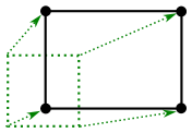
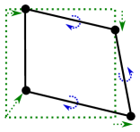
Figure 5: In an example with $(X,p)$ a square, the position sheaf cochain complex has $C^{0}\mathcal{J}$ of dimension eight and $C^{1}\mathcal{J}$ of dimension four with a surjective coboundary map. Two generators of parallel realizations in $H^{0}\mathcal{J}$ translate the square in space while the two other generators change the aspect ratio of the square, fully describing all rectangles in the plane (left). Where a cocycle $r\in H^{0}\mathcal{J}$ deforms the diagram $(X,p)$ to $(X,p+r)$ (left), one can instead depict $r$ as a diagram of infinitesimals (center), as a realization of $X$ in its own right $(X,r)$. In $C^{1}\mathcal{J}$, each 1-cochain measures the edge rotation of an alternative diagram relative to original $(X,p)$ (right). For the square, $H^{1}\mathcal{J}=0$, meaning every possible orthogonal edge deviation in $C^{1}\mathcal{J}$ is the coboundary of some choice of vertex coordinates in $C^{0}\mathcal{J}$. A cochain is drawn (right), with orthogonal edge deformations drawn more perceptibly as (small) rotations.

Example 26 (Impossible Edge Rotation).

Suppose $(X,p)$ is the form diagram in Figure 3. In constructing alternative parallel realizations, notice the diagonal edges lock the aspect ratio of the outer square. Consequently the vector space $H^{0}\mathcal{J}$ consists of two translations and one scaling dimension. The Euler characteristic formula (8) for sheaves indicates that $H^{1}\mathcal{J}$ is one dimensional, with a generator pictured in Figure 6 (left). Just as mechanisms of a truss cannot be resisted by truss members (inducing motion), impossible edge rotations cannot be realized by nodal positions.

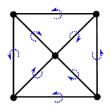
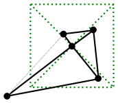
Figure 6: An impossible infinitesimal edge rotation, illustrating an element of $H^{1}\mathcal{J}$, is sketched (left). To see this as an impossible class, first fix the center vertex. The four diagonal edges act by rotating the four corner vertices clockwise. No matter how one contracts or extends the diagonal edges, at least one exterior edge must rotate clockwise as well (right). Specifying the outside edges to all rotate counterclockwise is a contradiction – an impossible requirement.

Example 27 (Self Shear).

The position sheaf has its own linear dual $\mathcal{J}^{\vee}$. For $\mathcal{J}$ a position sheaf over the diagram $(X,p)$, the cosheaf $\mathcal{J}^{\vee}$ has edge stalks ${\bf e}^{\perp}\cong\mathbb{R}^{n-1}$ over edges, with extension maps embeddings $\mathcal{J}^{\vee}=E_{e^{\perp}}$ from these perpendicular subspace into $\mathbb{R}^{n}$ vertex stalks.

Similar to the force cosheaf, the homology $H_{1}\mathcal{J}^{\vee}$ has interpretation as a space of self-shear stresses. Here, the values of a stalk $\mathcal{J}^{\vee}_{e}\cong{\bf e}^{\perp}$ is the space of shear forces perpendicular to the member $e$. This equilibrium of these forces is self-shear, where no edge is loaded with any axial force.

Example 28 (Position Sheaf Laplacian).

Akin to the stiffness matrix in Section 3.4, the sheaf Laplacian of the position sheaf $\Delta_{\mathcal{J}}$ has interesting properties. Although spring constants can be introduced, consider the unweighted sheaf Laplacian $\Delta_{\mathcal{J}}=\delta\circ\delta$. For the position sheaf $\mathcal{J}$ over a reference diagram $(X,p)$, the diagram $(X,p+\xi_{t})$ with arbitrary initial realization $\xi_{0}\in C^{0}\mathcal{J}$ undergoes transformation under the differential equation

$$\frac{d\xi}{dt}=-\Delta_{\mathcal{J}}\xi.$$ (13)

The realization displacements $\xi_{t}$ converge to $\xi_{\infty}\in H^{0}\mathcal{J}$, a parallel realization to $p$. The limit diagram $(X,p+\xi_{\infty})$ is the closest diagram to $(X,p+\xi_{0})$ parallel to $(X,p)$ in the sense that $\xi_{\infty}$ minimizes the expression [64]

$$\|\xi_{\infty}-\xi_{0}\|=\sqrt{\sum_{v\in V}\left\|\xi_{\infty}(v)-\xi_{0}(v)\right\|^{2}}.$$ (14)

Figure 7: The action of the position sheaf Laplacian (derived from Figure 3) is pictured on a diagram with arbitrary realization $(X,p+\xi_{0})$. Under the heat equation (13), the realization exponentially converges to that of the limit diagram $(X,p+\xi_{\infty})$ parallel to that of Figure 3.

Example 29 (Maxwell Dualized).

Recall from Section 3.3 that the classical Maxwell Rule follows from the invariance of the Euler characteristic under (co)homology of the force cosheaf or the linkage sheaf. The same can be directly applied to the position sheaf and its dual cosheaf, with corresponding interpretations. We leave this variation of the Maxwell Rule to the curious reader as an illustrative exercise.

3.6 Maps Between Cosheaves

Any given cosheaf is best understood in relation to other cosheaves. These connections are algebraically formed by distributed linear maps between stalks, subject to constraints ensuring the consistency of the transmitted data.

Definition 30 (Cosheaf Map).

For two cosheaves $\mathcal{K}$ and $\mathcal{L}$ over the same cell complex $X$, a cosheaf map $\phi:\mathcal{K}\to\mathcal{L}$ consists of a collection of linear maps $\{\phi_{c}:\mathcal{K}_{c}\to\mathcal{L}_{c}\}$ on stalks satisfying, for each pair of adjacent cells $c\lhd d$, the following commutativity condition:

(15)

Commutativity here means the compositions of maps $\mathcal{K}_{d}\to\mathcal{L}_{c}$ are path-independent.

Each cosheaf map $\phi:\mathcal{K}\to\mathcal{L}$ induces a map between chain complexes $\phi:C\mathcal{K}\to C\mathcal{L}$ by combining all stalk-wise linear component maps. A cosheaf morphism $\phi$ is injective, surjective, or an isomorphism if each of its component maps $\phi_{c}$ are.

Intuition from linear algebra holds: an injective cosheaf map $\phi:\mathcal{K}\to\mathcal{L}$ can be thought of as a “sub-cosheaf” – an inclusion of one data structure into another. To model the data in $\mathcal{L}$ that is “orthogonal” to $\mathcal{K}$, one builds the quotient cosheaf $\mathcal{K}/\mathcal{L}$ with stalks being quotient vector spaces $\left(\mathcal{L}/\mathcal{K}\right)_{c}=\mathcal{L}_{c}/\mathcal{K}_{c}$ with $c$ ranging over all cells. Extension maps over incident cells $c\lhd d$ are derived from the larger cosheaf $\mathcal{L}$ taking the form

$$\mathcal{L}/\mathcal{K}_{d\rhd c}(x+\textrm{im}\,\phi_{d})=\mathcal{L}_{d\rhd c}(x)+\mathcal{L}_{d\rhd c}(\textrm{im}\,\phi_{d})=\mathcal{L}_{d\rhd c}(x)+\textrm{im}\,\phi_{c}$$ (16)

where the second equality comes from the commutativity of (15). One can think of $\mathcal{L}/\mathcal{K}$ as encoding the quotient to $\mathcal{K}$ inside of $\mathcal{L}$, with a cosheaf projection map $\pi:\mathcal{L}\to\mathcal{L}/\mathcal{K}$.

The relationship between the cosheaves $\mathcal{K},\mathcal{L}$ and $\mathcal{L}/\mathcal{K}$ is especially significant.

Definition 31 (Exact Sequences).

A sequence of vector spaces

$$\dots\to V_{3}\to V_{2}\to V_{1}\to V_{0}\to V_{-1}\to\dots$$ (17)

is said to be exact if, at each term, the image of the incoming linear transformation is precisely the kernel of the outgoing linear transformation. Equivalently, the sequence (17) is a chain complex whose homology completely vanishes.

In the special case that (17) is non-zero in at most three incident terms, one rewrites this as a short exact sequence

$$0\to V_{2}\to V_{1}\to V_{0}\to 0.$$ (18)

It follows [65] that there are isomorphisms $V_{1}\cong V_{0}\oplus V_{2}$ and $V_{0}\cong V_{1}/V_{2}$. In the case of cosheaves $\mathcal{K},\mathcal{L}$ and $\mathcal{L}/\mathcal{K}$ as above, one has the short exact sequence of cosheaves

$$0\to\mathcal{K}\xrightarrow{\phi}\mathcal{L}\xrightarrow{\pi}\mathcal{L}/\mathcal{K}\to 0.$$ (19)

Over each cell $c$, $\phi_{c}$ is injective, $\pi_{c}$ is surjective, and $\textrm{im}\,\phi_{c}\cong\ker\pi_{c}$. One has an isomorphism of cosheaves $\mathcal{L}\cong\mathcal{K}\oplus\mathcal{L}/\mathcal{K}$, in which the data of $\mathcal{L}$ is subdivided into its constituent components parallel and orthogonal to $\mathcal{K}$.

Consolidating cosheaf maps, a short exact sequence of cosheaves induces a short exact sequence of cosheaf chain complexes

$$0\to C\mathcal{K}\xrightarrow{\phi}C\mathcal{L}\xrightarrow{\pi}C\mathcal{L}/\mathcal{K}\to 0.$$ (20)

These chain complexes yield the canonical long exact sequence in cosheaf homology

$$\cdots\rightarrow H_{i+1}\mathcal{L}/\mathcal{K}\xrightarrow{\vartheta}H_{i}\mathcal{K}\xrightarrow{\phi}H_{i}\mathcal{L}\xrightarrow{\pi}H_{i}\mathcal{L}/\mathcal{K}\xrightarrow{\vartheta}H_{i-1}\mathcal{K}\rightarrow\cdots$$ (21)

where $\vartheta$ here are called connecting homomorphisms. This sequence is exact as a sequence of vector spaces.

The various maps in the long exact sequence of homology (21) can be constructed rigorously. The induced linear maps $\phi$ and $\pi$ are the same as they are in the chain complex setting (20), only evaluated on homology classes.

For the reader who may not be familiar with methods from homological algebra, we briefly outline the construction of the connecting homomorphisms $\vartheta$ in sequence (21) here [65]. A homology class in $H_{i}\mathcal{L}/\mathcal{K}$ is represented by a cycle in $C_{i}\mathcal{L}/\mathcal{K}$. It can be shown that $\vartheta$ maps this representative to a chain in $C_{i-1}\mathcal{K}$ by the following procedure, outlined in diagram (22). The preimage of a cycle in $C_{i}\mathcal{L}/\mathcal{K}$ by $\pi$ is a chain in $C_{i}\mathcal{L}$, to which the boundary map of $\mathcal{L}$ is applied. The preimage of this chain in $C_{i-1}\mathcal{L}$ is an element of $C_{i-1}\mathcal{K}$, which can be shown to be a cycle, hence a homology class in $H_{i-1}\mathcal{K}$.

(22)

Furthermore, incorporating $\vartheta$ it can be shown the sequence (21) truly is exact.

Example 32 (Geometry of Axial Forces).

The edge-stalks of the force cosheaf $\mathcal{F}$ can, by abuse of notation, be thought of as edge-parallel subspaces of the vertex stalks $\mathbb{R}^{n}$. Consequently, $\mathcal{F}$ can be embedded as a sub-cosheaf of the larger constant cosheaf $\overline{\mathbb{R}^{n}}$. This latter constant cosheaf describes the ambient Euclidean space of forces.

Suppose $\mathcal{F}$ is the force cosheaf over a two dimensional cell complex $X$ realized in $\mathbb{R}^{n}$. There is an injective map $\phi:\mathcal{F}\to\overline{\mathbb{R}^{n}}$ between cosheaves where $\phi_{v}$ is the identity over vertices and $\phi_{e}$ is the embedding map $E_{e}:\mathbb{R}\cong{\bf e}\to\mathbb{R}^{n}$ of the edge stalk into $\mathbb{R}^{n}$. This cosheaf map $\phi_{f}=0$ is trivial over faces.

From the injective cosheaf map $\phi$, the quotient $\overline{\mathbb{R}^{n}}/\mathcal{F}$ is the cosheaf of complementary data in $\mathbb{R}^{n}$. The stalks of this cosheaf are comprised of full $\mathbb{R}^{n}$ data over faces and orthogonal data ${\bf e}^{\perp}$ along edges, with trivial data over vertices. Summarizing the relationships between these is a commutative diagram of stalks over every triplet of incident cells $v\lhd e\lhd f$.

(23)

Here, $P_{e^{\perp}}$ is the projection map to the equivalence class $x\to x+{\bf e}\in\mathbb{R}^{n}/{\bf e}$ in the quotient. This can be regarded as projecting to the orthogonal subspace ${\bf e^{\perp}}$, utilizing an inner product on stalks.

Choosing $X$ to be a polyhedral sphere $S^{2}$, the Poincaré dual of the cosheaf $\mathbb{R}^{n}/\mathcal{F}$ is a position sheaf over the dual polyhedral sphere $\tilde{X}$. Interpreting face stalks of $\overline{\mathbb{R}^{n}}/\mathcal{F}$ to be the coordinates of Poincaré dual vertices in Euclidean space, this forms a position sheaf over $\tilde{X}$.

4 Planar Graphic Statics

At heart graphic statics is visual; hidden internal axial forces within truss members are put on full display in reciprocal diagrams. This phenomenon is most clearly seen with planar trusses, where a spherical cell complex is projected to the plane.

Figure 8: Force diagrams dual to a form diagram are pictured. The form diagram (left) has two degrees of self stress generated by holding the covered edges in tension or compression. One type of dual diagram (center) emerges from specifying these forces to have the same sign. Another type of dual diagram (right) comes from having one edge in tension and one in compression. As force configurations can be linearly added over a truss, force diagrams can likewise be added, giving a “structural algebra” of graphs.

4.1 2D Planar Duality

Here we formulate graphic statics algebraically. From Example 32, over a form diagram $(X,p)$ in $\mathbb{R}^{2}$ there is a short exact sequence of cosheaves

$$0\to\mathcal{F}\xrightarrow{\phi}\overline{\mathbb{R}^{2}}\xrightarrow{\pi}\overline{\mathbb{R}^{2}}/\mathcal{F}\to 0$$ (24)

where $\mathcal{F}$ is the force cosheaf and $\overline{\mathbb{R}^{2}}$ the constant cosheaf with $\mathbb{R}^{2}$ stalks. The homological algebra of these cosheaves is graphic statics in its abstract form. With the cell complex $X$ a topological sphere $S^{2}$, the Poincaré dual sheaf to $\overline{\mathbb{R}^{2}}/\mathcal{F}$ takes the form of a position sheaf over $\tilde{X}$ whose structure is determined by the form diagram $(X,p)$. For brevity, we use a more concise notation $\mathcal{G}=\overline{\mathbb{R}^{2}}/\mathcal{F}$ .

With the interpretations of Section 3.5, an element of the stalk $\tilde{\mathcal{G}}_{\tilde{f}}$ gives coordinates for the vertex $\tilde{f}$ dual to the face $f$. A cochain of $C^{0}\tilde{\mathcal{G}}$ is then the data of a realization $q$ of $\tilde{X}$ (by abuse of notation, interchanging deformations and realizations of diagrams, discussed in Figure 5). To be a cocycle, $q$ must satisfy a cocycle condition property over dual edges. For coordinates $q_{\tilde{f}}$ and $q_{\tilde{g}}$ of dual vertices incident to an edge $\tilde{f},\tilde{g}\lhd\tilde{e}$, the difference between these coordinates must be in the subspace ${\bf e}\subset\mathbb{R}^{2}$. Under these constraints, a realization $q$ would set a dual edge $\tilde{e}$ parallel to its primal counterpart $e$ in the diagram $(X,p)$. Cohomology classes of $H^{0}\tilde{\mathcal{G}}$ are dual realizations specifying parallel dual diagrams $(\tilde{X},q)$.

The short exact sequence of cosheaves (24) above has a corresponding long exact homology sequence (21). Due to the trivial stalks of $\mathcal{F}$ and $\mathcal{G}$, this long exact sequence is simplified by two zero homology spaces $H_{2}\mathcal{F}$ and $H_{0}\mathcal{G}$. Further simplifications are made by considering the homology of the constant cosheaf. These homology spaces are determined by the base topology of $S^{2}$, namely $\dim H\overline{\mathbb{R}^{2}}=2\dim HS^{2}$. In particular $H_{1}\overline{\mathbb{R}^{2}}=0$ is zero, splitting the long exact sequence into two.

$$0\to\mathbb{R}^{2}\xrightarrow{\pi}H_{2}\mathcal{G}\xrightarrow{\vartheta}H_{1}\mathcal{F}\to 0$$ (25)

$$0\to H_{1}\mathcal{G}\xrightarrow{\vartheta}H_{0}\mathcal{F}\xrightarrow{\phi}\mathbb{R}^{2}\to 0$$ (26)

where $\vartheta$ are connecting homomorphisms. These two homology sequences are at the heart of two-dimensional graphic statics. The first encodes the algebraic relationship between axial self stresses and dual realizations. The second links mechanical degrees of freedom to dual impossible rotations.

Theorem 33 (Planar Force and Form [3, 15]).

Let $(X,p)$ be a spherical form diagram in $\mathbb{R}^{2}$. There is a bijection between self stresses $a\in H_{1}\mathcal{F}$ and parallel force diagrams $(\tilde{X},q)$ with realization $q\in H^{0}\tilde{\mathcal{G}}$ up to global translation satisfying the condition that over each edge of $X$ bounded by two faces $e\lhd f,g$, the force $w_{e}$ is equal to the oriented length $[e:f](q_{\tilde{f}}-q_{\tilde{g}})$ of the dual edge $\tilde{e}$.

Proof.

This theorem is a consequence of the exactness of sequence (25). We walk through each step of the process to fully develop the correspondence.

By exactness at $H_{2}\overline{\mathbb{R}^{2}}\cong\mathbb{R}^{2}$ the map $\pi$ is injective, and by exactness at $H_{1}\mathcal{F}$ the map $\vartheta$ is surjective. In particular, for any self stress $a\in H_{1}\mathcal{F}$ over $X$ there must be a realization $q\in H^{0}\tilde{\mathcal{G}}$ as a preimage of $\vartheta$. For any two preimages $q,r$ of $w$ the realization $q-r$ is in the kernel of the connecting homomorphism $\vartheta$. Exactness at $H_{2}\mathcal{G}$ states that the kernel of $\vartheta$ is equal to the image of $\pi$, so $q-r$ itself has a preimage by $\pi$ in $H_{2}\overline{\mathbb{R}^{2}}\cong\mathbb{R}^{2}$ a global translation vector. Subsequently, the difference of realizations $q-r$ is a global translation of all dual vertex coordinates of $\tilde{X}$. This describes the bijection up to global translation.

The value of the bijection follows from the construction of the connecting homomorphism $\vartheta$, outlined by line (22). The preimage of $q$ by $\pi$ is a cycle in $C_{2}\overline{\mathbb{R}^{2}}$, where it is mapped by the boundary map of the cosheaf $\overline{\mathbb{R}^{2}}$ into $C_{1}\overline{\mathbb{R}^{2}}$. There it takes value $[e:f](q_{f}-q_{g})$ over edge $f,g\rhd e$, which, over the dual diagram is the difference in coordinates $[\tilde{f}:\tilde{e}](q_{\tilde{f}}-q_{\tilde{g}})$ over the dual edge $\tilde{e}$. This is the value of the self-stress $w_{e}$ over the primal edge $e$.

In this way, the dual edge $\tilde{e}$ is not only parallel to $e$ but its length is determined by the cycle $w\in H_{1}\mathcal{F}$. The direction and magnitude of the force vector $w_{e}$ is equal to the edge $\tilde{e}$ as realized by $q\in H^{0}\tilde{\mathcal{G}}$. ∎

Theorem 33 describes the nature of the isomorphism $H^{0}\tilde{\mathcal{G}}/\mathbb{R}^{2}\cong H_{1}\mathcal{F}$ following the exact sequence of vector spaces (25). The second exact sequence (26) gives a similar theorem linking two other homological spaces. Recall that an impossible edge rotation is an edge assignment that cannot possibly result from any realization even allowing for free axial extension of dual edges. Here, impossible dual edge rotations of the reciprocal diagram $(\tilde{X},q)$ are linked to mechanical freedom of the primal.

Theorem 34 (Mechanics and Impossible Rotations in $\mathbb{R}^{2}$ ).

Let $(X,p)$ be a spherical diagram realized in $\mathbb{R}^{2}$ and let $(\tilde{X},q)$ be a parallel reciprocal diagram. There is a bijection correspondence between impossible edge rotations of $(\tilde{X},q)$ and the mechanisms and global rotations of $(X,p)$.

Proof.

Every impossible edge rotation of $\tilde{X}$ is an element of $H^{1}\tilde{\mathcal{G}}\cong H_{1}\mathcal{G}$. The map $\vartheta$ in exact sequence (26) is injective, meaning taking the influence of dual edge rotations and summing them at vertices activates a degree of freedom of $X$ in $H_{0}\mathcal{F}$. The map $\phi:H_{0}\mathcal{F}\to\mathbb{R}^{2}$ is surjective, meaning global translations are always degrees of freedom of $X$.

By exactness at the middle vector space $H_{0}\mathcal{F}$, the image of $\vartheta$ in $H_{0}\mathcal{F}$ is isomorphic to the kernel of $\phi$, which consists of degrees of freedom of $X$ which have no net global translation effect. Because any linear map is an isomorphism onto its image, $H^{1}\tilde{\mathcal{G}}$ is isomorphic to this space of non-translational degrees of freedom, equivalent to the space of mechanisms and global rotations of $X$. ∎

A mechanism or global rotation $x\in H_{0}\mathcal{F}$ applied to the structure $X$ rotates at least some of the edges of $(X,p)$. These edge rotations of may be transferred to the reciprocal $(\tilde{X},q)$ after accounting for the sign of dual edges. By Theorem 33, each dual edge $\tilde{e}$ of $(\tilde{X},q)$ corresponds to a primal edge $e$ of $(X,p)$ in tension or in compression. It is a technical point, but if an edge $e$ is in tension (under the convention that tension is a negative value over edges), its dual $\tilde{e}$ is realized in reverse, inverted in the force diagram. Consequently, cycles or cocycles drawn over mirrored dual edges $\tilde{e}$ are also drawn mirrored. A clockwise rotation over an edge in tension transfers to a counterclockwise rotation over its counterpart.

Example 35 (Reciprocal Rotations).

Suppose that $(X,p)$ is the form diagram in Figure 3. This truss has two translational degrees of freedom and one rotational degree of freedom. Under a counterclockwise rotation around the central node pictured in Figure 9 (left), all edges rotate counterclockwise as well. This form diagram has one degree of self-stress holding the internal four edges in tension. By Theorem 33, this self stress determines a parallel realization of the dual cell complex $\tilde{X}$, pictured (center) in Figure 9.

Because the internal four diagonal edges (left) are loaded in tension, their dual edges (center) have their sign reversed. The rotations of these four diagonal edges on the dual diagram (center) are reversed, rotating clockwise instead. This is an impossible edge rotation of the force diagram – an element of $H^{1}\tilde{\mathcal{G}}$ over $\tilde{X}$. This matches with previously found impossible rotation configuration of Figure 6.

4.2 Plane Reciprocity

The concept of “reciprocity” here refers to interchanging the roles of the form diagram and force diagram, reversing the relationship between the two. The self stresses of any form diagram determine dual parallel realizations according to Theorem 33. A dual diagram $(\tilde{X},q)$ itself is a diagram in $\mathbb{R}^{2}$, with all the characteristics that the prior $X$ had. Namely $(\tilde{X},q)$ may have self stresses and mechanisms, governed by the force cosheaf over it.

We may proceed with constructing the force cosheaf over $\tilde{X}$, but we would like to do so with respect to the cosheaves $\mathcal{F},\overline{\mathbb{R}^{2}},\mathcal{G}$ previously developed in Section 4.1. In this way, the homological properties of the force diagram can be interconnected to those of the form diagram. Here, we introduce the technique of rotating dual realizations. For $q$ an parallel dual realization in $H^{0}\tilde{G}$, let $q^{\prime}$ denote the same realization of $\tilde{X}$ rotated one quarter turn in the plane. By employing $q^{\prime}$, dual edges would be realized perpendicular to their counterparts in the form diagram $(X,p)$. The benefit is that the cosheaf $\tilde{\mathcal{G}}^{\vee}$ is the force cosheaf over $(\tilde{X},q^{\prime})$. Respecting the duality between reciprocal force and form diagrams, we call $\tilde{\mathcal{G}}^{\vee}$ the reciprocal cosheaf to $\mathcal{G}$.

Lemma 36.

Let $(X,p)$ be a diagram in $\mathbb{R}^{2}$. The force cosheaf $\mathcal{F}$ and the linear dual of the position sheaf $\mathcal{J}^{\vee}$ are isomorphic.

Proof.

We construct a cosheaf isomorphism $\mu:\mathcal{F}\to\mathcal{J}^{\vee}$. Over edges $\mu$ is set to the identity transformation (taking vectors to linear functionals) and is a quarter turn over vertex stalks. Over incident edges and vertices $v\lhd e$, the following diagram commutes

(27)

where $\mu_{v}$ maps the subspace parallel to the edge ${\bf e}\subset\mathbb{R}^{2}$ to the perpendicular subspace ${\bf e^{\perp}}\subset\mathbb{R}^{2}$ by one-quarter turn (either clockwise or counter-clockwise, but consistent across all vertices). ∎

The technique of rotating vector values has been previously utilized to show the equivalence of rotations and (scaling) of a structure about the center of rotation [60]. This is evident in Figure 9 (left) and (right).

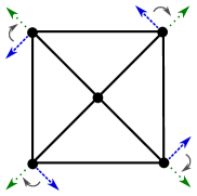
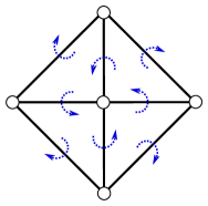
Figure 9: The truss $(X,p)$ from Figure 3 is rotated counterclockwise (left). This system of edge rotations on $(X,p)$ can be transferred to the dual diagram $(\tilde{X},q)$ (center). Rotating the chain (left) results in a parallel deformation (right).

Both parallel and perpendicular drawing conventions $q$ and $q^{\prime}$ of $\tilde{X}$ have been widely utilized [61]. Where dual edges are drawn parallel is known as the Cremona convention while where dual edges are drawn perpendicular is known as Maxwell’s convention.

Note the sheaf $\tilde{\mathcal{G}}$ has been predetermined to be the position sheaf over $\tilde{X}$ with respect to a realization $q$ parallel to $p$. By Lemma 36, its reciprocal $\tilde{\mathcal{G}}^{\vee}$ is the force cosheaf over $\tilde{X}$ with respect to the realization $q^{\prime}$ after rotating dual vertex coordinates. The reciprocal cosheaf exact sequence to sequence (24) is

$$0\to\tilde{\mathcal{G}}^{\vee}\xrightarrow{\pi^{\vee}}\overline{\mathbb{R}^{2}}\xrightarrow{\phi^{\vee}}\tilde{\mathcal{F}}^{\vee}\to 0$$ (28)

where $\overline{\mathbb{R}^{2}}$ is the constant cosheaf over $\tilde{X}$. Note that the adjoint maps not only flip the domain and codomains of linear incidence maps internal to (co)sheaves, but also flip the direction of linear (co)sheaf maps in the exact sequence.

With $\tilde{\mathcal{G}}^{\vee}$ the force cosheaf over $(\tilde{X},q^{\prime})$ and $\overline{\mathbb{R}^{2}}$ the two dimensional constant cosheaf, sequence (28) is fundamentally the same as the original cosheaf sequence (24), only over $\tilde{X}$ instead of $X$. Consequently, the double Poincaré dual sheaf $\tilde{\vphantom{\rule{1.0pt}{5.93056pt}}\smash{\tilde{\mathcal{F}}}}^{\vee}=\mathcal{F}^{\vee}$ is a position sheaf. The cohomology $H^{0}\mathcal{F}^{\vee}$ of consists of alternative realizations $p^{\prime}$ of $X$ parallel to $q^{\prime}$. These new diagrams $(X,p^{\prime})$ are thus perpendicular to the starting diagram $(X,p)$. This can also be seen from employing Lemma (36) directly from the original force cosheaf $\mathcal{F}$ over $(X,p)$.

The consequence of reciprocal and symmetric cosheaf sequences is this. Theorems 33 and 34 both apply in the reciprocal setting, from diagrams $(\tilde{X},q^{\prime})$ to $(X,p^{\prime})$. After rotating by one quarter turn, their relationship is the same as that of $(X,p)$ and $(\tilde{X},q)$. This symmetry allows the combination of the theorems combining their effects.

Theorem 37 (Reciprocal Relations).

Suppose $(X,p)$ and $(\tilde{X},q)$ are planar reciprocal diagrams over the plane $\mathbb{R}^{2}$, both with spherical $S^{2}$ regular cellular topology. There are isomorphisms between the following vector spaces:

• The space of mechanisms and global rotations of $(X,p)$.

• The space of parallel deformations of $(X,p)$ up to global translation.

• The space of impossible edge rotations over $(\tilde{X},q)$.

• The space of pure self shear stresses over $(\tilde{X},q)$.

• The space of axial self stresses over $(\tilde{X},q)$.

Proof.

We will prove the equivalence of (i) and (ii) on the diagram $(X,p)$, then prove the equivalences on the diagram $(\tilde{X},q)$.

By Lemma 36 and Theorem 12, the homology of the force cosheaf $\mathcal{F}$ over $(X,p)$ is isomorphic to the homology of the position sheaf $\mu\mathcal{F}^{\vee}$ over diagram $(X,p)$. Here, movement from a mechanism or rotation system (i) in $H_{0}\mathcal{F}$ is rotated by one quarter turn to form an parallel axial extension (ii) in $H^{0}\mu\mathcal{F}^{\vee}$. This latter homology space is equivalent to the space of parallel deformations of $p$ (ii). Removing the global translational degrees of freedom results in the expected isomorphism $H_{0}\mathcal{F}-\mathbb{R}^{2}\cong H^{0}\mu\mathcal{F}^{\vee}/\mathbb{R}^{2}$.

Recall that $\tilde{\mathcal{G}}$ is the position sheaf over $(\tilde{X},q)$. The space of impossible edge rotations $H^{1}\tilde{\mathcal{G}}$ is isomorphic to the space of pure shear stresses $H_{1}\tilde{\mathcal{G}}^{\vee}$ as described Example 27. Lemma 36 shows that this cosheaf $\tilde{\mathcal{G}}^{\vee}$ is isomorphic to the force cosheaf $\mu^{-1}\tilde{\mathcal{G}}^{\vee}$ over $(\tilde{X},q)$ after rotating by one quarter turn. This gives an isomorphism between the space (v) of axial self stresses $H_{1}\mu^{-1}\tilde{\mathcal{G}}^{\vee}$ and (iv).

Lastly, we connect the quantities over the two diagrams. Theorem 34 draws the equivalence between degrees of freedom $H_{0}\mathcal{F}$ excluding translations and the homology space $H^{1}\tilde{\mathcal{G}}$ characterizing impossible dual rotations on the dual diagram $(\tilde{X},q)$. This is an isomorphism between (i) and (iii). Similarly, Theorem 33 gives the equivalence between axial self-stresses and dual parallel realizations (equivalent to parallel deformations, as discussed in Section 3.5 and Figure 5) up to translation. This is an isomorphism between (ii) and (v). The following is a commutative diagram of the isomorphisms at play:

(29)

∎

Theorem 37 is indifferent to whether $(X,p)$ is considered as a form diagram or $(\tilde{X},q)$ is. These relationships are best understood visually, with example in Figure 10.

(a)

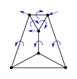
(b)

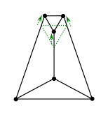
(c)

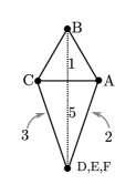
(d)

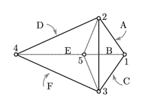
(e)

(f)

(g)

Figure 10: From a form diagram $(X,p)$ (a), a force diagram $(\tilde{X},q)$ (e) is drawn by holding the five interior edges of (a) in tension and the outside four in compression. We investigate the equivalent spaces to the mechanism (b) as described by Theorem 37. The motion of vertices, shifted by one quarter turn, are a parallel edge extension (c). The length changes of each member form the parallel realization (d). Over the dual, the mechanism (b) translates to a set of impossible edge rotations (f) by Theorem 34. These rotations in (f) are equivalent to a degree of self shear over the force diagram. Shifting these dual edge rotations by one quarter turn in the plane forms an axial self stress (g). By reciprocity and Theorem 33, (g) generates the parallel diagram (d).

4.3 The Polyhedral Lifting Correspondence

Dating back to Maxwell’s original papers [3, 4], self stresses over a loaded truss not only correspond to a dual force diagram, but also a “lifting” of cell structure to a polyhedron lying “above” the original truss in three dimensions. Because the base cell complex in planar graphic statics is spherical, the faces between the members of a loaded truss lift to a topologically spherical polyhedron [67]. See Figure 11 for an example of a lift over the self stressed cell complex of Figure 3. This lifting relation is commonly denoted the Maxwell–Cremona correspondence [68] and the lifted polyhedron itself has been shown to be a discrete Airy stress function over the underlying graph [60].

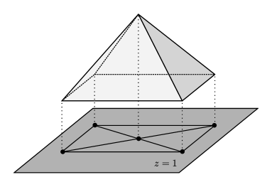
Figure 11: A lifting of the the cell complex in Figure 3 derived from the dimension of self stress.

A face lifted from $\mathbb{R}^{2}$ to $\mathbb{R}^{3}$ is modeled as the graph of an affine function over the face. Recall that an affine function on $\mathbb{R}^{n}$ with basis $\{x_{i}\}$ canonically takes the form $h(x_{1},\dots,x_{n})=\lambda_{1}x_{1}+\dots+\lambda_{n}x_{n}+\lambda_{n+1}$ for real parameters $\lambda_{i}$. The collection of these functions define the $n+1$ dimensional vector space $A\mathbb{R}^{n}$ of affine functions over $\mathbb{R}^{n}$. An equivalent perspective is that a affine function is a linear functional in $(\mathbb{R}^{n+1})^{\vee}$ evaluated on the hyperplane $H=\{x_{n+1}=1\}\subset\mathbb{R}^{n+1}$.

Lemma 38.

[67] There is an isomorphism $\eta:(\mathbb{R}^{n+1})^{\vee}\to A\mathbb{R}^{n}$ given by $\eta(h)=h|_{H}$, restriction of the function $h$ to the hyperplane $H$.

Here we let $X$ be realized in the hyperplane $H\subset\mathbb{R}^{3}$. Lifting $X$ from $H$ to a polyhedron in $\mathbb{R}^{3}$ requires lifting each face such that these glue together in the following sense. If $f$ and $g$ are neighboring faces incident to an edge $e$, then the graphs of two affine functions $h_{f}$ and $h_{g}$ over these faces must meet and be equal over the edge $e$. The difference $h_{f}-h_{g}$ will be the zero function restricted to the edge $e$, with gradient in $H$ perpendicular to $e$.

A collection of affine functions over faces $h=\{h_{f_{i}}\}$ is a lift of a diagram $(X,p)$ if and only if pairs of affine functions glue together over all conjoining edges. This is a cycle over the affine cosheaf $\mathcal{A}$ yet to be defined. The homology $H_{2}\mathcal{A}$ will consists of all polyhedral lifts of the underlying cell complex $X$.

In a polyhedral lift, not only faces but edges and vertices are lifted as well to $\mathbb{R}^{3}$. Modeling a lift of all cells, the cosheaf $\mathcal{A}$ has stalks comprised of spaces of locally defined affine functions, namely an isomorphism $\mathcal{A}_{c}\cong A\mathbb{R}^{\textrm{dim }c}$. To formalize this, let stalks $\mathcal{A}_{c}$ consist of equivalence classes of affine functions where $h_{c}\sim k_{c}$ if $h_{c}-k_{d}$ is the zero function when restricted to the cell $c$. Functions in the same equivalence class differ only away from their respective cell $c$. Under cosheaf extension maps $\mathcal{A}_{d\rhd c}$, equivalence classes merge as constraints from the underlying cell geometry becomes less restrictive. With stalks consisting of quotient vector spaces, the structure of $\mathcal{A}$ is of a quotient cosheaf.

Definition 39 (Zero Locus Cosheaf).

Suppose $(X,p)$ is a diagram in the hyperplane $H\subset\mathbb{R}^{n+1}$. Define $\mathcal{Z}$ as the zero locus cosheaf with stalks

$$\mathcal{Z}_{c}=\textrm{span}\{h\in A\mathbb{R}^{n}:h(p_{v})=0\textrm{ for every vertex }v\lhd c\}$$ (30)

of affine functions that are zero on the realization of $c$. Extension maps $\mathcal{Z}_{c\lhd d}$ are inclusions of subspaces $\mathcal{Z}_{d}\to\mathcal{Z}_{c}$.

The zero locus cosheaf $\mathcal{Z}$ has stalks of functions that vanish over their respective cells. Through the lens of Lemma 38, an affine function in $\mathcal{Z}_{c}$ is equivalent to a linear functional with the cell $c$ (in $H$) contained in its null space. It is best to require the vertex coordinates to have full dimensional span $\dim c+1$, otherwise the cell is degenerate. In dimension 2, specifying no degeneracy means no lifted faces are vertical with infinite gradient.

Definition 40 (Affine Cosheaf).

There is an injective map $\phi:\mathcal{Z}\to\overline{A\mathbb{R}^{n}}$ taking each subspace of affine functions $\mathcal{Z}_{c}$ into the total space of affine functions $\overline{A\mathbb{R}^{n}}_{c}$. Define the affine cosheaf $\mathcal{A}$ as the quotient of this inclusion map.

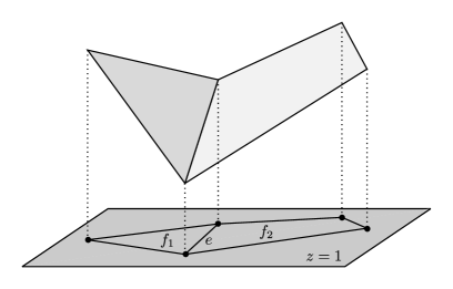
Figure 12: A local view of the affine cosheaf $\mathcal{A}$. There are two affine functions in $A\mathbb{R}^{2}$ restricted to the faces $f_{1}$ and $f_{2}$. The graphs of these functions are pictured. These functions coincide where they intersect over $e$.

The affine cosheaf $\mathcal{A}$ in dimension $n=2$ is most relevant to graphic statics. With the association $\mathcal{A}=\overline{A\mathbb{R}^{2}}/\mathcal{Z}$, elements of the stalks of $\mathcal{A}$ are equivalence classes, with each class consisting of functions that differ by an element of $\mathcal{Z}$. Because stalks $\mathcal{Z}_{f}$ are zero over non-degenerate faces, 2-chains of $\mathcal{A}$ are regular affine functions. A cycle $h\in H_{2}\mathcal{A}$ is a collection of these affine functions over faces where the difference of functions $h_{f}-h_{g}$ is in the zero class in $\mathcal{A}_{e}$, or an element of $\mathcal{Z}_{e}$, over every set $e\lhd f,g$. The piece-wise graph of the 2-cycle $a$ then is a polyhedron in $\mathbb{R}^{3}$ with lifted faces glued along their boundary edges. Elements of $H_{2}\mathcal{A}$ are polyhedral liftings of $(X,p)$.

Lemma 41.

The force cosheaf $\mathcal{F}$ over the hyperplane $H\subset\mathbb{R}^{3}$ and the cosheaf $\mathcal{Z}$ over $A\mathbb{R}^{2}$ are isomorphic.

Proof.

Here we define the cosheaf isomorphism $\tau:\mathcal{F}\to\mathcal{Z}$. Over an edge with incident vertices $u,v\lhd e$, the map $\tau_{e}$ is given by

$$\tau_{e}(w)=w(p_{u}\times p_{v})^{\vee}$$ (31)

where $\times$ is the cross product on vectors in $\mathbb{R}^{3}$ and $w\in\mathcal{F}_{e}\cong\mathbb{R}$ is a scalar representing a multiple of the vector $p_{u}-p_{v}$. We further define $\tau_{v}$ as

$$\tau_{v}(b)=(b\times p_{v})^{\vee}$$ (32)

over vertex $v$ where $b\in\mathcal{F}_{v}\cong\mathbb{R}^{2}\times\{1\}$ is a vector in $H\subset\mathbb{R}^{3}$. By counting dimensions of the resulting vector space of functions, $\tau$ is an isomorphism over each cell. Two calculations

$$\tau_{u}\circ\mathcal{F}_{e\rhd u}(w)=(w(p_{u}-p_{v})\times p_{u})^{\vee}=w(p_{u}\times p_{v})^{\vee}=\mathcal{Z}_{e\rhd u}\circ\tau_{e}(w)$$ (33)

$$\tau_{v}\circ\mathcal{F}_{e\rhd v}(w)=(w(p_{u}-p_{v})\times p_{v})^{\vee}=w(p_{u}\times p_{v})^{\vee}=\mathcal{Z}_{e\rhd v}\circ\tau_{e}(w)$$ (34)

prove that $\tau$ indeed is a cosheaf isomorphism. ∎

A corollary to Lemma 41 is the existence of a short exact sequence

$$0\to\mathcal{F}\xrightarrow{\phi\circ\tau}\overline{A\mathbb{R}^{2}}\to\mathcal{A}\to 0.$$ (35)

Note that for any edge with endpoints $v,u\lhd e$, for any two height values of $v$ and $u$ there exists an affine function $h_{e}$ over $e$ which takes these values over $v$ and $u$. Because there is always an edge connected to each vertex, the boundary map $\partial:C_{1}\mathcal{A}\to C_{0}\mathcal{A}$ is surjective and $H_{0}\mathcal{A}$ is trivial. Examining the resulting long exact sequence, we are greeted by a pair of short exact sequences.

$$0\to A\mathbb{R}^{2}\to H_{2}\mathcal{A}\to H_{1}\mathcal{F}\to 0$$ (36)

$$0\to H_{1}\mathcal{A}\to H_{0}\mathcal{F}\to A\mathbb{R}^{2}\to 0$$ (37)

Sequence (36) gives rise to the Maxwell–Cremona lifting correspondence.

Theorem 42 (The Maxwell–Cremona Correspondence [3, 69, 67]).

Let $(X,p)$ be spherical diagram in the projective plane $H\subset\mathbb{R}^{3}$. There is a bijection between self stresses $w\in H_{1}\mathcal{F}$ and polyhedral liftings $h\in H_{2}\mathcal{A}$ up to shifts of a global affine function. Over an edge bounded by two faces $e\lhd f,g$, the force $w_{e}$ over each edge is equal to

$$w_{e}=[e:f]\frac{h_{f}(p_{*})-h_{g}(p_{*})}{\det[p_{u},p_{v},p_{*}]}$$ (38)

where $\det$ is the determinant and $p_{*}$ is an arbitrary point in $H$ not collinear with $p_{u},p_{v}$. Expression (38) states that the difference in gradients between adjacent lifted faces is equal to the force within the connecting edge.

Proof.

The proof is similar to Theorem 33 and follows from the exact sequence (36). Any self stress $w\in H_{1}\mathcal{F}$ has a preimage $h\in H_{2}\mathcal{A}$ by exactness, and between any two preimages $h,k$ of $w$, the difference $h-k$ has the preimage of a global affine function in $A\mathbb{R}^{2}$. Cycles of $H_{2}\overline{A\mathbb{R}^{2}}\cong A\mathbb{R}^{2}$ are assignments of the same affine function to all cells. The polyhedral lifts $h,k$ differ by an affine function everywhere.

The value of edge forces $w_{e}$ follows from the definition of the connecting homomorphism $H_{2}\mathcal{A}\to H_{1}\mathcal{F}$. Applying the cosheaf boundary map $\partial_{\overline{A\mathbb{R}^{2}}}$ to the preimage of $h$ in $C_{2}\overline{A\mathbb{R}^{2}}$ results in an element $l\in C_{1}\overline{A\mathbb{R}^{2}}$ with terms $l_{e}=[e:f](h_{f}-h_{g})$ over each edge with incident cells $u,v\lhd e\lhd f,g$. Over such an edge, the affine function $h_{f}-h_{g}$ is zero on points $p_{u},p_{v}$ so $l$ is an element of $C_{1}\mathcal{Z}$.

Noting that each stalk $\mathcal{Z}_{e}$ is one dimensional spanned by the function $(p_{u}\times p_{v})^{\vee}$; it follows that the scalar $w_{e}$ satisfies $l_{e}=w_{e}(p_{u}\times p_{v})^{\vee}$. For an arbitrary choice of $p_{*}\in H$ not co-linear with $p_{u},p_{v}$, note that $(p_{u}\times p_{v})^{\vee}(p_{*})=\det[p_{u},p_{v},p_{*}]\neq 0$. Evaluating for $w_{e}$ we find

$$w_{e}=\frac{l_{e}(p_{*})}{\det[p_{u},p_{v},p_{*}]}=[e:f]\frac{h_{f}(p_{*})-h_{g}(p_{*})}{\det[p_{u},p_{v},p_{*}]}$$ (39)

is a constant scalar independent of $p_{*}$. Thus

$$l_{e}=[e:f]\frac{h_{f}(p_{*})-h_{g}(p_{*})}{\det[p_{u},p_{v},p_{*}]}(p_{u}\times p_{v})^{\vee}$$ (40)

over each edge. Finally, applying the cosheaf isomorphism $\tau^{-1}(l)=w$ results in the desired self-stress. ∎

The gradient of an affine function $h_{f}$ over the plane $H\subset\mathbb{R}^{3}$ consists of the first two coefficients only, the last being a constant term. These two coefficients can be considered as coordinates of the dual vertex $\tilde{f}$ in $H$. These coordinates assemble into a perpendicular reciprocal diagram. This outlines an alternative way of generating dual figures; starting from the space of polyhedral lifts of $(X,p)$ there is an injective map to the space of perpendicular reciprocal diagrams $(\tilde{X},q)$ over any cellular oriented manifold [15].

4.4 Boundary Conditions

In prior discussions, a truss is modeled by a cell complex $X$ with the specific topology of the sphere $S^{2}$. Because a sphere has empty boundary it was not possible to model boundary forces that may be imparted on the truss. These boundary conditions consist of external or reaction loads imparted onto the structure. With the vast majority of trusses in practice are subject to external loads, an alternative cellular topology must be selected.

External loads acting on a truss are modeled by edges $e_{*}$ connected to the truss only at one end $v\lhd e_{*}$ along the exterior of the truss. Here $v$ is the point of application of the foreign force, applied along the line of action of $e_{*}$. These edges may be external loads $e_{l}$ or reaction forces $e_{r}$; both are treated equally as partially open ended edges. With this, the truss including these open ended edges $X$ has the topology of an open disk $B^{2}\subset S^{2}$.

Considering boundary conditions, the homology $H_{1}\mathcal{F}$ of the force cosheaf still describes the space of canceling edge forces. These include self stresses as well as equilibrium stresses induced by boundary loads. If the values of external loads $e_{l}$ are provided beforehand, solving for internal and reaction forces is equivalent to finding a cycle in $H_{1}\mathcal{F}$ with the specified values over edges $e_{l}$.

Graphic statics readily generalizes to the setting of boundary conditions. The most important difference is that the open disk $B^{2}$ has (Borel-Moore) homology $H_{2}B^{2}\cong\mathbb{R}$, $H_{1}B^{2}=0$ and $H_{0}B^{2}=0$. The key difference to spherical topology is that $H_{0}$ of $X$ (and $H_{0}$ of constant cosheaves $\overline{\mathbb{R}^{n}}$) vanish.

Algebraic relations in graphic statics earlier in Section 4.1 were found to be governed by the two exact sequences (25) and (26). When $X$ takes the topology of the open disk, the former sequence remains the same while the latter takes the form

$$0\to H_{1}\mathcal{G}\to H_{0}\mathcal{F}\to 0.$$ (41)

In other words, the space of degrees of freedom $H_{0}\mathcal{F}$ is isomorphic to dual edge rotations $H^{1}\tilde{\mathcal{G}}$ without needing to account for the global translations. External edges $e_{l}$ and $e_{r}$ may lock the truss $(X,p)$ in place, so free translations may not exist at all. Apart from this consideration of global translation, Theorems 33 and 34 remain valid in the presence of boundary conditions.

In the setting of plane reciprocity the form diagram and the force diagram are no longer symmetrically dual. When $X$ has the topology of an open disk, its dual $\tilde{X}$ has the dissimilar topology of a closed disk. This is Lefschetz duality over subsets of manifolds, here $S^{2}$. If $(X,p)$ is an open form diagram with boundary conditions and $(\tilde{X},q)$ is a closed force diagram, this topological change eliminates the need to reduce by the translation factor of $\mathbb{R}^{2}$ in points (i) and (ii) in Theorem 37.

For the polyhedral lifting correspondence, Theorem 42 is unchanged over a truss with boundary conditions, as Sequence 36 does not consider zero dimensional homology. In effect, polyhedral lifts can follow from equilibrium loading conditions as well.

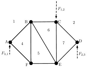
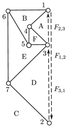
Figure 13: A truss with boundary conditions $X$ with one dimension of stress is pictured (left). There is one dimension of non-trivial realization of the dual $\tilde{X}$ (right).

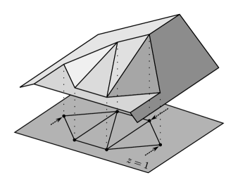
Figure 14: A lifting of the truss with boundary conditions in Figure 13.

5 Beyond Planar Graphic Statics

There is the natural question of how to extend graphic statics to non-spherical topology, allowing for dual diagrams from non-planar trusses. Previous approaches have focused on dualizing the underlying graph, not the full oriented manifold $M_{g}$ of genus $g$ as we will here [19, 20].

Theorem 43 (Higher Genus Plane Graphic Statics).

Let $(X,p)$ be a diagram with the topology of an oriented surface $M_{g}$ realized in $\mathbb{R}^{2}$. If the dimension of axial self stress $\dim H_{1}\mathcal{F}$ is greater than $4g$, then there exists a non-trivial parallel dual realization $q$ of $\tilde{X}$ in $\mathbb{R}^{n}$

Proof.

For $\mathcal{F}$ in ambient dimension $n$, the long exact sequence for the filtration $\mathcal{F}\to\overline{\mathbb{R}^{2}}$ is

$$0\to\mathbb{R}^{2}\to H_{2}\overline{\mathbb{R}^{2}}/\mathcal{F}\xrightarrow{\vartheta}H_{1}\mathcal{F}\xrightarrow{\phi}H_{1}\overline{\mathbb{R}^{2}}\to\dots$$ (42)

Since $\dim H_{1}M_{g}=2g$, it follows that $H_{1}\overline{\mathbb{R}^{2}}\cong\mathbb{R}^{4g}$. Thus under the assumptions the map $\phi$ above cannot be injective. By exactness of sequence (42), the connecting homomorphism $\vartheta$ is not the zero map. Any non-trivial preimage by $\vartheta$ correlates to a non-trivial parallel realization of $\tilde{X}$. ∎

We take care to note that the resulting realizations of $\tilde{X}$ are not the algebraic duals in graph theory, where simple cycles are dual to minimal cuts. Hence, the above theorem does not contradict Whitney’s duality [70], which states that a graph has a dual if and only if it is planar. Instead, Theorem 43 is a statement strictly about geometric duals, linking vertices to dual faces, edges to dual edges, and faces to dual vertices.

Another point is that a realization of the torus $M_{1}$ is a mapping to $\mathbb{R}^{2}$ and is not a periodic tiling of the plane, as is the case in [71, 68].

Example 44 (Dependence on Graph Embedding).

Finding dual realizations from a non-planar graph depends on its embedding in an oriented surface $M_{g}$. The particular introduction of face cells determines what dual realizations result from a self-stress. Even for planar graphs embedded in the sphere $S^{2}$, the choice of realization does not necessarily determine the dual graph (unless the graph is 3-connected [72]).

To demonstrate, let $(X,p)$ be the cellular decomposition of the torus $M_{1}$ pictured in Figure 15(a) where it contains the complete bipartite graph $K_{3,3}$ as a subgraph. The realization of $X$ in $\mathbb{R}^{2}$ pictured in (b) has a non-planar 1-skeleton and four dimensions of self stress in $H_{1}\mathcal{F}_{X}$. There is one nontrivial dimension of dual realizations of $\tilde{X}$, pictured in (c). The 1-skeleton of $\tilde{X}$ is planar, but there is no way to embed faces of $\tilde{X}$ in $\mathbb{R}^{2}$ without overlapping.

This process outlines a canonical way to dualize a cell complex realized in $\mathbb{R}^{2}$, but not a canonical way to dualize the underlying graphs. The cell complex $X^{\prime}$ in (d) has a homeomorphic 1-skeleton to (a), but with $(X^{\prime},p)$ utilizing the same realization (b), the space $H^{0}\tilde{\mathcal{G}}_{\tilde{X}^{\prime}}$ and all dual realizations of $\tilde{X}^{\prime}$ are trivial.

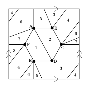
(a) Topology of a cellular decomposition $X$ of $M_{1}$ containing $K_{3,3}$, a non-planar graph.

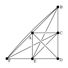
(b) A realization of $X$ in the plane.

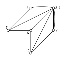
(c) A realization of a dual diagram $\tilde{X}$ to that in (b).

(d) An alternate cellular decomposition $X^{\prime}$ of $M_{1}$ with the same 1-skeleton as (a).

Figure 15: Graphic Statics duality with non-planar graphs

There is an analogue to Theorem 43 for polyhedral lifts over higher genus manifolds.

Theorem 45 (Higher Genus Polyhedral Lifting).

Let $(X,p)$ be a cellular decomposition of an oriented surface $M_{g}$ realized in $\mathbb{R}^{2}$. If the dimension of the space of self stresses $H_{1}\mathcal{F}$ is greater than $6g$, then there exists a self stress of $X$ and a non-trivial polyhedral lifting to $\mathbb{R}^{3}$, where the difference in gradient between adjacent lifted faces is equal to the force within the connecting edge.

Proof.

Recall that the space of affine functions $A\mathbb{R}^{2}$ is three dimensional. Since $\dim H_{1}M_{g}=2g$, it follows that $H_{1}\overline{A\mathbb{R}^{2}}\cong\mathbb{R}^{6g}$. If $H_{1}\mathcal{F}$ has dimension greater than $6g$, the map $\phi:H_{1}\mathcal{F}\to H_{1}\overline{A\mathbb{R}^{2}}$ cannot be injective. By exactness of sequence (42), the connecting homomorphism $\vartheta$ cannot be the zero map. Any non-trivial preimage by $\vartheta$ correlates to a non-trivial polyhedral lift. ∎

A triangulated surface in general position has non-trivial polyhedral lifts. In a triangular mesh every node is incident to only triangular faces, and a lift of the node lifts these triangles into a cone. Consequently, a regular cellular decomposition of a manifold into triangles results in a $|V|$ dimensional space of polyhedral lifts, where $|V|$ is the number of vertices.

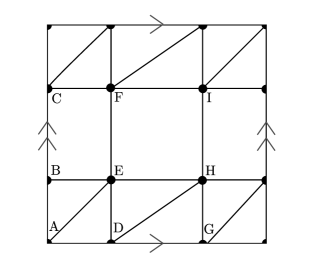
(a) A cell complex $X$ with topology $M_{1}$.

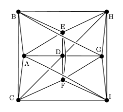
(b) A form diagram $(X,p)$ in the plane with 9 degrees of self stress.

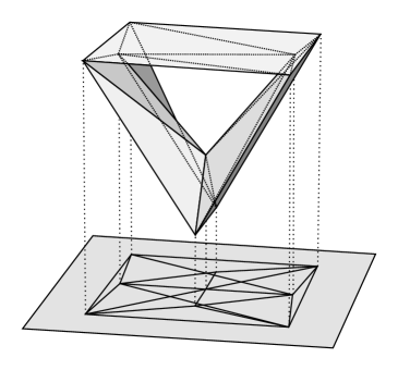
(c) A polyhedral lift of $X$ to $\mathbb{R}^{3}$.

Figure 16: A cell complex $X$ with topology (a) is realized in (b). The truss is rigid and by the Euler characteristic (10), we observe that there are $H_{1}\mathcal{F}=24-18+3=9$ degrees of self stress. With $9>6$, Theorem 45 applies and there is at least one non-trivial dimension of torus polyhedral lifting in $H_{2}\mathcal{A}/\overline{A\mathbb{R}^{2}}$, with a representative pictured in (c). Numerical computations indicates that there are in fact four dimensions of lifts up to shifts by global affine functions.

In planar graphic statics, Theorems 33 and 42 prove that a structure has an non-trivial reciprocal diagram if and only if the structure has a non-trivial polyhedral lifting. Over a torus and higher genus surfaces, this relationship no longer holds true [15]. Polyhedral lifts guarantee reciprocal figures but the converse does not hold; Figure 17 portrays a counterexample.

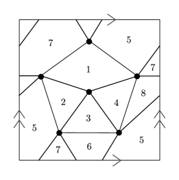
(a) Toroidal topology of $X$.

(b) A form diagram $(X,p)$ with 5 degrees of self stress.

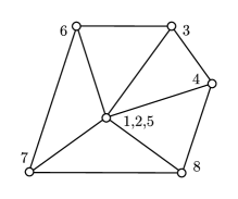
(c) A dual force diagram is generated.

Figure 17: An example of a toroidal figure with reciprocal diagram but no non-trivial polyhedral lift. In the form diagram (b), faces 5 and 1 lock all vertices in a single plane preventing lifts. There are 5 degrees of self stress, meaning a non-trivial force diagram exists by Theorem 43 in (c).

Figure 18: A polyhedral lift of a cell complex with the topology of a two holed torus $M_{2}$ is pictured. Numerical computation shows this particular realization has 8 degrees of self stress, which is less than the 13 degree requirement to guarantee the existence of a lift. Due to the specific geometry of the realization there are 3 dimensions of polyhedral lifts up to shift by affine function. One dimension determines width of the bounding box, the other two determine the vertical position of the rectangular voids.

6 Conclusion

We proposed a development of algebraic graphic statics following sheaf and cosheaf constructions. These formal methods from algebraic topology allow for extensions to high genus surfaces. We precisely defined reciprocal diagrams in the plane and found $H_{1}$ of the base surface to obstruct their formation. These homological constraints impede the formation of lifts or dual diagrams in the plane. There are numerous future avenues of research.

6.1 Sheaf Finite Elements

The finite element method is central to modern structural analysis, fluid flow, and heat transfer mathematical modeling. In summary, a complex domain $M$ is subdivided and discretized into a finite number of geometrically simple elements [73]. A solution to a Poisson problem with boundary conditions over $M$ is approximated by algebraic approximation functions between the finite elements, these derived from weighted integrals over local neighborhoods. These approximation functions are typically polynomials and the entire discrete system is otherwise known as a spline [55]. Introduced approximation errors introduced can be bounded and shown (in a well formulated model) to converge to 0 as the mesh is refined.

It has been shown that polynomial splines are homological and can be described by cosheaves [31]. In this setting the force cosheaf $\mathcal{F}$ is a spline of constant functions and the affine cosheaf $\mathcal{A}$ is a spline of linear-affine functions. The stiffness matrix problem $a=\Delta_{\mathcal{F}}b$ and its pseudo-inverse are quintessential in linear-elastic mechanics. There is potential to extend these homological methods to other finite element processes.

6.2 Trusses on Manifolds

Definition 16 of the force cosheaf suggests an extension of truss mechanics to general manifolds. Instead of a cell complex $X$ being realized in Euclidean space, we realize vertices $v$ with positions $p_{v}\in M$ and where edges are geodesics $\gamma_{e}:\mathbb{R}^{1}\to M$ (one must take care that these geodesics exist e.g. by the Hopf–Rinow theorem). To an edge $u,v\lhd e$, the force cosheaf $\mathcal{F}$ would have extension maps $\mathcal{F}_{e\rhd u}$ and $\mathcal{F}_{e\rhd v}$ the push-forward $(\gamma_{e})_{*}$ mapping to $T_{p_{u}}M$ and $T_{p_{v}}M$ along the curve. A more complete analysis of manifold trusses warrants further attention.

6.3 3D Graphic Statics

The homological constructions here are sufficient to generalize to higher dimensions. In 3D vector graphic statics the form diagram is embedded in $\mathbb{R}^{3}$. In Section 4.1 we can replace all occurrences of $\mathbb{R}^{2}$ with $\mathbb{R}^{3}$, leading to 3D vector graphic statics duality. Both Theorems 33 and Theorems 34 can be translated. As the technique of rotating stalks by one quarter turn does not transfer there is no notion of reciprocity.

Another avenue is in 3D polyhedral graphic statics which has shown to have geometric relations far more complex than the 2D setting [2]. Investigations show that the linear algebraic relations when including 3-cells are described by a spectral sequence of pertinent cosheaves.

References

- [1] P. Varignon, Nouvelle Mecanique Ou Statique: Dont Le Projet Fut Donné En MDCLXXXVII. chez Claude Jombert, 1725.
- [2] M. Akbarzadeh, “3D Graphical Statics Using Reciprocal Polyhedral Diagrams,” Ph.D. dissertation, 2016.
- [3] J. C. Maxwell, “XLV. On reciprocal figures and diagrams of forces,” The London, Edinburgh, and Dublin Philosophical Magazine and Journal of Science, vol. 27, no. 182, pp. 250–261, 1864.
- [4] ——, “I.—On Reciprocal Figures, Frames, and Diagrams of Forces,” Transactions of the Royal Society of Edinburgh, vol. 26, no. 1, pp. 1–40, 1870.
- [5] L. Cremona, Le Figure Reciproche Nella Statica Grafica. Tipografia di G. Bernardoni, 1872.
- [6] ——, Graphical Statics: Two Treatsies on the Graphical Calculus and Reciprocol Figures in Graphical Statics, 1890.
- [7] W. J. M. Rankine, “XVII. Principle of the equilibrium of polyhedral frames,” The London, Edinburgh, and Dublin Philosophical Magazine and Journal of Science, vol. 27, no. 180, pp. 92–92, 1864.
- [8] B. Rasch and F. Otto, “Finding Form,” 1996.
- [9] L. Fuhrimann, V. Moosavi, P. O. Ohlbrock, and P. D’acunto, “Data-driven design: Exploring new structural forms using machine learning and graphic statics,” in Proceedings of IASS Annual Symposia, vol. 2018. International Association for Shell and Spatial Structures (IASS), 2018, pp. 1–8.
- [10] M. Akbarzadeh, T. Van Mele, and P. Block, “Three-dimensional graphic statics: Initial explorations with polyhedral form and force diagrams,” International Journal of Space Structures, vol. 31, no. 2-4, pp. 217–226, 2016.
- [11] L. L. Beghini, J. Carrion, A. Beghini, A. Mazurek, and W. F. Baker, “Structural optimization using graphic statics,” Structural and Multidisciplinary optimization, vol. 49, no. 3, pp. 351–366, 2014.
- [12] M. Konstantatou and A. Mcrobie, “Graphic statics for optimal trusses & Geometry-based structural optimisation,” no. June, 2018.
- [13] E. Saliklis, Structures: A Geometric Approach. Springer, 2019.
- [14] H. Crapo, “Structural Rigidity,” Structural Topology Vol.1, vol. 1, pp. 26–45, 1979.
- [15] H. Crapo and W. Whiteley, “Plane self stresses and projected polyhedra I : The Basic Pattern,” Structural Topology, vol. 20, 1993.
- [16] C. R. Calladine, “Buckminster Fuller’s ”Tensegrity” structures and Clerk Maxwell’s rules for the construction of stiff frames,” International Journal of Solids and Structures, vol. 14, no. 2, pp. 161–172, 1978.
- [17] S. Pellegrino, “Mechanics of kinematically indeterminate structures,” Ph.D. dissertation, University of Cambridge, Cambridge.
- [18] T. Tachi, “Design of Infinitesimally and Finitely Flexible Origami Based on Reciprocal Figures,” Journal for Geometry and Graphics, vol. 16, no. 2, pp. 223–234.
- [19] A. Micheletti, “On generalized reciprocal diagrams for self-stressed frameworks,” International Journal of Space Structures, vol. 23, no. 3, pp. 153–166, 2008.
- [20] T. Van Mele and P. Block, “Algebraic graph statics,” CAD Computer Aided Design, vol. 53, pp. 104–116, 2014.
- [21] A. McRobie, W. Baker, T. Mitchell, and M. Konstantatou, “Mechanisms and states of self-stress of planar trusses using graphic statics, part II: Applications and extensions,” International Journal of Space Structures, vol. 31, no. 2-4, pp. 102–111, 2016.
- [22] A. McRobie, M. Konstantatou, G. Athanasopoulos, and L. Hannigan, “Graphic kinematics, visual virtual work and elastographics,” Royal Society Open Science, vol. 4, no. 5, 2017.
- [23] M. Akbarzadeh, M. Mahnia, R. Taherian, and A. H. Tabrizi, “Prefab, Concrete polyhedral frame: Materializing 3D graphic statics,” in Proceedings of IASS Annual Symposia, vol. 2017. International Association for Shell and Spatial Structures (IASS), 2017, pp. 1–10.
- [24] M. Bolhassani, M. Akbarzadeh, M. Mahnia, and R. Taherian, “On structural behavior of a funicular concrete polyhedral frame designed by 3D graphic statics,” in Structures, vol. 14. Elsevier, 2018, pp. 56–68.
- [25] M. Akbarzadeh, M. Bolhassani, A. Nejur, J. R. Yost, C. Byrnes, J. Schneider, U. Knaack, and C. B. Costanzi, “The design of an ultra-transparent funicular glass structure,” in Structures Congress 2019: Blast, Impact Loading, and Research and Education. American Society of Civil Engineers Reston, VA, 2019, pp. 405–413.
- [26] M. Hablicsek, M. Akbarzadeh, and Y. Guo, “Algebraic 3D graphic statics: Reciprocal constructions,” CAD Computer Aided Design, vol. 108, pp. 30–41, 2019.
- [27] A. McRobie, “The geometry of structural equilibrium,” Royal Society Open Science, vol. 4, no. 3, 2017.
- [28] M. Konstantatou, P. D’Acunto, and A. McRobie, “Polarities in structural analysis and design: N-dimensional graphic statics and structural transformations,” International Journal of Solids and Structures, vol. 152–153, pp. 272–293, 2018.
- [29] A. McRobie, “Maxwell and Rankine reciprocal diagrams via Minkowski sums for two-dimensional and three-dimensional trusses under load,” International Journal of Space Structures, vol. 31, no. 2-4, pp. 203–216, Jun. 2016.
- [30] A. McRobie, C. Millar, and W. F. Baker, “Stability of trusses by graphic statics,” Royal Society Open Science, vol. 8, no. 6, p. 201970, 2021.
- [31] R. Ghrist, Elementary Applied Topology Ed 1.0. Createspace, 2014.
- [32] G. E. Bredon, Sheaf Theory. Springer New York, 1997.
- [33] S. Mac Lane and I. Moerdijk, Sheaves in Geometry and Logic. Springer, 1994.
- [34] A. D. Shepard, “A Cellular Description of the Derived Category of a Stratified Space,” 1986.
- [35] J. Curry, “Sheaves, Cosheaves and Applications,” Ph.D. dissertation, University of Pennsylvania, Mar. 2013.
- [36] R. Ghrist and Y. Hiraoka, “Network codings and sheaf cohomology,” IEICE Proceedings Series, vol. 45, no. A4L-C3, 2011.
- [37] V. De Silva, E. Munch, and A. Patel, “Categorified reeb graphs,” Discrete & Computational Geometry, vol. 55, no. 4, pp. 854–906, 2016.
- [38] M. Robinson, “Asynchronous logic circuits and sheaf obstructions,” Electronic Notes in Theoretical Computer Science, vol. 283, pp. 159–177, 2012.
- [39] R. Ghrist and S. Krishnan, “Positive Alexander duality for pursuit and evasion,” 2017.
- [40] H. R. Yoon, “Cellular sheaves and cosheaves for distributed topological data analysis,” Ph.D. dissertation, University of Pennsylvania, 2018.
- [41] H. R. Yoon and R. Ghrist, “Persistence by parts: Multiscale feature detection via distributed persistent homology,” arXiv preprint arXiv:2001.01623, 2020.
- [42] F. Russold, “Persistent sheaf cohomology,” arXiv preprint arXiv:2204.13446, 2022.
- [43] J. Hansen and R. Ghrist, “Distributed optimization with sheaf homological constraints,” in 2019 57th Annual Allerton Conference on Communication, Control, and Computing (Allerton). IEEE, 2019, pp. 565–571.
- [44] J. Hansen and T. Gebhart, “Sheaf neural networks,” arXiv preprint arXiv:2012.06333, 2020.
- [45] C. Bodnar, F. Di Giovanni, B. Chamberlain, P. Liò, and M. Bronstein, “Neural sheaf diffusion: A topological perspective on heterophily and oversmoothing in gnns,” Advances in Neural Information Processing Systems, vol. 35, pp. 18 527–18 541, 2022.
- [46] F. Barbero, C. Bodnar, H. S. d. O. Borde, M. Bronstein, P. Veličković, and P. Liò, “Sheaf Neural Networks with Connection Laplacians,” arXiv preprint arXiv:2206.08702, 2022.
- [47] J. Hansen and R. Ghrist, “Toward a spectral theory of cellular sheaves,” Journal of Applied and Computational Topology, vol. 3, no. 4, pp. 315–358, 2019.
- [48] ——, “Opinion dynamics on discourse sheaves,” SIAM Journal on Applied Mathematics, vol. 81, no. 5, pp. 2033–2060, 2021.
- [49] R. Ghrist, “Network SheafModels for social information dynamics,” in 2022 IEEE 8th International Conference on Collaboration and Internet Computing (CIC). IEEE, 2022, pp. 31–37.
- [50] R. Ghrist and H. Riess, “Cellular Sheaves of Lattices and the Tarski Laplacian,” Homology, Homotopy, and Applications 24(1).
- [51] H. Riess and R. Ghrist, “Diffusion of Information on Networked Lattices by Gossip,” arXiv e-prints, pp. arXiv–2204, 2022.
- [52] Z. Cooperband and R. Ghrist, “Towards Homological Methods In Graphic Statics,” Proceedings of the IASS 2023.
- [53] OY. Viro, “Some integral calculus based on Euler characteristic,” Lecture Notes in Mathematics, pp. 127–138, 1988.
- [54] P. Schapira, “Tomography of constructible functions,” in International Symposium on Applied Algebra, Algebraic Algorithms, and Error-Correcting Codes. Springer, 1995, pp. 427–435.
- [55] L. J. Billera, “Homology of smooth splines: Generic triangulations and a conjecture of Strang,” Transactions of the american Mathematical Society, vol. 310, no. 1, pp. 325–340, 1988.
- [56] S. Yuzvinsky, “Modules of splines on polyhedral complexes,” Mathematische Zeitschrift, vol. 210, pp. 245–254, 1992.
- [57] H. Crapo, “Applications of geometric homology,” in French Workshop on Geometry and Robotics. Springer, 1988, pp. 213–224.
- [58] ——, “Projective configurations: Their invariants and homology,” in Proceedings of the Royal Irish Academy. Section A: Mathematical and Physical Sciences, no. P.109. Royal Irish Academy, 1995, pp. 1–24.
- [59] W. Whiteley, “An Analogy in Geometric Homology: Rigidity and Cofactors on Geometric Graphs,” Mathematical Essays in honor of Gian-Carlo Rota, no. January 1998, 1998.
- [60] T. Mitchell, W. Baker, A. McRobie, and A. Mazurek, “Mechanisms and states of self-stress of planar trusses using graphic statics, part I: The fundamental theorem of linear algebra and the Airy stress function,” International Journal of Space Structures, vol. 31, no. 2-4, pp. 85–101, 2016.
- [61] C. Williams and A. McRobie, “Graphic statics using discontinuous Airy stress functions,” International Journal of Space Structures, vol. 31, no. 2-4, pp. 121–134, 2016.
- [62] H. Crapo and W. Whiteley, “Statics of Frameworks and Motions of Panel Structures, a Projective Geometric Introduction,” Structural Topology, vol. 6, 1982.
- [63] W. Whiteley, “Realizability of polyhedra,” Structural Topology, no. January 1979, pp. 46–58, 1979.
- [64] J. Hansen, “Laplacians of Cellular Sheaves: Theory and Applications,” Ph.D. dissertation, University of Pennsylvania, 2020.
- [65] A. Hatcher, Algebraic Topology. Cambridge University Press, 2002.
- [66] R. Connelly and S. D. Guest, Frameworks, Tensegrities and Symmetry: Understanding Stable Structures. Cornell Cornell University, College of Arts and Sciences, 2015, 2015.
- [67] J. E. Hopcroft and P. J. Kahn, “A paradigm for robust geometric algorithms,” Algorithmica, vol. 7, no. 1-6, pp. 339–380, 1992.
- [68] J. Erickson and P. Lin, “A Toroidal Maxwell-Cremona-Delaunay Correspondence,” 2020.
- [69] W. Whiteley, “Motions and Stresses of Projected Polyhedra,” Structural Topology, vol. 7, no. June, pp. 13–38, 1982.
- [70] H. Whitney, “Non-Separable and Planar Graphs,” Proceedings of the National Academy of Sciences of the United States of America, vol. 17, no. 2, pp. 125–127, 1931.
- [71] C. Borcea and I. Streinu, “Liftings and stresses for planar periodic frameworks,” Discrete & computational geometry, vol. 53, no. 4, pp. 747–782, 2015.
- [72] H. Whitney, “A Set of Topological Invariants for Graphs,” American Journal of Mathematics, vol. 55, no. 1, pp. 231–235, 1933.
- [73] J. N. Reddy, Introduction to the Finite Element Method. McGraw-Hill Education, 2019.