Synthetic X-ray emission from white dwarf accreting planetary material

Abstract

The emission of hard X-rays associated with white dwarfs (WD) can be generated by the presence of a stellar companion either by the companion’s coronal emission or by an accretion disk formed by material stripped from the companion. Recent studies have suggested that a Jupiter-like planet can also be donor of material whose accretion onto the WD can generate hard X-rays. We use the guacho code to reproduce the conditions of this WD-planet scenario. With the example of the hard X-ray WD KPD 0005+5106, we explore different terminal wind velocities and mass-loss rates of a donor planet for a future network of simulations to investigate the luminosity and the spectral and temporal properties of the hard X-ray emission in WD-planet systems. Our simulations show that the material stripped from the planet forms a disk and accretes onto the WD to reach temperatures high enough to generate hard X-rays as usually seen in X-ray binaries with low-mass companions. For high terminal wind velocities, the planet material does not form a disk, but it rather accretes directly onto the WD surface. The simulations reproduce the X-ray luminosity of another X-ray accreting WD (G 29$-$38), and only for some times reaches the hard X-ray luminosity of KPD 0005+5106. The X-ray variability is stochastic and does not reproduce the period of KPD 0005+5106, suggesting that additional physical processes (e.g., hot spots resulting from magnetic channelling of the accreting material) need to be explored.

1 Introduction

White dwarfs (WDs) represent the final stage of the evolution of low- and intermediate-mass stars (1 M${}_{\odot}\lesssim M_{\mathrm{i}}\lesssim 8$ M_⊙). These stars lose most of their initial mass through a dense and slow wind ($\dot{M}\lesssim$10^-4 M_⊙ yr^-1, $v\approx 10$ km s^-1; see Scicluna et al., 2022, and references therein) when evolving through the asymptotic giant branch (AGB) phase. Having exposed their cores, they become hot enough to develop fast winds ($v_{\infty}\gtrsim$10³ km s^-1; Guerrero & De Marco, 2013) and strong UV photon fluxes. The combinations of these effects create what we know as planetary nebulae (PNe; Kwok, 2000) whose final fate is to expand and mix into the interstellar medium (ISM) whilst the progenitor star evolves along the WD cooling track.

As stars evolve, their planetary systems co-evolve. In particular the extreme variation of the stellar and wind parameters during the evolution of Solar-like stars will create harsh environments that may endanger the survival of planetary systems. It has been proposed that planets located $\lesssim$1 AU from their host stars (e.g., Mercury or Venus) will be evaporated during the main sequence phase (Rao et al., 2021) or engulfed during the inflation of the stellar outer layers during the AGB phase (Privitera et al., 2016). Those located farther away will spiral in or migrate out as a result of the reduction of the gravitational potential of the star. In addition, any remaining planet could be photoevaporated by the UV flux during the post-AGB phase (Villaver & Livio, 2007). Against all odds, planets and planetary material have been discovered orbiting WD stars (see, e.g., Veras, 2021).

For decades, the IR excess observed from WDs (see, e.g., Zuckerman & Becklin, 1987; Hansen et al., 2006; Bilíková et al., 2012; Xu et al., 2020) and the presence of metals in the atmospheres of cool degenerate DZ WDs (see, e.g., Jura, 2003, 2008; Farihi et al., 2010) have been suggested to be a signature of the presence of planets or the remains of planetary systems. After the discovery of a Jupiter-like planet around WD 1856+534 (Vanderburg et al., 2020; Alonso et al., 2021), several works have addressed the search and discovery of planets, planetary material and other sub-stellar objects around WDs (see, e.g., Blackman et al., 2021; Brandner et al., 2021; Fitzmaurice et al., 2023; Martin et al., 2021; Van Grootel et al., 2021; van Roestel et al., 2021; Kosakowski et al., 2022; Walters et al., 2022).

Recently, X-ray observations have been used to suggest the presence of planets or planetary material around WDs. Chu et al. (2021) presented the analysis of X-ray emission associated with putative single hot ($T_{\mathrm{eff}}>10^{5}$ K) WDs. They used Chandra and XMM-Newton observations of KPD 0005+5106 to unveil variability in the hard X-ray band (0.6–3.0 keV) with a period of 4.7$\pm$0.3 hr in the WD. In general, hard X-ray emission from WDs is produced by either a companion’s coronal activity or the acretion of a companion’s material onto a WD (see O’Dwyer et al., 2003; Chu et al., 2004a; Bilíková et al., 2010). However, using H$\alpha$ and multi-instrument IR observations of KPD 0005+5106, Chu et al. (2021) were able to reject any stellar companion as late as M 8V. Assuming that the periodicity of the hard X-ray emission detected from KPD 0005+5106 is the orbital period of a sub-stellar companion (a M9V star, a T-type brown dwarf and a Jupiter-like planet), Chu et al. (2021) estimated that only a Jupiter-like planet would be able to fill its Roche Lobe to transfer material to the WD. Using the hard X-ray luminosity of KDP 0005+5106 ($L_{\mathrm{X,hard}}=3\times 10^{30}$ erg s^-1) they estimated an instantaneous accretion rate of $\dot{M}_{\mathrm{ac}}$=$1.45\times 10^{14}$ g s^-1(=$2.3\times 10^{-12}$ M_⊙ yr^-1).

More recently Cunningham et al. (2022) used Chandra observations of the WD G 29–38 to report the detection of X-ray emission. G 29-38 is a widely studied metal-polluted WD of spectral type DAZ (Koester et al., 1997), which has been known to exhibit IR excess (Zuckerman & Becklin, 1987; Graham et al., 1990) that has been attributed to the accretion from a dust-rich disk (Jura, 2003). Cunningham et al. (2022) suggested that the X-ray emission is produced by accretion of the planetary material onto G 29-38. Our recent analysis of archival XMM-Newton observations of G 29-38 (Estrada-Dorado et al., 2023) confirmed the X-ray emission from G 29-38, with an X-ray luminosity in the 0.3–7.0 keV energy band of $L_{\mathrm{X}}=(8.3\pm 4.1)\times 10^{25}$ erg s^-1, which implies an accretion rate of $\dot{M}_{\mathrm{ac}}=4.01\times 10^{9}$ g s^-1(=6.45$\times 10^{-17}$ M_⊙ yr^-1).

In this paper we present a set of radiation-hydrodynamic simulations of mass-losing planets orbiting a WD to study the production of X-ray emission. The physical properties of the circumstellar material derived from our simulations are post-processed using the Chianti database (Del Zanna et al., 2021) to derive X-ray properties. We discuss our results in the light of previous observations of putatively single WDs with X-ray emission such as the metal-polluted WD G 29$-$38 and the hard X-ray-emitting WD KPD 0005+5106.

This paper is organized as follows. In Section 2 we describe the code and initial conditions of the simulations. In Section 3 we present our numerical results and the creation of synthetic X-ray properties and our discussion is presented in Section 4. Finally, a summary of the work is presented in Section 5.

2 Numerical simulations

2.1 The guacho code

We use the well-tested radiation-hydrodinamic 3D code guacho (Esquivel et al., 2009; Esquivel & Raga, 2013) to model the interaction of a mass-losing Jupiter-like planet around a WD. guacho includes a modified version of the ionizing radiation transfer presented by Raga et al. (2009). It solves the gas-dynamic equations with a second order accurate Godunov-type method using a linear slope-limited reconstruction and the Harten-Lax-van Leer-Contact (HLLC) approximate Riemann solver (Toro et al., 1994) implemented on a uniform Cartesian grid.

Simultaneously with the Euler equations, the code solves the rate equation for neutral and ionized hydrogen

$$\frac{\partial n_{\mathrm{HI}}}{\partial t}+\nabla\cdot(n_{\mathrm{HI}}\textbf{u})=n_{\mathrm{e}}n_{\mathrm{HII}}\alpha(T)-n_{\mathrm{HI}}n_{\mathrm{HII}}C(T)-n_{\mathrm{HI}}\phi,$$ (1)

where u is the flow velocity, $n_{\mathrm{e}}$, $n_{\mathrm{HI}}$ and $n_{\mathrm{HII}}$ are the electron, neutral hydrogen and ionized hydrogen number densities, respectively, $\alpha(T)$ is the recombination coefficient, $C(T)$ is the collisional ionization coefficient, and $\phi$ is the H photoionization rate due to a central source. The photoionizing rate is computed with the Monte-Carlo ray tracing method described by Esquivel & Raga (2013) and Schneiter et al. (2016).

The ionization fraction is defined as:

$$\chi=\frac{n_{\mathrm{HII}}}{n_{\mathrm{HI}}+n_{\mathrm{HII}}},$$ (2)

with the total density defined as $n_{\mathrm{HI}}+n_{\mathrm{HII}}$. The ionization fraction is used to estimate the radiative cooling, which is added to the energy equation using the prescription described by Esquivel & Raga (2013). In this exploratory work, magnetic fields are not included, yet its effects can be important. These will be reported in a subsequent paper.

2.2 Initial conditions

All simulations presented here are run in a 3D $600\times 600\times 600$ cells cartesian grid on a box with physical size $0.015\times 0.015\times 0.015$ AU³, i.e. the simulations have cell resolution of 2.5$\times$10^-5 AU ($\approx 5\times 10^{-3}$ R_⊙). We start the simulations adopting a uniform medium with number density of $n_{0}=1$ cm^-3 and a temperature of $T_{0}=10^{4}$ K.

We simulate a mass-losing planet with initial mass of 1 $\mathrm{M_{\jupiter}}$ orbiting a WD in a circular orbit. The WD is placed at the centre of the numerical grid and the orbital period is set to 4.7 hr as found by the variability of the hard X-ray emission reported in Chu et al. (2021). This corresponds to an orbital separation of 5$\times$10^-3 AU ($\approx$1.07 R_⊙). The WD properties are set to values reported for KPD 0005+5106: effective temperature of $T_{\mathrm{eff}}=200,000$ K, no stellar wind, and mass of 0.6 M_⊙ (Werner & Rauch, 2015).

We ran different simulations varying the mass-loss rate ($\dot{M}$) and outflow velocity ($v_{\infty}$) of the orbiting Jupiter-like planet. Run A adopts a mass-loss rate of $\dot{M}$=2.30$\times$10^-12 M_⊙ yr^-1, which corresponds to the accretion value estimated in Chu et al. (2021), and a mass outflow velocity of $v_{\infty}$=60 km s^-1 (the escape velocity for this planet). With the goal to explore the effects on the luminosity and accretion rate onto the WD, other runs are performed varying these two values as listed in Table 1. In all cases, the adopted mass loss for the Jupiter-like planet is isotropic.

Table 1: Wind parameters (velocity and mass-loss rate) of the mass-losing Jupiter-like planet orbiting a WD. The parameters of the WD remain unchanged in all the simulations. See Sec. 2.2 for details.

Run	$v_{\infty}$	$\dot{M}$
	(km s-1)	(M⊙ yr-1)	(g s-1)
A	60	2.30$\times$10-12	1.45$\times 10^{14}$
B	60	2.30$\times$10-11	1.45$\times 10^{15}$
C	60	2.30$\times$10-10	1.45$\times 10^{16}$
D	600	2.30$\times$10-12	1.45$\times 10^{14}$

3 Results

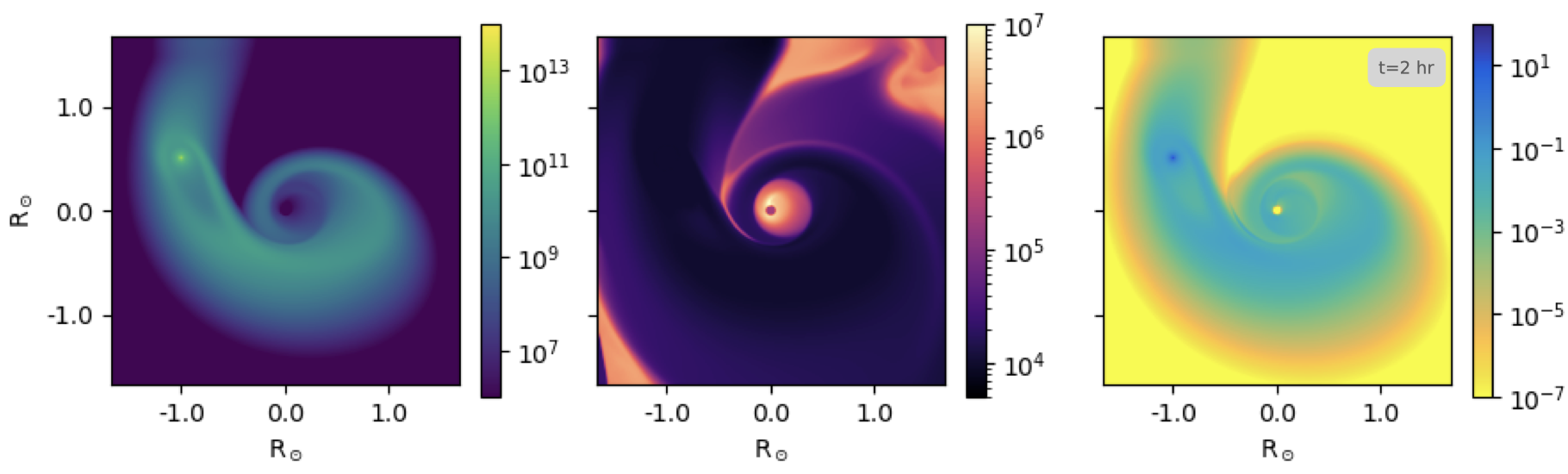
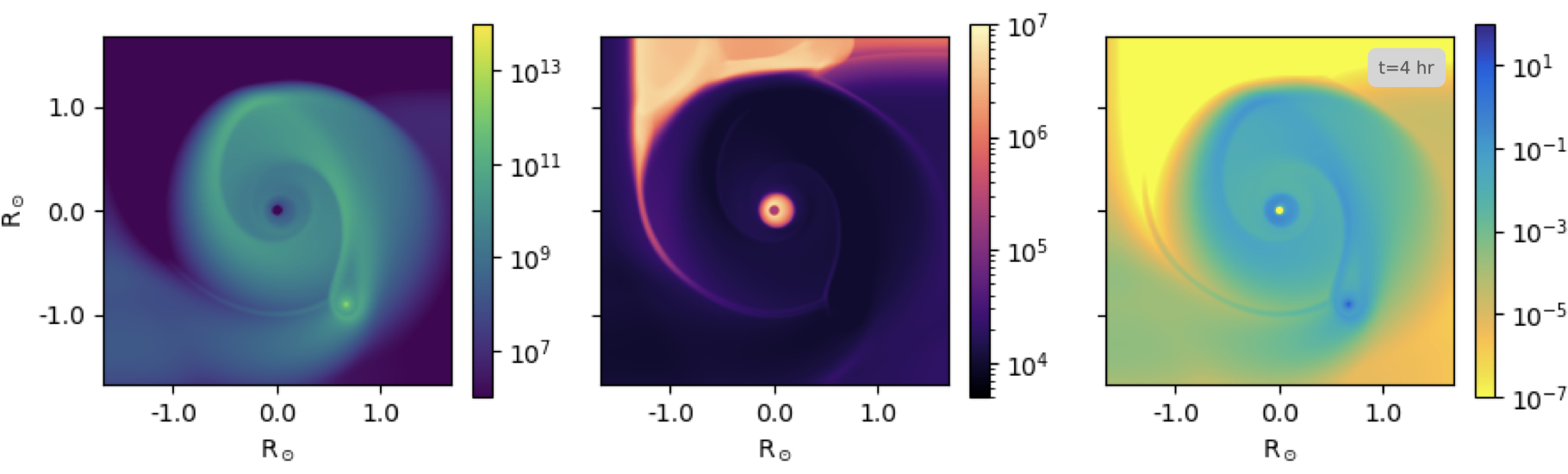
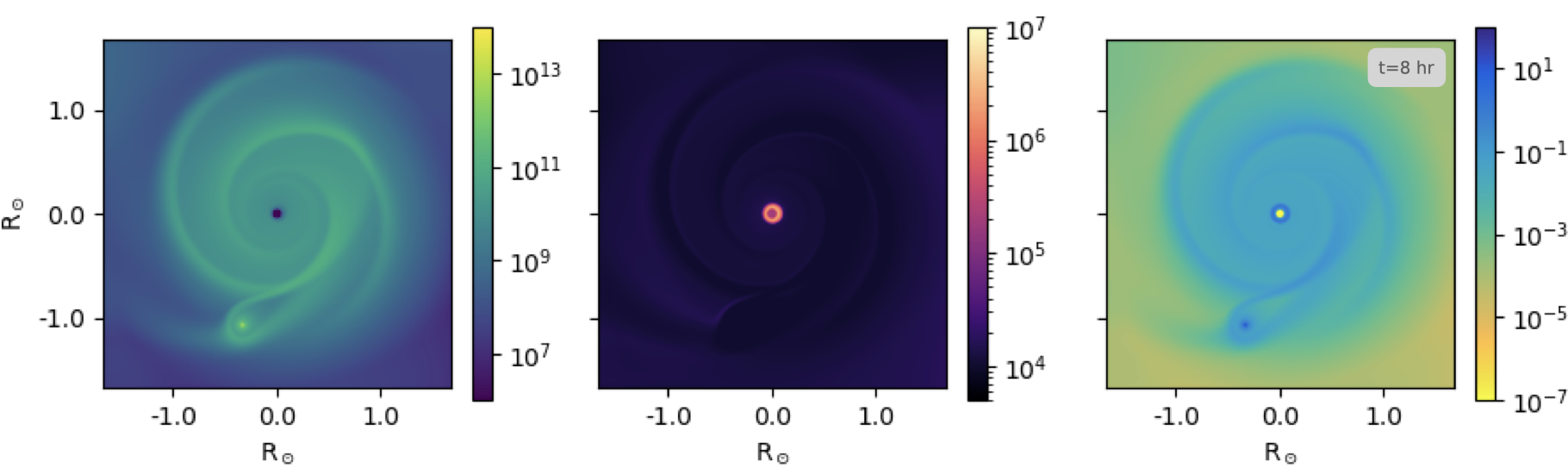
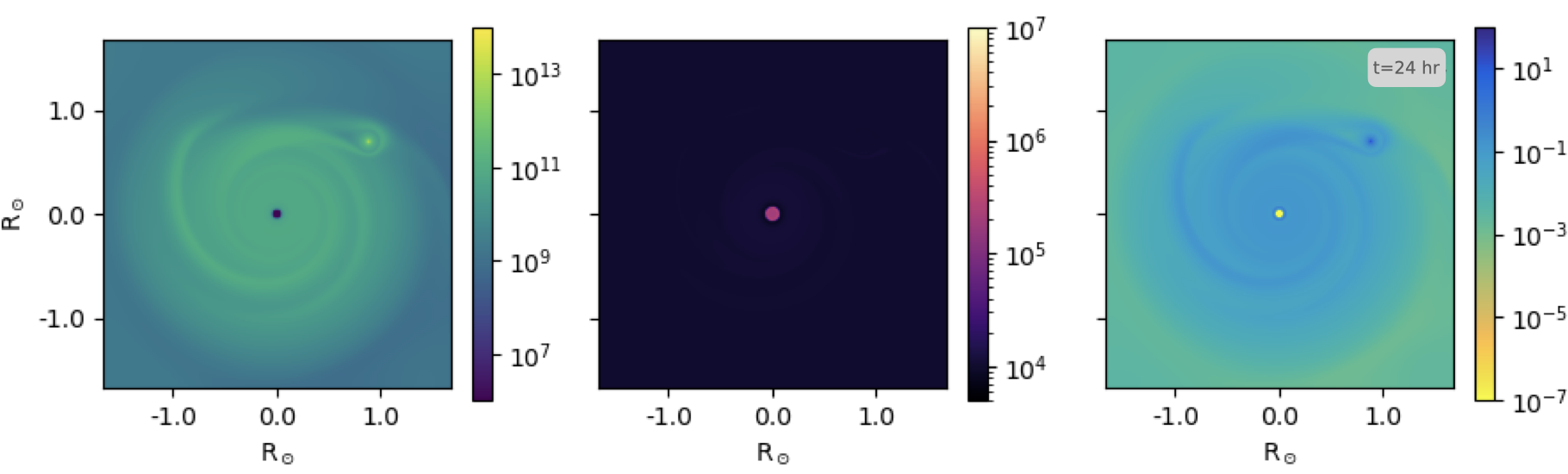
Figure 1: Face-on view of the middle plane of the number density $n$ (cm^-3 - left), temperature $T$ (K - middle) and pressure (erg cm^-3 - right) of Run A. From top to bottom we show the results after 2, 4, 8 and 24 hours of evolution, respectively.

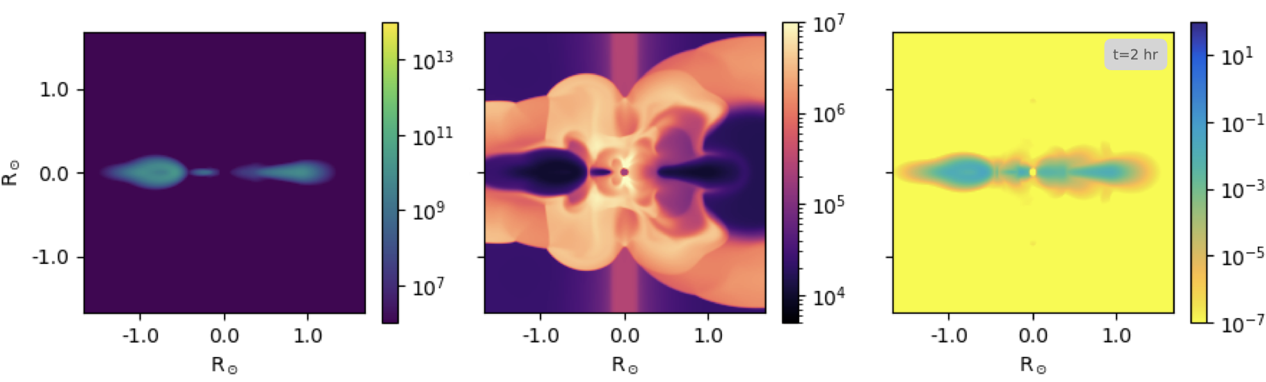
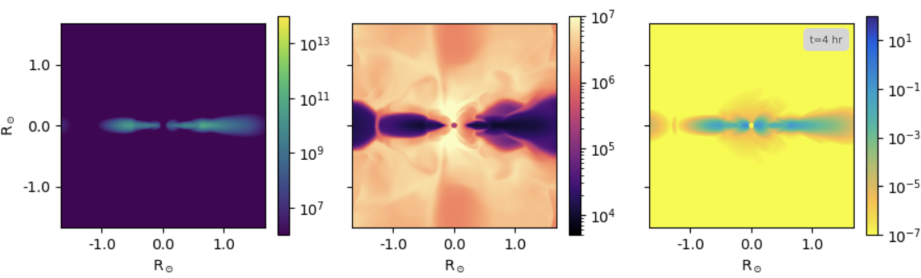
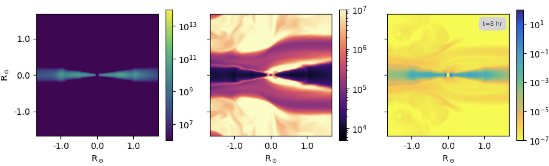
Figure 2: Same as Figure 1 for the edge-on view of the middle plane.

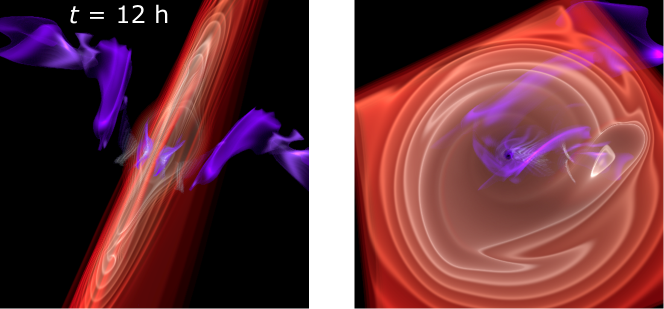
Figure 3: Visualization of rendered image of the accretion disk obtained from Run C after 12 h of evolution. The red shade represents material with number density in the 10⁹–10¹² cm^-3 range, whilst the purple strings represent material hot enough to produce hard X-rays ($T>10^{7}$ K). A video illustrating the formation and evolution of the disk is presented as supplementary material to this article.

The results from Run A are shown in Figures 1 and 2, which correspond respectively to the face-on and edge-on views of the number density $n$, temperature $T$ and pressure $p$. Note that the figures present cuts at the central plane and do not correspond to integrated images along the line of sight.

Figures 1 and 2 illustrate the early formation of an accretion disk around the WD. Material is lost by the orbiting Jupiter-like planet isotropically and is gravitationally-trapped by the WD. Fig. 1 shows that the gas does not fall directly into the WD, but spirals-in towards it creating spiral patterns of shocked gas. After 10 hours of evolution the disk around the WD reaches a steady state, with no further significant morphological changes.

Fig. 2 shows that once the disk is fully formed, its mid-plane region is composed by ionized material with temperatures of 10⁴ K surrounded by a thin layer of slightly higher temperatures ($\sim 10^{5}$ K). Material in the innermost regions of the disk can be extremely hot shocked up to X-ray-emitting temperatures of $\lesssim 10^{7}$ K (similar to the boundary layer of the accretion disk of dwarf novae and non-magnetic cataclysmic variables, Patterson & Raymond, 1985).

As illustration, Fig. 3 presents a 3D renderization of Run C after 12 h of the simulation, where the red shade represents material with density large enough, in the 10⁹–10¹² cm^-3 range, to create an accretion disk. On the other hand, the purple shade strings show material with temperature high enough to produce hard X-rays ($T>10^{7}$ K). This figure shows that X-ray-emitting gas is leaving the accretion disk but from the innermost regions, close to the WD. The X-ray-emitting material leaves the accretion disk in a bipolar stream of gas, but this is not collimated.

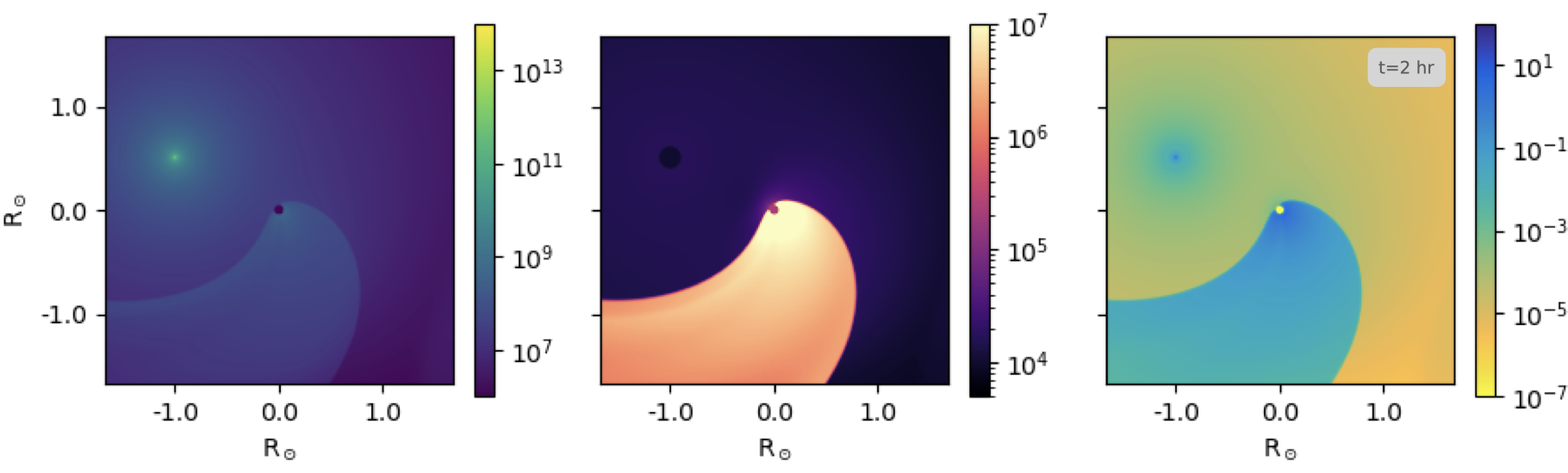
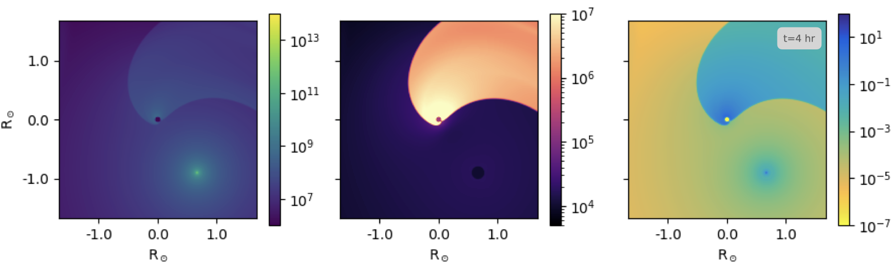
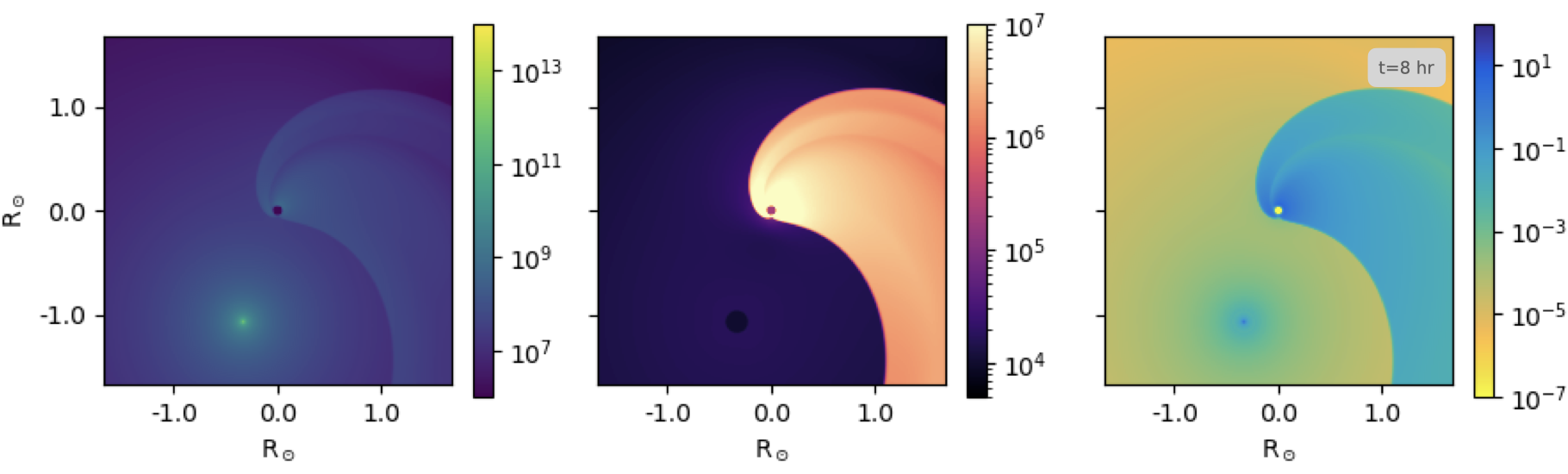
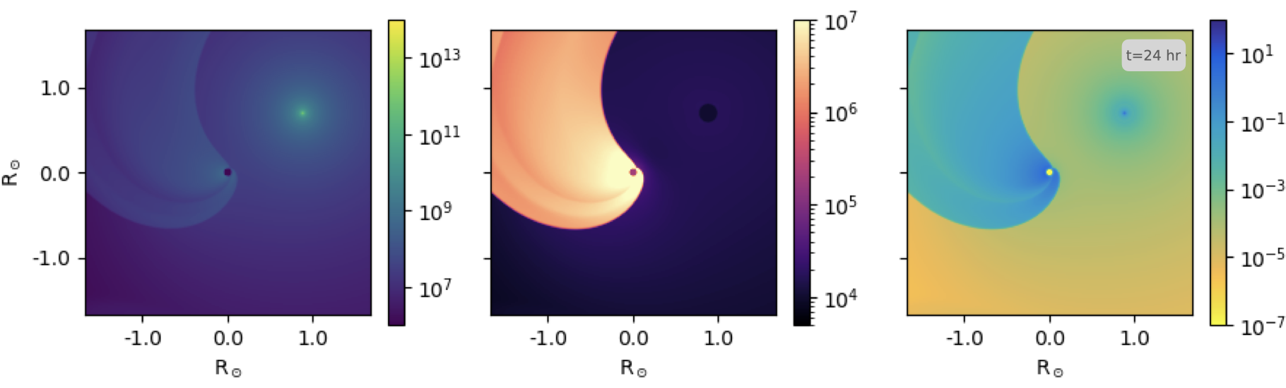
Figure 4: Same as Fig. 1 but for Run D.

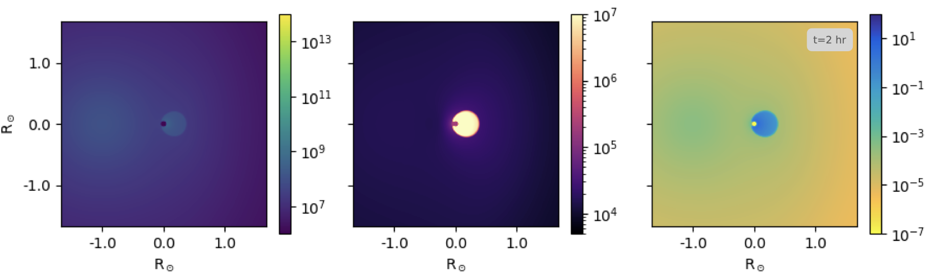
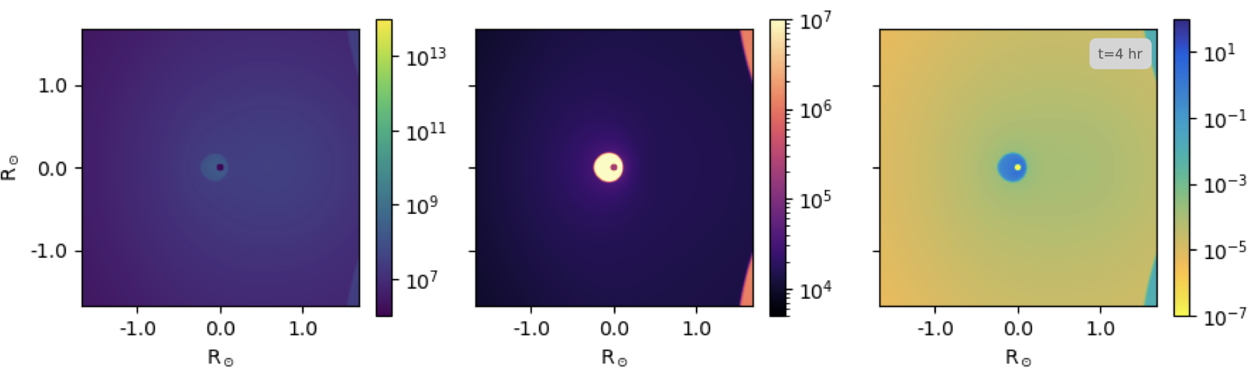
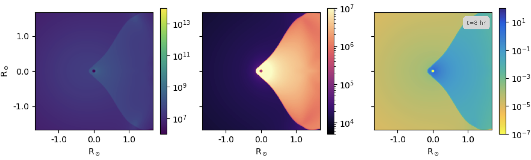
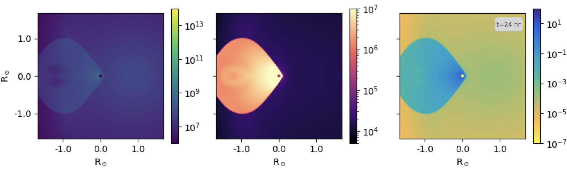
Figure 5: Same as Fig. 2 but for Run D.

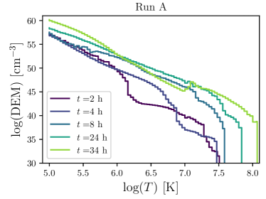
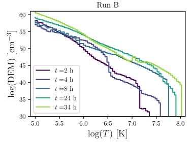
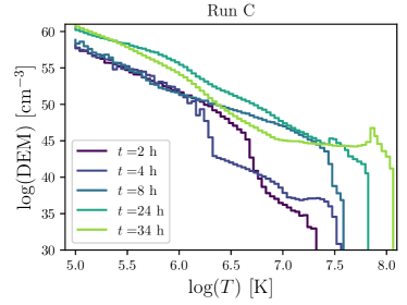
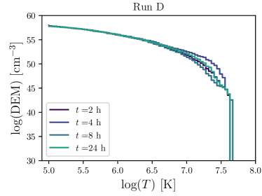
Figure 6: Differential emission measure (DEM) versus gas temperature ($T$) obtained for Run A (top left), B (top right), C (bottom left) and D (bottom right). The different line colours correspond to simulation results for different evolution times from 2 to 34 hr.

Figure 7: Synthetic X-ray spectra extracted from Run A using ChiantiPy. Different colours show spectra obtained for different snapshots of the simulation.

The results from Runs B and C, which have mass-loss rates 10 and 100 times larger than that adopted for Run A, but similar wind velocities, are presented in Appendix A. These simulations exhibit very similar morphological behaviour as that of Run A and will not be described further here. The main difference is the disk mass, which is higher for simulations with higher mass-loss rate from the Jupiter-like planet. These differences will have impact on the production of X-ray-emitting material (see below).

Other simulations with higher outflow velocity from the Jupiter-like planet were also attempted. In particular, we show here a simulation with the same mass-loss rate as that of Run A, but 10 times its outflowing velocity (600 km s^-1), labelled as Run D. The numerical results are presented in Fig. 4 and 5 for the face-on and edge-on views, respectively. In Run D the fast wind produces a lobe-shaped shocked region with the WD at its head. This structure is similar to a bow-shock produced by a star moving through the ISM (e.g., Green et al., 2022), but deformed following the circular orbit of the Jupiter-like planet.

3.1 Differential Emission Measure

In order to compare our results with those obtained from X-ray observations, we need to generate synthetic X-ray observations from our numerical results. However, we first need to characterise the properties of the X-ray-emitting material in the simulations. A useful tool is the differential emission measure (DEM).

Following Toalá & Arthur (2016, 2018), we define the DEM for each time step of the simulation as

$$\mathrm{DEM}(T_{\mathrm{b}})=\sum_{k,T_{\mathrm{k}}\in T_{\mathrm{b}}}n_{\mathrm{e}}^{2}\Delta V_{k},$$ (3)

where $n_{\mathrm{e}}$ is the electron number density in cell $k$, $\Delta V_{k}$ is the volume of cell $k$ and the sum is performed over cells with gas temperature falling in the bin whose central temperature is $T_{\mathrm{b}}$. In this work, we use logarithmic binning in the temperature range log($T$) = 5 to log($T$) = 9 in intervals of 0.04 dex (i.e., 100 bins). Lower temperatures are not taken into account in calculating the DEM, since their contribution to X-ray emission is negligible.

The DEM evolution with time corresponding to Runs A, B, C and D is illustrated in Fig 6. As expected, the DEM evolution of Runs A, B and C are very similar, but models with a higher mass-loss rate have higher DEM values. In the case of Run D, where no accretion disk is formed, the DEM profile does not change dramatically between different snapshots of the simulation.

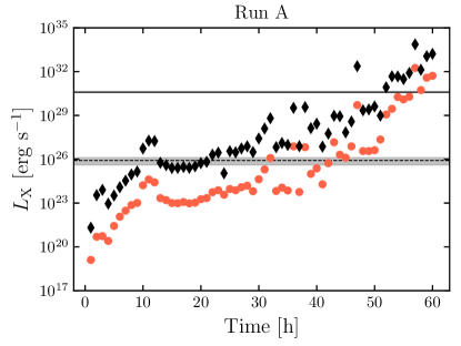
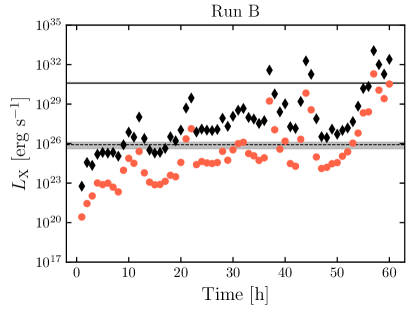
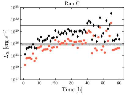
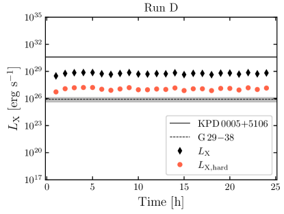
Figure 8: Synthetic X-ray luminosity versus time (light curves) computed for Run A (top left), B (top right), C (bottom left) and D (bottom right). The (black) diamonds and (orange) dots show the results for the total ($L_{\mathrm{X}}$) and hard ($L_{\mathrm{X,hard}}$) X-ray luminosities. The horizontal solid- and dashed-line show the X-ray luminosities of KPD 0005+5106 and G 29-38, respectively.

3.2 Synthetic X-ray emission

X-ray synthetic spectra are computed for each time and each simulation using the widely-tested Chianti database through the ChiantiPy routines (version 14.0; Dere, 2013; Dere et al., 2019).

The calculation performed by Chianti includes the contribution due to lines and to free-free, free-bound and two-photon continua. The abundances used to compute the spectra are those adopted for a standard ISM composition in Cloudy (version 17.0; Ferland et al., 2017). A spectrum is generated for each temperature bin and weighted by its appropriate DEM value. The synthetic spectrum is simply the sum of all these individual contributions. All synthetic spectra are computed in the 0.3–7.0 keV energy range, corresponding to the 1.7–40 Å  wavelength range. The calculations are performed with a spectral bin of 0.1 Å  and the spectral line full width half maximum adopted in this work is 0.01 Å.

Fig. 7 shows examples of the integrated spectrum that correspond to different snapshots of Run A taking into account times between 2 and 34 hr of evolution. The different spectral shapes are a direct reflection of the contribution of the DEM profiles. For example, the early DEM profile of Run A ($t$=2 h in the top left panel of Fig. 6) has a deficit of gas with temperatures higher than log($T$)=6.2 and this produces a spectrum dominated by emission with energies below 2 keV in Fig. 7. On the other hand, the DEM at 4 hr of Run A exhibits an increase of emission around log($T$)$\approx$6.5, which is reflected in an increase of emission for energies $>$2 keV in the spectrum as compared to that of the 2 hr of evolution. Similar spectral evolution patterns are exhibited by Runs B and C and are thus not shown here. Since the DEM profiles of Run D do not exhibit great differences, their resultant synthetic spectra are almost identical at all times.

The synthetic spectra can be used to estimate total ($L_{\mathrm{X}}$) and hard X-ray luminosities ($L_{\mathrm{X,hard}}$). These were obtained by integrating the synthetic spectra in the 0.3–7.0 keV and 0.6–7.0 keV energy ranges for $L_{\mathrm{X}}$ and $L_{\mathrm{X,hard}}$, respectively, which are the spectral ranges used in the analysis of the observations by Chu et al. (2021) and Estrada-Dorado et al. (2023). This procedure is also performed over all spectra obtained for the different snapshots of the simulations. Fig. 8 presents the evolution of the X-ray luminosity with time (or simply light curves) of the four simulations presented here. The (black) diamonds represent the evolution of $L_{\mathrm{X}}$ whilst the (orange) bullets represent $L_{\mathrm{X,hard}}$.

The first thing to notice is that the light curves do not reflect the variability of the orbital period of the Jupiter-like planet adopted in the simulation, which is 4.7 hr. Although certain variability is exhibited by the light curves of Runs A, B and C, these do not match the adopted period and, in fact, these are not consistent among them. The variability of the light curves is thus suggested to be stochastic caused by periods of enhanced accretion associated with instabilities of the disk as in dwarf novae (Warner, 1995). For discussion, Fig. 8 also shows in horizontal solid- and dashed-line the X-ray luminosity estimations corresponding to KPD 0005+5106 and G 29-38, respectively (see Estrada-Dorado et al., 2023; Chu et al., 2021). We note that the X-rays in runs A, B and C scales progressively in time, but it remains constant in simulation D where an accretion disk is not formed. Those simulations that generate an accretion disk reproduce reasonably the X-ray luminosity and spectral properties of G 29$-$38, but in the case of KPD 0005+5106, the luminosity is exceeded in a few moments of the late simulations. Due to the behaviour of the luminosities, those points that barely exceed the KPD 0005+5106 luminosity could be interpreted as flares in the accretion disk, which generate a drop in the emission after the peak. These are thus stochastic and not representative of the observed X-ray variable luminosity of KPD 0005+5106.

4 Discussion

The simulations presented here demonstrate that a WD is able to accrete material from a mass-losing planet and produce detectable X-ray emission. The synthetic X-ray fluxes predicted by our simulations are similar to those reported in the literature for X-ray-emitting evolved WDs accreting planetary material. Some details are worth discussing.

Runs A, B and C predict the formation of a relatively cold accretion disk. The X-ray-emitting material seems to be shock-heated at the inner regions of the disk and part of this material is subsequently ejected in the form of bipolar not-fully collimated outflow. The X-ray-emitting gas outflows and surrounds the accretion disk. In fact, the accretion disk has temperatures of a few times $10^{3}$ K, suggesting that this structure might contain hot dust.

It is interesting to note that the synthetic light curves presented in Fig. 8 do not reflect the orbital motion of the Jupiter-like planet around the WD adopted in the simulations. There is no clear pattern in the time evolution of the X-ray luminosity from Runs A, B or C. In fact, once the accretion disk is formed, the variability in the luminosity appears to be stochastic.

In order to assess the efficiency of the accretion process in our simulations, we calculated the accreted mass per unit of time of the simulation. This is illustrated for Runs A, B and C in Fig. 9. The evolution of the accreted mass per time of each simulation set is normalised to the planet’s mass-loss rate. Fig. 9 shows that at earlier times most of the mass is lost and not accreted by the WD given the isotropic nature of the wind from the planet. Once the accretion disk is formed ($\sim$10 hr) the efficiency reaches about 3 per cent. In the last 20 hr of the simulations, the accretion process has efficiency values between 18 and 25 per cent of the total mass lost by the planet. In later times of Runs A and B there is a couple of peaks in efficiency which we attribute to sudden accretion of material previously stripped from the planet. This figure confirms that the peaks in the light curves are also not related to the efficiency of the accretion process.

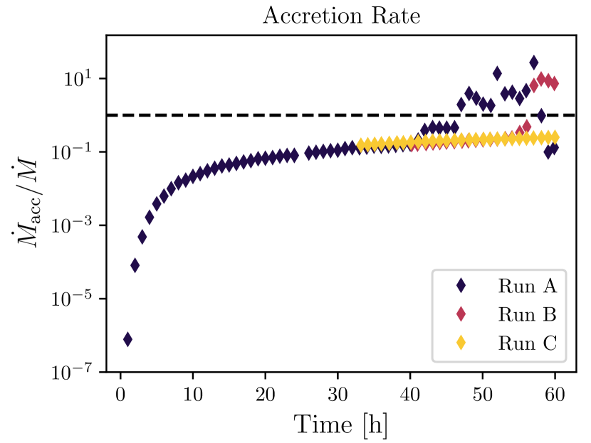
Figure 9: Evolution of the normalized accretion rate ($\dot{M}_{\mathrm{acc}}$) from the different simulations. Each simulation is normalized to its own mass-loss rate. The horizontal dashed-line represents an efficiency of 100 per cent.

The numerical results presented here are revealing and have consequences for KPD 0005+5106. Our simulations suggest that a scenario in which the variable hard X-ray emission is produced by accretion from planetary material onto a WD might not be capable of explaining the observed properties of KPD 0005+5106. Although at some times Runs A, B and C produce similar levels of X-ray emission, the presented simulations do not exhibit a clear periodic variability, which could be associated with that reported by the analysis of Chandra and XMM-Newton observations of this hot WD. Alternatively, the variable X-ray emission of KPD 0005+5106 can imply the presence of a hot-spot in the surface of the rotating star. According to Dupuis et al. (2000) a hot-spot in the WD is possible if the surface of the star has a concentration of metals which generate a chemical inhomogeneity. The presence of a magnetic field channelling the accretion onto the magnetic poles can also produce hot-spots as in polar or intermediate-polar binary systems. The variability would then be generated by the rotation of the WD in combination with the presence of a hot spot. This would mean that the rotation period of KPD 0005+5106 could be that reported for the hard X-ray emission (4.7 hr) which is consistent with the periods found for isolated WDs (see, e.g., Hermes et al., 2017).

The simulations presented here can also be used to discuss the X-ray emission detected from G 29-38. The dashed line presented in Fig. 8 at 10²⁵ erg s^-1 represents the X-ray luminosity from this WD (Estrada-Dorado et al., 2023). This means that the accretion disk scenario reproduces the emission of G 29-38, which is a polluted WD (Koester et al., 1997) with planetary debris (Cunningham et al., 2022) falling into the WD. This WD is one of the first metal-polluted WD where IR excess was associated with an accretion disk (Graham et al., 1990; Zuckerman & Becklin, 1987). The origin of such structure has been attributed to the presence of the disruption of an asteroid or a minor planet (Jura, 2003; Reach et al., 2005), but IR observations of this structure suggest that its chemical composition is better explained by material disrupted from a Jupiter-like planet according to Reach et al. (2009). In fact, a 4.4$\sigma$ detection of X-ray emission from G 29-38 has been used to suggest that this WD is accreting material from remnant planetary material (Cunningham et al., 2022). The latter has been corroborated by our team using XMM-Newton observations (see Estrada-Dorado et al., 2023). Except for Run D, the other three simulations predict similar X-ray luminosities and the formation of a relatively cold accretion disk, similar to what is found in G 29-38 (see Fig. 8).

5 Summary

We presented radiation-hydrodynamic simulations of the accretion of planetary material onto a WD. The simulations adopt the parameters (orbital period, accretion rate) estimated from the hard X-ray emission from the hot WD KPD 0005+5106. The simulations reproduce the formation of a relatively cold accretion disk around a WD with the X-ray emitting material leaving this disk mostly along the polar directions. The simulations predict X-ray luminosity levels similar to those reported in the literature from observations of the metal-polluted DAZ WD G 29$-$38, but marginally reproduce the hard X-ray emission for KPD 0005+5106 for certain times. The variability of the synthetic X-ray light curve does not follow the assumed orbital period, but is more likely stochastic. The X-ray emission basically grows with time until it reaches an asymptotic value when the accretion rate attains a steady value.

Consequently, we suggest that the variable hard X-ray emission detected from KPD 0005$+$5106 has another origin. We propose that it might be due to the presence of a hot spot on its surface most likely associated with the stellar magnetic field. The X-ray variability period would then be associated with the rotation period, which is most likely also the orbital period of a close companion as a close binary system will establish synchronous rotation. Further optical and X-ray monitoring is urged in order to further assess these characteristics.

Finally, we note that although the presented simulations were not tailored to the specific case of G 29-38, they are able to reproduce the observed X-ray luminosity level and the production of an accretion disk formed by planetary material as previously suggested. Given the low temperature of the accretion disk, we predict that it would contain host dust, which is another observable characteristic in G 29-38.

Data availability

The results of our simulations presented in this work are available in the article. Our results will be shared on reasonable request to the first author.

Appendix A Simulations B and C

In this appendix we present the hydrodynamical results of Runs B (Fig. 10 and 11) and C (Fig. 12 and 13). These simulations are very similar to those of Run A presented in Section 3 exhibiting the formation of the accretion disk around the WD (located at the centre of the numerical grid). Spiral arms of material spiraling in towards the accreting WD is disclosed by the face-on panels (see Fig. 10 and 12). Given that Runs B and C have 10 and 100 times higher mass-loss rate than Run A, respectively, the density of the accretion disks are higher that in that model. No other remarkable differences are produced.

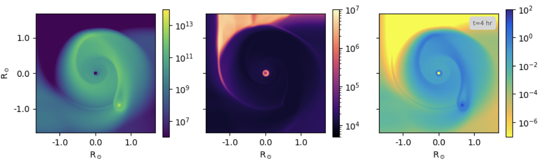
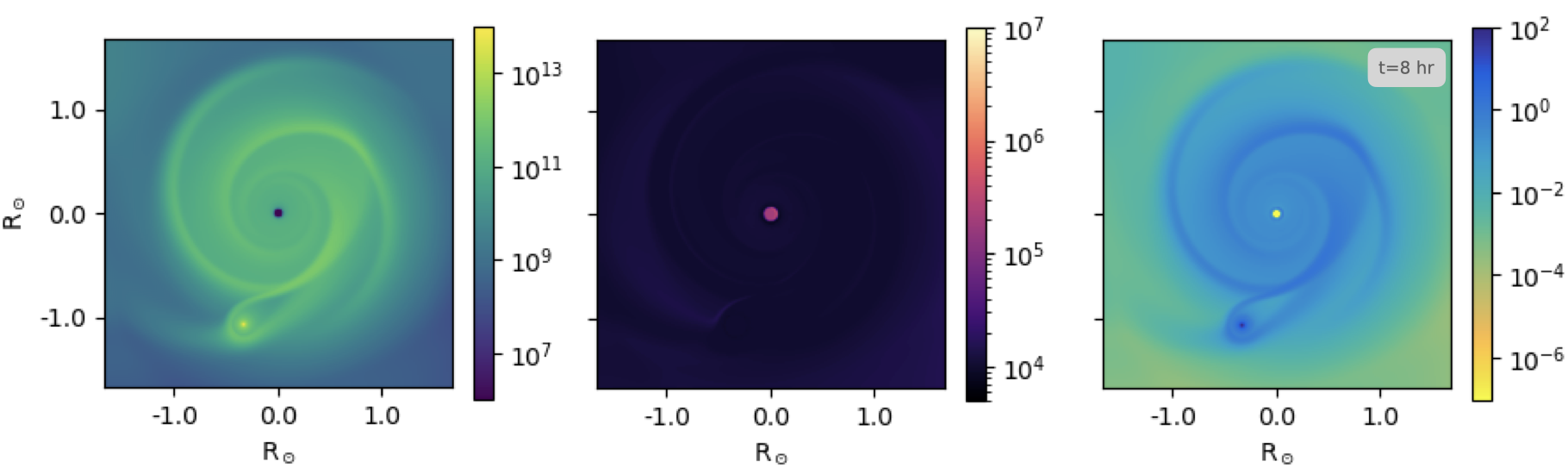
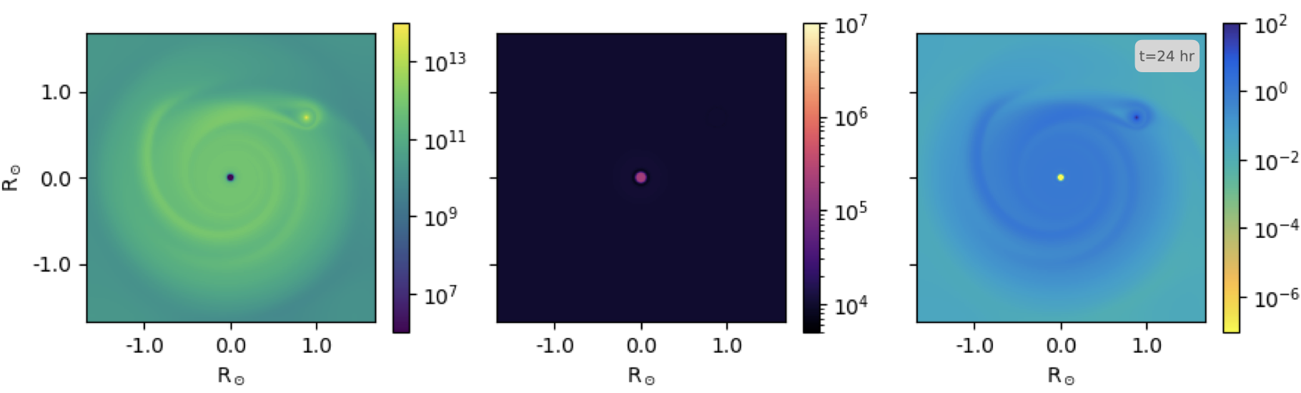
Figure 10: Face-on view of the middle plane of the number density $n$ (cm^-3 - left), temperature $T$ (K - middle) and pressure (erg cm^-3 - right) of Run B. From top to bottom we show show the results after 2, 4, 8 and 24 hrs of evolution.

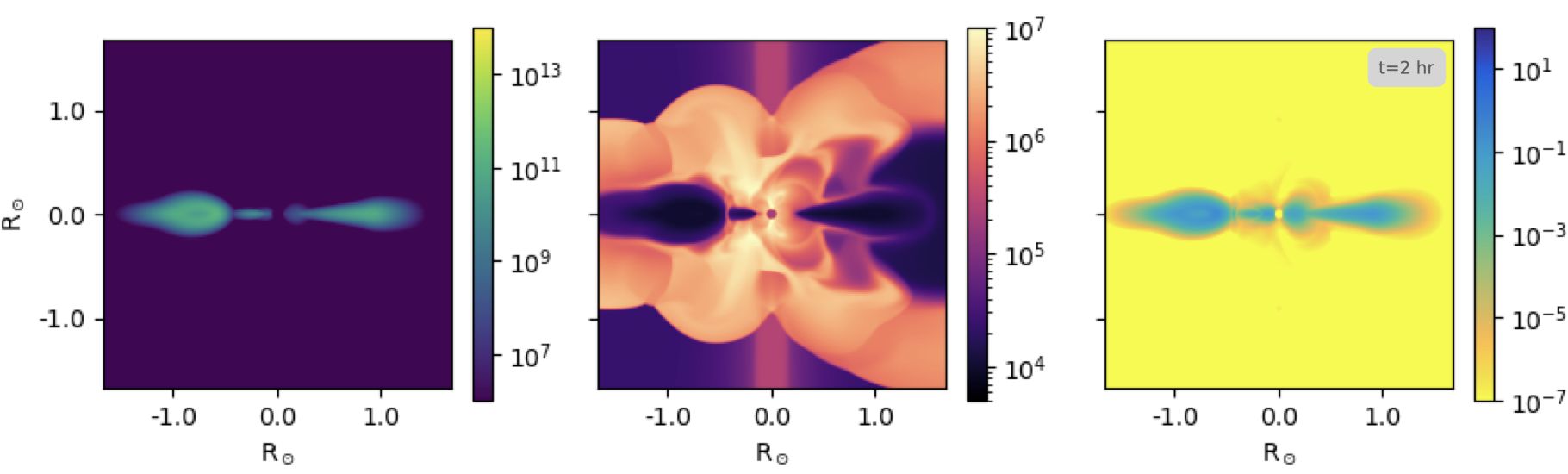
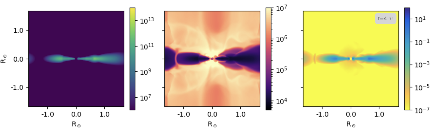
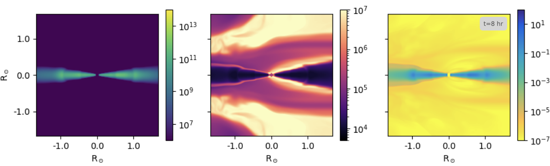
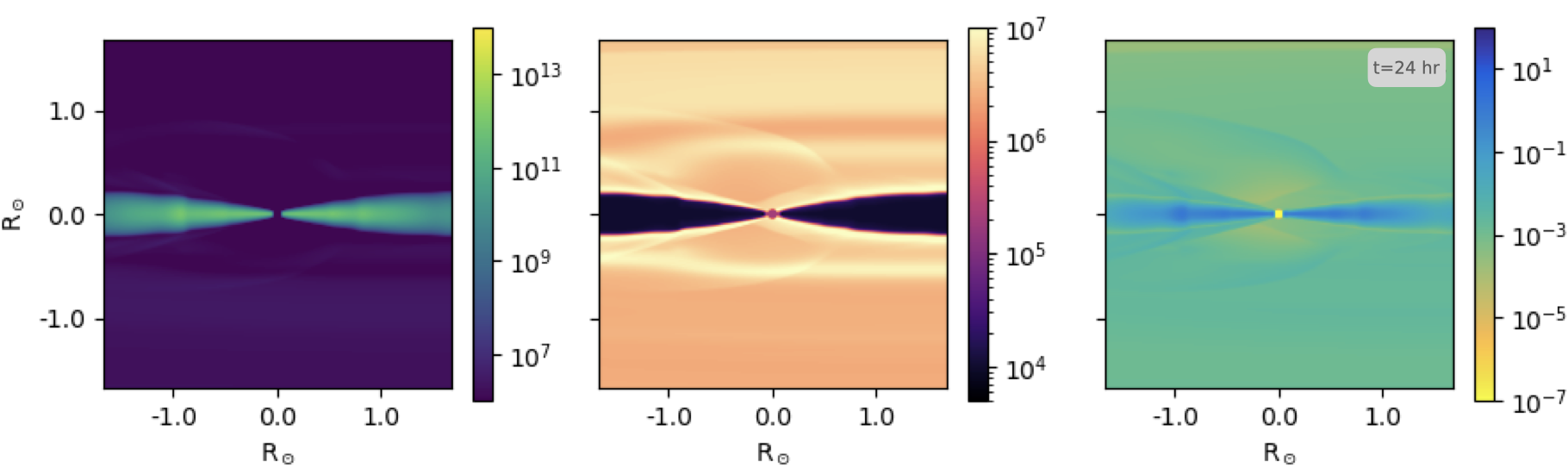
Figure 11: Edge-on view of the middle plane of the number density $n$ (cm^-3 - left), temperature $T$ (K - middle) and pressure (erg cm^-3 - right) of Run B. From top to bottom we show show the results after 2, 4, 8 and 24 hrs of evolution.

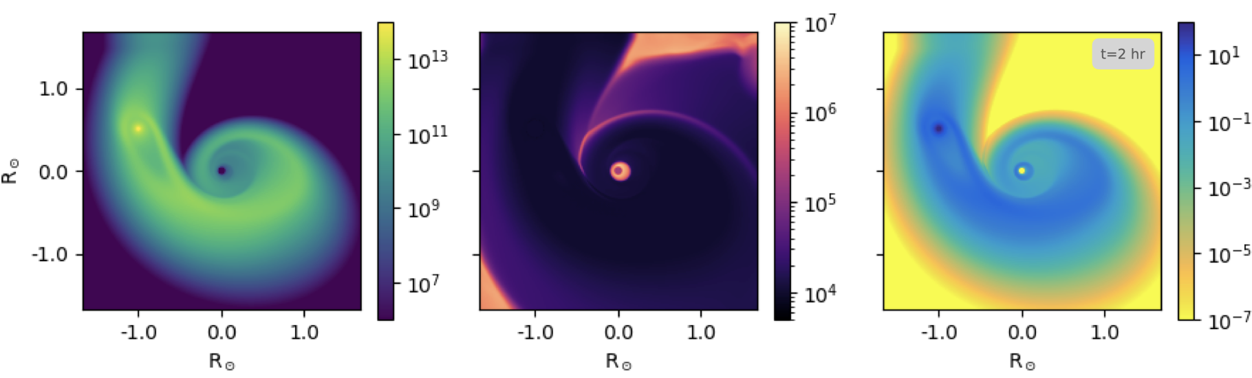
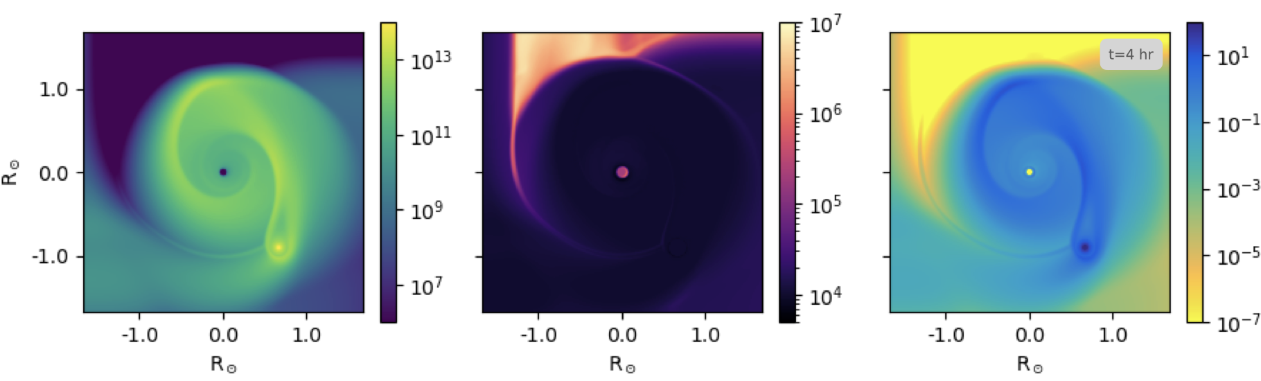
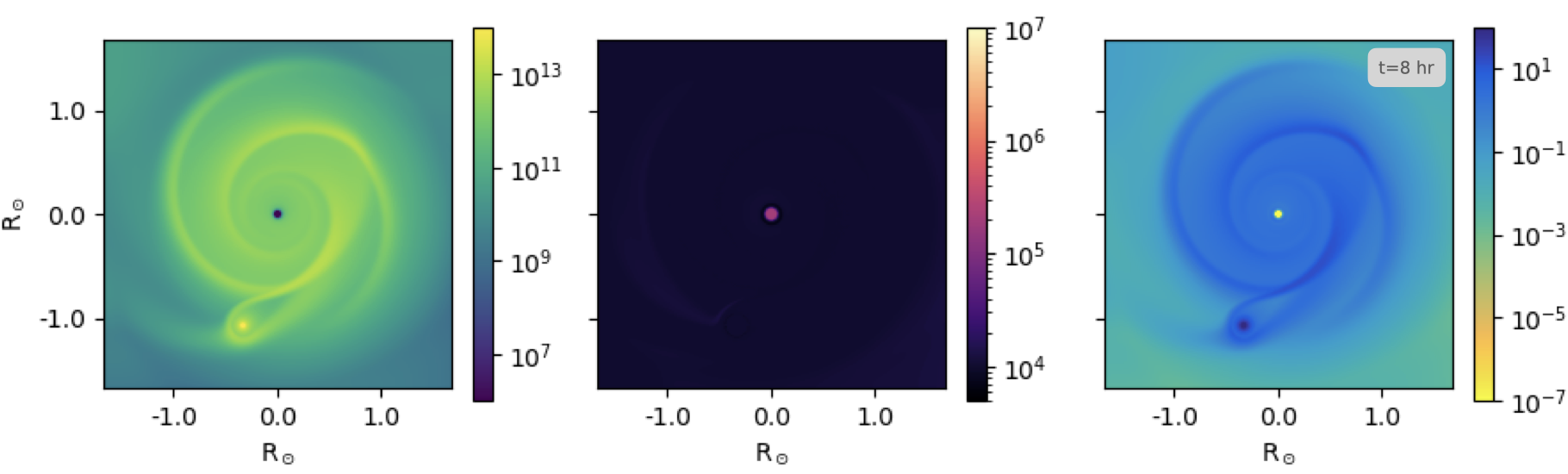
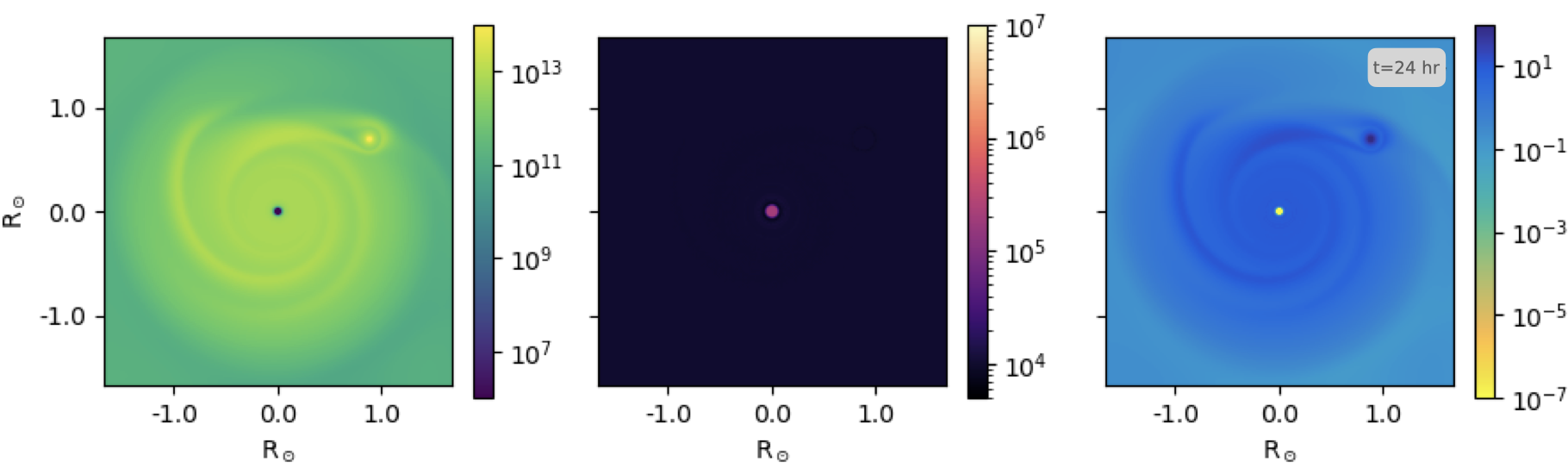
Figure 12: Face-on view of the middle plane of the number density $n$ (cm^-3 - left), temperature $T$ (K - middle) and pressure (erg cm^-3 - right) of Run C. From top to bottom we show show the results after 2, 4, 8 and 24 hrs of evolution.

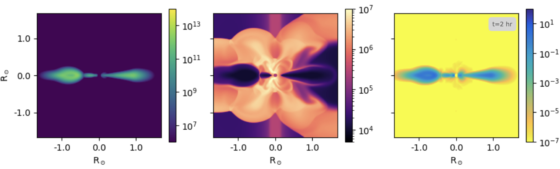
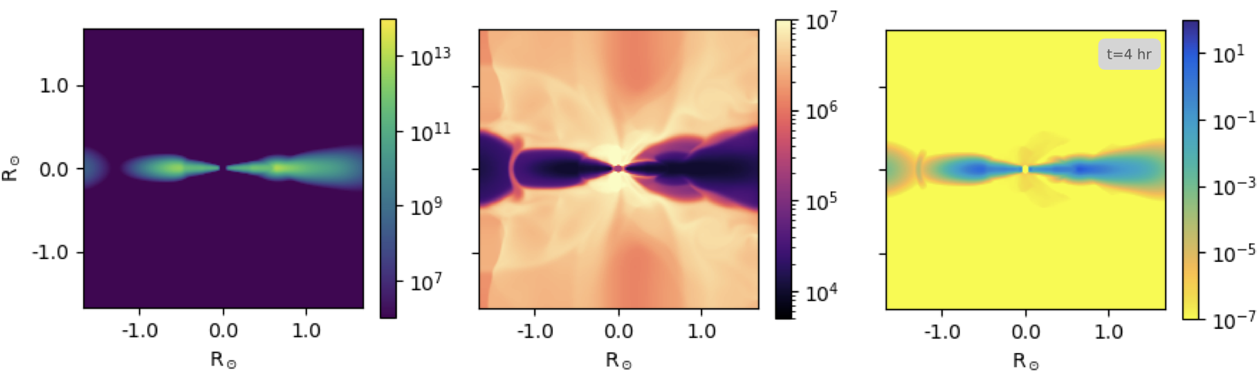
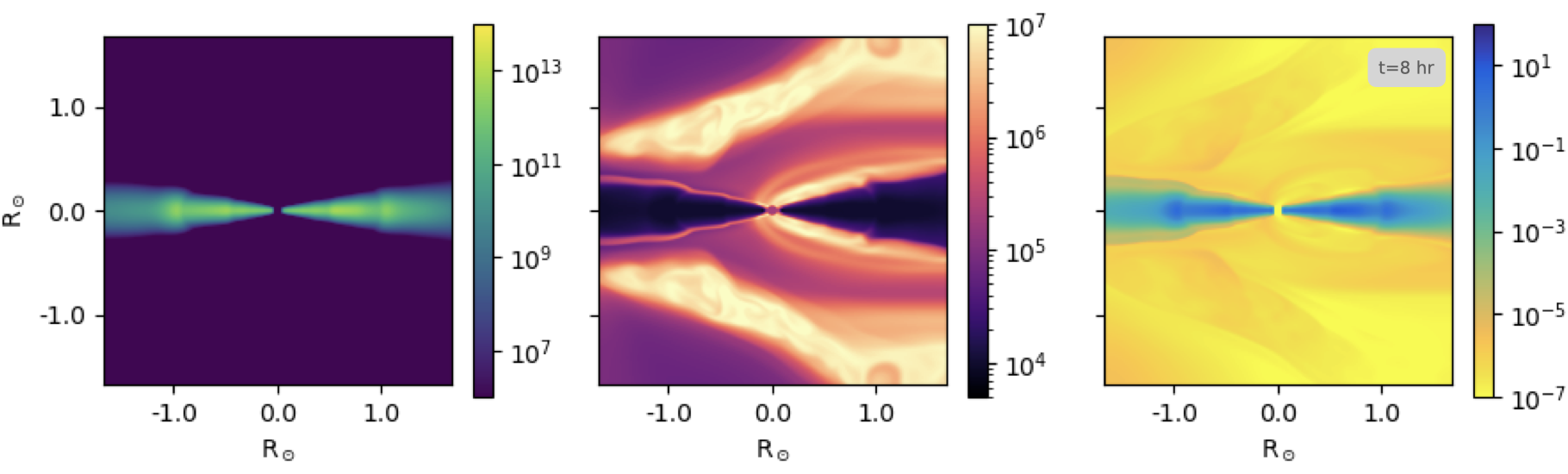
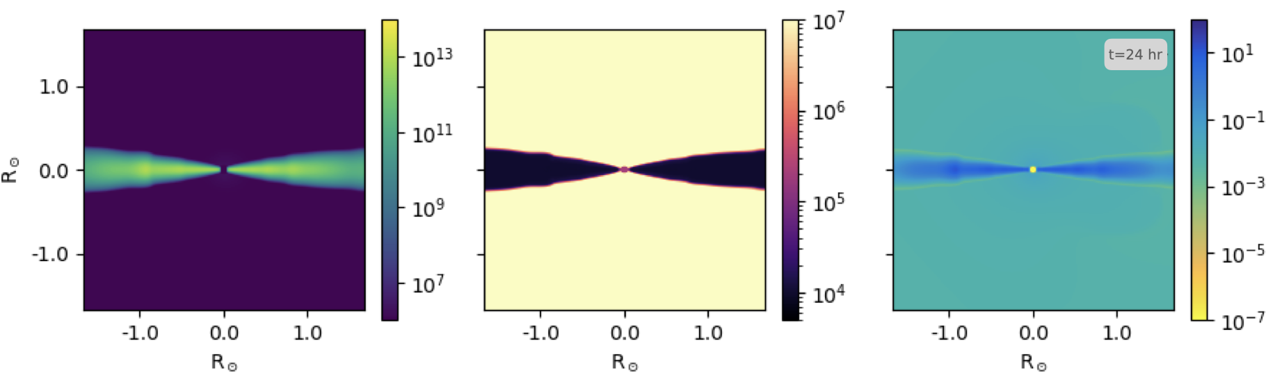
Figure 13: Edge-on view of the middle plane of the number density $n$ (cm^-3 - left), temperature $T$ (K - middle) and pressure (erg cm^-3 - right) of Run C. From top to bottom we show show the results after 2, 4, 8 and 24 hrs of evolution.

References

- Alonso et al. (2021) Alonso, R., Rodríguez-Gil, P., Izquierdo, P., et al. 2021, A&A, 649, A131
- Bilíková et al. (2010) Bilíková, J., Chu, Y.-H., Gruendl, R. A., et al. 2010, AJ, 140, 1433
- Bilíková et al. (2012) Bilíková, J., Chu, Y.-H., Gruendl, R. A., et al. 2012, ApJS, 200, 3. doi:10.1088/0067-0049/200/1/3
- Blackman et al. (2021) Blackman, J. W., Beaulieu, J. P., Bennett, D. P., et al. 2021, Nature, 598, 272
- Brandner et al. (2021) Brandner, W., Zinnecker, H., & Kopytova, T. 2021, MNRAS, 500, 3920
- Chu et al. (2021) Chu, Y.-H., Toalá, J. A., Guerrero, M. A., et al. 2021, ApJ, 910, 119. doi:10.3847/1538-4357/abe5a5
- Chu et al. (2004a) Chu, Y.-H., Guerrero, M. A., Gruendl, R. A., et al. 2004, AJ, 127, 477
- Cunningham et al. (2022) Cunningham, T., Wheatley, P. J., Tremblay, P.-E., et al. 2022, Nature, 602, 219. doi:10.1038/s41586-021-04300-w
- Del Zanna et al. (2021) Del Zanna, G., Dere, K. P., Young, P. R., et al. 2021, ApJ, 909, 38. doi:10.3847/1538-4357/abd8ce
- Dere (2013) Dere, K. 2013, Astrophysics Source Code Library. ascl:1308.017
- Dere et al. (2019) Dere, K. P., Del Zanna, G., Young, P. R., et al. 2019, ApJS, 241, 22. doi:10.3847/1538-4365/ab05cf
- Dupuis et al. (2000) Dupuis, J., Chayer, P., Vennes, S., et al. 2000, ApJ, 537, 977. doi:10.1086/309079
- Farihi et al. (2010) Farihi, J., Barstow, M.A., et al. 2010, MNRAS, 404, 2123.
- Fitzmaurice et al. (2023) Fitzmaurice, E., Martin, D. V., Rodríguez Martínez, R., et al. 2023, MNRAS, 518, 636. doi:10.1093/mnras/stac2879
- Estrada-Dorado et al. (2023) Estrada-Dorado, S., Guerrero, M. A., Toalá, J. A., et al. 2023, ApJ, 944, L46. doi:10.3847/2041-8213/acba7e
- Esquivel et al. (2009) Esquivel, A., Raga, A. C., Cantó, J., et al. 2009, A&A, 507, 855. doi:10.1051/0004-6361/200912825
- Esquivel & Raga (2013) Esquivel, A. & Raga, A. C. 2013, ApJ, 779, 111. doi:10.1088/0004-637X/779/2/111
- Ferland et al. (2017) Ferland, G. J., Chatzikos, M., Guzmán, F., et al. 2017, Rev. Mex. Astron. Astrofis., 53, 385
- Graham et al. (1990) Graham, J. R., Matthews, K., Neugebauer, G., et al. 1990, ApJ, 357, 216. doi:10.1086/168907
- Green et al. (2022) Green, S., Mackey, J., Kavanagh, P., et al. 2022, A&A, 665, A35. doi:10.1051/0004-6361/202243531
- Guerrero et al. (2001) Guerrero, M. A., Chu, Y.-H., Gruendl, R. A., et al. 2001, ApJ, 553, L55. doi:10.1086/320509
- Guerrero & De Marco (2013) Guerrero, M. A. & De Marco, O. 2013, A&A, 553, A126. doi:10.1051/0004-6361/201220623
- Hansen et al. (2006) Hansen, B. M. S., Kulkarni, S., & Wiktorowicz, S. 2006, AJ, 131, 1106. doi:10.1086/499207
- Hermes et al. (2017) Hermes, J. J., Gänsicke, B. T., Kawaler, S. D., et al. 2017, ApJS, 232, 23. doi:10.3847/1538-4365/aa8bb5
- Holberg & Howell (2011) Holberg, J. B. & Howell, S. B. 2011, AJ, 142, 62. doi:10.1088/0004-6256/142/2/62
- Jura (2003) Jura, M. 2003, ApJ, 584, L91. doi:10.1086/374036
- Jura (2008) Jura, M. 2008, AJ, 135, 1785.
- Koester et al. (1997) Koester, D., Provencal, J., & Shipman, H. L. 1997, A&A, 320, L57
- Kosakowski et al. (2022) Kosakowski, A., Kilic, M., Brown, W. R., et al. 2022, MNRAS. doi:10.1093/mnras/stac1146
- Kwok (2000) Kwok, S. 2000, The origin and evolution of planetary nebulae / Sun Kwok. Cambridge; New York: Cambridge University Press, 2000. (Cambridge astrophysics series ; 33)
- Martin et al. (2021) Martin, D. V., El-Badry, K., Hodžić, V. K., et al. 2021, MNRAS, 507, 4132
- O’Dwyer et al. (2003) O’Dwyer, I. J., Chu, Y.-H., Gruendl, R. A., et al. 2003, AJ, 125, 2239
- Patterson & Raymond (1985) Patterson J., Raymond J. C., 1985, ApJ, 292, 535. doi:10.1086/163187
- Privitera et al. (2016) Privitera, G., Meynet, G., Eggenberger, P., et al. 2016, A&A, 593, A128
- Raga et al. (2009) Raga, A. C., Henney, W., Vasconcelos, J., et al. 2009, MNRAS, 392, 964. doi:10.1111/j.1365-2966.2008.14097.x
- Rao et al. (2021) Rao, S., Pezzotti, C., Meynet, G., et al. 2021, A&A, 651, A50
- Reach et al. (2009) Reach, W. T., Lisse, C., von Hippel, T., et al. 2009, ApJ, 693, 697. doi:10.1088/0004-637X/693/1/697
- Reach et al. (2005) Reach, W. T., Kuchner, M. J., von Hippel, T., et al. 2005, ApJ, 635, L161. doi:10.1086/499561
- Schneiter et al. (2016) Schneiter, E. M., Esquivel, A., Villarreal D’Angelo, C. S., et al. 2016, MNRAS, 457, 1666. doi:10.1093/mnras/stw076
- Scicluna et al. (2022) Scicluna, P., Kemper, F., McDonald, I., et al. 2022, MNRAS, 512, 1091. doi:10.1093/mnras/stab2860
- Stephan et al. (2020) Stephan, A. P., Naoz, S., Gaudi, B. S., et al. 2020, ApJ, 889, 45. doi:10.3847/1538-4357/ab5b00
- Su et al. (2007) Su, K. Y. L., Chu, Y.-H., Rieke, G. H., et al. 2007, ApJ, 657, L41. doi:10.1086/513018
- Toalá & Arthur (2016) Toalá, J. A. & Arthur, S. J. 2016, MNRAS, 463, 4438. doi:10.1093/mnras/stw2307
- Toalá & Arthur (2018) Toalá, J. A. & Arthur, S. J. 2018, MNRAS, 478, 1218. doi:10.1093/mnras/sty1127
- Toro et al. (1994) Toro, E. F., Spruce, M., & Speares, W. 1994, Shock Waves, 4, 25. doi:10.1007/BF01414629
- Van Grootel et al. (2021) Van Grootel, V., Pozuelos, F. J., Thuillier, A., et al. 2021, A&A, 650, A205
- van Roestel et al. (2021) van Roestel, J., Kupfer, T., Bell, K. J., et al. 2021, ApJ, 919, L26
- Vanderburg et al. (2020) Vanderburg, A., Rappaport, S. A., Xu, S., et al. 2020, Nature, 585, 363
- Veras (2021) Veras, D. 2021, Oxford Research Encyclopedia of Planetary Science, 1. doi:10.1093/acrefore/9780190647926.013.238
- Villaver & Livio (2007) Villaver, E. & Livio, M. 2007, ApJ, 661, 1192
- Walters et al. (2022) Walters, N., Farihi, J., Marsh, T. R., et al. 2022, arXiv:2207.07022
- Warner (1995) Warner, B. 1995, Ap&SS, 230, 83. doi:10.1007/BF00658170
- Werner & Rauch (2015) Werner, K. & Rauch, T. 2015, A&A, 583, A131. doi:10.1051/0004-6361/201527212
- Xu et al. (2020) Xu, S., Lai, S., & Dennihy, E. 2020, ApJ, 902, 127. doi:10.3847/1538-4357/abb3fc
- Zuckerman & Becklin (1987) Zuckerman, B. & Becklin, E. E. 1987, Nature, 330, 138. doi:10.1038/330138a0