Impact of moment-based, energy integrated neutrino transport on microphysics and ejecta in binary neutron star mergers

Abstract

We present an extensive study of the effects of neutrino transport in 3-dimensional general relativistic radiation hydrodynamics (GRHD) simulations of binary neutron star (BNS) mergers using our moment-based, energy-integrated neutrino radiation transport (M1) scheme. We consider a total of 8 BNS configurations, while varying equation of state models, mass ratios and grid resolutions, for a total of 16 simulations. We find that M1 neutrino transport is crucial in modeling the local absorption of neutrinos and the deposition of lepton number throughout the medium. We provide an in-depth look at the effects of neutrinos on the fluid dynamics and luminosity during the late inspiral and post-merger phases, the properties of ejecta and outflow, and the post-merger nucleosynthesis. The simulations presented in this work comprise an extensive study of the combined effect of the equation of state and M1 neutrino transport in GRHD simulations of BNS mergers, and establish that the solution provided by our M1 scheme is robust across system properties and provides insight into the effects of neutrino trapping in BNS mergers.

I Introduction

As we approach the era of precision gravitational wave astronomy Amaro-Seoane et al. (2017); Sathyaprakash et al. (2019); Maggiore et al. (2020); Adhikari et al. (2019); Bellovary et al. (2020); Abbott et al. (2021); Ballmer et al. (2022); Berti et al. (2022); Buonanno et al. (2022), the need for high-accuracy numerical simulations of binary neutron star (BNS) mergers becomes ever relevant Duez and Zlochower (2019); Tsokaros and Uryū (2022); Foucart et al. (2022a). There is presently a concerted effort to improve the accuracy and proper treatment of relevant physical phenomena in numerical relativity (NR) codes, including: (1) the accuracy associated with gravitational waves (GWs) extracted from simulations, which inform matched-filtered searches in current and future GW detectors Chu et al. (2016); Bernuzzi and Dietrich (2016); Most et al. (2019a); Westernacher-Schneider (2021); Poudel et al. (2020); Dudi et al. (2022); Doulis et al. (2022); (2) the methods used for treating radiation and neutrino transport Sekiguchi et al. (2015); Radice et al. (2018a); Nedora et al. (2021a); Vincent et al. (2020); Weih et al. (2020); Foucart et al. (2020); Radice et al. (2022); (3) the accurate treatment of magnetic field effects Paschalidis et al. (2015); Ruiz et al. (2018, 2016); Kiuchi et al. (2018); Shibata et al. (2021); Ciolfi and Kalinani (2020); Mosta et al. (2020); Ciolfi (2020); and (4) the neutron star (NS) equation of state (EOS) Abdikamalov et al. (2009); Bauswein et al. (2013a); Palenzuela et al. (2015); Sekiguchi et al. (2015); Lehner et al. (2016); Radice et al. (2018a); Most et al. (2019b); Dietrich et al. (2018); Vincent et al. (2020). NR simulations of BNS mergers stand as our best tools for understanding the complex interactions of all of the aforementioned phenomena and effects during different stages of the merger process. However, substantial work remains to be done to improve the accuracy and microphysics within NR codes Foucart et al. (2022a).

An area of particular interest is the accurate treatment of neutrino transport in NR simulations. Different stages of a BNS merger are expected to produce intense neutrino emission. A burst of relatively low energy neutrinos (with energy $E_{\nu}\sim\mathcal{O}(\text{MeV})$) is expected during the formation of the central remnant Eichler et al. (1989); Rosswog and Liebendoerfer (2003). Higher energy neutrinos $E_{\nu}\sim\mathcal{O}(\text{TeV})$ may also be produced by hadronic interactions within the relativistic jet that forms after the merger Fang and Metzger (2017); Kimura et al. (2018). Thermal neutrinos ($E_{\nu}\sim\mathcal{O}(\text{MeV})$) are also expected from the cooling of long-lived (with lifetimes longer than $t\sim\mathcal{O}(\text{s})$), post-merger NS remnants Kyutoku and Kashiyama (2018). It may even be possible to detect very-high energy ($E_{\nu}\sim\mathcal{O}(\text{EeV})$) neutrinos on a timescale of days to weeks after merger, in the event that a long-lived magnetar remnant is produced Murase et al. (2009); Fang and Metzger (2017). The peak neutrino luminosity during a BNS merger is typically $L_{\nu}\sim 10^{53}-10^{54}$\text{\,}\mathrm{e}\mathrm{r}\mathrm{g}\mathrm{/}\mathrm{s}$$, which is a few times greater than that associated with core-collapse supernovae (CCSNe)  Ruffert et al. (1997); Rosswog and Liebendoerfer (2003); Sekiguchi et al. (2015); Palenzuela et al. (2015); Foucart et al. (2016a, b); Wu et al. (2017); George et al. (2020); Burrows et al. (2020); Kullmann et al. (2022); Cusinato et al. (2021); Radice et al. (2022).

During different stages of the merger, regions of the system can be in a state that is anywhere from the optically thin regime (wherein neutrinos free-stream) to the optically thick regime (wherein neutrinos diffuse) Endrizzi et al. (2020). In all of these scenarios, due to their large energies and luminosities, neutrinos are expected to play an important role. The impact of neutrinos is especially relevant in the environment following a BNS merger. For example, in the diffusive limit, neutrino interactions are expected to change the matter composition. A changing matter composition is relevant for determining the conditions relevant for $r$-process nucleosynthesis Lattimer and Schramm (1974); Just et al. (2015); Thielemann et al. (2017); Perego et al. (2021); Radice et al. (2022) and may also emergently lead to dissipation in out-of-equilibrium fluid dynamics Alford et al. (2018); Hammond et al. (2021); Most et al. (2022); Celora et al. (2022); Chabanov and Rezzolla (2023); Espino et al. (2023). Neutrinos that are produced in the hot and dense regions may reach the conditions for decoupling and may eventually be emitted from the system, thereby carrying off energy Rosswog et al. (1999). As the neutrinos remove energy from the system, they may lead to additional matter outflow in the form of neutrino-driven winds Rosswog et al. (1999); Rosswog and Ramirez-Ruiz (2002); Dessart et al. (2009); Perego et al. (2014); Radice et al. (2018b); Nedora et al. (2021a). Even in the free-streaming limit neutrino irradiation may significantly change the composition of the low-density regions of the remnant and ejecta via charged-current interactions Dessart et al. (2009); Perego et al. (2014); Just et al. (2015); Foucart et al. (2016a); Sekiguchi et al. (2016, 2016).

Capturing the aforementioned effects in BNS mergers simulations requires a sufficiently accurate treatment of neutrino transport in NR codes, which in principle requires a solution to the Boltzmann equations of radiation transport. Full solutions to the Boltzmann equation require the evolution of a 7-dimensional distribution function for each species of neutrino considered, which presents a computationally intensive problem. Many alternative approaches for capturing the effects of neutrino transport have been considered in the context of BNS merger simulations, including both direct and approximate methods. For example, some modern methods that directly tackle the solution of the Boltzmann equation include the expansion of momentum-space distributions into spherical harmonics Radice et al. (2013), lattice-Boltzmann based methods Weih et al. (2020), Monte Carlo (MC)-based methods Abdikamalov et al. (2012); Richers et al. (2015); Ryan et al. (2015); Foucart (2018); Foucart et al. (2018, 2020, 2021), and discrete-ordinates-based methods Nagakura (2022). Compared to approximate methods, direct methods are generally more accurate and suffer less from model-dependence; on the other hand, they are often complex to implement into numerical codes and computationally intensive. For instance, MC-based methods may become prohibitively expensive in the optically thick regime, where the neutrino mean-free path (which must be resolved to properly capture neutrino-matter thermal equilibrium) becomes small. Recent developments in the use of MC-based schemes address the need for prohibitive amount of MC particles by modifying the relevant interaction rates in regions of high optical depth, such that the neutrino energy distribution is unaffected close to regions where the neutrinos decouple from the matter Foucart et al. (2020, 2021). Such an approach may reliably capture the effects of neutrinos in the optically thin and optically thick limits but cannot do so for the emergent out-of-equilibrium effects captured by a fluid treatment of the radiation Alford et al. (2018); Hammond et al. (2021); Most et al. (2022); Celora et al. (2022); Chabanov and Rezzolla (2023); Espino et al. (2023).

Approximate methods to the solution of the Boltzmann equation model the relevant effects of neutrino transport in BNS mergers while reducing computational expense. For example, neutrino leakage schemes Sekiguchi (2010); Sekiguchi et al. (2011); O’Connor and Ott (2010); Wanajo et al. (2014); Foucart et al. (2016b); Radice et al. (2016); Perego et al. (2017a); Ardevol-Pulpillo et al. (2019) are computationally inexpensive and may reliably capture the neutrino cooling effects. Traditional leakage schemes, however, cannot account for neutrino transport throughout the system and as such cannot provide accurate insight into higher-order effects, such as the deposition of heat and electron fraction throughout the system Foucart et al. (2016b); Wanajo et al. (2014). An approximate method at a higher level of sophistication beyond leakage is the use of moment-based schemes Shibata et al. (2011); Sekiguchi et al. (2015); Foucart et al. (2015); Radice et al. (2016), in which the 7-dimensional Boltzmann equation are reduced to a system of 3+1 equations similar to the equations of general relativistic hydrodynamics (GRHD). Generally, moment-based schemes employ an expansion in the moments of the neutrino distribution function truncated at a given order Shibata et al. (2011), which are then evolved together with the fluid. As such, a key feature of moment-based schemes is the need for an analytical closure for the transport equations, achieved by providing a form for moments at an order above which the expansion is truncated. The most recent and accurate implementations of moment-based schemes focus on the use of the energy-integrated (M1) scheme Radice et al. (2022), which also require an analytic estimate of the neutrino energy spectrum. Recent developments in the use of M1 schemes in the context of BNS merger simulations are able to capture the diffusion limit of radiation transport without the need for the ill-posed relativistic heat transfer equation Hiscock and Lindblom (1985); Andersson and Lopez-Monsalvo (2011), and retain all of the matter-coupling terms that appear in the evolution equations Radice et al. (2022). These advancements are crucial for reliably capturing the trapping of neutrinos in relativistic media Radice et al. (2022). Despite their accuracy in the diffusion limit and relatively low computational expense (compared to the approaches which solve the full Boltzmann equations), moment-based schemes generally suffer from model-dependence in the particular closure used Richers (2020) and form assumed in the neutrino energy spectrum Foucart et al. (2016a). Moment-based schemes are also known to produce unphysical shocks in regions where radiation beams cross Foucart et al. (2018) and are not expected to converge to the solution of the Boltzmann equations Foucart et al. (2021).

Full, 3D general relativistic hydrodynamics simulations with some of the aforementioned high-order methods (specifically, MC and M1 neutrino treatments) show general agreement. Specifically, differences of approximately 10% in the properties of the most sensitive (funnel) region of the outflow and differences of up to $20\%$ in the neutrino luminosities and energies arise between the two methods Foucart et al. (2020). However, the error introduced by the M1 approximation in other quantities may be smaller. Additional work remains to be done which systematically compares the results obtained using MC or full-Boltzmann based methods with those obtained using M1 neutrino transport and other lower-order approximate methods. Given the wide range of neutrino transport schemes, different treatments may be better suited for different research questions. For instance, MC or full-Boltzmann based methods may be best suited for high-accuracy simulations to understand the solution to which other methods ought to converge and to reliably understand the systematic errors that may arise in the use of approximate methods. However, their relatively high computational demand does not make these methods the best option for parametric studies that are designed to cover a large portion of the parameter space. On the other hand, in the case of moment-based methods, we can make use of the relatively high computational efficiency and suitable accuracy to efficiently explore the parameter space of BNS merger simulations while accurately capturing neutrino effects.

In this work we employ the THC_M1 code – an extension of the THC code which employs an updated M1 neutrino transport as detailed in Radice et al. (2022) – to run 3D GRHD of a wide variety of BNS mergers. We consider binary systems across several equation of state models and two mass ratios, and report on relevant observables including the gravitational and neutrino radiation, ejecta properties, and nucleosynthesis, among others. Our work extends on the case studies presented in Radice et al. (2022) and Zappa et al. (2022), and significantly expands the catalog of results for 3D GRHD simulations of BNS mergers with M1 neutrino transport. Our M1 neutrino treatment allows us to improve on previous parameter studies with the THC code, which employed a lower-order (M0) neutrino transport scheme and neutrino leakage. Crucially, our energy-integrated scheme, which we discuss in detail in Sec. 8, allows us to accurately determine the conditions for neutrino decoupling, as decoupling surfaces are highly sensitive to the neutrino energy, and as such energy-integrated schemes are expected to be more accurate in this regard. Additionally, our large set of simulations allows us to study the combined effects of the EOS and neutrino transport in optically thick regions.

The remainder of the work is organized as follows. In Sec. II we outline the main numerical methods used in this work, including a brief description of the THC_M1 code and the diagnostics used to analyze our simulations. In Sec. III we detail our grid setup, and full suite of simulations considered. In Sec. IV we discuss the key results of our simulations, with particular focus on the merger dynamics, gravitational waves, merger ejecta, neutrino luminosity, and nucleosynthetic yields. Finally, in Sec. V we summarize the main findings of our simulations and list the key effects of using our improved M1 neutrino treatment. Additionally, we consider the convergence properties of relevant quantities in our simulations in App. A. Throughout the work, we assume geometrized units, where $G=c=1$, and allow Greek (Roman) tensor indices to run over four (three) dimensions, unless otherwise noted.

II Numerical methods

II.1 Evolution code

We solve the Einstein equations with the CTGamma code, which implements the Z4c formulation Bernuzzi and Hilditch (2010); Hilditch et al. (2013) of the Einstein equations. Our gauge conditions consist of the “1+log” slicing condition for the lapse Bona et al. (1995) and an “integrated Gamma-driver” condition for the shift Alcubierre et al. (2003), with the shift coefficient set to $\nu=0.75$ and damping coefficient set to $\eta=2.0$. Time-integration is carried out using a third-order accurate Runge-Kutta (RK3) scheme, using the method of lines with the MoL thorn, with a Courant factor of 0.15. We solve the equations of relativistic radiation-hydrodynamics with the THC_M1 code, which is an extension of the THC code that includes the M1 moment-based neutrino treatment described in the following section (Sec. 8). Additionally, we model subgrid-scale viscous angular momentum transport using the general-relativistic large-eddy simulation (GRLES) formalism Radice (2020). We leave the settings of the LES model fixed for all simulations.

II.2 Moment-based, energy-integrated neutrino transport

In this work we treat neutrino radiation transport within the M1 scheme, which describes the neutrino fields in terms of their energy-integrated stress energy tensors. We consider 3 distinct neutrinos species including the electron neutrino $\nu_{\rm e}$, electron anti-neutrino $\bar{\nu}_{\rm e}$, and heavy-lepton species neutrinos, grouped into $\nu_{\rm x}$. For each neutrino species, the stress-energy tensor takes the form

$$T_{\rm NR}^{\alpha\beta}=En^{\alpha}n^{\beta}+F^{\alpha}n^{\beta}+n^{\alpha}F^{\beta}+P^{\alpha\beta},$$ (1)

where $E$ is the radiation energy density, $F^{\alpha}$ is the radiation flux, and $P^{\alpha\beta}$ is the radiation pressure tensor in the Eulerian frame. We note that $F^{\alpha}n_{\alpha}=0$ and $P^{\alpha\beta}n_{\alpha}=0$. In the fluid rest frame, we can write the quantity in Eq. (1) as

$$T_{\rm NR}^{\alpha\beta}=Ju^{\alpha}u^{\beta}+H^{\alpha}u^{\beta}+u^{\alpha}H^{\beta}+K^{\alpha\beta},$$ (2)

where $u^{\alpha}$ is the fluid four-velocity, $J$ is the radiation energy density, $H^{\alpha}$ is the radiation flux, and $K^{\alpha\beta}$ is the radiation pressure tensor in the fluid rest frame. We note that conservation of energy and angular momentum requires that

$$\nabla_{\beta}T^{\alpha\beta}_{\rm NR}=-\nabla_{\beta}T^{\alpha\beta}_{\rm HD},$$ (3)

where $T^{\alpha\beta}_{\rm HD}$ is the matter stress-energy tensor. In 3+1 form, Eq. (3) takes the form

$$\partial_{t}(\sqrt{\gamma}E)+\partial_{i}\left[\sqrt{\gamma}(\alpha F^{i}-\beta^{i}E)\right]=$$

$$\alpha\sqrt{\gamma}\left[P^{ik}K_{ik}-F^{i}\partial_{i}\log\alpha-\mathcal{S}^{\mu}n_{\mu}\right],$$

$$\partial_{t}(\sqrt{\gamma}F_{i})+\partial_{k}\left[\sqrt{\gamma}\left(\alpha P^{k}_{i}-\beta^{k}F_{i}\right)\right]=$$

$$\sqrt{\gamma}\left[-E\partial_{i}\alpha+F_{k}\partial_{i}\beta^{k}+\frac{\alpha}{2}P^{jk}\partial_{i}\gamma_{jk}+\alpha\mathcal{S}^{\mu}\gamma_{i\mu}\right],$$ (4)

where $K_{ik}$ is the extrinsic curvature and the term $\mathcal{S}^{\mu}$, which takes the form Shibata et al. (2011)

$$\mathcal{S}^{\mu}=(\eta-\kappa_{\rm a}J)u^{\mu}-(\kappa_{\rm a}+\kappa_{\rm s})H^{\mu},$$ (5)

contains the interaction terms between the neutrinos and the fluid; in Eq. (5) $\eta$ is the neutrino emissivity, and $\kappa_{\rm a}$ and $\kappa_{\rm s}$ are the absorption and scattering coefficients, respectively. We assume that scattering is isotropic and elastic.

Eqs. (II.2) require a closure to be solved. Generally, M1 schemes call for an approximate analytic closure of the form $P^{ik}=P^{ik}(E,F^{i})$. In THC_M1, we employ the Minerbo closure which takes the form

$$P_{\alpha\beta}=\dfrac{3\chi-1}{2}P_{\alpha\beta}^{\rm thin}+\dfrac{3(1-\chi)}{2}P_{\alpha\beta}^{\rm thick},$$ (6)

where $P_{\alpha\beta}^{\rm thin}$ and $P_{\alpha\beta}^{\rm thick}$ are the closure forms in the optically thing and thick regimes, respectively, $\chi$ is the Eddington factor, given by

$$\chi=\frac{1}{3}+\xi^{2}\left(\dfrac{6\xi^{2}-2\xi+6}{15}\right),$$ (7)

and

$$\xi^{2}=\dfrac{H^{\alpha}H_{\alpha}}{J^{2}}.$$ (8)

In optically thin regions $\xi\approx 1$ and $\chi\approx 1$, so $P_{\alpha\beta}\approx P_{\alpha\beta}^{\rm thin}$. On the other hand, in the optically thick regime $H^{\alpha}\approx 0$ and $\chi\approx\frac{1}{3}$, so $P_{\alpha\beta}\approx P_{\alpha\beta}^{\rm thick}$. We refer the reader to  Radice et al. (2022) for further details on the specific forms of $P_{\alpha\beta}^{\rm thin}$ and $P_{\alpha\beta}^{\rm thick}$, and for details on the numerical implementation of Eqs. (II.2) within THC_M1.

II.3 Diagnostics

We use several diagnostics to assess the state of our simulations and extract meaningful physical results. In the following we provide details on the main diagnostics used in our simulations. Where relevant, we highlight the specific codes and numerical methods used to report our findings.

To monitor collapse, we consider the evolution of the minimum of the lapse function $\alpha_{\rm min}$. We treat the threshold $\alpha_{\rm min}\leq 0.2$ as indicative of gravitational collapse to a black hole (BH). We also periodically search our numerical grid for the existence of an apparent horizon (AH) using the AHFinderDirect code Thornburg (2004), which searches for the outermost marginally trapped surface on each spacelike hypersurface.

We extract GWs at the surface of fixed concentric spheres (centered on the origin) of several radii and report the values in the wave zone, which corresponds to an extraction radius of $r_{\rm ex}=$592\text{\,}\mathrm{k}\mathrm{m}$$. In particular, we use the WeylScal4 code Loffler et al. (2012), which works within the Newman-Penrose formalism, Newman and Penrose (1962); Penrose (1963) and compute the coefficients of the $s=-2$ spin-weighted spherical harmonic decompositions of the Newman-Penrose scalar $\Psi_{4}$ using the Multipole code Loffler et al. (2012). These coefficients are labeled as $\Psi_{4}^{l,m}$, where $l$ and $m$ are the degree and order of the spherical harmonics, respectively. Where relevant, we compute the GW strain $h$ as

$$\Psi_{4}=\ddot{h}_{+}-i\ddot{h}_{\times},$$ (9)

using the fixed-frequency integration (FFI) method Reisswig et al. (2011). Finally, we approximate the merger time $t_{\rm mer}$ as the time when the GW strain amplitude reaches its peak value.

We consider several global quantities to monitor the merger fluid dynamics, radiation dynamics and ejecta properties. For a qualitative understanding of the neutrino radiation dynamics, we consider the evolution of the neutrino luminosity $L_{\nu}$ and its dependence on other relevant quantities. For an understanding of ejecta properties, we consider the flux of matter on a coordinate sphere of radius $r\approx$440\text{\,}\mathrm{k}\mathrm{m}$$, and classify fluid elements as unbound based on the Bernoulli criterion, such that fluid elements with

$$hu_{t}<-h_{\rm min}$$ (10)

are labeled as ejecta, where $h$ is the specific enthalpy, $u_{t}$ is the temporal component of the 4-velocity, and $h_{\rm min}$ is the minimum value of the specific enthalpy available in the tabulated EOS models we employ. We note that use of the Bernoulli criterion is expected to overestimate the amount of ejecta by assuming that all internal energy is converted to kinetic energy in the fluid element Foucart et al. (2022b). Nevertheless, the use of Eq. (10) provides a reasonable estimate for ejecta properties. We consider histograms of the ejecta mass for several relevant fluid variables, including the electron fraction $Y_{\rm e}$, specific entropy $s$, temperature $T$, and asymptotic speed $v_{\infty}=\sqrt{2[h(E_{\infty}+1)-1]}$. We calculate nucleosynthetic yields following the procedure highlighted in Radice et al. (2018a) using the SkyNet code Lippuner and Roberts (2017). We also compute synthetic kilonova (KN) light curves following the procedure highlighted in Wu et al. (2022) using the SNEC code Morozova et al. (2015).

To monitor the dynamics of the fluid at different stages of the merger, we consider the evolution of several fluid variables on the equatorial and meridional planes, with particular focus given to the rest mass density $\rho$, temperature $T$, electron fraction $Y_{\rm e}$, and electron neutrino neutrino radiation energy in the lab frame $E_{\nu_{\rm e}}$.

III Simulations

Table 1: Summary of the BNS configurations considered in this work. We list: the EOS; the central value of the specific enthalpy $h_{\rm c}$, which is relevant for the construction of initial data with the Lorene code; the mass ratio $q=M_{1}/M_{2}$ where $M_{1}$ ($M_{2}$) is the mass of the more (less) massive star in the configuration, binary mass $M$, and total system baryonic mass $M_{\rm b}$; the maximum mass of a non-rotating star for the given EOS $M_{\rm max}^{\rm TOV}$; the grid resolutions considered (where LR and SR stand for low and standard resolution, respectively); and the label used to refer to each model. Our full set of simulations consists of 16 simulations.

EOS	$h_{\rm c}$	$q$	$M$	$M_{\rm b}$	$M_{\rm max}^{\rm TOV}$	Res.	Name
			$(M_{\odot})$	$(M_{\odot})$	$(M_{\odot})$
BLh	0.125	1.0	2.7	2.95	2.10	LR/SR	$\text{BLh}_{q=1}$
BLh	0.125	1.2	2.7	2.95	2.10	LR/SR	$\text{BLh}_{q=1.2}$
DD2	0.125	1.0	2.7	2.94	2.48	LR/SR	$\text{DD2}_{q=1}$
DD2	0.125	1.2	2.7	2.94	2.48	LR/SR	$\text{DD2}_{q=1.2}$
SFHo	0.125	1.0	2.7	2.96	2.06	LR/SR	$\text{SFHo}_{q=1}$
SFHo	0.125	1.2	2.7	2.96	2.06	LR/SR	$\text{SFHo}_{q=1.2}$
SLy	0.125	1.0	2.7	2.97	2.06	LR/SR	$\text{SLy}_{q=1}$
SLy	0.125	1.2	2.7	2.97	2.06	LR/SR	$\text{SLy}_{q=1.2}$

In the following we outline the main simulations considered in this work. We detail the properties of the initial data and discuss the grid setup in our simulations.

III.1 Equations of state and initial configurations

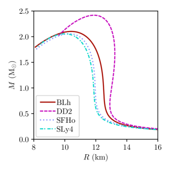
Figure 1: TOV sequences for the EOS models considered in this work.

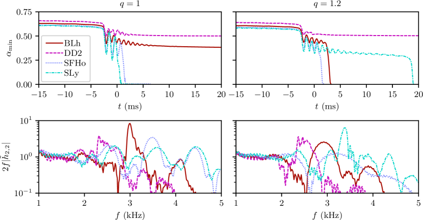
Figure 2: Representative global quantities for the standard resolution (SR) simulations in our work. Top panel: Minimum of the lapse function $\alpha_{\rm min}$ in the case of SR simulations with equal (left panel) and unequal (right panel) mass ratios. Bottom panel: GW spectra for the same simulations depicted in the top panel.

The EOS models we consider consist of the BLh Bombaci and Logoteta (2018), DD2 Hempel and Schaffner-Bielich (2010), SFHo Steiner et al. (2010), and SLy4 Chabanat et al. (1998); Schneider et al. (2017) models. In Fig. 1, we show the sequences of static, non-rotating equilibrium stars (i.e., the Tolman-Oppenheimer-Volkoff (TOV) sequence) corresponding to each EOS considered in this work. We show the TOV sequences for the BLh, DD2, SFHo, and SLy EOSs using the solid maroon, dashed magenta, dotted blue, and dash-dotted cyan lines, respectively. All EOS models produce maximum mass TOV stars with $M_{\rm max}^{\rm TOV}\geq$2\text{\,}\mathrm{M}_{\odot}$$, and as such are consistent with massive pulsar observations Cromartie et al. (2019); Antoniadis et al. (2013, 2016). Several recent, independent methods constrain the radius of a $M=$1.4\text{\,}\mathrm{M}_{\odot}$$ star to $$10\text{\,}\mathrm{k}\mathrm{m}$\lesssim R_{1.4}\lesssim$13\text{\,}\mathrm{k}\mathrm{m}$$, including observations of pulsars in globular clusters Steiner et al. (2018), observations of x-ray pulsars Ozel and Freire (2016); Bogdanov et al. (2019), the GW170817 event Radice and Dai (2019); Christian et al. (2019); Malik et al. (2018); Abbott et al. (2018); Landry and Essick (2019); Carson et al. (2019); Essick et al. (2019); Raithel (2019), and the recent NICER results Raaijmakers et al. (2021); Miller et al. (2021); Riley et al. (2021). All EOS models that we consider obey these constraints on $R_{1.4}$.

We note that all EOS models considered in this work contain strictly hadronic degrees of freedom. EOS models of this type have strong universality properties, and typically exhibit a $\sim 20\%$ increase in the maximum mass when allowing for maximal uniform rotation Breu and Rezzolla (2016), a limit referred to as the ‘supramassive’ mass $M_{\rm supra}$. If the total system mass falls below $M_{\rm supra}$, we expect that the post-merger remnant will not collapse to a BH. With the exception of models which employ EOS DD2, the total system mass for the cases considered in our work falls above $M_{\rm supra}$. Consistent with this picture, all simulations that employ the DD2 EOS do not produce a BH within the end of the simulation. Simulations employing other EOS models may form BHs in the final state, depending on how the postmerger evolution proceeds.

We consider a total of 8 base simulations across the 4 EOS models and 2 different mass ratios. We also consider these simulations at lower grid resolutions and a subset of them at higher grid resolutions, resulting in a total of 20 simulations. We construct initial data using the Lorene spectral solver Gourgoulhon et al. (2016) for BNS systems using cold ($T\approx$0.01\text{\,}\mathrm{M}\mathrm{e}\mathrm{V}$$), $\beta$-equilibrated slices of the EOS models discussed above. Our initial configurations consist of irrotational binaries with initial center-of-mass separations of $45\text{\,}\mathrm{k}\mathrm{m}$. We consider a fixed binary mass of $M=$2.7\text{\,}\mathrm{M}_{\odot}$$ for all cases, and take the mass ratio to be

$$q=M_{1}/M_{2}\geq 1,$$ (11)

where $M_{i}$ is the mass of a TOV star with the same baryonic mass as star $i$ in the binary and the labels $i=1(2)$ correspond to the more (less) massive star in the configuration. In Tab. 1 we list relevant properties for our set of initial data.

III.2 Grid setup

We consider simulations at 2 grid resolutions, which we label low resolution (LR) and standard resolution (SR). The outer boundaries of our grid extend to $\sim\pm$1512\text{\,}\mathrm{k}\mathrm{m}$$ along the $x$- and $y$-directions and to $\sim$1512\text{\,}\mathrm{k}\mathrm{m}$$ along the $z$-direction; we employ reflection symmetry about the $xy$-plane. Our solution grid uses 3 sets of boxes nested within the outermost boundaries with each box employing 7 levels of adaptive mesh refinement (AMR), for which we use the Carpet AMR driver within the EinsteinToolkit Loffler et al. (2012). We place the center of one set of boxes at the origin of the solution grid, near the epicenter of the merger. The two other sets of boxes are used to track the centers-of-mass for each star. The half-side length of the smallest nested boxes extend to $r=$14.8\text{\,}\mathrm{k}\mathrm{m}$$, such that they fully cover the entirety of each NS. The half-side length of the remaining coarser boxes extend to $r=\eta~{}$\mathrm{k}\mathrm{m}$$, where $\eta\in(29.5,59.1,118.2,236.1,443.1)$. The finest-level grid spacing is $\Delta x_{\rm fin}^{\rm LR}\approx$0.25\text{\,}\mathrm{k}\mathrm{m}$$ and $\Delta x_{\rm fin}^{\rm SR}\approx$0.185\text{\,}\mathrm{k}\mathrm{m}$$ for the LR and SR cases, respectively. In Tab. 1 we list the grid resolutions considered for each configuration in our study.

IV Results

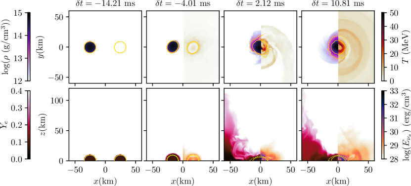
Figure 3: Top panel: Equatorial snapshots of the SR $\text{DD2}_{q=1}$ simulation. We depict the rest mass density $\rho$ on the left half of each panel and the temperature $T$ on the right half of each panel, corresponding to the left and right colorbars, respectively. From left to right, we show snapshots at times from merger $\delta t\equiv t-t_{\rm mer}\in(-14.21,-4.01,2.12,10.81)$\text{\,}\mathrm{m}\mathrm{s}$$. We highlight contours of fixed rest mass densities $\rho=${10}^{13}\text{\,}\mathrm{g}\text{\,}{\mathrm{cm}}^{-3}$$ and $\rho=${10}^{14}\text{\,}\mathrm{g}\text{\,}{\mathrm{cm}}^{-3}$$ using dashed and solid yellow lines, respectively (where $\rho=${10}^{13}\text{\,}\mathrm{g}\text{\,}{\mathrm{cm}}^{-3}$$ is conventionally taken to be the interface between disk and remnant NS). Bottom panel: Meridional snapshots for the same simulation depicted in the top panel. The left and right half of each snapshot depict the electron fraction $Y_{\rm e}$ (corresponding to the left colorbar) and neutrino energy density in the lab frame (corresponding to the right colorbar), respectively.

In the following we highlight the key results from our simulations. We focus on the following results: (A) we detail the general merger dynamics and outcomes, as well as the gravitational radiation extracted from our simulations; (B) we discuss the properties of ejecta; (C) we discuss the general neutrino dynamics and report on neutrino luminosity and energetics; (D) we detail the $r$-process nucleosynthetic yields that arise from our simulations and report on approximate kilonova lightcurves. Where relevant, we highlight how our improved neutrino treatment plays a role on our results.

IV.1 Merger dynamics and gravitational waves

Table 2: Summary of key results from our standard resolution (SR) simulations. For each simulation we list the EOS, mass ratio $q$, approximate time of collapse (after the merger) $\delta t_{\rm coll}$ estimated by the time at which the minimum lapse drops below $\alpha_{\rm min}<0.2$, final simulation time $\delta t_{\rm end}$, and frequency corresponding to peak post-merger GW emission $f_{\rm peak}^{2,2}$. All times are given in ms after the merger.

EOS	$q$	$\delta t_{\rm coll}($\text{\,}\mathrm{m}\mathrm{s}$)$	$\delta t_{\rm end}($\text{\,}\mathrm{m}\mathrm{s}$)$	$f^{2,2}_{\rm peak}($\text{\,}\mathrm{k}\mathrm{H}\mathrm{z}$)$
BLh	1.0	–	21.75	2.99
BLh	1.2	3.29	3.82	2.94
DD2	1.0	–	40.11	2.32
DD2	1.2	–	31.20	2.36
SFHo	1.0	1.76	6.93	3.49
SFHo	1.2	1.87	2.33	3.21
SLy	1.0	0.73	6.09	2.65
SLy	1.2	19.18	19.55	3.38

We begin the discussion of our main results with an overview of the general merger dynamics observed in our simulations. Specifically, we discuss quantities that represent key physics of different stages of the merger, and list some of these quantities in Tab. 2. The merger dynamics observed in our simulations cover three generic scenarios: (1) in some cases we observe relatively short-lived post-merger remnants, with remnant survival times as short as $t\sim$3\text{\,}\mathrm{m}\mathrm{s}$$ as is the case for simulations employing the SFHo EOS; (2) in other cases we observe longer-lived remnants NSs that collapse on timescales closer to $t\sim 20-$30\text{\,}\mathrm{m}\mathrm{s}$$, as is the case for some simulations employing the SLy and BLh EOSs; (3) finally, we find cases which produce post-merger remnants that do not collapse on the timescales covered by our simulations (with survival times exceeding $t\sim$50\text{\,}\mathrm{m}\mathrm{s}$$) as is the case for simulations employing the DD2 EOS. In our simulations we do not observe the prompt-collapse scenario, in which a BH is formed immediately at the time of merger.

In the top panel of Fig. 2 we show the minimum lapse as a function of time for equal (left panel) and unequal (right panel) mass ratios. Fig. 2 reveals that, depending on mass-ratio, different EOS models exemplify scenarios with a short-lived (e.g., $\text{SFHo}_{q=1}$), longer-lived (e.g., $\text{SLy}_{q=1.2}$), and stable post-merger remnant on the timescales probed by our simulations (e.g., $\text{DD2}_{q=1}$ and $\text{DD2}_{q=1.2}$), respectively. In the lower panel of Fig. 2 we show the GW spectrum for our simulations. The inspiral signals are very similar in the amplitude and phase between all cases. Deviations between cases arise mainly in the post-merger stages, where the thermal effects of the EOS are expected to manifest. The high-frequency signal, with $f\geq$2\text{\,}\mathrm{k}\mathrm{H}\mathrm{z}$$, is dominated by the dynamics of the post-merger remnant, with peak frequencies in the range $f_{\rm peak}\approx$2.3\text{\,}\mathrm{k}\mathrm{H}\mathrm{z}$-f_{\rm peak}\approx$3.5\text{\,}\mathrm{k}\mathrm{H}\mathrm{z}$$, depending on the EOS. We find that the mass ratio does not play a strong role in the value of $f_{\rm peak}$, with shifts of at most $\sim 2\%$ across the EOS models considered.

In the top panel Fig. 3 we show equatorial snapshots of the rest mass density $\rho$ and temperature $T$ at different stages of the merger using the left and half right of each panel, respectively. We focus on results for model $\text{DD2}_{q=1}$ at SR. During the inspiral all simulations behave qualitatively similar, with negligible oscillations in $\rho_{\rm max}$ and $\alpha_{\rm min}$ (as suggested by the top panel of Fig. 2) and minimal heating (as suggested by the right half of the two leftmost frames in Fig. 3). The first significant heating happens at a time near merger, when the two stellar cores begin to touch (as depicted in the third-from-left frame in the top panel of Fig. 3 corresponding to $t\approx$2\text{\,}\mathrm{m}\mathrm{s}$$ after the merger). Some simulations produce a longer-lived remnant massive neutron star (RMNS). In these cases, as exemplified by the top right panel of Fig. 3, the RMNS typically develops with a warm core of $T\sim$10\text{\,}\mathrm{M}\mathrm{e}\mathrm{V}$$ which is surrounded by an envelope of hotter material of $T\sim 30-$40\text{\,}\mathrm{M}\mathrm{e}\mathrm{V}$$. This temperature profile is maintained over the lifetime of the remnant as it settles toward an equilibrium state on dynamical timescales.

During the inspiral we find $Y_{\rm e}$ values that reflect the neutron rich conditions consistent with cold neutrino-less beta equilibrium, as expected. After the merger the high density regions comprising the remnant (highlighted with yellow contours in Fig. 3) remain very neutron rich. The disk surrounding the remnant remains neutron rich (with $Y_{\rm e}\lesssim 0.25$) along the orbital plane well after the merger, as depicted in the bottom right panel of Fig. 3. As the angle with the equatorial plane increases, so does the typical $Y_{\rm e}$ value, with the region within approximately $30\deg$ from the polar axis being comprised of proton rich material (with $Y_{\rm e}\geq 0.4$). As discussed in Sec. IV.2, the amount of ejected material with $Y_{\rm e}\geq 0.4$ may be significantly enhanced when M1 neutrino transport is considered, relative to simulations that use lower- order neutrino transport schemes Zappa et al. (2022).

IV.2 Ejecta

Table 3: Summary of key ejecta properties for the SR simulations in our study. For each simulation we list the EOS, mass ratio $q$, time after the merger at which an AH first forms in the simulation $\delta t_{\rm AH}$, total ejected mass $M_{\rm ej,tot}$, ejecta kinetic energy $E_{\rm kin}$ and several mass-averaged quantities, including the asymptotic speed $\langle v_{\infty}\rangle$, electron fraction $\langle Y_{\rm e}\rangle$, specific entropy $\langle s\rangle$, and temperature $\langle T\rangle$. We also show the total amount of “fast” ejecta (with $v_{\infty}\geq 0.6$) $M_{\rm ej}^{v\geq 0.6}$, total amount of “proton-rich” ejecta (with $Y_{\rm e}\geq 0.4$) $M_{\rm ej}^{Y_{\rm e}\geq 0.4}$, and total amount of “shocked” ejecta (with $s\geq 150$ $k_{\rm B}/{\rm baryon}$) $M_{\rm ej}^{s\geq 150}$.

EOS	$q$	$\delta t_{\rm AH}$	$M_{\rm ej,tot}$	$E_{\rm kin}$	$\langle v_{\infty}\rangle$	$\langle Y_{\rm e}\rangle$	$\langle s\rangle$	$\langle T\rangle$	$M_{\rm ej}^{v\geq 0.6}$	$M_{\rm ej}^{Y_{\rm e}\geq 0.4}$	$M_{\rm ej}^{s\geq 150}$
		(ms)	$(10^{-2}M_{\odot})$	$(10^{50}$\text{\,}\mathrm{e}\mathrm{r}\mathrm{g}$)$			$(k_{\rm B}/{\rm baryon})$	(MeV)	$(10^{-2}M_{\odot})$	$(10^{-2}M_{\odot})$	$(10^{-2}M_{\odot})$
BLh	1.0	21.745	0.188	0.605	0.145	0.309	23.747	0.418	$5.949\text{\times}{10}^{-04}\text{\,}$	0.061	$5.603\text{\times}{10}^{-04}\text{\,}$
DD2	1.0	40.096	0.508	0.673	0.079	0.308	19.182	0.509	$3.504\text{\times}{10}^{-08}\text{\,}$	0.144	$2.277\text{\times}{10}^{-04}\text{\,}$
SFHo	1.0	1.762	0.819	6.807	0.287	0.283	16.761	0.697	$1.407\text{\times}{10}^{-02}\text{\,}$	0.017	$9.041\text{\times}{10}^{-04}\text{\,}$
SLy	1.0	0.792	0.342	3.765	0.324	0.230	16.190	0.498	$1.993\text{\times}{10}^{-02}\text{\,}$	0.013	$1.219\text{\times}{10}^{-03}\text{\,}$
DD2	1.2	31.181	0.363	0.530	0.071	0.266	18.494	0.400	$1.069\text{\times}{10}^{-04}\text{\,}$	0.068	$2.220\text{\times}{10}^{-04}\text{\,}$
SLy	1.2	19.179	0.871	3.525	0.152	0.187	13.562	0.327	$8.315\text{\times}{10}^{-03}\text{\,}$	0.101	$8.168\text{\times}{10}^{-04}\text{\,}$

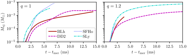
Figure 4: Total ejecta mass for the SR simulations considered in this work. In the left (right) panel we show results for the $q=1$ ($q=1.2$) simulations.

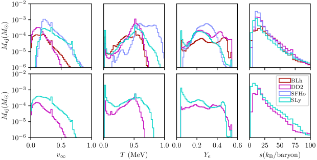
Figure 5: Histograms of ejecta properties for simulations of equal ($q=1$, top panel) and unequal ($q=1.2$, bottom panel) mass ratios. Specifically, we show the total time-averaged ejecta mass for several fluid variables $M_{\rm ej}=\sum_{i}m_{i}$ (where $m_{i}$ is the mass fraction in each variable bin), including the asymptotic velocity $v_{\infty}$, temperature $T$, electron fraction $Y_{\rm e}$, and specific entropy $s$. All results depicted are for SR simulations which produce a significant amount of ejecta.

In Fig. 4 we show the total amount of ejected mass as a function of time for the SR simulations. We find that only some cases result in a significant amount of ejecta due to the duration of the simulations. Specifically, we exclude models $\text{BLh}_{q=1.2}$ and $\text{SFHo}_{q=1.2}$ from the discussion on ejecta because we could not carry out the simulations to sufficiently late times.

In Tab. 3 we summarize the key average ejecta properties pertaining to the subset of models which produce significant ejecta. For cases with $q=1$ ($q=1.2$), models $\text{SFHo}_{q=1}$ ($\text{SLy}_{q=1.2}$) produce the most ejecta, with both cases producing close to $0.01\text{\,}\mathrm{M}_{\odot}$. We note qualitative trends in the mass-averaged ejecta properties that potentially reflect the main effects of the EOS and the use of M1 neutrino transport. For instance, we note that the ‘stiffer’ EOSs we consider (namely, models BLh and DD2) produce ejecta with higher $\langle Y_{\rm e}\rangle$, but lower $\langle v_{\infty}\rangle$. Qualitatively, stiffer EOS models (such as BLH and DD2) allow for higher maximum remnant masses and lead to longer remnant lifetimes Margalit and Metzger (2017); the production of metastable RMNSs which survive on significantly longer timescales for stiffer EOS models is demonstrated by the $\delta t_{\rm AH}$ quantity in Tab. 3. On the other hand, ‘softer’ EOS models such as SFHo and SLy result in more compact binary components that undergo more violent collisions at the merger and produce stronger shocks Radice et al. (2018a). The aforementioned trends we observe in $\langle Y_{\rm e}\rangle$ and $\langle v_{\infty}\rangle$ may be attributed to the combined effects of the EOS and M1 neutrino transport. Where ‘softer’ EOS models lead to more violent shocks at the time of merger and produce higher velocity shocked ejecta, the relatively low maximum remnant masses they allow for result in significantly shorter neutrino irradiation times in the post-merger which in turn allows the disk surrounding the remnant to remain relatively neutron rich. On the other hand, ‘stiffer’ EOS models may produce lower velocity shocked ejecta while allowing for longer-lived RMNSs that irradiate the disk with neutrinos and drive the electron fraction in the system toward higher values Zappa et al. (2022).

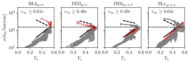
Figure 6: Relation between the mass-and-azimuthally-averaged specific entropy $s$ and electron fraction $Y_{\rm e}$ for ejecta in four representative SR simulations in our work. We highlight the ejecta with asymptotic velocity $v_{\infty}$ that falls above the $99^{\rm th}$ percentile of the distribution (with value shown in each panel) using red marks. For reference, we also show approximate fits for potentially disparate components of the ejecta using dashed and solid black lines, and mark the the threshold above which we could potentially mark shocked ejecta ($s\geq 150\text{ }k_{\rm B}/{\rm baryon}$) with a black dotted line.

In Fig. 5 we show histograms of relevant ejecta properties for SR simulations which produce a significant amount of ejecta. In Zappa et al. (2022) it was found that the M0 and M1 schemes as implemented in the THC code result in qualitatively similar ejecta. The main difference between the predictions of each scheme, in the context of ejecta, is reflected in the electron fraction distribution. Specifically, when compared to M0 cases, simulations employing the M1 scheme may produce significantly more proton-rich ejecta. This is reflected in the ejecta distribution of $Y_{\rm e}$ for the simulations presented in Fig. 5. In particular, the distributions corresponding to models $\text{BLh}_{q=1}$, $\text{DD2}_{q=1}$, $\text{DD2}_{q=1.2}$, and $\text{SLy}_{q=1}$ simulations exhibit a significant amount of high-$Y_{\rm e}$ ejecta (with $Y_{\rm e}\geq 0.4$). The relative increase of high-$Y_{\rm e}$ ejecta in M1 simulations is attributed to the “protonization” of ejecta fluid elements which absorb neutrinos that originate in the central object and disk Zappa et al. (2022); neutrino absorption in the ejecta leads to a systematic increase of the electron fraction. We note that the aforementioned models all produce metastable RMNSs that survive until the end of the simulation, which is consistent with the picture of longer-lived RMNSs as neutrino sources that produce significant proton-rich material.

Ejecta profiles extracted from BNS merger simulations may suggest the existence of correlations between certain ejecta properties Nedora et al. (2020); Camilletti et al. (2022). Of particular interest is the fast ejecta, which may constitute a dense environment through which the jet needs to breakout to power prompt GRB emission Beloborodov et al. (2020), may potentially produce non-thermal emission as it shocks the interstellar medium Nakar and Piran (2011), may power a short (${\sim}1$ hour) UV transient due to free neutrons decay Metzger et al. (2015); Combi and Siegel (2023a, b), and may be the origin of the late-time X-ray excess associated with GW170817 Hajela et al. (2022); Nedora et al. (2021b). If indeed strong correlations exist between particular properties of the fast ejecta, this may inform modeling efforts targeted at explaining the aforementioned phenomena Bauswein et al. (2013b); Ishii et al. (2018); Radice et al. (2018a); Dean et al. (2021). In the left panel of Fig. 5 we show histograms for the asymptotic velocity $v_{\infty}$. High speed ejecta are expected to be produced in the violent shocks that arise during the merger Nedora et al. (2020). The neutrino scheme employed is not expected to play a significant role in determining the amount of fast ejecta Zappa et al. (2022), so we instead focus on the effects of the EOS when discussing the properties of fast ejecta. The increased amount of fast ejecta in simulations with relatively soft EOSs (e.g., SFHo and SLy) is consistent with the picture that such EOS models result in relatively compact binary components which undergo relatively violent mergers and in turn produce higher velocity ejecta Nedora et al. (2021b) (see Tab. 3 for reference, where we show the amount of ejecta with $v_{\infty}\geq 0.6$). We note that variability in the amount of fast ejecta which is reflected by the tails of the $\langle v_{\infty}\rangle$ the histograms in Fig. 5. For instance, focusing on the top panel of Fig. 5, models $\text{BLh}_{q=1}$ and $\text{DD2}_{q=1}$ show very few ejecta with $v_{\infty}\geq 0.45$ and $v_{\infty}\geq 0.6$, respectively. On the other hand, models $\text{SFHo}_{q=1}$ and $\text{SLy}_{q=1}$ show a significant amount of ejecta with $v_{\infty}\geq 0.6$.

We focus on the relationship between the mass-and-azimuthally-averaged specific entropy and electron fraction as an example of quantities that show a potential correlation, which we show in Fig. 6 for a representative subset of our simulations. In Fig. 6 we highlight the component of the ejecta which falls above the $99^{\rm th}$ percentile in asymptotic speed (for clarity we show the value of this speed as labels in Fig. 6) using red markers and show the remainder of the ejecta in gray. We also show approximate fits for two potentially disparate components of the ejecta using solid and dashed black lines. We find that, depending on the EOS and mass ratio, it may be possible to identify disparate components of the ejecta based on whether it is fast or not. For example, for models $\text{BLh}_{q=1}$ and $\text{DD2}_{q=1}$ we find that using the aforementioned criterion to label fast ejecta results in a unique anti-correlation between $s$ and $Y_{\rm e}$ which closely follows the approximate fit represented by the dashed line (as shown in the leftmost panel of Fig. 6), whereas the remainder of the ejecta approximately follows the trend highlighted by the solid black line. However, the trend reflected in the fast ejecta for models $\text{BLh}_{q=1}$ and $\text{DD2}_{q=1}$ is not robust across different mass ratios or EOS models. For example, the results for models $\text{DD2}_{q=1.2}$ and $\text{SLy}_{q=1.2}$ show that we cannot isolate the fast ejecta as following a different trend than the remainder of the ejecta. We have additionally considered a fixed criterion of $v_{\infty}\geq 0.6$ to label the fast ejecta, but this leads to even higher variability in the potential correlations depicted in Fig. 6 across different EOS models and mass ratios.

We note that for all simulations considered here it may be possible to identify a separate component based instead on the specific entropy. It is clear from Fig. 6 that the component of ejecta with $s\gtrsim 150$ $k_{\rm B}/{\rm baryon}$ (highlighted by the horizontal black dotted line in Fig. 6) shows an anti-correlation between $s$ and $Y_{\rm e}$ for all models. The source of this component of the ejecta is likely shocks that develop during the merger and shortly after, as this is the source of the highest entropy and temperature material we observe. The aforementioned relations may also be due to the absorption of neutrinos (or lack thereof) for different components of the ejecta. For instance, the very fastest ejecta may become diluted before absorbing many neutrinos and as such does not have its $Y_{\rm e}$ increased by neutrino absorption. Since $v_{\infty}\propto s$ for shocked ejecta (as is the case for models $\text{BLh}_{q=1}$ and $\text{DD2}_{q=1}$), we may find that $s$ and $Y_{\rm e}$ are anti-correlated for this component. On the other hand, the slower ejecta may have both $Y_{\rm e}$ and $s$ increased by absorption, and may end up with $Y_{\rm e}\propto s$ (which may be similar to what occurs with neutrino driven winds Nedora et al. (2021c)). We emphasize that the total amount of ejecta with $s\gtrsim 150$ $k_{\rm B}/{\rm baryon}$ is very small as shown in Tab. 3 (typically $10^{-6}-${10}^{-5}\text{\,}\mathrm{M}_{\odot}$$). Aside from the relations depicted in Fig. 6, we have also considered potential correlations among other relevant ejecta properties such as between temperature $T$, rest mass density $\rho$, and flux $F$. Besides those discussed above, we find no additional evidence of trends or correlations in the properties of fast or shocked ejecta which are robust across EOS models and mass ratios. Correlations in the properties of fast ejecta, if they exist, may require higher accuracy numerical methods to reliably capture and are potentially sensitive to the grid resolution and numerical methods used Bauswein et al. (2013b); Ishii et al. (2018); Radice et al. (2018a); Dean et al. (2021).

IV.3 Neutrino luminosity

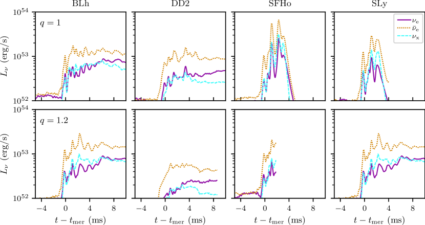
Figure 7: Neutrino luminosity for the SR simulations in our work. We show results for the equal and unequal mass ratio cases in the top and bottom panels, respectively.

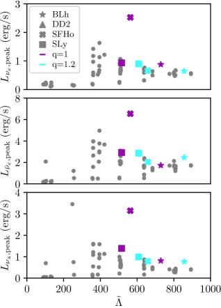
Figure 8: Peak neutrino luminosity as a function of reduced tidal deformability for the SR simulations in this work. Equal (unequal) mass ratio results are shown in purple (cyan). For reference, we show the same quantity for the M0 simulations considered in Cusinato et al. (2021) using gray dots.

The key new feature in the simulations presented in this work is the use of M1 neutrino transport, which we briefly reviewed in Sec. 8. In this Section we highlight the main neutrino microphysics effects observed in our simulations, including the peak neutrino luminosities predicted by our simulations, the production of neutrinos during different stages of the merger, and a comparison between the neutrino and GW luminosity. Where relevant, we compare our findings to current results in the literature which use alternative neutrino transport schemes.

Our simulations show that neutrino production during the inspiral is negligible in high-density regions. As suggested by the third frame, top panel in Fig. 3, the first significant shock heating happens at the point of first-contact between the binary components, at a time close to $t_{\rm mer}$. Similarly, we find that the peak neutrino energy density is reached close to this time (as depicted by the third frame, bottom panel in Fig. 3). In Fig. 7 we show the neutrino luminosity $L_{\nu}$ as a function of time for the SR simulations considered in this work. The peak neutrino luminosity is typically reached within $4\text{\,}\mathrm{m}\mathrm{s}$ of the merger. We generally find neutrino dynamics and energetics which are compatible with findings from throughout the literature and which use alternative neutrino transport schemes. For instance, we find general agreement between the peak neutrino luminosity and energies predicted by the M1 simulations considered in this work and those which use a lower-order M0 neutrino treatment Cusinato et al. (2021) as well as those which employ an MC scheme Foucart et al. (2022b) (with peak luminosities on the order of ${10}^{53}\text{\,}\mathrm{e}\mathrm{r}\mathrm{g}\mathrm{/}\mathrm{s}$). Moreover, in all simulations we find that the neutrino species follow the same order in brightness, with the species corresponding to heavy-lepton flavors $\nu_{\rm x}$ being the dimmest, followed by the electron neutrino $\nu_{\rm e}$ and finally the electron anti-neutrino $\bar{\nu}_{\rm e}$ being the brightest. The general qualitative agreement between simulations employing the lower order M0 scheme and the simulations presented in this work is encouraging and may be a sign of the early convergence of moment based schemes. We refer the reader to Zappa et al. (2022) for deeper comparisons between the results of the M0 and M1 schemes as implemented in the THC code.

In Fig. 8 we show the peak neutrino luminosity as functions of the tidal deformability of the binary for the SR simulations in this work. The reduced tidal deformability is defined as Favata et al. (2004)

$$\tilde{\Lambda}\equiv\dfrac{16}{13}\left[\dfrac{(M_{1}+12M_{2})M_{1}^{4}}{(M_{1}+M_{2})^{5}}\Lambda_{1}+(1\leftrightarrow 2)\right],$$ (12)

where we use the same labeling convention as in Eq. (11) and the tidal deformability of each binary component is $\Lambda_{i}=2\kappa_{2}R_{i}^{5}/(3M_{i}^{5})$, where $\kappa_{2}$ is the quadrupolar Love number. In Fig. 8 we also depict results for the M0 simulations considered in Cusinato et al. (2021) for reference. Similar to the trend highlighted in Cusinato et al. (2021) for M0 simulations, we note an apparent anti-correlation between the peak neutrino luminosity and reduced tidal deformability. The tidal deformability of the system increases as the binary components become less compact. As such, the merger of systems with larger tidal deformability is relatively less violent and results in weaker shock heating of the material during merger. As the shocks produced during the merger are key sites for neutrino production (see Fig. 3 for reference), less violent shocks result in lower neutrino luminosities. We note that model $\text{SFHo}_{q=1}$ results in significantly higher luminosities than all other cases considered, as shown in the top panel of Fig. 7, which results in the model appearing as an outlier in the trends depicted in Fig. 8. Nevertheless, the remainder of the models we consider show strong support for the anti-correlation between the peak neutrino luminosity and tidal deformability as originally pointed out in Cusinato et al. (2021).

In Fig. 9 we also show the peak neutrino luminosity as a function of the peak GW luminosity for the same models considered in Fig. 8. The relationship between peak neutrino and GW luminosities originally discussed in Cusinato et al. (2021) allows for the identification of two potential groups of models, depending on the lifetime of the RMNS formed after the merger. Firstly, for models that promptly collapse to a BH at the time of merger, the peak neutrino luminosity may be weakly anti-correlated with the peak GW luminosity; these models mostly reside within the yellow shaded region in Fig. 9. Secondly, for models that form RMNSs, the peak neutrino and GW luminosities may be correlated; these models mostly reside within the red shaded region in Fig. 9. In the case of the trends depicted in Fig. 9 we note that most models considered in this work fall within the group of models that show a correlation between $L_{{\rm peak},\nu_{\rm tot}}$ and $L_{{\rm peak,GW}}$ (i.e., within the red shaded region in Fig. 9). Similar to the potential mechanism behind the trends depicted in Fig. 8, the more violent shocks produced during mergers with higher peak GW luminosity results in higher neutrino peak luminosities. We note that all cases considered in our study produce a RMNS, albeit with different lifetimes. Variability in the correlation between the peak neutrino and GW luminosities may be related to the lifetime of the RMNS Cusinato et al. (2021), with short-lived remnants that collapse within $5\text{\,}\mathrm{m}\mathrm{s}$ after the merger tending to produce higher neutrino and GW luminosities indicative of more violent mergers. However, we find that for the M1 simulations considered in our work it is not straightforward to cleanly divide models which produce remnants that survive for longer than $5\text{\,}\mathrm{m}\mathrm{s}$ after the merger from those that do not. For instance, models $\text{SFHo}_{q=1}$ and $\text{BLh}_{q=1}$ produce very similar neutrino and GW luminosities, despite producing RMNSs that survive for approximately only $2\text{\,}\mathrm{m}\mathrm{s}$ and over $40\text{\,}\mathrm{m}\mathrm{s}$, respectively. We also note that model $\text{SFHo}_{q=1}$, which stands out as a potential outlier in the trends depicted in Fig. 8, also stands out as a potential outlier in the trends depicted in Fig. 9 along with one other model which employed M0 neutrino transport.

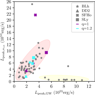
Figure 9: Peak neutrino luminosity $L_{{\rm peak},\nu_{\rm tot}}$ as a function of peak GW luminosity $L_{\rm peak,GW}$ for the SR simulations in our work. Equal (unequal) mass ratio results are shown in purple (cyan). For reference we show the same quantity for the M0 simulations considered in Cusinato et al. (2021) using gray dots. We highlight potential distinct groups of models based on the lifetime of the RMNS produced after the merger; with the yellow and red shaded regions roughly corresponding to models that promptly form BHs and models that form RMNSs, respectively.

IV.4 Nucleosynthesis and kilonova signals

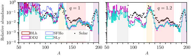
Figure 10: Relative abundance of $r$-process elements calculated using average ejecta properties extracted from our simulations. We normalize such that all models produce the same total abundance for elements with atomic number $A\geq 170$, which results in similar amounts of third-peak $r$-process elements in all cases (highlighted using the rightmost shaded region). We focus on 4 representative models and show the resulting nucleosynthesis abundance using color lines. For reference, we show the relative abundance for Solar elements with black dots, using the same normalization.

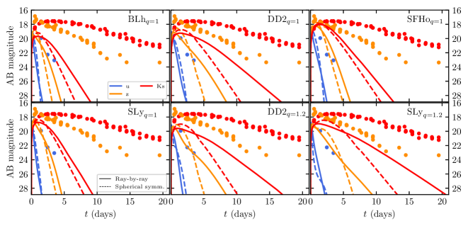
Figure 11: Absolute bolometric (AB) magnitude associated with synthetic kilonova lightcurves for 6 representative models. We show three representative bands using different color lines. We compare synthetic light curves computed by assuming spherical symmetry (dashed lines) to light curves computed by assuming axisymmetry (solid lines) with a ray-by-ray procedure. For reference, we also show the magnitudes measured for AT2017gfo  Chornock et al. (2017); Cowperthwaite et al. (2017) using dots.

As discussed in Sec. IV.2, a key effect of M1 neutrino transport is the capture of neutrino absorption which may lead to the significant protonization of ejecta (i.e., a significant increase in the amount of ejected matter with $Y_{\rm e}\geq 0.4$); this effect is most pronounced when comparing the ejecta distributions in $Y_{\rm e}$, as shown in Fig. 5, between simulations that lead to longer-lived RMNSs and those that do not. In Fig. 10 we show the relative abundance of elements predicted by several SR simulations in our work, along with solar abundances for reference (we also highlight the regions roughly corresponding to the first, second, lanthanide, and third $r$-process peaks using gray, orange, red, and purple bands, respectively). We normalize all abundances such that the total amount of material above $A=170$ is equivalent among models, which results in similar abundances in the third $r$-process peak elements. All models considered produce second and third peak abundances which are consistent with the solar pattern. Among the set of models depicted in Fig. 10 we consider cases which result in both short and longer-lived RMNSs. Although these differences in post-merger evolution are reflected in the $Y_{\rm e}$ distribution of the ejecta, they do not appear to significantly affect the nucleosynthetic yield of $r$-process elements. For instance, all models predict similar abundances for the second, third, and lanthanide peaks despite significantly different remnant lifetimes and neutrino irradiation times. Moreover, models $\text{SFHo}_{q=1}$ and $\text{SLy}_{q=1}$ (which result in short-lived RMNSs) predict larger and smaller first-peak abundances, respectively, when compared to models that result in longer-lived RMNS. In brief, we do not find clear trends or correlations between the nucleosynthesis yields and the RMNS lifetime (and thereby neutrino irradiation time).

A potential trend which we do note is between the mass-and-time-averaged ejecta temperature (at a fixed radius from the source) and the abundance of elements between the first and second $r$-process peaks (i.e., with $90\lesssim A\lesssim 120$). For instance, we note that model $\text{SFHo}_{q=1}$ ($\text{SLy}_{q=1.2}$) produces the largest (smallest) relative abundance of elements between the first and second peaks. All other models roughly follow a trend that suggests the larger $\langle T\rangle$, the larger the relative abundance of elements with $90\lesssim A\lesssim 120$. In Fig. 12 we show the total relative abundance of elements with $90\leq A\leq 120$ (in other words, the sum of the relative abundances depicted in Fig. 10 with $90\leq A\leq 120$) for each model depicted in Fig. 10. We see a clear correlation between the relative abundance of elements with $90\leq A\leq 120$ and $\langle T\rangle$. We note that the typical temperatures of the ejecta for the models we consider is close to the threshold for nuclear statistical equilibrium (NSE) freeze-out of $T\approx$5\text{\,}\mathrm{G}\mathrm{K}$\approx$0.4\text{\,}\mathrm{M}\mathrm{e}\mathrm{V}$$, above which the temperature-sensitive photo-disintegration reaction cross-sections (which are important in determining the abundance of elements with with $90\lesssim A\lesssim 120$) are expected to be large Perego et al. (2021). The sensitivity of the abundance of elements with $90\lesssim A\lesssim 120$ to the average ejecta temperature may be reflective of the sensitivity of the photo-disintegration cross-section to temperature. We emphasize that $\langle T\rangle$ is the average temperature at a fixed radius, and that the temperature is expected to change as the ejecta expands. An additional potential caveat of the preceding discussion is that ejecta properties may depend sensitively on the grid resolution considered (see App. A for additional detail). Nevertheless, it is interesting to note potential correlations between average ejecta properties such as $\langle T\rangle$ and the nucleosynthetic patterns. We leave an investigation of the robustness of the potential correlation between $\langle T\rangle$ and the abundance of elements with $90\lesssim A\lesssim 120$, along with other potential trends, to future work.

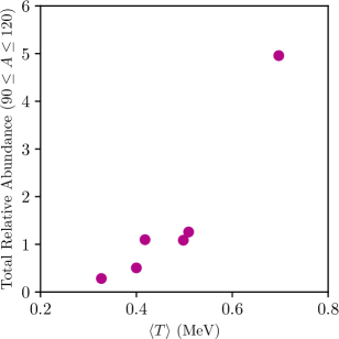
Figure 12: Total abundance of nucleosynthetic yield (relative to the abundance of elements with $A\geq 170$, which we normalize for all models) for elements with $90\leq A\leq 120$ as a function of mass-and-time-averaged ejecta temperature (at a fixed radius). Each datum corresponds to a single SR simulation from our work.

In Fig. 11 we show the absolute bolometric (AB) magnitudes for kilonova signals associated with a subset of simulations in our work; for reference we also show the AB magnitude for the KN signal AT2017gfo. We compute light curves in two ways: assuming spherical symmetry and assuming axisymmetry. In the latter case ray-by-ray independent evolutions are performed for a discrete number of polar angles and the results obtained for each angle are then combined together to obtain the total AB magnitude. We again focus on a subset of representative models to understand the effects of the EOS and the mass ratio.

We generally find KN lightcurves which are significantly dimmer than AT2017gfo data. However, discrepancies between the predicted lightcurves of BNS merger simulations and the AT2017gfo observation are expected and may be due to the relatively short duration simulations we consider which do not account for matter ejected on secular timescales or uncertainties stemming from multidimensional effects and viewing angle Perego et al. (2017b). Moreover, we did not target the simulations in this work to reproduce the system associated with AT2017gfo. As such, we focus the remainder of the discussion around KN on the component produced by the dynamical ejecta.

We find that all models result in similar dynamical ejecta KN lightcurves, typically peaking between 1-2 days in all bands. We note that the KN for models $\text{SLy}_{q=1}$ and $\text{BLh}_{q=1}$ (which produce the shortest and one of the longest lifetime RMNSs, respectively) both decay within approximately 7 days. By comparison, models $\text{DD2}_{q=1}$ and $\text{SFHo}_{q=1}$ result in lightcurves which decay after roughly 10 days, despite the significant differences in RMNS lifetime between those cases. Such differences in KN lightcurves may not be attributable to the enhanced neutrino absorption introduced by the M1 scheme, but rather to differences in the total amount of ejecta that each model produces. With reference to Tab. 3, we note that models which produce fewer ejecta lead to shorter-duration KN. For example, model $\text{BLh}_{q=1}$ ($\text{SLy}_{q=1.2}$) produces the least (most) amount of total ejecta and decays the fastest (slowest). The total amount of ejecta may be sensitive to effects such as the numerical grid resolution as we discuss in App. A, but is not significantly affected by the use of the M1 scheme over the M0 scheme Zappa et al. (2022). All cases considered result in KN lightcurves consistent with a dynamical component which becomes transparent within a few days. Specifically, models $\text{BLh}_{q=1}$, $\text{DD2}_{q=1}$, $\text{SFHo}_{q=1}$, $\text{SLy}_{q=1}$, $\text{BLh}_{q=1.2}$, and $\text{SLy}_{q=1.2}$ result in dynamical ejecta which becomes transparent after roughly 1.6, 3.9, 2.5, 2.4, 4.1, and 7.4 days, respectively. This pattern roughly follows the evolution time of the KN for each model, with models $\text{BLh}_{q=1}$ ($\text{SLy}_{q=1.2}$) resulting in the shortest (longest) time to transparency and slowest (fastest) KN evolution and all other cases resulting in comparable time to transparency and evolution times. We note a general improvement in the light curves calculated with the ray-by-ray procedure. Despite the peak of the light curves in this case not being brighter than the ones calculated in spherical symmetry, their decay at later times ($\gtrsim 5$ days after the merger) follows the experimental data more closely. This is particularly evident focusing on the Ks band for the models simulated with the DD2 EOS, for which we recover an AB magnitude of ${\sim}24$ at 10 days after merger with KNEC computations in axisymmetry, against ${\sim}28$ found with KNEC spherical symmetric evolutions. We expect a further improvement of these results in long-term simulations with a delayed BH collapse Zappa et al. (2022), which include large amount of spiral-wave winds Nedora et al. (2019) and disk winds ejected at secular timescales.

V Conclusion

In this work we have presented an investigation of the combined effects of M1 neutrino transport, the EOS model, and the mass ratio in 3D GRHD BNS merger simulations. The state-of-the-art simulations presented in this work elucidate the role of accurate neutrino transport. We find general agreement between the predicted neutrino luminosities in M0 Zappa et al. (2022), M1 Zappa et al. (2022), and MC simulations Foucart et al. (2022b), and note that M1 simulations appear to support the potential trends between peak neutrino and GW luminosities discussed in Cusinato et al. (2021). Although we find general qualitative agreement between the simulations presented in this work and those that consider alternative neutrino transport schemes such as M0 or MC, we find that there are quantitative differences in the prediction of several effects.

Regarding ejecta properties, we find that the effects of the EOS and the enhanced neutrino absorption introduced by the use of the M1 scheme can conspire to give qualitatively different outcomes to what is typically observed using lower-accuracy methods such as M0 neutrino transport. Along with the details of the viscosity model used (which was left fixed for all simulations in this work), the EOS largely determines the longevity of the metastable RMNS produced during BNS merger simulations Margalit and Metzger (2017). Different RMNS lifetimes can in turn significantly impact the neutrino irradiation time, as the main source of neutrino radiation in the post-merger stage is the RMNS. When accounting for the accurate neutrino re-absorption captured by the M1 scheme, differences in the neutrino irradiation time result in significant differences in the average electron fraction of the system. Specifically, simulations that produce longer-lived RMNSs lead to relatively high average electron fractions when compared to simulations that result in short-lived RMNSs, reflective of the protonization effect introduced by neutrino absorption. The amount of high $Y_{\rm e}$ ejecta (with $Y_{\rm e}\geq 0.4$) is typically a factor of 6-10 times larger (see Tab. 3 for reference) in simulations that produce RMNSs that survive over the duration of the simulations (typically at least $15\text{\,}\mathrm{m}\mathrm{s}$ post-merger). Such differences in the amount of high $Y_{\rm e}$ material is not reliably captured by lower accuracy neutrino transport schemes Zappa et al. (2022), and appears to be a novel feature captured by the M1 simulations presented here. We find that the use of an M1 scheme does not significantly impact the amount of shocked fast ejecta produced during the merger. We note that it may be possible to identify disparate components of the ejecta based on the asymptotic speed (see Fig. 6 for reference). However, these trends are not robust across different EOS models or mass ratios. Interestingly, across our simulations it is possible to separate different components of the ejecta based on the entropy. In particular high-entropy ejecta, likely stemming from the production of shocks, appears to show an anti-correlation between the specific entropy and electron fraction.

We find that the nucleosynthesis pattern does not reflect the aforementioned enhancement of high $Y_{\rm e}$ material introduced by the M1 scheme, and is potentially more sensitive to the the average ejecta temperature $\langle T\rangle$. Specifically, we note a potential correlation between the relative abundance of elements with $90\lesssim A\lesssim 120$ and $\langle T\rangle$. Finally, we note that all models considered lead to qualitatively similar synthetic KN lightcurves consistent with dynamical ejecta, while showing variation in the evolution time and time at which the ejecta become transparent. The decay time of the synthetic KN lightcurves we calculate appear to be sensitive to the total amount of ejecta produced by each model, which is not strongly affected by the neutrino transport scheme Zappa et al. (2022).

In this work we have presented several key BNS merger phenomena where accurate neutrino transport may play a role. Our aim was to consider a wide variety of phenomena which could be impacted by the neutrino transport scheme. The results presented in this work leave open many avenues of investigation. For example, future work may consider the robustness of the effect of M1 neutrino transport in producing enhanced amounts of high-$Y_{\rm e}$ materials for cases that produce longer-lived RMNSs, by considering considerably longer post merger evolutions. In particular, it would be interesting to consider whether the enhanced protonization of the medium introduced by the M1 scheme continues long after the merger, or if there is a limit to the amount of high-$Y_{\rm e}$ ejecta produced. Taking advantage of the reliable neutrino absorption capture by the M1 scheme, it would also be interesting to quantify the size and nature of emergent bulk viscosity from out-of-equilibrium dynamics Espino et al. (2023). We leave a full investigation of the effects of M1 neutrino transport on longer-lived RMNS environments and a calculation of the bulk viscosity which arises during BNS mergers, with M1 neutrino transport, to future work.

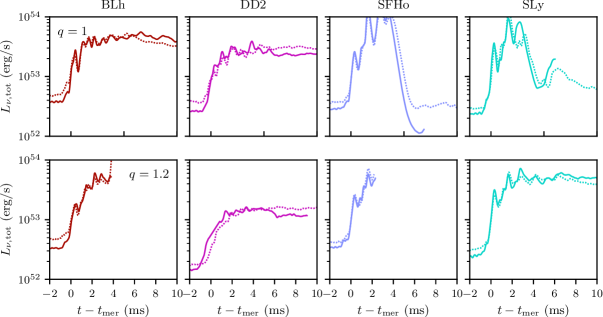
Figure 13: Total neutrino luminosity for the LR (dotted lines) and SR (solid lines) simulations in our work. The top and bottom panel show results for the equal and unequal mass ratio simulations, respectively.

Appendix A On the potential effects of grid resolution

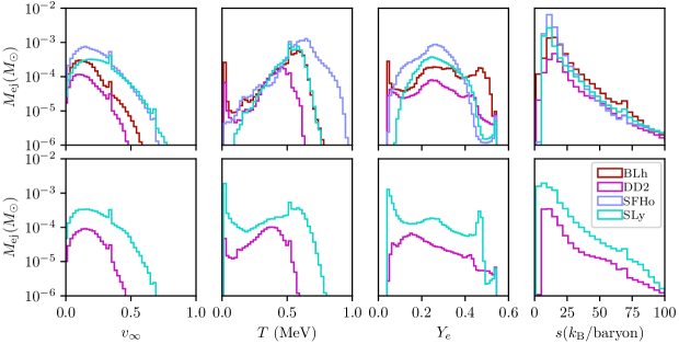
Figure 14: Histograms of ejecta properties for LR simulations of equal ($q=1$, top panel) and unequal ($q=1.2$, bottom panel) mass ratios. We depict histograms for several fluid variables, including the asymptotic velocity $v_{\infty}$, temperature $T$, electron fraction $Y_{\rm e}$, and specific entropy $s$. We show results corresponding to the BLh, DD2, SFHo, and SLy EOS models using solid maroon, dashed magenta, blue, and green lines, respectively.

Table 4: Summary of key ejecta properties for the LR simulations in our study. We list the same quantities considered in Tab. 3. Additionally, in the rightmost column we show the absolute difference in total ejecta mass between the SR and LR cases $\delta M_{\rm ej}\equiv M_{\rm ej,tot}^{\rm SR}-M_{\rm ej,tot}^{\rm LR}$, accounting for differences in total simulation time.

EOS	$q$	$\delta t_{\rm AH}$	$M_{\rm ej,tot}$	$E_{\rm kin}$	$\langle v_{\infty}\rangle$	$\langle Y_{\rm e}\rangle$	$\langle s\rangle$	$\langle T\rangle$	$M_{\rm ej}^{v\geq 0.6}$	$M_{\rm ej}^{Y_{\rm e}\geq 0.4}$	$M_{\rm ej}^{s\geq 150}$	$\delta M_{\rm ej}$
		(ms)	$(10^{-2}M_{\odot})$	$(10^{50}$\text{\,}\mathrm{e}\mathrm{r}\mathrm{g}$)$			$(k_{\rm B}/{\rm baryon})$	(MeV)	$(10^{-2}M_{\odot})$	$(10^{-2}M_{\odot})$	$(10^{-2}M_{\odot})$	$(10^{-2}M_{\odot})$
BLh	1.0	26.054	0.542	0.941	0.090	0.298	19.650	0.496	$1.454\text{\times}{10}^{-04}\text{\,}$	0.140	$4.718\text{\times}{10}^{-04}\text{\,}$	0.185
DD2	1.0	13.539	0.166	0.336	0.110	0.259	21.274	0.402	$0.000\text{\times}{10}^{00}\text{\,}$	0.021	$1.682\text{\times}{10}^{-04}\text{\,}$	0.066
SFHo	1.0	2.033	1.294	5.027	0.158	0.252	14.565	0.610	$5.342\text{\times}{10}^{-03}\text{\,}$	0.016	$1.307\text{\times}{10}^{-03}\text{\,}$	0.019
SLy	1.0	1.072	0.609	3.723	0.215	0.272	15.398	0.529	$7.713\text{\times}{10}^{-03}\text{\,}$	0.032	$9.772\text{\times}{10}^{-04}\text{\,}$	-0.120
DD2	1.2	10.639	0.126	0.327	0.136	0.224	18.579	0.325	$0.000\text{\times}{10}^{00}\text{\,}$	0.012	$1.403\text{\times}{10}^{-04}\text{\,}$	-0.017
SLy	1.2	20.679	0.789	2.959	0.144	0.189	14.432	0.322	$2.620\text{\times}{10}^{-03}\text{\,}$	0.095	$7.820\text{\times}{10}^{-04}\text{\,}$	-0.106

In order to understand the effects of grid resolution on our results, we consider a subset of simulations in our study at different grid resolutions. Specifically, we consider all models with lower resolution grids. Recently, extensive resolution studies of the THC_M1 code have been carried out in  Radice et al. (2022) and Zappa et al. (2022), and we refer the reader to those works for a clearer understanding of the effects of resolution. Here we focus on the effects of resolution on the key microphysics quantities considered in Sec. IV, with particular focus on the neutrino luminosities and ejecta properties.

In Fig. 13 we show the total neutrino luminosity for the LR and SR simulations in our work. We find similar luminosities at both grid resolutions, with the LR simulations predicting slightly higher (by typically 20%) luminosities prior to the merger but very similar (with relative difference of at most 10%) after the merger. We also find that the order of brightness between neutrino species is the same for LR and SR simulations, and is consistent with findings using M0 Cusinato et al. (2021) and MC Foucart et al. (2022b) neutrino transport. This suggests that uncertainties associated with low grid resolutions are as important as uncertainties associated with using approximate neutrino transport schemes, and as such low-resolution results using full neutrino transport schemes may not be reliable for the calibration of approximate methods.

In Fig. 14 we show histograms for the LR simulations of the ejecta mass in the relevant quantities discussed in Sec. IV.2. We find that the protonization effect introduced by enhances neutrino irradiation by the RMNS in the M1 scheme is not captured to the same extent in the LR simulations as it is in the SR simulations. Although we do see a relative increase in the amount of ejecta with $Y_{\rm e}\geq 0.4$ for LR simulations, the enhancement is not as large as we observe for the SR simulations discussed in Sec. IV.2. The highest relative increase in the amount of high-$Y_{\rm e}$ (with $Y_{\rm e}\geq 0.4$) ejecta when comparing SR simulations with a longer-lived RMNS to those with short-lived RMNS is approximately a factor of 12 (specifically when comparing the SR $\text{DD2}_{q=1}$ and $\text{SFHo}_{q=1}$ models). On the other hand, the highest relative increase we observe for LR simulations is approximately only a factor of 9 (when comparing the analogous LR models the LR $\text{BLh}_{q=1}$ and $\text{SFHo}_{q=1}$ models). This potential effect of the grid resolution is mostly reflected when comparing the LR and SR simulations for model $\text{DD2}_{q=1}$, which predict $0.021\text{\times}{10}^{-2}\text{\,}\mathrm{M}_{\odot}$ and $0.144\text{\times}{10}^{-2}\text{\,}\mathrm{M}_{\odot}$ of high-$Y_{\rm e}$ material, respectively. The relatively lower amounts of high-$Y_{\rm e}$ material for the LR simulations considered in our work may also be conflated by having a different duration for each simulation. It may be the case that the longer the RMNS is present, the higher the extent of protonization and deposition of lepton number in the ejecta. We leave a full investigation of the combined effects of the RMNS lifetime and the extent of protonization of the ejecta capture by M1 neutrino transport to future work.

In Tab. 4 we also show global and average ejecta properties for the LR simulations in our work. For reference, we also show the absolute difference in the total ejecta mass predicted by each simulation, $\delta M_{\rm ej}\equiv M_{\rm ej,tot}^{\rm SR}-M_{\rm ej,tot}^{\rm LR}$, while accounting for differences in the total simulation duration. Specifically, to calculate $\delta M_{\rm ej}$ we consider ejecta only up to the the time corresponding to the shortest final simulation time between LR and SR cases. We find that global ejecta properties such as the total ejecta mass differ significantly between simulations at different grid resolutions. Typically LR and SR simulations differ by up to approximately $\mathcal{O}(10^{-3})M_{\odot}$, reflecting a relative difference in of 20%-50% in most cases. Depending on the model the LR simulations may either over- or under-estimate the amount of ejecta predicted by the SR simulations. On the other hand, the ejecta distributions in relevant variables (including $v_{\infty}$, $Y_{\rm e}$, and $s$) appear robust across grid resolutions. For instance, when comparing the histograms depicted in Figs. 5 and  14, we note that in all cases simulations which produce longer-lived RMNS result in relatively higher amounts of ejecta with $Y_{\rm e}\geq 0.4$. Moreover, the distributions in $v_{\infty}$ and $s$ appear robust across different grid resolutions. Significant variability in global quantities such as the total ejecta mass may suggest stochasticity in the mass ejection, but robustness in the ejecta distributions suggests self-consistency in our simulations across grid resolutions.

References

- Amaro-Seoane et al. (2017) P. Amaro-Seoane et al. (LISA), (2017), arXiv:1702.00786 [astro-ph.IM] .
- Sathyaprakash et al. (2019) B. S. Sathyaprakash, A. Buonanno, L. Lehner, C. V. D. Broeck, P. Ajith, A. Ghosh, K. Chatziioannou, P. Pani, M. Puerrer, S. Reddy, T. Sotiriou, S. Vitale, N. Yunes, K. G. Arun, E. Barausse, M. Baryakhtar, R. Brito, A. Maselli, T. Dietrich, W. East, I. Harry, T. Hinderer, G. Pratten, L. Shao, M. van de Meent, V. Varma, J. Vines, H. Yang, and M. Zumalacarregui, “Extreme gravity and fundamental physics,” (2019).
- Maggiore et al. (2020) M. Maggiore et al., JCAP 03, 050 (2020), arXiv:1912.02622 [astro-ph.CO] .
- Adhikari et al. (2019) R. X. Adhikari et al., Class. Quant. Grav. 36, 245010 (2019), arXiv:1905.02842 [astro-ph.HE] .
- Bellovary et al. (2020) J. Bellovary et al. (NASA LISA Study Team), (2020), arXiv:2012.02650 [astro-ph.IM] .
- Abbott et al. (2021) R. Abbott et al. (LIGO Scientific, VIRGO, KAGRA), (2021), arXiv:2111.03606 [gr-qc] .
- Ballmer et al. (2022) S. W. Ballmer et al., in 2022 Snowmass Summer Study (2022) arXiv:2203.08228 [gr-qc] .
- Berti et al. (2022) E. Berti, V. Cardoso, Z. Haiman, D. E. Holz, E. Mottola, S. Mukherjee, B. Sathyaprakash, X. Siemens, and N. Yunes, “Snowmass2021 cosmic frontier white paper: Fundamental physics and beyond the standard model,” (2022).
- Buonanno et al. (2022) A. Buonanno, M. Khalil, D. O’Connell, R. Roiban, M. P. Solon, and M. Zeng, in 2022 Snowmass Summer Study (2022) arXiv:2204.05194 [hep-th] .
- Duez and Zlochower (2019) M. D. Duez and Y. Zlochower, Reports on Progress in Physics 82, 016902 (2019), arXiv:1808.06011 [gr-qc] .
- Tsokaros and Uryū (2022) A. Tsokaros and K. Uryū, Gen. Rel. Grav. 54, 52 (2022), arXiv:2112.05162 [gr-qc] .
- Foucart et al. (2022a) F. Foucart, P. Laguna, G. Lovelace, D. Radice, and H. Witek, (2022a), arXiv:2203.08139 [gr-qc] .
- Chu et al. (2016) T. Chu, H. Fong, P. Kumar, H. P. Pfeiffer, M. Boyle, D. A. Hemberger, L. E. Kidder, M. A. Scheel, and B. Szilagyi, Class. Quant. Grav. 33, 165001 (2016), arXiv:1512.06800 [gr-qc] .
- Bernuzzi and Dietrich (2016) S. Bernuzzi and T. Dietrich, Phys. Rev. D 94, 064062 (2016), arXiv:1604.07999 [gr-qc] .
- Most et al. (2019a) E. R. Most, L. J. Papenfort, and L. Rezzolla, Mon. Not. Roy. Astron. Soc. 490, 3588 (2019a), arXiv:1907.10328 [astro-ph.HE] .
- Westernacher-Schneider (2021) J. R. Westernacher-Schneider, Class. Quant. Grav. 38, 145003 (2021), arXiv:2010.05126 [gr-qc] .
- Poudel et al. (2020) A. Poudel, W. Tichy, B. Brügmann, and T. Dietrich, Phys. Rev. D 102, 104014 (2020).
- Dudi et al. (2022) R. Dudi, T. Dietrich, A. Rashti, B. Bruegmann, J. Steinhoff, and W. Tichy, Phys. Rev. D 105, 064050 (2022), arXiv:2108.10429 [gr-qc] .
- Doulis et al. (2022) G. Doulis, F. Atteneder, S. Bernuzzi, and B. Brügmann, Phys. Rev. D 106, 024001 (2022), arXiv:2202.08839 [gr-qc] .
- Sekiguchi et al. (2015) Y. Sekiguchi, K. Kiuchi, K. Kyutoku, and M. Shibata, Physical Review D 91 (2015), 10.1103/physrevd.91.064059.
- Radice et al. (2018a) D. Radice, A. Perego, K. Hotokezaka, S. A. Fromm, S. Bernuzzi, and L. F. Roberts, Astrophys. J. 869, 130 (2018a), arXiv:1809.11161 [astro-ph.HE] .
- Nedora et al. (2021a) V. Nedora, S. Bernuzzi, D. Radice, B. Daszuta, A. Endrizzi, A. Perego, A. Prakash, M. Safarzadeh, F. Schianchi, and D. Logoteta, Astrophys. J. 906, 98 (2021a), arXiv:2008.04333 [astro-ph.HE] .
- Vincent et al. (2020) T. Vincent, F. Foucart, M. D. Duez, R. Haas, L. E. Kidder, H. P. Pfeiffer, and M. A. Scheel, Phys. Rev. D 101, 044053 (2020), arXiv:1908.00655 [gr-qc] .
- Weih et al. (2020) L. R. Weih, A. Gabbana, D. Simeoni, L. Rezzolla, S. Succi, and R. Tripiccione, Monthly Notices of the Royal Astronomical Society 498, 3374 (2020).
- Foucart et al. (2020) F. Foucart, M. D. Duez, F. Hebert, L. E. Kidder, H. P. Pfeiffer, and M. A. Scheel, The Astrophysical Journal 902, L27 (2020).
- Radice et al. (2022) D. Radice, S. Bernuzzi, A. Perego, and R. Haas, Mon. Not. Roy. Astron. Soc. 512, 1499 (2022), arXiv:2111.14858 [astro-ph.HE] .
- Paschalidis et al. (2015) V. Paschalidis, M. Ruiz, and S. L. Shapiro, Astrophys. J. Lett. 806, L14 (2015).
- Ruiz et al. (2018) M. Ruiz, S. L. Shapiro, and A. Tsokaros, Phys. Rev. D97, 021501 (2018), arXiv:1711.00473 [astro-ph.HE] .
- Ruiz et al. (2016) M. Ruiz, R. N. Lang, V. Paschalidis, and S. L. Shapiro, The Astrophysical Journal 824, L6 (2016).
- Kiuchi et al. (2018) K. Kiuchi, K. Kyutoku, Y. Sekiguchi, and M. Shibata, Phys. Rev. D 97, 124039 (2018), arXiv:1710.01311 [astro-ph.HE] .
- Shibata et al. (2021) M. Shibata, S. Fujibayashi, and Y. Sekiguchi, Phys. Rev. D 103, 043022 (2021), arXiv:2102.01346 [astro-ph.HE] .
- Ciolfi and Kalinani (2020) R. Ciolfi and J. V. Kalinani, Astrophys. J. Lett. 900, L35 (2020), arXiv:2004.11298 [astro-ph.HE] .
- Mosta et al. (2020) P. Mosta, D. Radice, R. Haas, E. Schnetter, and S. Bernuzzi, Astrophys. J. Lett. 901, L37 (2020), arXiv:2003.06043 [astro-ph.HE] .
- Ciolfi (2020) R. Ciolfi, Monthly Notices of the Royal Astronomical Society: Letters 495, L66 (2020), https://academic.oup.com/mnrasl/article-pdf/495/1/L66/33151071/slaa062.pdf .
- Abdikamalov et al. (2009) E. B. Abdikamalov, H. Dimmelmeier, L. Rezzolla, and J. C. Miller, Mon. Not. Roy. Astron. Soc. 394, 52 (2009), arXiv:0806.1700 [astro-ph] .
- Bauswein et al. (2013a) A. Bauswein, T. W. Baumgarte, and H. T. Janka, Phys. Rev. Lett. 111, 131101 (2013a), arXiv:1307.5191 [astro-ph.SR] .
- Palenzuela et al. (2015) C. Palenzuela, S. L. Liebling, D. Neilsen, L. Lehner, O. Caballero, E. O?Connor, and M. Anderson, Physical Review D 92 (2015), 10.1103/physrevd.92.044045.
- Lehner et al. (2016) L. Lehner, S. L. Liebling, C. Palenzuela, O. L. Caballero, E. O’Connor, M. Anderson, and D. Neilsen, Class. Quant. Grav. 33, 184002 (2016), arXiv:1603.00501 [gr-qc] .
- Most et al. (2019b) E. R. Most, L. J. Papenfort, V. Dexheimer, M. Hanauske, S. Schramm, H. Stoecker, and L. Rezzolla, Phys. Rev. Lett. 122, 061101 (2019b), arXiv:1807.03684 [astro-ph.HE] .
- Dietrich et al. (2018) T. Dietrich, D. Radice, S. Bernuzzi, F. Zappa, A. Perego, B. Brügmann, S. V. Chaurasia, R. Dudi, W. Tichy, and M. Ujevic, Class. Quant. Grav. 35, 24LT01 (2018), arXiv:1806.01625 [gr-qc] .
- Eichler et al. (1989) D. Eichler, M. Livio, T. Piran, and D. N. Schramm, Nat. 340, 126 (1989).
- Rosswog and Liebendoerfer (2003) S. Rosswog and M. Liebendoerfer, Mon. Not. Roy. Astron. Soc. 342, 673 (2003), arXiv:astro-ph/0302301 .
- Fang and Metzger (2017) K. Fang and B. D. Metzger, Astrophys. J. 849, 153 (2017), arXiv:1707.04263 [astro-ph.HE] .
- Kimura et al. (2018) S. S. Kimura, K. Murase, I. Bartos, K. Ioka, I. S. Heng, and P. Mészáros, Phys. Rev. D 98, 043020 (2018), arXiv:1805.11613 [astro-ph.HE] .
- Kyutoku and Kashiyama (2018) K. Kyutoku and K. Kashiyama, Physical Review D 97 (2018), 10.1103/physrevd.97.103001.
- Murase et al. (2009) K. Murase, P. Mészáros, and B. Zhang, Phys. Rev. D 79, 103001 (2009).
- Ruffert et al. (1997) M. Ruffert, H. T. Janka, K. Takahashi, and G. Schaefer, Astron. Astrophys. 319, 122 (1997), arXiv:astro-ph/9606181 .
- Foucart et al. (2016a) F. Foucart, E. O?Connor, L. Roberts, L. E. Kidder, H. P. Pfeiffer, and M. A. Scheel, Physical Review D 94 (2016a), 10.1103/physrevd.94.123016.
- Foucart et al. (2016b) F. Foucart, R. Haas, M. D. Duez, E. O’Connor, C. D. Ott, L. Roberts, L. E. Kidder, J. Lippuner, H. P. Pfeiffer, and M. A. Scheel, Phys. Rev. D 93, 044019 (2016b).
- Wu et al. (2017) M.-R. Wu, I. Tamborra, O. Just, and H.-T. Janka, Phys. Rev. D 96, 123015 (2017).
- George et al. (2020) M. George, M.-R. Wu, I. Tamborra, R. Ardevol-Pulpillo, and H.-T. Janka, Phys. Rev. D 102, 103015 (2020).
- Burrows et al. (2020) A. Burrows, D. Radice, D. Vartanyan, H. Nagakura, M. A. Skinner, and J. Dolence, Mon. Not. Roy. Astron. Soc. 491, 2715 (2020), arXiv:1909.04152 [astro-ph.HE] .
- Kullmann et al. (2022) I. Kullmann, S. Goriely, O. Just, R. Ardevol-Pulpillo, A. Bauswein, and H. T. Janka, Mon. Not. Roy. Astron. Soc. 510, 2804 (2022), arXiv:2109.02509 [astro-ph.HE] .
- Cusinato et al. (2021) M. Cusinato, F. M. Guercilena, A. Perego, D. Logoteta, D. Radice, S. Bernuzzi, and S. Ansoldi, (2021), 10.1140/epja/s10050-022-00743-5, arXiv:2111.13005 [astro-ph.HE] .
- Endrizzi et al. (2020) A. Endrizzi, A. Perego, F. M. Fabbri, L. Branca, D. Radice, S. Bernuzzi, B. Giacomazzo, F. Pederiva, and A. Lovato, Eur. Phys. J. A 56, 15 (2020), arXiv:1908.04952 [astro-ph.HE] .
- Lattimer and Schramm (1974) J. Lattimer and D. Schramm, Astrophys. J. Lett. 192, L145 (1974).
- Just et al. (2015) O. Just, A. Bauswein, R. A. Pulpillo, S. Goriely, and H. T. Janka, Mon. Not. Roy. Astron. Soc. 448, 541 (2015), arXiv:1406.2687 [astro-ph.SR] .
- Thielemann et al. (2017) F. K. Thielemann, M. Eichler, I. V. Panov, and B. Wehmeyer, Ann. Rev. Nucl. Part. Sci. 67, 253 (2017), arXiv:1710.02142 [astro-ph.HE] .
- Perego et al. (2021) A. Perego, F.-K. Thielemann, and G. Cescutti, “r-Process Nucleosynthesis from Compact Binary Mergers,” (2021) arXiv:2109.09162 [astro-ph.HE] .
- Alford et al. (2018) M. G. Alford, L. Bovard, M. Hanauske, L. Rezzolla, and K. Schwenzer, Phys. Rev. Lett. 120, 041101 (2018), arXiv:1707.09475 [gr-qc] .
- Hammond et al. (2021) P. Hammond, I. Hawke, and N. Andersson, Phys. Rev. D 104, 103006 (2021), arXiv:2108.08649 [astro-ph.HE] .
- Most et al. (2022) E. R. Most, A. Haber, S. P. Harris, Z. Zhang, M. G. Alford, and J. Noronha, (2022), arXiv:2207.00442 [astro-ph.HE] .
- Celora et al. (2022) T. Celora, I. Hawke, P. C. Hammond, N. Andersson, and G. L. Comer, Phys. Rev. D 105, 103016 (2022), arXiv:2202.01576 [astro-ph.HE] .
- Chabanov and Rezzolla (2023) M. Chabanov and L. Rezzolla, (2023), arXiv:2307.10464 [gr-qc] .
- Espino et al. (2023) P. L. Espino, P. Hammond, D. Radice, S. Bernuzzi, R. Gamba, F. Zappa, L. F. L. Micchi, and A. Perego, (2023), arXiv:2311.00031 [astro-ph.HE] .
- Rosswog et al. (1999) S. Rosswog, M. Liebendoerfer, F. K. Thielemann, M. B. Davies, W. Benz, and T. Piran, Astron. Astrophys. 341, 499 (1999), arXiv:astro-ph/9811367 .
- Rosswog and Ramirez-Ruiz (2002) S. Rosswog and E. Ramirez-Ruiz, Mon. Not. Roy. Astron. Soc. 336, L7 (2002), arXiv:astro-ph/0207576 .
- Dessart et al. (2009) L. Dessart, C. D. Ott, A. Burrows, S. Rosswog, and E. Livne, Astrophys. J. 690, 1681 (2009), arXiv:0806.4380 [astro-ph] .
- Perego et al. (2014) A. Perego, S. Rosswog, R. M. Cabezón, O. Korobkin, R. Käppeli, A. Arcones, and M. Liebendörfer, Mon. Not. Roy. Astron. Soc. 443, 3134 (2014), arXiv:1405.6730 [astro-ph.HE] .
- Radice et al. (2018b) D. Radice, A. Perego, S. Bernuzzi, and B. Zhang, Mon. Not. Roy. Astron. Soc. 481, 3670 (2018b), arXiv:1803.10865 [astro-ph.HE] .
- Sekiguchi et al. (2016) Y. Sekiguchi, K. Kiuchi, K. Kyutoku, M. Shibata, and K. Taniguchi, Phys. Rev. D 93, 124046 (2016), arXiv:1603.01918 [astro-ph.HE] .
- Radice et al. (2013) D. Radice, E. Abdikamalov, L. Rezzolla, and C. D. Ott, J. Comput. Phys. 242, 648 (2013), arXiv:1209.1634 [astro-ph.HE] .
- Abdikamalov et al. (2012) E. Abdikamalov, A. Burrows, C. D. Ott, F. Löffler, E. O’Connor, J. C. Dolence, and E. Schnetter, Astrophys. J. 755, 111 (2012), arXiv:1203.2915 [astro-ph.SR] .
- Richers et al. (2015) S. Richers, D. Kasen, E. O’Connor, R. Fernández, and C. D. Ott, Astrophys. J. 813, 38 (2015), arXiv:1507.03606 [astro-ph.HE] .
- Ryan et al. (2015) B. R. Ryan, J. C. Dolence, and C. F. Gammie, Astrophys. J. 807, 31 (2015), arXiv:1505.05119 [astro-ph.HE] .
- Foucart (2018) F. Foucart, Mon. Not. Roy. Astron. Soc. 475, 4186 (2018), arXiv:1708.08452 [astro-ph.HE] .
- Foucart et al. (2018) F. Foucart, M. D. Duez, L. E. Kidder, R. Nguyen, H. P. Pfeiffer, and M. A. Scheel, Phys. Rev. D 98, 063007 (2018), arXiv:1806.02349 [astro-ph.HE] .
- Foucart et al. (2021) F. Foucart, M. D. Duez, F. Hebert, L. E. Kidder, P. Kovarik, H. P. Pfeiffer, and M. A. Scheel, Astrophys. J. 920, 82 (2021), arXiv:2103.16588 [astro-ph.HE] .
- Nagakura (2022) H. Nagakura, (2022), arXiv:2206.04098 [astro-ph.HE] .
- Sekiguchi (2010) Y. Sekiguchi, Class. Quant. Grav. 27, 114107 (2010), arXiv:1009.3358 [astro-ph.HE] .
- Sekiguchi et al. (2011) Y. Sekiguchi, K. Kiuchi, K. Kyutoku, and M. Shibata, Phys. Rev. Lett. 107, 051102 (2011), arXiv:1105.2125 [gr-qc] .
- O’Connor and Ott (2010) E. O’Connor and C. D. Ott, Class. Quant. Grav. 27, 114103 (2010), arXiv:0912.2393 [astro-ph.HE] .
- Wanajo et al. (2014) S. Wanajo, Y. Sekiguchi, N. Nishimura, K. Kiuchi, K. Kyutoku, and M. Shibata, Astrophys. J. Lett. 789, L39 (2014), arXiv:1402.7317 [astro-ph.SR] .
- Radice et al. (2016) D. Radice, F. Galeazzi, J. Lippuner, L. F. Roberts, C. D. Ott, and L. Rezzolla, Mon. Not. Roy. Astron. Soc. 460, 3255 (2016), arXiv:1601.02426 [astro-ph.HE] .
- Perego et al. (2017a) A. Perego, H. Yasin, and A. Arcones, Journal of Physics G: Nuclear and Particle Physics 44, 084007 (2017a).
- Ardevol-Pulpillo et al. (2019) R. Ardevol-Pulpillo, H. T. Janka, O. Just, and A. Bauswein, Mon. Not. Roy. Astron. Soc. 485, 4754 (2019), arXiv:1808.00006 [astro-ph.HE] .
- Shibata et al. (2011) M. Shibata, K. Kiuchi, Y.-i. Sekiguchi, and Y. Suwa, Prog. Theor. Phys. 125, 1255 (2011), arXiv:1104.3937 [astro-ph.HE] .
- Foucart et al. (2015) F. Foucart, E. O?Connor, L. Roberts, M. D. Duez, R. Haas, L. E. Kidder, C. D. Ott, H. P. Pfeiffer, M. A. Scheel, and B. Szilagyi, Physical Review D 91 (2015), 10.1103/physrevd.91.124021.
- Hiscock and Lindblom (1985) W. A. Hiscock and L. Lindblom, Phys. Rev. D 31, 725 (1985).
- Andersson and Lopez-Monsalvo (2011) N. Andersson and C. S. Lopez-Monsalvo, Class. Quant. Grav. 28, 195023 (2011), arXiv:1107.0165 [gr-qc] .
- Richers (2020) S. Richers, Phys. Rev. D 102, 083017 (2020).
- Zappa et al. (2022) F. Zappa, S. Bernuzzi, D. Radice, and A. Perego, (2022), 10.1093/mnras/stad107, arXiv:2210.11491 [astro-ph.HE] .
- Bernuzzi and Hilditch (2010) S. Bernuzzi and D. Hilditch, Phys. Rev. D 81, 084003 (2010), arXiv:0912.2920 [gr-qc] .
- Hilditch et al. (2013) D. Hilditch, S. Bernuzzi, M. Thierfelder, Z. Cao, W. Tichy, and B. Bruegmann, Phys. Rev. D 88, 084057 (2013), arXiv:1212.2901 [gr-qc] .
- Bona et al. (1995) C. Bona, J. Masso, E. Seidel, and J. Stela, Phys. Rev. Lett. 75, 600 (1995), arXiv:gr-qc/9412071 [gr-qc] .
- Alcubierre et al. (2003) M. Alcubierre, B. Bruegmann, P. Diener, M. Koppitz, D. Pollney, E. Seidel, and R. Takahashi, Phys. Rev. D67, 084023 (2003), arXiv:gr-qc/0206072 [gr-qc] .
- Radice (2020) D. Radice, Symmetry 12, 1249 (2020), arXiv:2005.09002 [astro-ph.HE] .
- Thornburg (2004) J. Thornburg, Class. Quant. Grav. 21, 743 (2004), arXiv:gr-qc/0306056 [gr-qc] .
- Loffler et al. (2012) F. Loffler, J. Faber, E. Bentivegna, T. Bode, P. Diener, R. Haas, I. Hinder, B. C. Mundim, C. D. Ott, E. Schnetter, G. Allen, M. Campanelli, and P. Laguna, Classical and Quantum Gravity 29, 115001 (2012).
- Newman and Penrose (1962) E. Newman and R. Penrose, J. Math. Phys. 3, 566 (1962).
- Penrose (1963) R. Penrose, Phys. Rev. Lett. 10, 66 (1963).
- Reisswig et al. (2011) C. Reisswig, C. D. Ott, U. Sperhake, and E. Schnetter, Physical Review D 83 (2011), 10.1103/physrevd.83.064008.
- Foucart et al. (2022b) F. Foucart, M. D. Duez, R. Haas, L. E. Kidder, H. P. Pfeiffer, M. A. Scheel, and E. Spira-Savett, (2022b), arXiv:2210.05670 [astro-ph.HE] .
- Lippuner and Roberts (2017) J. Lippuner and L. F. Roberts, The Astrophysical Journal Supplement Series 233, 18 (2017).
- Wu et al. (2022) Z. Wu, G. Ricigliano, R. Kashyap, A. Perego, and D. Radice, Mon. Not. Roy. Astron. Soc. 512, 328 (2022), arXiv:2111.06870 [astro-ph.HE] .
- Morozova et al. (2015) V. Morozova, A. L. Piro, M. Renzo, C. D. Ott, D. Clausen, S. M. Couch, J. Ellis, and L. F. Roberts, Astrophys. J. 814, 63 (2015), arXiv:1505.06746 [astro-ph.HE] .
- Bombaci and Logoteta (2018) I. Bombaci and D. Logoteta, Astron. Astrophys. 609, A128 (2018), arXiv:1805.11846 [astro-ph.HE] .
- Hempel and Schaffner-Bielich (2010) M. Hempel and J. Schaffner-Bielich, Nucl. Phys. A 837, 210 (2010), arXiv:0911.4073 [nucl-th] .
- Steiner et al. (2010) A. W. Steiner, J. M. Lattimer, and E. F. Brown, The Astrophysical Journal 722, 33 (2010).
- Chabanat et al. (1998) E. Chabanat, P. Bonche, P. Haensel, J. Meyer, and R. Schaeffer, Nucl. Phys. A 635, 231 (1998), [Erratum: Nucl.Phys.A 643, 441–441 (1998)].
- Schneider et al. (2017) A. S. Schneider, L. F. Roberts, and C. D. Ott, Phys. Rev. C 96, 065802 (2017).
- Cromartie et al. (2019) H. T. Cromartie et al. (NANOGrav), Nature Astron. 4, 72 (2019), arXiv:1904.06759 [astro-ph.HE] .
- Antoniadis et al. (2013) J. Antoniadis et al., Science 340, 6131 (2013), arXiv:1304.6875 [astro-ph.HE] .
- Antoniadis et al. (2016) J. Antoniadis, T. M. Tauris, F. Ozel, E. Barr, D. J. Champion, and P. C. C. Freire, “The millisecond pulsar mass distribution: Evidence for bimodality and constraints on the maximum neutron star mass,” (2016), arXiv:1605.01665 [astro-ph.HE] .
- Steiner et al. (2018) A. W. Steiner, C. O. Heinke, S. Bogdanov, C. K. Li, W. C. G. Ho, A. Bahramian, and S. Han, Mon. Not. R. Astron. Soc. 476, 421 (2018), arXiv:1709.05013 [astro-ph.HE] .
- Ozel and Freire (2016) F. Ozel and P. Freire, Annual Review of Astronomy and Astrophysics 54, 401 (2016).
- Bogdanov et al. (2019) S. Bogdanov, S. Guillot, P. S. Ray, M. T. Wolff, D. Chakrabarty, W. C. G. Ho, M. Kerr, F. K. Lamb, A. Lommen, R. M. Ludlam, R. Milburn, S. Montano, M. C. Miller, M. Baubock, F. Ozel, D. Psaltis, R. A. Remillard, T. E. Riley, J. F. Steiner, T. E. Strohmayer, A. L. Watts, K. S. Wood, J. Zeldes, T. Enoto, T. Okajima, J. W. Kellogg, C. Baker, C. B. Markwardt, Z. Arzoumanian, and K. C. Gendreau, The Astrophysical Journal 887, L25 (2019).
- Radice and Dai (2019) D. Radice and L. Dai, Eur. Phys. J. A 55, 50 (2019), arXiv:1810.12917 [astro-ph.HE] .
- Christian et al. (2019) J.-E. Christian, A. Zacchi, and J. Schaffner-Bielich, Phys. Rev. D 99, 023009 (2019), arXiv:1809.03333 [astro-ph.HE] .
- Malik et al. (2018) T. Malik, N. Alam, M. Fortin, C. Providência, B. K. Agrawal, T. K. Jha, B. Kumar, and S. K. Patra, Phys. Rev. C 98, 035804 (2018), arXiv:1805.11963 [nucl-th] .
- Abbott et al. (2018) B. P. Abbott et al. (Virgo, LIGO Scientific), (2018), arXiv:1805.11581 [gr-qc] .
- Landry and Essick (2019) P. Landry and R. Essick, Phys. Rev. D 99, 084049 (2019), arXiv:1811.12529 [gr-qc] .
- Carson et al. (2019) Z. Carson, A. W. Steiner, and K. Yagi, Phys. Rev. D 99, 043010 (2019), arXiv:1812.08910 [gr-qc] .
- Essick et al. (2019) R. Essick, P. Landry, and D. E. Holz, (2019), arXiv:1910.09740 [astro-ph.HE] .
- Raithel (2019) C. A. Raithel (2019) arXiv:1904.10002 [astro-ph.HE] .
- Raaijmakers et al. (2021) G. Raaijmakers, S. K. Greif, K. Hebeler, T. Hinderer, S. Nissanke, A. Schwenk, T. E. Riley, A. L. Watts, J. M. Lattimer, and W. C. G. Ho, (2021), arXiv:2105.06981 [astro-ph.HE] .
- Miller et al. (2021) M. C. Miller et al., (2021), arXiv:2105.06979 [astro-ph.HE] .
- Riley et al. (2021) T. E. Riley et al., (2021), arXiv:2105.06980 [astro-ph.HE] .
- Breu and Rezzolla (2016) C. Breu and L. Rezzolla, Mon. Not. R. Astron. Soc. 459, 646 (2016), arXiv:1601.06083 [gr-qc] .
- Gourgoulhon et al. (2016) E. Gourgoulhon, P. Grandclement, J.-A. Marck, J. Novak, and K. Taniguchi, “LORENE: Spectral methods differential equations solver,” (2016), ascl:1608.018 .
- Margalit and Metzger (2017) B. Margalit and B. D. Metzger, Astrophys. J. Lett. 850, L19 (2017), arXiv:1710.05938 [astro-ph.HE] .
- Nedora et al. (2020) V. Nedora, F. Schianchi, S. Bernuzzi, D. Radice, B. Daszuta, A. Endrizzi, A. Perego, A. Prakash, and F. Zappa, (2020), arXiv:2011.11110 [astro-ph.HE] .
- Camilletti et al. (2022) A. Camilletti, L. Chiesa, G. Ricigliano, A. Perego, L. C. Lippold, S. Padamata, S. Bernuzzi, D. Radice, D. Logoteta, and F. M. Guercilena, (2022), 10.1093/mnras/stac2333, arXiv:2204.05336 [astro-ph.HE] .
- Beloborodov et al. (2020) A. M. Beloborodov, C. Lundman, and Y. Levin, Astrophys. J. 897, 141 (2020), arXiv:1812.11247 [astro-ph.HE] .
- Nakar and Piran (2011) E. Nakar and T. Piran, Nature 478, 82 (2011), arXiv:1102.1020 [astro-ph.HE] .
- Metzger et al. (2015) B. D. Metzger, A. Bauswein, S. Goriely, and D. Kasen, Mon. Not. Roy. Astron. Soc. 446, 1115 (2015), arXiv:1409.0544 [astro-ph.HE] .
- Combi and Siegel (2023a) L. Combi and D. M. Siegel, Astrophys. J. 944, 28 (2023a), arXiv:2206.03618 [astro-ph.HE] .
- Combi and Siegel (2023b) L. Combi and D. M. Siegel, (2023b), arXiv:2303.12284 [astro-ph.HE] .
- Hajela et al. (2022) A. Hajela et al., Astrophys. J. Lett. 927, L17 (2022), arXiv:2104.02070 [astro-ph.HE] .
- Nedora et al. (2021b) V. Nedora, D. Radice, S. Bernuzzi, A. Perego, B. Daszuta, A. Endrizzi, A. Prakash, and F. Schianchi, Mon. Not. Roy. Astron. Soc. 506, 5908 (2021b), arXiv:2104.04537 [astro-ph.HE] .
- Bauswein et al. (2013b) A. Bauswein, S. Goriely, and H. T. Janka, Astrophys. J. 773, 78 (2013b), arXiv:1302.6530 [astro-ph.SR] .
- Ishii et al. (2018) A. Ishii, T. Shigeyama, and M. Tanaka, Astrophys. J. 861, 25 (2018), arXiv:1805.04909 [astro-ph.HE] .
- Dean et al. (2021) C. Dean, R. Fernández, and B. D. Metzger, Astrophys. J. 921, 161 (2021), arXiv:2108.08311 [astro-ph.HE] .
- Nedora et al. (2021c) V. Nedora, S. Bernuzzi, D. Radice, B. Daszuta, A. Endrizzi, A. Perego, A. Prakash, M. Safarzadeh, F. Schianchi, and D. Logoteta, Astrophys. J. 906, 98 (2021c), arXiv:2008.04333 [astro-ph.HE] .
- Favata et al. (2004) M. Favata, S. A. Hughes, and D. E. Holz, Astrophys. J. Lett. 607, L5 (2004), arXiv:astro-ph/0402056 .
- Chornock et al. (2017) R. Chornock, E. Berger, D. Kasen, P. S. Cowperthwaite, M. Nicholl, V. A. Villar, K. D. Alexander, P. K. Blanchard, T. Eftekhari, W. Fong, R. Margutti, P. K. G. Williams, J. Annis, D. Brout, D. A. Brown, H. Y. Chen, M. R. Drout, B. Farr, R. J. Foley, J. A. Frieman, C. L. Fryer, K. Herner, D. E. Holz, R. Kessler, T. Matheson, B. D. Metzger, E. Quataert, A. Rest, M. Sako, D. M. Scolnic, N. Smith, and M. Soares-Santos, Astrophys. J. Lett. 848, L19 (2017), arXiv:1710.05454 [astro-ph.HE] .
- Cowperthwaite et al. (2017) P. S. Cowperthwaite et al., Astrophys. J. 848, L17 (2017).
- Perego et al. (2017b) A. Perego, D. Radice, and S. Bernuzzi, Astrophys. J. Lett. 850, L37 (2017b), arXiv:1711.03982 [astro-ph.HE] .
- Nedora et al. (2019) V. Nedora, S. Bernuzzi, D. Radice, A. Perego, A. Endrizzi, and N. Ortiz, Astrophys. J. Lett. 886, L30 (2019), arXiv:1907.04872 [astro-ph.HE] .