Orchard: building large cancer phylogenies using stochastic combinatorial search

Abstract

Phylogenies depicting the evolutionary history of genetically heterogeneous subpopulations of cells from the same cancer i.e., cancer phylogenies, provide useful insights about cancer development and inform treatment. Cancer phylogenies can be reconstructed using data obtained from bulk DNA sequencing of multiple tissue samples from the same cancer. We introduce Orchard, a fast algorithm that reconstructs cancer phylogenies using point mutations detected in bulk DNA sequencing data. Orchard constructs cancer phylogenies progressively, one point mutation at a time, ultimately sampling complete phylogenies from a posterior distribution implied by the bulk DNA data. Orchard reconstructs more plausible phylogenies than state-of-the-art cancer phylogeny reconstruction methods on 90 simulated cancers and 14 B-progenitor acute lymphoblastic leukemias (B-ALLs). These results demonstrate that Orchard accurately reconstructs cancer phylogenies with up to 300 mutations. We then introduce a simple graph based clustering algorithm that uses a reconstructed phylogeny to infer unique groups of mutations i.e., mutation clusters, that characterize the genetic differences between cancer cell populations, and show that this approach is competitive with state-of-the-art mutation clustering methods.

[inst1]organization=Sloan Kettering Institute, Computational and Systems Biology Program, New York, NY ,addressline=417 E 68th St, city=New York, postcode=10065, state=NY, country=USA

[inst2]organization=University of Minnesota, Department of Computer Science and Engineering,addressline=Kenneth H. Keller Hall, 200 Union St SE, city=Minneapolis, postcode=55455, state=MN, country=USA

Orchard reconstructs large and accurate clone trees using up to 100 samples from the same cancer

Orchard adapts the stochastic beam search algorithm to perform mixed sample perfect phylogeny inference

Large and accurate mutation trees can be used to infer subclonal populations

1 Introduction

Cancerous cells contain somatic mutations that override normal cellular controls [1, 2]. Evolution proceeds as cancer cells acquire additional mutations that provide selection advantages [3], leading to genetically distinct cancerous cell subpopulations (i.e., subclones) characterized by sets of shared mutations [4]. Phylogenies describing the ancestral relationships of subclones in an individual cancer can reveal important evolutionary events, help to characterize the cancer’s heterogeneity [5] and progression [6], support the discovery of new driver mutations [7], and provide clinical insight for treatment regimens [8]. Many cancer evolution studies use bulk DNA from multiple cancer samples to reconstruct cancer phylogenies that depict the evolutionary relationships amongst the subclones in an individual cancer [9, 10, 11, 12, 13, 14, 15]. These phylogenies are also prerequisites for inferring migration histories of metastases [16, 17].

A mutation tree is an arborescence that can represent portions of a cancer phylogeny that satisfy the infinite sites assumption (ISA). The ISA posits that each mutation is acquired only once and is never reverted. A phylogeny that adheres to the ISA is a perfect phylogeny; cancer phylogenies are often perfect because of low mutation rates ($\sim$1-10 mutations / megabase) [18]. By definition, a mutation tree is a perfect phylogeny, and each non-root node in a mutation tree represents a somatic mutation present in the population. Bulk DNA data obtained by sequencing multiple tissue samples from the same cancer can be used to reconstruct a mutation tree by solving the mixed sample perfect phylogeny (MSPP) problem. In the MSPP problem, each cancer sample is a unknown mixture of clonal genotypes, i.e, clones, that are related to one another via a perfect phylogeny. The input to the MSPP problem is a matrix of the frequencies of each mutation in each sample; these frequencies can be estimated from the variant allele frequencies (VAFs) measured by short read sequencing of the bulk samples.

Although perfect phylogeny reconstruction has a linear time algorithm [19], MSPP reconstruction is NP-complete [20] even if the mutation frequency estimates are noise-free. There are some special cases where the noise-free MSPP problem can be solved in quadratic time [21, 22, 23].

Until recently, no MSPP reconstruction algorithm could reliably reconstruct mutation trees with more than 10 nodes [24]. State-of-the-art MSPP reconstruction algorithms such as Pairtree [24] and CALDER [25] are capable of accurately reconstructing 30-node mutation trees, and in some rare cases, 100-node mutation trees. However, most MSPP problems have more than 30 mutations, and this necessitates that mutations are pre-clustered based on their VAFs prior building trees using MSPP reconstruction algorithms [26, 27, 28]. When mutations are clustered together, the reconstructed tree is known as a clone tree, and many MSPP algorithms treat each pre-defined cluster of mutations as a single mutation during reconstruction. Clustering mutations is often referred to as subclonal reconstruction, because these mutation sets uniquely define subclones which are subpopulations of cancer cells that correspond to clades in the phylogeny. Unfortunately, defining subclones is an error-prone process that can lead to incorrectly estimating the number of subclones [29, 30], as well as incorrectly grouping mutations together that are in unrelated clones [31]. Errors in the subclone definitions can lead to poorly reconstructed trees, and incorrect conclusions about the evolution of a cancer [30, 31].

Here, we introduce a new MSPP reconstruction algorithm, Orchard, which can reliably reconstruct extremely large mutation trees, alleviating the need to pre-define subclones. Here we illustrate that Orchard reliably and accurately solves MSPP problems with as many as 1000 mutations and 100 samples. Orchard builds mutation trees iteratively, starting with the root node, and progressively adding a single node at a time. Orchard guides its search using a novel adaption of the stochastic beam search algorithm [32, 33] which permits sampling trees without replacement. We benchmark Orchard’s reconstructions against Pairtree and CALDER on 14 B-progenitor acute lymphoblastic leukemias (B-ALLs) and 90 simulated cancers. These results demonstrate that: $(1)$ Orchard matches or outperforms Pairtree and CALDER on reconstruction problems with 30 or fewer nodes while being 5-10x faster, and $(2)$ Orchard always outperforms both competing methods on reconstruction problems with more than 30 nodes. Orchard’s ability to accurately reconstruct large mutation trees enables a novel strategy to flexibly define subclones. To illustrate this new strategy, we introduce a simple ”phylogeny-aware” clustering algorithm that infers mutation clusters from a reconstructed mutation tree. On real data, this simple algorithm recovers expert-defined mutation clusters as well as, and often better, than state-of-the-art mutation clustering algorithms [26, 27, 28]. Orchard, along with the phylogeny-aware clustering algorithm, is freely-available under an MIT License at http://www.github.com/morrislab/orchard.

2 Results

In this section, we describe the Orchard algorithm that reconstructs cancer phylogenies using bulk DNA data. First, we describe the mixed sample perfect phylogeny (MSPP) problem and its definition using variant allele frequency data. Next, we describe the Orchard algorithm, and evaluate it against state-of-the-art MSPP reconstruction algorithms. In the final section, we introduce our phylogeny-aware clustering algorithm, and evaluate it against state-of-the-art mutation clustering algorithms.

2.1 The cancer-specific mixed sample perfect phylogeny problem

In a cancer-specific mixed sample perfect phylogeny problem, we are provided with a matrix of mutation frequencies, $F\in\mathbb{R}^{n\times m}$, where $0\leq F_{js}\leq 1$ is the frequency of mutation $j$ in sample $s$, and the goal is to recover a binary genotype matrix $B\in\{0,1\}_{n\times n}$ that admits a perfect phylogeny, where $B_{jv}=1$ if clone $v$’s genome contains mutation $j$. Each column of $F$, $F_{:s}$, describes the frequency of $n$ mutations in sample $s$, where the frequencies are a mixture of clonal genotypes, $F_{:s}=\sum_{v}B_{:v}U_{vs}$, where $U_{vs}\geq 0$ and $\sum_{v}U_{vs}\leq 1$. In a MSPP problem, the mutation frequency matrix satisfies the following: $F=BU$. The mixing coefficients, $U_{vs}$, represent the proportion of cells in samples $s$ with the clonal genotype $v$, i.e., the clonal proportions. In the cancer setting, each sample can also contain non-cancerous cells whose clonal genotype is the zero vector. This special genotype is called the germline and its clonal proportions in $s$ are $1-\rho_{s}$, where $\rho_{s}=\sum_{v}U_{vs}$ is called the purity of sample $s$. The germline is not represented in $B$, but the germline clone is the ancestor of all cancer clones. We will also assume that each clone is associated with a single, unique clone-defining mutation not present in any of its ancestral clones. Under this assumption, the number of clones (columns) in $B$ is the same as the number of mutations (rows). Furthermore, without loss of generality, we will arrange the order of the columns of $B$ so that the $j$-th column of $B$ corresponds to the clone whose clone-defining mutation is $j$, thus guaranteeing that $B_{jj}=1$. Furthermore, under the ISA, a clone contains all of the mutations present in any of its ancestors, so $B_{ij}=1$ indicates that clone $j$ contains the clone-defining mutation for clone $i$ and, therefore, that clone $i$ is an ancestor of clone $j$. So, in addition to being a binary genotype matrix, $B$ also defines the ancestral relationships among the clones, and is often called the ancestry matrix.

Each unique binary genotype matrix $B$ is consistent with at most one perfect phylogeny which can be resolved in linear time [19], and vice versa. We can formulate the MSPP problem as finding a binary genotype matrix $B$ that admits a perfect phylogeny and a clonal proportion matrix $U$ such that $F=BU$. If $U$ exists for a given $B$, then it is unique, but not all $F$ matrices have solutions, and some have multiple solutions.

In the noisy version of the MSPP problem, we assume that only a noisy estimate $\widehat{F}$ of $F$ is available, and the goal is to find $B$ and $U$ so that $F$ is as close as possible to $\widehat{F}$. The next section describes how we define a noisy MSPP, one step of which is estimating $\widehat{F}$ using the observed bulk DNA data. After that, we formally define a mutation tree.

2.1.1 The input to Orchard

The inputs to Orchard include VAFs for $n$ point mutations in $m$ tissue samples from the same cancer. For each point mutation $j$, Orchard requires a set of tuples $X_{j}=\big{\{}\left(a_{js},b_{js},\omega_{js}\right)\big{\}}_{s=1}^{m}$, where $s$ indexes the bulk tissue sample. The entire data set for all $n$ mutations is represented by a set $D=\left\{X_{j}\right\}_{j=1}^{n}$. Each tuple $\left(a_{js},b_{js},\omega_{js}\right)\in X_{j}$ represents the bulk DNA data from sample $s$ for the genomic locus containing mutation $j$: $b_{js}$ is the count of reads containing the variant allele $j$; $a_{js}$ is the count of reads containing the reference allele; and $\omega_{js}$ is the variant read probability which is the estimated proportion of alleles per cancer cell that contain the variant allele $j$. The latter value, $0\leq\omega_{js}\leq 1$, is required to convert from VAFs to mutation frequencies; and the dependence on $s$ permits modelling of sample-specific copy number aberrations (CNAs). Under the ISA, a mutation $j$ initially only affects one allele, so in diploid and haploid regions free of CNAs, $\omega_{js}=\frac{1}{2}$ and $\omega_{js}=1$, respectively. Otherwise, $\omega_{js}$ can be estimated by performing an allele-specific copy number analysis [34].

We can compute the observed VAF for mutation $j$ in sample $s$, denoted by $\widehat{\lambda}_{js}$, using the following formula: $\widehat{\lambda}_{js}=\frac{b_{js}}{b_{js}+a_{js}}$. This VAF can be converted to an observed mutation frequency, $\widehat{F}_{js}$, using the following formula: $\widehat{F}_{js}=\widehat{\lambda}_{js}/\omega_{js}$. The value of $\widehat{F}_{js}$ is an estimate of the percentage of cells in sample $s$ that have mutation $j$.

Orchard can take predefined mutation clusters as input and build phylogenies based on these clusters, it does so by defining a single supervariant for each cluster, thus converting the clone tree reconstruction problem into a mutation tree reconstruction problem. Specifically, as in Pairtree [24], we use the data $\{X_{j}\}_{j\in C}$ for the mutations in each cluster $C$ to estimate a single mutation $c$ that summarizes the cluster’s data in each sample $s$: $X_{c}=\left\{\left(a_{cs},b_{cs},\omega_{cs}\right)\right\}^{m}_{s=1}$. See A.3.2 for details. The supervariant conversion is done prior to running the Orchard algorithm.

2.1.2 Mutation tree representations of perfect phylogenies

Orchard represents perfect phylogenies of cancer clones using a mutation tree. A mutation tree is a perfect phylogeny represented as a rooted directed tree, i.e., an arborescence. We denote it with $t=\left\{V,E,M\right\}$, where $V$ is a set of nodes, indexed by $v\in\{r\}\cup\{1,2,\dots,n\}$, with $r$ indicating the root node which represents the germline; $E$ is a set of directed edges defining the direct ancestry relationships amongst the nodes; and $M$ is a vector of mutations, one for each non-root node. Each node $v\in V\setminus\{r\}$ defines a genetically distinct cell population or clone whose clone-defining mutation is $M_{v}$. Each directed edge $(v,u)\in E$ defines that $v$ is a parent of $u$, and that $u$ inherits the mutation $M_{v}$, along with all mutations that $v$ inherited from its ancestors. One implication of this inheritance is that the set of clones in the subtree rooted at $v$ are uniquely defined by having the mutation $M_{v}$ thus $M_{v}$ also defines a subclone rooted at $v$. For convenience, we will assign the same index to a clone, its clone-defining mutation, and the node associated with the clone, so clone $v$ is represented by node $v$ and $M_{v}=v$.

2.2 Orchard Algorithm

2.2.1 Orchard objective function

Orchard scores mutation trees using an approximation of the complete data likelihood of the input data $D$. Under a binomial sampling model conditioned on $F$, the likelihood of $D$ is $\prod_{s}{L(s,F_{:s})}$ where $L(s,F_{:s})=\prod_{v}{\text{Binom}(b_{vs}|a_{vs}+b_{vs},\omega_{vs}F_{vs})}$. We define $\text{Binom}(b|N,\lambda)=\binom{N}{b}\lambda^{b}(1-\lambda)^{a}$ as the binomial probability of observing $b$ variant reads out of a total of $N=a+b$ mapping to its locus when the variant allele frequency is $\lambda$. Ideally, if we seek to score a mutation tree represented by its binary genotype matrix $B$, we would integrate out the clonal proportions $U$. In this case the data likelihood for $B$, $P(D|B)$, assuming a uniform prior on $U$, is given by $P(D|B)\propto\prod_{s}\int_{U_{:s}}dU_{:s}L(s,BU_{:s})P(U_{:s})$, where the range of integration is restricted to non-negative values of $U_{vs}$ such that $0\leq\sum_{v}{U_{vs}}\leq 1$. We do not know of an analytical solution to this integral, so we approximate $P(D|B)$ using a point estimate of $U$, $U^{*}$. By setting $F^{*}=BU^{*}$, we can compute the (approximate) data log likelihood as $LL(B;D)=\sum_{s=1}^{m}\sum_{v=1}^{n}\log\left(\text{Binom}(b_{vs}|a_{vs}+b_{vs},\omega_{vs}F^{*}_{vs})\right)$.

A good point estimate of $U$ would be its maximum likelihood estimate given $D$ and $B$. However, to speed up Orchard, we use the projection algorithm [35, 36] which finds a point estimate $U^{*}$ by optimizing the following quadratic approximation to the log likelihood of $U$ given $B$: $LP(U^{*};B,\widehat{F},W)=\min_{U^{*}}\left\lVert W\odot\left(\widehat{F}-F^{*}\right)\right\rVert^{2}\text{ s.t. }\mathbf{1}^{T}U^{*}\leq\mathbf{1},U^{*}\geq 0,F^{*}=BU^{*}$, where $\lVert\cdot\rVert$ is the Frobenius norm, $\mathbf{1}$ is a vector of ”1”s, $\widehat{F}$ are the observed mutation frequencies, $W$ is an $n\times m$ matrix of observation-specific inverse variances determined from $D$, and $\odot$ is the Hadamard, i.e., element-wise, product.

2.2.2 Building a mutation tree one node at a time

Orchard builds mutation trees iteratively, starting with a mutation tree containing the root node, and adding a single node at a time, creating a sequence of mutation trees, $(t^{(0)},t^{(1)},\dots,t^{(n)})$. Each tree in this sequence, $t^{(l)}$, has a vertex set $V^{(l)}\subseteq V$ that contains the root node and $l$ other nodes, and has an edge set $E^{(l)}$. Each tree $t^{(l)}$ has an equivalent representation as a binary genotype matrix $B^{(l)}$ over the clones and mutations represented in $V^{(l)}$. Each tree, $t^{(l+1)}$, extends the previous tree, $t^{(l)}$, in the sequence by adding a new node to the vertex set, and adding a new column and row to $B^{(l)}$ to represent, respectively, the genotype of the new clone and which other clones in the tree contain the mutation associated with the new node. For an extension to be valid, the new row and column must be populated so that $B^{(l+1)}$ remains a perfect phylogeny genotype matrix. All valid extensions of $t^{(l)}$ can be easily enumerated by considering all possible placements of the new node in $t^{(l)}$. Some of the valid extensions add the new node so that becomes a parent of one or more nodes in $t^{(l)}$; doing so does not change the ancestral relationship among the nodes already in the tree, so $B^{(l)}$ is a submatrix of $B^{(l+1)}$. We use the term partial tree for trees $t^{(l)}$, where $l<n$, to distinguish them from mutation trees constructed on all $n$ mutations.

To simplify Orchard’s tree sampling routine, we add nodes in a fixed order which is established before the algorithm begins. We denote this order as $\mathbf{p}$ and represent it as a permutation of the vertices in $V$, i.e., the node added to make $t^{(l)}$ is $\mathbf{p}_{l}\in V$. We use the observed mutation frequencies, $\widehat{F}$, to choose $\mathbf{p}$ so that nodes are generally added before their descendants; doing so leads to better Orchard reconstructions and reduced run times (see Supplemental Figure 9). Assuming no noise, under the ISA, a node $u$ cannot be the descendant of node $v$ if $\gamma_{u}>\gamma_{v}$ where $\gamma_{w}=\sum_{s}\widehat{F}_{ws}$ (see A.10.5 for more details). As such, we set $\mathbf{p}$ to be the nodes in descending order according to their $\gamma$ values. We call this the $\widehat{F}$-sum order.

Next, we describe the three phases of each iteration of the Orchard algorithm: $(1)$ selecting the next partial tree to extend (Section 2.2.3), $(2)$ computing the most likely placements for the next node (Section 2.2.4), and $(3)$ scoring partial trees to permit a stochastic beam search (Section 2.3). We provide pseudocode for the Orchard algorithm in A.5.

2.2.3 Selecting the next partial tree to extend

Orchard adapts the stochastic beam search algorithm from [32, 33] to sample $k$ trees, without replacement, from a distribution implied by Orchard’s objective, $LL(B;D)$. Orchard uses a priority queue that has a user-specified size $k$, called the beam width, to implement the beam search. Each partial tree in the priority queue $t^{(l)}$ is scored using the methodology described in Section 2.3, and will remain in the queue as long as its score remains among the top-k partial trees. Each tree $t^{(l)}$ in the priority queue is stored along with the point estimates, $F^{(l)}$ and $U^{(l)}$, that were computed when optimizing $LP()$. At each iteration of the Orchard algorithm, the partial tree with the best score is retrieved from the priority queue, and a fixed number of its possible extensions are scored and added back to the queue. If an extension produces complete trees, i.e., they have $n$ nodes, Orchard, by default, yields the best scoring tree among the $f$ extensions. However, since all $f$ complete trees are already scored, Orchard also contains an option, not used in the experiments reported here, that yields all of them. In either case, the size of the priority queue is decreased by 1. The Orchard algorithm terminates when the size of the priority queue is $0$, at which point either $k$ or $f\times k$ distinct complete trees are yielded.

2.2.4 Computing the most likely placements for the next node

Finding a point estimate $U^{*}$ and scoring it under the objective $LL()$ for all possible extensions of a partial tree $t^{(l)}$ is computationally intensive. Instead, we pre-score potential extensions using a fast, analytical approach. A partial tree, $t^{(l)}$, can be extended by choosing a parent $v$ for the new node $u=\mathbf{p}_{l+1}$, and then deciding which of $v$’s children in $t^{(l)}$ become the children of $u$. As such, the number of valid extensions for $t^{(l)}$ is $\sum_{v\in V^{(l)}}2^{|ch(v)|}$ where $ch(v)\subset V^{(l)}$ is the set of children of $v$ in $t^{(l)}$. In the worst case, the number of possible extensions is $2^{l}+l$. This unlikely scenario is discussed further in A.6. Our pre-scoring approach uses the point estimates for the clonal proportion matrix $U^{(l)}$ and mutation frequency matrix $F^{(l)}$ stored with $t^{(l)}$ to set bounds on the mutation frequencies for all the possible placements of $u$.

If $B$ is a perfect phylogeny genotype matrix, and $F=BU$, then for every sample $s$, $F_{vs}\geq\sum_{w\in ch(v)}F_{ws}$. Let $S\subseteq ch(v)$, and let $z$ and $y$ be vectors of upper bound and lower bound mutation frequencies, respectively, where for each sample $s$, $z_{s}=F_{vs}-\sum_{w\in ch(v)\setminus S}{F_{ws}}$ and $y_{s}=\sum_{w\in S}{F_{ws}}$, so $y_{s}=0$ if $S=\emptyset$. If $u$ is added as a child of $v$, and the set $S\subseteq ch(v)$ will become the children of $u$, then for all samples $s$ it must be the case that $z_{s}\geq F_{us}\geq y_{s}$. As described above, given $(a_{us},b_{us},\omega_{us})$, the likelihood of $F_{us}$ is $\text{Binom}(b_{us}|a_{us}+b_{us},\omega_{us}F_{us})$. Since the binomial is conjugate to the Beta distribution, and we assume a uniform $Beta(1,1)$ prior on $F_{us}$, the probability $F_{us}$ satisfies the constraints is $Pr[z_{s}\geq F_{us}\geq y_{s}\ |\ v,S]=\int_{\omega_{us}y_{s}}^{\omega_{us}z_{s}}d\lambda\,Beta(\lambda,b_{us}+1,a_{us}+1)$, where $Beta(\lambda|\alpha,\beta)$ is the density of $\lambda$ under a $Beta(\alpha,\beta)$ distribution. This integral can be computed analytically using the incomplete Beta function (see A.6), and the probability that $F_{u}$ obeys all the constraints implied by the choice of $v$ and $S$ is $Pr[z\geq F_{u}\geq y\ |\ v,S]=\prod_{s}Pr[z_{s}\geq F_{us}\geq y_{s}\ |\ v,S]$.

Orchard computes $Pr[z\geq F_{u}\geq y\ |\ v,S]$ for all possible placements, and the $f$ trees corresponding to top-$f$ placements with the largest probabilities are scored according to the technique described in Section 2.3; these $f$ trees are placed back into the priority queue after scoring. The value of $f$ is user-specified, and is called the branching factor. A.6 discusses how to choose $f$.

2.3 Scoring partial trees using the Ancestral Gumbel-Max trick

The algorithm described to this point is deterministic. We derive a stochastic sampling algorithm by using a technique known as the Gumbel-Max trick [37]. The Gumbel-Max trick can be used to convert a combinatorial algorithm that maximizes an objective based on $\theta$ to one that samples from a categorical distribution $\text{Cat}(\pi)$ derived from $\theta$. For example, let $I\in Q=\{1,2,\dots,K\}$ be a discrete random variable, and let $\theta\in\mathbb{R}^{K}$ be a vector of unnormalized log-probabilities corresponding to each discrete value $I$ can take on. If $\text{Gumbel}(0,1)$ is an independent sample from the standard Gumbel distribution, then the following is true $I=\operatorname{argmax}_{i}{\left\{\theta_{i}+\text{Gumbel}(0,1)\right\}}\sim\text{Cat}(\pi)$, where $\pi_{i}=\frac{\exp(\theta_{i})}{\sum_{i^{\prime}=1}^{K}\exp(\theta_{i^{\prime}})}$ is the softmax function [38]. The Gumbel-Max trick can be extended to sample $k$ elements without replacement from $Q$ by sorting the elements $Q$ in decreasing order according to $\theta_{i}+\text{Gumbel(0,1)}$, and taking the $k$ largest elements [38].

Orchard uses a Gumbel-max trick to convert its deterministic beam search into a stochastic beam search. For each tree extension $t^{(l+1)}$ that corresponds to one of the top-$f$ node placements of node $u$ into the tree $t^{(l)}$, we perform the following steps: $(1)$ compute $LL(B^{(l+1)};D)$ for the ancestry matrix $B^{(l+1)}$ that corresponds to the tree $t^{(l+1)}$, $(2)$ add Gumbel noise $LL(B^{(l+1)};D)+\text{Gumbel}(0,1)$, and $(3)$ bound $LL(B^{(l+1)};D)+\text{Gumbel}(0,1)$ from above such that it’s not larger than perturbed log probability for $t^{(l)}$, $LL(B^{(l)};D)+\text{Gumbel}(0,1)$. Step $(3)$ corresponds to the Ancestral-Gumbel-Max trick [32] and ensures that the score for an extension $t^{(l+1)}$ is bounded above by the score for the unextended tree, $t^{(l)}$. This change guarantees that the resulting stochastic beam search generates $k$ samples, without replacement, from a distribution over complete trees. The Ancestral Gumbel-Max trick, and its implementation in Orchard, is described in detail in A.6.5.

2.3.1 Orchard produces better reconstructions than competing methods on 90 simulated cancers

We compare Orchard with two state-of-the-art mixed sample perfect phylogeny reconstruction algorithms: CALDER [25], and Pairtree [24].

We used the Pearsim software (https://github.com/morrislab/pearsim) from [24] to generate 90 simulated mutation trees and corresponding VAF data. The data sets vary in the number of mutations (10, 30, 50, 100, 150, 200), cancer samples (10, 20, 30, 50, 100), and sequencing depths (50x, 200x, 1000x).

For CALDER we used its non-longitudinal model and v8.0.1 of the Gurobi optimizer. CALDER only outputs a single tree which is optimal under its mixed integer linear programming formulation, or otherwise fails to output a valid tree. Pairtree uses Markov Chain Monte Carlo to sample trees from a data-implied posterior over trees. We set Pairtree’s trees-per-chain parameter to $5000$, and otherwise used the default parameters. We ran the Pairtree algorithm in parallel on 32 CPU cores, thus generating $160000$ trees ($32\times 5000$). Because Pairtree samples with replacement, and the MCMC samples are highly auto-correlated, the very large number of samples generally yields very few unique trees. All Orchard experiments used the same branching factor $f=20$, but we evaluated two beam widths: $k=1$, and $k=10$. We also ran the Orchard algorithm in parallel on 32 CPU cores; thus generating $32$ trees ($32\times 1$) and $320$ trees ($32\times 10$), respectively. Parallel instances of Orchard sample trees independently, so we are only guaranteed a minimum of $1$ or $10$ unique trees, respectively.

We evaluated each algorithm using three metrics: (1) Log perplexity ratio, the log of the ratio between the perplexity of the mutation frequency matrix $F$ for the tree(s) reconstructed by a method, and that of the ground-truth mutation frequency matrix $F^{(\text{true})}$ used to generate the VAF data, (2) Relationship reconstruction loss, the average Jensen-Shannon divergence per mutation pair between a distribution of pairwise evolutionary relationships constructed based on the ground truth for the simulated data, and the empirical distribution of pairwise evolutionary relationships computed from the tree(s) reconstructed by a method, (3) Wall Clock Runtime, the amount of time (in seconds) that a method takes to complete on a data set. For more details on these metrics see A.4. The log perplexity ratio and relationship reconstruction loss are likelihood-weighted averages over all distinct trees returned by a method. A negative log perplexity ratio indicates that the mutation frequency matrix $F$ for the tree(s) reconstructed by a method agree with the VAF data better than the ground truth mutation frequency matrix $F^{(\text{true})}$ that was used to generate the VAF data.

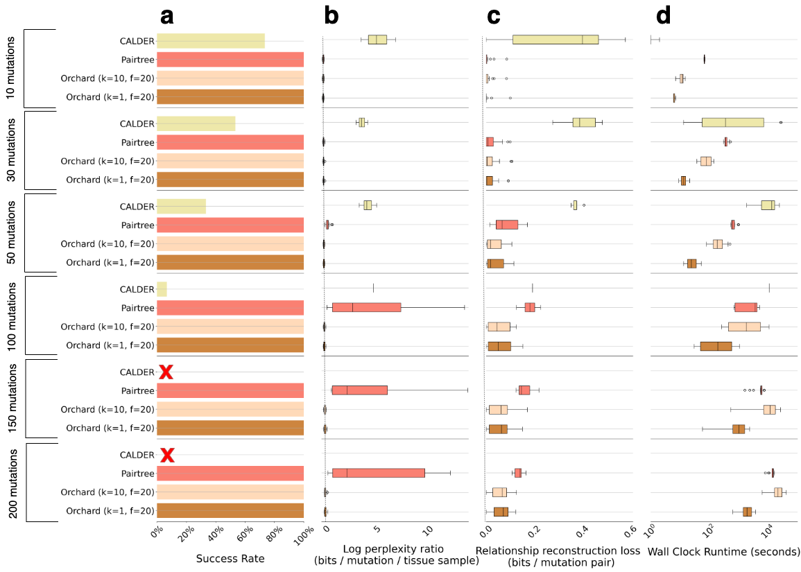
Figure 1: Evaluation of reconstructions for 90 simulated mutation tree data sets. Results are grouped by the size of the simulated mutation trees (rows), i.e., the problem size. a. Bar plots show the percentage of data sets where a method produces at least one valid tree. A red $x$ means the method did not succeed on any of the data sets for that problem size. The distributions, represented by box plots, in (b,c,d) only include data sets where the method was successful. b. The distribution of log perplexity ratios, a measure of VAF data fit. Ratios are relative to the perplexity of the ground truth mutation frequency matrix $F^{(\text{true})}$, and can be negative. c. The distribution of relationship reconstruction loss for each method on a problem size. This loss can range between zero bits (complete match) and one bit (complete mismatch). d. The distribution of wall clock run time.

	Simulated data set size (mutations)
	10		30		50		100		150		200
	P	R	P	R	P	R	P	R	P	R	P	R
CALDER	0	1	0	0	0	0	0	0	0	0	0	0
Pairtree	1	0	4	3	0	0	0	0	0	0	0	0
Orchard (k=1)	8	13	8	9	10	5	4	7	1	8	4	7
Orchard (k=10)	6	1	3	3	5	10	11	8	14	7	11	8

Table 1: Count of simulated mutation tree data sets, out of 15 per column, where a model had the best log perplexity ratio (P) or relationship reconstruction loss (R). Bold indicates column max.

Figure 1 shows the performance of Orchard, CALDER, and Pairtree on the 90 simulated mutation tree reconstruction problems. Table 1 contains counts of data sets, separated by problem size, where a method had the best log perplexity ratio (P) or relationship reconstruction loss (R). CALDER was the only method to fail on a reconstruction problem, its failure rate increased as the problem size increased, and it failed to produce a valid tree on any reconstruction problem with more than 100 mutations.

Figure 1 and Table 1 illustrate a problem-size-dependency in relative performance. Orchard generally outperformed Pairtree and CALDER on the small reconstruction problems (10-30 mutations) on all metrics. Although Orchard’s reconstructions are only slightly better than Pairtree for these problems, Orchard produced these reconstructions 5-10x faster than Pairtree. In contrast, Orchard consistently outperformed Pairtree and CALDER on all problems with 50 or more mutations. For these problems, in either setting of $k$, Orchard is finding trees that are drastically better than those found by Pairtree or CALDER. Orchard ($k=1$) generally outperforms Orchard ($k=10$) on smaller problems (10-30 mutations), but this switches on larger problems. To understand this change, we inspected the trees recovered by Orchard ($k=1$ and $k=10$). In nearly all 10 or 30-mutation tree reconstruction problems, both Orchard configurations found the same best tree. However, Orchard ($k=10$) yields nine other sub-optimal trees which are included in the weighted averages used to compute the metrics resulting in slightly worse average scores. On larger problems, the trees reconstructed by Orchard ($k=10$) are generally much better than those reconstructed by Orchard ($k=1$).

2.3.2 Orchard infers more plausible reconstructions on real data than competing methods

We applied Orchard, CALDER and Pairtree on real bulk DNA data from 14 B-progenitor acute lymphoblastic leukemias (B-ALLs) originally studied in [39]. These B-ALL data sets vary in the number of subclones (between 5 and 17), represented by expert-defined mutation clusters, tissue samples (between 13 and 90), and mutations (between 16 and 292). All of the B-ALL data sets had an approximate sequencing depth of 212x [39]. Each B-ALL patient had samples taken at diagnosis and relapse, and then each of these samples was transplanted into immunodeficient mice resulting in multiple patient derived xenografts (PDXs). The VAF data for each B-ALL data set was used by experts to manually cluster mutations and construct clone trees, both of which were reviewed for biological plausibility [39]. A maximum a posteriori (MAP) mutation frequency matrix $F^{(\text{MAP})}$ was fit to each of the 14 expert-derived clone trees (see A.4.2). Each mutation in $F^{(\text{MAP})}$ is assigned a frequency according to the MAP mutation frequency of the supervariant or subclone the mutation belongs to in the clone tree. These MAP mutation frequency matrices were used to compute a baseline perplexity.

Figure 2a shows the log perplexity ratio for Orchard, CALDER, and Pairtree on the 14 B-ALL data sets. Orchard ($k=1$) had a slightly lower log perplexity ratio than Pairtree on 10 out of 14 B-ALL data sets (average of -2.17e-5 fewer bits). Both Pairtree and Orchard beat the baseline perplexity on one data set (SJBALL031), where Pairtree had a negative log perplexity ratio of -3.86e-4 bits, and both of Orchard’s model setups had a negative log perplexity ratio of -3.57e-4 bits. On the other 13 B-ALL data sets Orchard nearly matched the baseline with an average log perplexity ratio of +1.17e-2 bits and +1.19e-2 bits for $k=1$ and $k=10$, respectively. CALDER failed on 2 of the 14 B-ALL data sets, and performed worse than both Orchard and Pairtree on the data sets where it succeeded. The log perplexity for Orchard, Pairtree and CALDER on each individual B-ALL data set is shown in Supplemental Figure 15.

2.3.3 Orchard infers more plausible mutation trees than Pairtree for 14 leukemias

We then considered an alternative scenario where the expert-derived mutation clusters are not provided for the 14 B-ALL data sets. We compared two approaches to infer clusters and clone trees for this data: $(1)$ the classic approach of using mutation clustering tools to group mutations into subclones and then reconstructing a clone tree on these subclones, or $(2)$ constructing a mutation tree directly on the VAF data for each B-ALL data set, and then clustering connected groups of mutations in the mutation tree. In this section we evaluate mutation trees constructed for $(2)$. In Section 2.3.4, we infer and then evaluate mutation clusters using approaches $(1)$ and $(2)$. In A.10.3, we evaluate the clone trees constructed on the mutation clusters from Section 2.3.4.

The 14 B-ALL cancer data sets contain between 16-292 mutations (median of 40), resulting in very large mutation trees. Since CALDER has a high failure rate on data sets with more than 30 nodes (see Figure 1), we chose to exclude it from this analysis. Since we do not have expert-derived mutation trees for the 14 B-ALL data sets, we use the MAP mutation frequency matrix $F^{(\text{MAP})}$ for each data set’s expert-derived clone tree as a baseline. Figure 2b-c plots the log perplexity ratio for Orchard ($k=10$) and Pairtree on each B-ALL data set, and shows that Orchard matches the performance of Pairtree on reconstruction problems with fewer than 50 nodes, but finds much better trees than Pairtree on those with more than 50 nodes. Notably, on mutation tree reconstruction problems with 129 nodes (SJETV010, Figure 2b) and 292 nodes (SJBALL022610, Figure 2c), Orchard beats Pairtree by more than $3$ and $25$ bits, respectively. The results in Figure 2b-c also show that the mutation trees reconstructed by Orchard always agree with the VAF data better than the expert-derived clone trees. For three particular patients (SJVET047, SJETV010, SJBALL0222610), the mutation trees reconstructed by Orchard have a relative decrease in perplexity that is greater than 1 bit, suggesting the possibility that the expert-derived mutation clusters for these patients are incorrectly grouping distinct subclones together.

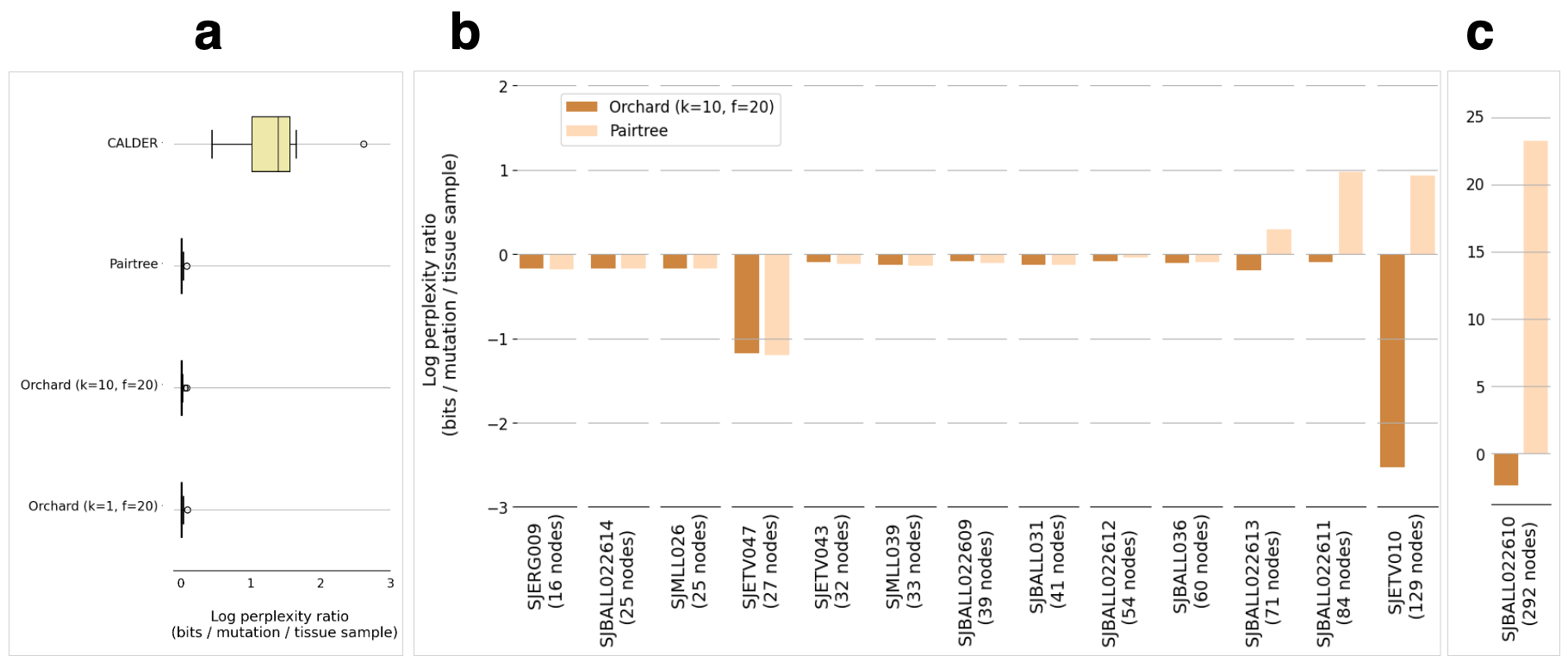
Figure 2: Evaluation of reconstructions on the 14 B-ALL data sets. a. Box plots show the distribution of log perplexity ratio for each method when reconstructing clone trees for the 14 B-ALL data sets. The expert-derived mutation clusters for each data set were provided as pre-defined mutation clusters to all methods. Log perplexity ratio is reported relative to the maximum a posteriori (MAP) mutation frequencies $F^{(\text{MAP})}$ for the expert derived trees. CALDER failed on two data sets, so its box plots only contain data from the other 12. b-c. Bar plots show the log perplexity ratio for the mutation trees reconstructed by Orchard ($k=10$) and Pairtree using the unclustered mutation data for each B-ALL data set. Part c has a larger y-axis range to accommodate Pairtree’s large log perplexity on the 292 node data set. Log perplexity ratio is reported relative to the MAP mutation frequencies $F^{(\text{MAP})}$ for each data set’s expert-derived clone tree.

2.3.4 Phylogeny-aware clustering can infer better mutation clusters than VAF-based clustering

Orchard contains a ’phylogeny-aware’ clustering algorithm that uses a reconstructed mutation tree and its corresponding inferred mutation frequency matrix $F$ to cluster mutations and find clone trees. This algorithm performs agglomerative clustering and joins adjacent nodes $u$ and $v$ using the following formula: $\text{min}_{i\in u,j\in v}{d(u,v)}$, where $d(u,v)=\sqrt{\sum_{s=1}^{m}{(F_{is}-F_{js})^{2}}}$ (see A.7 for more detail). The agglomerative clustering is repeated, successively joining adjacent nodes, until it reaches a clone tree consisting of only the root node and a single node containing all mutations. Each clone tree of size $2,\dots,n+1$ is scored under a binomial likelihood model, and the clone tree that maximizes the Generalized Information Criterion (GIC) [40] is yielded.

Figure 3: Evaluation of ’phylogeny-aware’ clustering versus state-of-the-art VAF-based mutation clustering methods on 14 B-ALL data sets. Adjusted Rand Index, and normalized lineage count similarity are measured in reference to the expert-derived mutation clusters for the 14 B-ALL data sets. Outliers are labeled by their unique ID. a. Box plots show the distribution of the Adjusted Rand Index for each method. b. Box plots show the distribution of the normalized lineage count similarity for each method.

We evaluate our phylogeny-aware clustering algorithm using the expert-derived mutation clusters from the 14 B-ALL data sets. We provided the phylogeny-aware clustering algorithm with the best mutation tree reconstructed by Orchard and Pairtree for each B-ALL data set, corresponding to those in Section 2.3.3. We compare our phylogeny-aware clustering algorithm with three state-of-the-art mutation clustering algorithms that use the VAF data to infer mutation clusters: PyClone-VI [27], VIBER [26], and SciClone [28]. We used two metrics to evaluate the clusters inferred by each method: $(1)$ Adjusted Rand Index (ARI), the percentage of correctly co-clustered mutations adjusted for randomness [41], and $(2)$ Normalized lineage count similarity (LCS), how well a method predicts the number of expert-derived clusters. LCS is a value between 0 and 1, where 1 means the method predicted the same number of mutation clusters as the expert-derived clustering, and 0 means a method greatly overestimated or underestimated the number of mutation clusters.

	ARI	LCS
Pairtree+Cluster	8	8
Orchard+Cluster	9	9
VIBER	2	2
SciClone	1	0
PyClone-VI	6	6

Table 2: Count of B-ALL data sets where a mutation clustering method had the best Adjusted Rand Index (ARI) or the best Normalized Lineage Count Similarity (LCS). Bold indiciates column max. There are a total of 14 B-ALL data sets, however, the counts add up to more than 14 due to ties for the best score.

Figure 3 compares the distributions of clustering metrics for each method. We use ’Orchard+Cluster’ and ’Pairtree+Cluster’ to refer to the phylogeny-aware clustering method applied to mutation trees constructed by Orchard and Pairtree, respectively. Mutation clusters inferred by ’Orchard+Cluster’ were, on average, most similar to the expert-derived mutation clusters. The breakdown of each method’s performance on the individual data sets are shown in Figure 13 (ARI), and Figure 14 (LCS). Table 2 shows the counts of how many data sets a method obtained (or tied) the best score for a metric. Each method only had the best score for both metrics on a subset of data sets: ’Orchard+Cluster’ (SJBALL022613), ’Pairtree+Cluster’ (SJBALL022609), PyClone-VI (SJMLL039, SJETV047), VIBER (None), SciClone (SJETV010, ARI only). Although the phylogeny-aware clustering method matched or outperformed competing mutation clustering methods on the majority of B-ALL data sets, it failed to recover mutation clusters that match the expert-clustering for the largest B-ALL data set containing 292 nodes (SJBALL022610) (see Figure 13).

3 Discussion

Modern cancer evolution studies produce large bulk DNA data sets often containing hundreds of mutations and multiple cancer samples. This vast amount of bulk DNA data presents a promising opportunity to improve our understanding of the evolutionary events that drive cancer progression. Until now, existing mixed sample perfect phylogeny reconstruction algorithms were unable to reliably reconstruct trees with more than 30 mutations. These limitations necessitated clustering mutations prior to reconstructing trees, which is an error prone process [29, 30, 31]. We introduced Orchard, a mixed sample perfect phylogeny reconstruction algorithm that uses variant allele frequency data from bulk DNA sequencing to build large mutation trees. We showed that Orchard can reliably match or beat ground-truth (or expert-derived) baselines on tree reconstruction problems with up to 300 nodes and up to 100 samples from the same cancer. Orchard can recover larger trees on simulated data, and in 12 we use Orchard to successfully reconstruct 1000-node simulated mutation trees in $\approx 27$ hours of wall clock time. Orchard’s ability to reconstruct extremely large trees motivated a new strategy where the mutation tree structure is used to guide the inference of mutation clusters and clone trees. To this end, we introduced a ’phylogeny-aware’ clustering algorithm that uses agglomerative clustering to infer both mutation clusters and clone trees from large mutation trees. Another key contribution of this paper is using the Gumbel-Max trick to turn a combinatorial algorithm that maximize an objective into a stochastic algorithm that samples from it.

There are a few potential areas of improvement for Orchard. First, the majority of Orchard’s run time is used by the projection algorithm [35] to estimate the clonal proportion matrix $U$ each time it extends a tree. Although the computational complexity for estimating $U$ is, at worst, quadratic in the number of mutations (i.e., rows) in $U$, the wall clock times grows quickly with increasing problem size, beam width ($k$), or branching factor ($f$). One potential improvement, because the frequency of most mutations should not be changed by introducing a new node into the tree, is developing a new version of the projection algorithm that only performs local updates to the $U$ matrix. Also, the current implementation of Orchard’s node placement routine has an exponential worst case for the number of node placements when the tree is a star tree where all nodes are children of the root. Unless specified otherwise, Orchard will try all $2^{l}+l$ possible node placements for a star tree consisting of $l$ nodes and the root $r$. Fortunately, under the ISA, such trees are rare and linear branching becomes more likely as the number of children for some node increases. So, in practice, it is likely very rare for nodes to have large numbers of children.

The current version of ’phylogeny-aware’ clustering algorithm uses a simple, non-probabilistic merging strategy to identify mutation clusters on a mutation tree. Despite this, the algorithm already matches, or in some cases, outperforms state-of-the-art probabilistic VAF-based mutation clustering algorithms on both real (Section 2.3.4) and simulated data (12). These results suggest that the mutation tree structure is useful for guiding the inference of mutation clusters and clones trees. We anticipate that improvements to the current algorithm to make it probabilistic, so that its merging choices are made based on an appropriate likelihood function, will result in even greater performance.

We further anticipate the development of new algorithms that take advantage of the large mutations trees reconstructed by Orchard. For example, these trees could be used to study patterns of somatic mutations, recover lineage-specific mutation signature activities, or identify patterns of metastatic spread [16]. Although we did not consider non-cancerous uses of Orchard, one can imagine similar noisy mixed sample perfect phylogeny problems arising in microbiome studies, i.e., when attempting to reconstruct the phylogenies of (non-recombining) microbes based on wastewater samples [42]. The Orchard algorithm could also be adapted to reconstruct mutation trees from single-cell data where there is a large proportion of doublets, though such an adaptation would require updating Orchard’s noise model and sampling routine to accommodate single cell data.

Appendix A Method Detail

A.1 Key Resources Table

RESOURCE	SOURCE	IDENTIFIER
Deposited Data
Simulated mutation tree data shown in Figure 1	This paper	Link
576 simulated clone tree datasets shown in Figure 5	Wintersinger et al., 2022 [24]	Link
B-progenitor acute lymphoblastic leukemias (B-ALLs) data shown in Figure 2a	Dobson et al., 2020 [39]	Link
Chronic Lymphocytic Leukemia (CLL) data shown in Figure 6	Schuh et al., 2012 [14]	Link
Software and Algorithms
Orchard	This paper	Link
Phylogeny-aware clustering	This paper	Link
Pairtree	Wintersinger et al., 2022 [24]	Link
CALDER	Myers et al., 2019 [25]	Link
PyClone-VI	Gillis et al., 2020 [27]	Link
SciClone	Miller et al., 2014 [28]	Link
VIBER	Caravagna et al., 2020 [26]	Link

A.2 Overview

The information in this appendix will be presented in the following order: $(1)$ Data preparation, further details on how Orchard’s inputs are calculated, $(2)$ Evaluation metrics, a thorough detailing of the evaluation metrics used to benchmark Orchard, $(3)$ Orchard algorithm, further details and mathematical derivations for the Orchard algorithm, $(4)$ Phylogeny-aware clustering, further details and mathematical derivations for the phylogeny-aware clustering algorithm, $(5)$ Extended results, results that could not be included in the main paper for the sake of brevity.

A.3 Data preparation

We describe in this section how certain inputs to Orchard can be calculated both in theory and practice. The actual input file formats for Orchard are the same as Pairtree [24], and these inputs have been described in detail in previous protocols [43].

A.3.1 Computing the variant read probability $\omega$

The variant read probability for some mutation $j$ in a bulk cancer sample $s$, which we denote as $\omega_{js}\in[0,1]$, is an estimate of how likely we are to obtain a variant read for the mutant allele $j$ in the sample $s$ when mapping a read to the genomic locus that contains the mutant allele $j$. In order to compute $\omega_{js}$, we require some basic information about the bulk sample $s$. Since all bulk cancer samples consist of some mixture of healthy cells and cancerous cells, it’s important that we have an estimate of the fraction of cancerous cells in the bulk cancer sample, which is commonly referred to as the sample’s purity. We denote the purity of the bulk cancer sample $s$ as $\rho_{s}$, where $\rho_{s}\in[0,1]$. If all of the cells in sample $s$ are cancerous then $\rho_{s}=1$, and if all of the cells in sample $s$ are healthy then $\rho_{s}=0$. We also require allele specific copy number information for the genomic locus containing mutation $j$. Specifically, we need to know the population average copy number of the mutant allele $j$ in sample $s$ which we denote as $M_{js}$, and the population average copy number of the locus containing the mutant allele $j$ which we denote as $N_{js}$.

If sample $s$ contains only cancerous cells, i.e., $p_{s}=1$, then $M_{js}$ and $N_{js}$ are precise population average copy number estimates for the cancerous cell population. If sample $s$ is a mixture of healthy and cancerous cells, i.e., $\rho_{s}<1$, then $M_{js}$ and $N_{js}$ are instead mixtures of the average copy numbers for the healthy cell population and the cancerous cell population proportional to the purity of sample $s$. In general, we can write $M_{js}$ and $N_{js}$ as follows

$$M_{js} =pM^{(c)}_{js}+(1-p)M^{(h)}_{js}$$

$$N_{js} =pN^{(c)}_{js}+(1-p)N^{(h)}_{js}$$

where $M^{(c)}_{js}$ is the population average copy number of the mutant allele $j$ in the cancerous cell population, $N^{(c)}_{js}$ is the population average copy number of the locus containing the mutant allele $j$ in the cancerous cell population, $M^{(h)}_{js}$ is the population average copy number of the mutant allele $j$ in the healthy cell population, and $N^{(h)}_{js}$ is the population average copy number of the locus containing the mutant allele $j$ in the healthy cell population. We always assume that $M^{(h)}_{js}=0$, i.e., that the mutation is not present in the healthy cell population. We can use the definitions of $M_{js}$ and $N_{js}$ to obtain a total population estimate (cancerous cell population + healthy cell population) of the variant read probability for mutation $j$ in the bulk cancer sample $s$ as

$$\omega_{js}=\frac{M_{js}}{N_{js}}$$ (1)

A.3.2 Computing a ’supervariant’ approximation

If Orchard is used to construct a clone tree, then it expects as an input a set of mutation clusters that represent individual clones. In this case, Orchard treats all mutations in the same clone as a single mutation or alternatively a ’supervariant’. A ’supervariant’ is a concept originally from [24] that approximates the data for a set of mutations $C=\{X_{1},X_{2},\dots,X_{j},\dots\}$ as a single mutation. We provide a brief explanation of this approximation scheme but refer the reader to [24] for complete details.

A ’supervariant’ approximation represents a group of mutations as a single mutation, i.e., a single node that can be placed into a mutation tree. If $C$ is a finite set of mutations, then the ’supervariant’ approximation of $C$ combines the data of each mutation $j\in C$ in each samples $s=1,\dots,m$, such that the data for $C$ in sample $s$ can be represented as $X_{Cs}=\left(a_{Cs},b_{Cs},\omega_{Cs}\right)$, where $a_{Cs}$, $b_{Cs}$, and $\omega_{Cs}$ are the reference read count, variant read count, and variant read probability for $C$ in sample $s$, respectively. One issue when combining the mutation data in $C$ is that it is not guaranteed that all mutations $j\in C$ have the same variant read probability in sample $s$, $\omega_{js}$. To resolve this, $\omega_{Cs}=\frac{1}{2}$ is fixed for all samples $s=1,\dots,m$, and the data for all mutations $j\in C$, i.e., $X_{js}=\left(a_{js},b_{js},\omega_{js}\right)$, is scaled as follows:

$$T_{js} =a_{js}+b_{js}$$

$$\widehat{T}_{js} =2\omega_{js}T_{js}$$

$$\widehat{b}_{js} =min(b_{js},\widehat{T}_{js})$$

$$\widehat{a}_{js} =\widehat{T}_{js}-\widehat{b}_{js}$$

$$\widehat{\omega}_{js} =\frac{1}{2}$$

After scaling the data for each mutation $j\in C$ for all samples $s=1,\dots,m$, we can compute the values for $X_{Cs}$ as follows:

$$X_{Cs} =\left\{a_{Cs},b_{Cs},\omega_{Cs}\right\}$$

$$a_{Cs} =round\left(\sum_{j}{\widehat{a}_{js}}\right)$$

$$b_{Cs} =round\left(\sum_{j}{\widehat{b}_{js}}\right)$$

$$\omega_{Cs} =\frac{1}{2}$$

There are a few problems with the ’supervariant’ approximation. First, using the ’supervariant’ approximation results in a slightly different reconstruction problem than a mutation tree reconstruction problem, where the perfect phylogeny matrix $B$ and the clonal proportion matrix $U$ are inferred for the ’supervariants’ instead of the mutations. Also, grouping mutations with different variant read probabilities means that we assume mutations co-occur even though they are in genomic regions that vary in copy number. There is, in fact, uncertainty about whether or not these mutations are part of the same clone if they fall in genomic regions that differ in copy number. Since Orchard can reconstruct extremely large trees, we could instead use a relaxed ’supervariant’ approximation, where pre-defined mutation clusters are split apart such that only mutations with the same variant read probability appear in the same clone. This relaxation would remove some of the pitfalls introduced by the ’supervariant’ approximation. For convenience, we chose to use the ’supervariant’ approximation as described here.

A.4 Evaluation metrics

A.4.1 Perplexity

We use the perplexity to evaluate a cancer phylogeny reconstruction based on the inferred mutation frequency matrix $F$. Assuming we’ve sampled $Q$ total unique trees $S=\{t_{1},t_{2},\dots,t_{q},\dots,t_{Q}\}$ with some probability distribution over this set of trees $0\leq p(t_{q})\leq 1$ with $\sum_{q}{p(t_{q})}=1$, we can compute the perplexity of this set of trees, $PP(S)$, as

$$PP(S) =2^{\epsilon}$$ (2)

$$\epsilon =-\frac{1}{nm}\sum_{j=1}^{n}\sum_{s=1}^{m}log_{2}\left(\sum_{q=1}^{Q}{p\left(X_{js}|F_{js}^{(q)}\right)p(t_{q})}\right)$$ (3)

where $p\left(X_{js}|F_{js}^{(q)}\right)=\text{Binom}(b_{js}|b_{js}+a_{js},\omega_{js}F_{js})$. Equation 3 is the exponent for the likelihood weighted average perplexity of the mutation frequency matrices $\{F^{(q)}:q=1,\dots,Q\}$ under a binomial likelihood model.

We can measure the perplexity of a mutation frequency matrix $F$ reconstructed by a method in reference to a baseline perplexity using the ratio $\frac{2^{\epsilon_{\Omega}}}{2^{\epsilon_{base}}}$, where $\epsilon_{\Omega}$ is equivalent to Equation 3 and $\epsilon_{base}$ is the exponent for the baseline perplexity being compared against. The perplexity at times can be a very large value, and as a result we choose to transform the perplexity and the perplexity ratio using a base 2 logarithmic transformation, i.e., the log perplexity and log perplexity ratio. The log perplexity ratio has also been called the VAF Reconstruction loss in previous work [24]. We denote the log perplexity ratio as $\hat{\epsilon}$, where $\hat{\epsilon}=log_{2}\left(\frac{2^{\epsilon_{\Omega}}}{2^{\epsilon_{base}}}\right)=\epsilon_{\Omega}-\epsilon_{base}$. Therefore, it is possible that $\hat{\epsilon}$ is negative showing that the mutation frequency matrix $F$ for the tree(s) reconstructed by a method fit the VAF data better than the baseline mutation frequency matrix. With simulated data, the baseline is the ground-truth mutation frequency matrix $F^{\text{(true)}}$ used to generate the simulated VAF data. With real data, the baseline is the maximum a posteriori (MAP) mutation frequency matrix $F^{(\text{MAP})}$ fit to the expert derived tree. The MAP mutation frequency matrices fit to the expert-derived trees were calculated using a gradient based method called resilient backpropagation (rprop) [24] (see Supplement Section A.4.2).

A.4.2 Computing the maximum a posteriori mutation frequency matrix for expert-derived trees

In many cases, a bulk DNA clone tree derived by experts does not have an explicit mutation frequency matrix $F$ that adheres to a perfect phylogeny. Instead, we can approximate the mutation frequency matrix by fitting a maximum a posteriori (MAP) estimate of $F$ after observing the expert-derived clone tree. Although Orchard uses the projection algorithm [35] to fit the mutation frequency matrix $F$, this algorithm optimizes an approximation to the likelihood, so it is not guaranteed to find the maximum likelihood estimate. We can instead optimize the unimodal likelihood directly to define $F$ using a gradient based method. Unfortunately, gradient based methods take a long time to converge making them impractical for large reconstruction problems. Gradient based methods are, however, quite useful for fitting a MAP estimate of $F$ on real bulk DNA clone trees derived by experts. One such gradient based method that has been used for this task in prior research is rprop or resilient backpropagation [24]. We chose to use rprop to find the MAP mutation frequency matrix $F^{(\text{MAP})}$ for the expert-derived clone trees for the B-ALL data sets (see Section 2.3.2) and the CLL data sets (see 6). For each real bulk DNA data set, we ran rprop for 30,000 epochs.

A.4.3 Relationship reconstruction loss

The relationship reconstruction loss measures how well the pairwise relationships between mutations in some proposed tree $t_{q}$ match the pairwise relationships in a set of $N$ ground truth trees:

$$S=\left\{t^{(\text{true})}_{1},t^{(\text{true})}_{2},\dots,t^{(\text{true})}_{N}\right\}.$$

We primarily use the relationship reconstruction loss when evaluating reconstructions for simulated mutation tree reconstruction problems. We generated simulated trees and VAF data using the Pearsim software (https://github.com/morrislab/pearsim). The Pearsim software starts with a ground truth mutation frequency matrix $F^{(\text{true})}$, then all possible trees are enumerated that fit $F^{(\text{true})}$ without violating the ISA, resulting in a set of $N$ ground truth simulated trees which we denote as $S$. Since each pair of nodes $(u,v)$ in a tree $t_{q}$ can have one of the three mutually exclusive pairwise relationships (see Definition 1), we define the probability for some pairwise evolutionary relationship in a proposed tree $t_{q}$ as

$$p(R_{uv}=e|t_{q})=\begin{cases}1&\text{ iff }R_{uv}=e\text{ in tree }t_{q}\\ 0&\text{ otherwise},\end{cases}$$

where $e\in\{\text{ancestral},\text{descendant},\text{branched}\}$ as defined in Definition 1, and $R_{uv}$ is the pairwise evolutionary relationship between nodes $u$ and $v$ defined by the tree $t_{q}$.

We can then compute the probability $p(R_{uv}=e)$ for some relationship $e$ given the $Q$ total unique trees sampled by some mutation tree reconstruction method as $p(R_{uv}=e)=\sum_{q=1}^{Q}{p(R_{uv}=e|t_{q}})p(t_{q})$. We can perform the same computation for the set of $N$ true trees, only we use a uniform prior $p(t^{(\text{true})})=\frac{1}{N}$. We denote the posterior distribution over the pairwise relationships in our set of $Q$ proposed trees as $p(R_{uv})$, while we denote the posterior distribution over the pairwise relationships in our set of $N$ true tree as $p(\tilde{R}_{uv})$. We can then measure the difference between these two distributions using the Jensen-Shannon divergence (JSD) while normalizing over the total number of pairs of mutations in the tree

$$\epsilon_{R}=\frac{2}{n(n+1)}\sum_{u,v}{JSD(R_{uv}||\tilde{R}_{uv})}$$ (4)

A.4.4 Pairwise evolutionary relationships

Given a mutation tree $t=\{V,E,M\}$ and an ordered pair of nodes $(u,v)\in V$, there are 3 possible pairwise evolutionary relationships the ordered pair $(u,v)$ can have:

Definition 1 (Pairwise Evolutionary Relationships).

Ancestral: u is an ancestor of v, i.e., v contains the mutation(s) associated with u, but v contains one or more mutations not present in u.

Descendant: v is an ancestor of u, i.e., the same as above but u and v are switched.

Branched: u and v share some common ancestor, but neither u nor v are ancestral to each other.

We can denote the 3 possible pairwise evolutionary relationships from Definition 1 for the ordered pair of nodes $(u,v)$ as one of the following:

$$R_{uv} =\text{ ancestral }$$

$$R_{uv} =\text{ descendant }$$

$$R_{uv} =\text{ branched }$$

where $R_{uv}$ denotes the evolutionary relationship between the ordered pair $(u,v)$. Note that $R_{uv}$ can be derived from the ancestral matrix $B$ associated with $t$ as follows:

$$R_{uv}=\begin{cases}\text{ ancestral }&\text{if}\ B_{uv}=1,B_{vu}=0\\ \text{ descendant }&\text{if}\ B_{uv}=0,B_{vu}=1\\ \text{ branched }&\text{if}\ B_{uv}=B_{vu}=0\end{cases}$$

and if $B_{uv}=B_{vu}=1$ then $B$ is not consistent with any tree, as this implies a cycle.

A.4.5 Adjusted Rand Index

The Rand Index is used to compare two clusterings based on the pairs of elements that co-occur (or do not co-occur) in the same cluster. The adjusted Rand Index is a normalized version of the Rand Index. The Rand Index is a value between 0 and 1, while the adjusted Rand Index is a value between -1 and 1, where a value below 0 is obtained if the difference between the two clusterings is worse than what would be expected if the clusterings were randomly generated. For a bulk DNA data set containing $n$ mutations, there are $\binom{n}{2}$ possible pairs of mutations. A mutation clustering algorithm groups together subsets of these $n$ mutations into a finite number of clusters. Let $P$ be the set of all pairs of mutations defined by the clusters constructed by a mutation clustering algorithm. Similarly, let $T$ be the set of all pairs of mutations defined by the baseline (i.e., ground truth or expert-derived) mutation clusters. The number of correct pairs (i.e., true positives) of mutations identified by a mutation clustering algorithm can be computed at $TP=|P\cap T|$, where $TP$ denotes the number of true positives. Similarly, the number of incorrect pairs (i.e., false positives) can be computed as $FP=|P\setminus T|$, where $FP$ denotes the number of false positives. The number of pairs of mutations in $T$ that were not recovered by the mutation clustering algorithm (i.e., false negatives) can be computed as $FN=|T\setminus P|$, where $FN$ denotes the number of false negatives. Finally, the number of pairs of mutations that do not appear in either the proposed clusters output by a mutation clustering algorithm or the baseline clusters (i.e., true negatives) can be computed as $TN=|(A\setminus P)\cap(A\setminus T)|$, where $A$ is the set of all $\binom{n}{2}$ possible pairs of mutations, and $TN$ denotes the number of true negatives. The Rand Index can be defined in terms of the number of pairs of mutations that are classified as true positives (TP), false positives (FP), false negatives (FN), and true negatives (TN). We can compute the Rand Index as

$$RI=\frac{TP+TN}{TP+FP+FN+TN},$$ (5)

and we can compute the adjusted Rand Index as

$$ARI=\frac{2(TP\times TN-FN\times FP)}{((TP+FN)\times(FN+TN)+(TP+FP)\times(FP+TN))}$$ (6)

A.4.6 Normalized lineage count similarity

The normalized lineage count similarity is a metric originally from [29]. The normalized lineage count similarity attempts to measure how well a mutation clustering algorithm estimates the number of clones (i.e., mutation clusters) there are in an individual cancer. If the baseline (i.e., ground truth or expert-derived) clustering has $L$ clusters, and a mutation clustering algorithm estimates that there are $\kappa$ clusters, then the normalized lineage count can be calculated as

$$\frac{L-min(|\kappa-L|,L+1)+1}{L+1}$$ (7)

The normalized lineage count simiarlity is a metric between $0$ and $1$, where $0$ means that the mutation clustering algorithm greatly overestimates or underestimates the number of clusters, while $1$ means that the mutation clustering algorithm predicts that there are exactly $L$ clusters.

A.5 Orchard algorithm

In this section, we provide further details about the Orchard algorithm. Algorithm 1 provides the pseudocode for the Orchard algorithm. In A.5.1, we provide a more comprehensive explanation for how we propose the order in which Orchard will add nodes to the tree. In A.6, we provide the mathematical derivations for how we can evaluate the different placements of some node $u$ into a partial tree $t^{(l)}$.

input: A dataset $D$ containing allele frequency data and copy number information for $n$ mutations in $m$ tissue samples

parameters: k (beam width), f (branching factor)

output : $k$ unique complete trees with the best total perturbed log-probabilities

1

$Q\leftarrow PriorityQueue()$ ;

  // Initialize Q as a priority queue

$Q.size\leftarrow k$ ;

  // make it so Q holds at most $k$ partial trees

$Q.push(Tree())$;

  // insert a partial tree consisting of only the root node into Q

2 while $Q.size\neq 0$ do

       // pop partial tree $t^{(l)}$ from Q, where $l$ is the partial tree size s.t. $0\leq l\leq n$

       $t^{(l)}\leftarrow Q.pop()$ // get one of the $n-l$ remaining mutations not yet in $t^{(l)}$

       $u\leftarrow getNextMutation(t^{(l)})$ // sample $f$ unique placements of mutation $u$ in $t^{(l)}$ and score them

       // $possibleTrees$ is an array of $f$ unique partial trees of size $l+1$

       $possibleTrees\leftarrow sampleTrees(D,t^{(l)},u,f)$ // perturb log-probability of each partial tree using Gumbel-max trick (see Section 2.3)

3       $perturbedTrees\leftarrow perturbTreeLogProbs(possibleTrees)$

      // If the trees in $perturbedTrees$ are constructed on all $n$ nodes, then we’ll return the one with the best perturbed log-probability

4       if $l==n$ then

5             $Q.size=Q.size-1$

6             yield max(perturbedTrees)

7      else

8             foreach $t^{(l+1)}\in perturbedTrees$ do

                   // Add all partial trees $t^{(l+1)}$ to Q

                   // If the total perturbed log-probability for $t^{(l+1)}$ is not among the top $k$ in Q, Q will discarded it

9                   $Q.push(t^{(l+1)})$

Algorithm 1 Orchard

A.5.1 Proposing the next node

We now turn our focus towards how to select the next node $u\in V\setminus\{r\}$ to place into the tree $t^{(l)}$. As previously stated, the Orchard algorithm begins with a partial tree $t^{(l)}$ where $l=0$, consisting of only the root node which represents a non-cancerous (germline) population from which all clones are descended from. We then add a single node at a time to $t^{(l)}$ using the process described in A.6. Prior to the execution of Orchard, we can propose an order by which to add nodes to $t$ either by sampling an ordering based on the observed VAF data, or by generating a random node ordering. The node placement procedure described in A.6 permits an arbitrary ordering by which to add nodes to $t^{(l)}$, however, a randomized node ordering may result in nodes being placed into the tree long before their ancestors. As the tree structure is built out around some node $u$, the range of integration used in the node placement likelihood function described in A.6 may become arbitrarily restricted near $u$. This can result in $u$’s ancestors not being placed correctly, and these nodes may end up in other parts of the tree structure. In some circumstances, this could be beneficial as Orchard may find a variety of interesting tree structures that fit the VAF data well. An alternative to randomizing the order is to use the observed VAF data to propose an ordering.

A.5.2 Proposing a node ordering using $\widehat{F}$

We can propose a node ordering using the observed mutation frequency matrix $\widehat{F}$. Let $u,v\in V$ be nodes and $u\neq v$. As previously stated, assuming $\widehat{F}$ is noise free, then under the ISA a node $u$ cannot be a descendant of $v$ if $\sum_{s=1}^{m}{\widehat{F}_{us}}>\sum_{s=1}^{m}{\widehat{F}_{vs}}$. If $\widehat{F}$ contains noise, this inequality will still often hold, especially if $m$ is large. In either the noise free or noisy case, if $\sum_{s}^{m}{\widehat{F}_{us}}>\sum_{s}^{m}{\widehat{F}_{vs}},\forall v\in V,v\neq u$, then the further node $u$ is placed away from the root (i.e., placed further down some branch of the tree), the more likely the placement of node $u$ will violate the ISA (see Definition 2, Property 2). Using this information, we can propose a node ordering based on the sum of each node’s observed mutation frequencies across all samples:

$$argsort_{u}\left(\widehat{F}\right)=\left|\sum_{s=1}^{m}{\widehat{F}_{us}}\geq\sum_{s=1}^{m}{\widehat{F}_{vs}},u\neq v\right|$$ (8)

We denote this node ordering approach the $\widehat{F}$ sum node order. Although more complicated procedures could be devised for proposing a node ordering, this approach is a principled problem specific optimization that is fast to perform. In Figure 9, we provide a comparison of the the random node ordering approach to the $\widehat{F}$ sum approach on the 90 simulated mutation tree data sets. We discuss the results for Figure 9 in A.10.5.

A.6 Placing a node into the tree

Given some partial tree $t^{(l)}=\left\{V^{(l)},E^{(l)},M^{(l)}\right\}$ with $l<n$, for which we’ve fit the mutation frequency matrix $F^{(l)}$, we would like to select a node $u\in\bar{V}=V\setminus V^{(l)}$, and place it into $t^{(l)}$ such that its placement maximizes adherence with the ISA. We can enumerate the possible placements of $u$ in $t^{(l)}$ by placing $u$ into $t^{(l)}$ with respect to some node $v$ that’s already in $t^{(l)}$, i.e., $v\in V^{(l)}$. Let $ch(v)$ be the set of children of $v$ according to the tree structure defined by $t^{(l)}$, and let $\mathcal{P}(ch(v))$ be the set of all subsets of $ch(v)$, where $\mathcal{P}(X)$ denotes the powerset of $X$. All unique placements of $u$ with respect to $v$ can be enumerated by fixing $u$ such that it’s a direct descendant of $v$, and then considering separately $u$ as the direct ancestor of each set $\tau$ where $\tau\in\mathcal{P}(ch(v))$. By performing this process for each $v\in V^{(l)}$ we end up considering all possible placements of $u$ in $t^{(l)}$. We can define the placement of $u$ with respect to $v$ in terms of its modifications to $V^{(l)}$ and $E^{(l)}$ in order to obtain a resulting partial tree of size $l+1$, $t^{(l+1)}=\left\{V^{(l+1)},E^{(l+1)},M^{(l+1)}\right\}$:

$$t^{(l+1)}=\left\{V^{(l)}\cup\{u\},\left(E^{(l)}\setminus\left\{(v,c):c\in\tau\right\}\right)\cup\left\{(v,u)\right\}\cup\left\{(u,c):c\in\tau\right\},\left(M^{(l)},u\right)\right\}.$$ (9)

It’s important to note that it’s always the case that the empty set $\emptyset$ is part of $\mathcal{P}(ch(v))$, i.e., $\emptyset\in\mathcal{P}(ch(v))$. As a result, we always consider the placement where $u$ is a direct descendant of $v$, and $u$ has no descendants.

Under the ISA, the mutation frequency matrix $F$ has three important properties in relation to each node $v\in V^{(l)}$ for all tissue samples $s=1,\dots,m$:

Definition 2 ($F$ Properties).

1. $0\leq F_{vs}\leq 1$

2. $F_{vs}\geq\sum_{w\in ch(v)}{F_{ws}}$

3. $F_{vs}=U_{vs}+\sum_{w\in D(v)}{U_{ws}}$

where $D(v)$ denotes the set of all descendants of $v$ according to the tree structure defined by $t^{(l)}$. The value $U_{vs}$ denotes the clonal proportion of node $v$ in sample $s$ where

$$U_{vs}=F_{vs}-\sum_{w\in ch(v)}{F_{ws}}$$ (10)

Once $u$ is placed in $t^{(l)}$, it must also be the case that $F_{us}$ adheres to the constraints in Definition 2. We can use this fact to compute a probability distribution over the placement of $u$ in $t^{(l)}$ based on how well the VAF data for $u$ in each sample $s=1,\dots,m$, $X_{us}=\left\{a_{us},b_{us},\omega_{us}\right\}$, supports the constrained values of $F_{us}$.

Another important relationship we assume for $F_{us}$ is that

$$F_{us}=\frac{\lambda_{us}}{\omega_{us}}$$ (11)

where $\lambda_{us}$ is the variant allele frequency of node $u$ in sample $s$, and $\omega_{us}$ is the variant read probability of node $u$ in sample $s$.

A.6.1 Defining constraints on $F_{us}$ given the placement of $u$

Let us first consider the case where $u$ is placed into $t^{(l)}$ with respect to $v$ and $\tau\neq\emptyset$. We can use Definition 2, Property 2, to define a set of constraints on $F_{us}$. Since $u$ is now the direct ancestor of the nodes in the set $\tau$, it must be the case that

$$F_{us}\geq\sum_{i\in\tau}{F_{is}}$$

At the same time, since $u$ is now a direct descendant of $v$, it must also be the case that

$$F_{vs}\geq F_{us}+\sum_{j\in ch^{*}(v)}{F_{js}}$$

where $ch^{*}(v)=ch(v)\setminus\tau$ is the set of nodes that remain as direct descendants of $v$. We can combine these two inequalities to obtain the following constraints on $F_{us}$

$$F_{vs}-\sum_{j\in ch^{*}(v)}{F_{js}}\geq F_{us}\geq\sum_{i\in\tau}{F_{is}}$$ (12)

We can then use Equation 11 to rewrite Equation 12 as

$$F_{vs}-\sum_{j\in ch^{*}(v)}{F_{js}} \geq\frac{\lambda_{us}}{\omega_{us}}\geq\sum_{i\in\tau}{F_{is}}$$

$$\omega_{us}\left(F_{vs}-\sum_{j\in ch^{*}(v)}{F_{js}}\right) \geq\lambda_{us}\geq\omega_{us}\left(\sum_{i\in\tau}{F_{is}}\right)$$ (13)

where $\lambda_{us}$ is the variant allele frequency (VAF) of node $u$ in sample $s$ and $\omega_{us}$ is the variant read probability of node $u$ in sample $s$ (see Section 2.1 for more details). It’s clear from Equation A.6.1 that if $\tau\neq\emptyset$, then under the ISA $\lambda_{us}$ needs to fall below $\omega_{us}\left(F_{vs}-\sum_{j\in ch^{*}(v)}{F_{js}}\right)$, and above $\omega_{us}\left(\sum_{i\in\tau}{F_{is}}\right)$.

Let us now consider the case where $\tau=\emptyset$. Since again $u$ is a direct descendant of $v$, we can use Definition 2, Property 2, to derive the constraint:

$$F_{vs}\geq\sum_{i\in ch(v)}{F_{is}}+F_{us}$$

By rearranging terms we obtain the following

$$F_{vs}-\sum_{i\in ch(v)}{F_{is}} \geq F_{us}$$

$$U_{vs} \geq F_{us}$$ (14)

$$U_{vs} \geq\frac{\lambda_{us}}{\omega_{us}}$$

$$\omega_{us}U_{vs} \geq\lambda_{us}$$ (15)

The constraint on the left hand side in Equation 14 is obtained by the definition of the clonal frequency $U_{vs}$ (Equation 10). We again use Equation 11 to obtain our final result in Equation 15.

Finally, we can use the constraints in Equation A.6.1 and Equation 15 to define probabilities for the possible node placements of $u$ with respect to $v$:

$$p\left(u,v,\tau|\tau\neq\emptyset\right) =Pr\left[\omega_{us}\left(F_{vs}-\sum_{j\in ch^{*}(v)}{F_{js}}\right)\geq\lambda_{us}\geq\omega_{us}\left(\sum_{i\in\tau}{F_{is}}\right)\right]$$ (16)

$$p\left(u,v,\tau|\tau=\emptyset\right) =Pr\left[\omega_{us}U_{vs}\geq\lambda_{us}\right]$$ (17)

It’s important to reiterate that in practice Equation 16 is computed for all $\tau\in\mathcal{P}(ch(v))$. Notice that the size of $\mathcal{P}(ch(v))$ grows exponentially in the size of $ch(v)$, i.e., if $v$ has $N$ direct children, then there are $\sum_{i=0}^{N}{\binom{N}{i}}=2^{N}$ total elements in $\mathcal{P}(ch(v))$. It’s possible that the VAF data implies such a tree structure, however, it is very unlikely if the point mutations have non-zero VAFs in one or more samples. This is because as the number of children $v$ with non-zero VAFs increases, the more likely it is that Definition 2 is violated, making a perfect phylogeny star tree increasing less likely. In any case, Orchard has a parameter that can be set by the user which limits the number of node placements that are scored using Equation 16. This parameter is called the max placements parameter, and it provides an upper limit on the number of $v$’s children that $u$ can parent. For example, if the max placements is set to 5, then the node placement function will consider all possible placements where $u$ is a child of $v$, and $u$ is the parent of any combination of $i$ children of $v$, where $i=0,\dots,5$. As a result, the node placement function will consider $\sum_{i=0}^{5}{\binom{N}{i}}$ possible placements of $u$ with respect to $v$.

A.6.2 Computing the posterior over $\lambda_{us}$

Under a binomial VAF likelihood model, we assume that our observed variant allele counts $b$ are binomially distributed according to some success probability $\lambda$, and that we’ve mapped a total of $N=a+b$ reads to that locus. We place no prior beliefs on the distribution of $\lambda$, and therefore use a uniform $Beta$ prior on its distribution. We can now define a posterior distribution for $\lambda$ for some mutation $u$ in sample $s$ as follows:

$$b|\lambda_{us} \sim Binom(N_{us},\lambda_{us})$$

$$\lambda_{us} \sim Beta(\alpha_{0},\beta_{0})$$

$$\lambda_{us}|(b=b_{us}) \sim Beta(\alpha_{0}+b_{us},\beta_{0}+N_{us}-b_{us})$$

where $N_{us}=a_{us}+b_{us}$, and the Beta prior is uniform, so $\alpha_{0}=\beta_{0}=1$. Because the $Beta$ is conjugate to the the binomial, the posterior distribution of $\lambda_{us}$ is also a $Beta$ distribution, in this case with $\alpha=1+b_{us}$ and $\beta=1+a_{us}$. We can rewrite the posterior in terms of solely $\lambda_{us}$ and $X_{us}$, where $X_{us}=\left\{a_{us},b_{us},\omega_{us}\right\}$ as follows:

$$p(\lambda_{us}|X_{us}) \propto p(X_{us}|\lambda_{us})p(\lambda_{us})$$

$$\propto f(\lambda_{us},\alpha,\beta)$$ (18)

where $f(\lambda,\alpha,\beta)$ is the probability density function of the Beta Distribution. If we denote $y_{s}=\omega_{us}\left(\sum_{i\in\tau}{F_{is}}\right)$ and $z_{s}=\omega_{us}\left(F_{vs}-\sum_{j\in ch^{*}(v)}{F_{js}}\right)$, then we can define Equation 16 as follows:

$$p\left(u,v,\tau|\tau\neq\emptyset\right) =Pr\left[z_{s}\geq\lambda_{us}\geq y_{s}\right]$$

$$=\int_{y_{s}}^{z_{s}}{f(\lambda_{us},\alpha,\beta)d\lambda_{us}}$$

$$=\int_{y_{s}}^{z_{s}}{\frac{1}{B(\alpha,\beta)}\lambda_{us}^{\alpha}(1-\lambda_{us})^{\beta}d\lambda_{us}}$$

$$=\frac{1}{B(\alpha,\beta)}\int_{y_{s}}^{z_{s}}{\lambda_{us}^{\alpha}(1-\lambda_{us})^{\beta}d\lambda_{us}}$$

$$=I_{z_{s}}(\alpha,\beta)-I_{y_{s}}(\alpha,\beta)$$ (19)

where $I_{x}(\alpha,\beta)$ is the regularized incomplete beta function. If we let $z^{\prime}_{s}=\omega_{us}U_{vs}$, then we can perform a similar process to define Equation 17 as

$$p\left(u,v,\tau|\tau=\emptyset\right) =Pr\left[z^{\prime}_{s}\geq\lambda_{us}\right]$$

$$=\int_{0}^{z^{\prime}_{s}}{f(\lambda_{us},\alpha,\beta)d\lambda_{us}}$$

$$=\frac{1}{B(\alpha,\beta)}\int_{0}^{z^{\prime}_{s}}{\lambda_{us}^{\alpha}(1-\lambda_{us})^{\beta}d\lambda_{us}}$$

$$=I_{z^{\prime}_{s}}(\alpha,\beta)$$ (20)

It’s possible that $y_{s}$ and $z_{s}$ can be very close in Equation 19. This might occur when mutations are part of the same clone, and therefore have very close mutation frequencies across all samples. In this case, we would like Orchard to place these mutations together in the tree, however, the closeness of the mutation frequencies may make it so the ideal placements have near zero probability. To mitigate this problem, we use the mutation frequencies in $F$ and the VAF to compute confidence intervals (upper confidence limit on $z_{s}$, and lower confidence limit on $y_{s}$) to widen the region in which we integrate over $\lambda_{us}$. This may allow these placements to have non-zero probabilities, and are then more likely to be in the top-$f$ node placements.

A.6.3 Sampling $f$ placements of $u$ in $t^{(l)}$

Given some partial tree $t^{(l)}$ for which we’ve fit the mutation frequency matrix $F^{(l)}$, we can use Equation 19 and Equation 20 to score all possible placements of node $u$ in $t^{(l)}$. Let $S$ be the set of scores for all possible placements of $u$ in $t^{(l)}$, i.e., $S=\{p(u,v,\tau):\forall v,\tau\}$. We will choose a subset $S^{\prime}\subseteq S$ where $S^{\prime}$ contains the $f$ largest probabilities associated with unique placements of $u$ in $t^{(l)}$. The resulting $f$ trees of size $l+1$ in the set $S^{\prime}$ will be scored according to the process described in Section 2.3.

A.6.4 Determining the correct branching factor, $f$

Since Orchard’s node placement method computes a probability for each placement of node $u$ into a tree $t^{(l)}$, we can rank each placement by their probability. Thus, the node placement with the largest probability would be considered to be of rank 1, the node placement with the second largest probability would be considered to be of rank 2, etc.. We can then construct trees with Orchard, and record which node placement ranks led us to the highest scoring tree. This helps us evaluate how well our node placement methodology is working, and it helps us empirically determine how many trees with different placements of node $u$ we might need to score to ensure that our search returns trees that fit the VAF data well.

We empirically determined the value of the branching factor $f$ to use in our experiments using a validation set. We ran Orchard on this validation set with a set of parameters that allows it to fit the mutation frequency matrix $F$ to every possible placement of node $u$ in tree $t^{(l)}$, and each mutation frequency matrix $F$ was scored under a binomial likelihood model. Orchard will score every placement of node $u$ in tree $t^{(l)}$ if the branching factor is not limited, i.e., $f=\infty$. This does not result in a complete exhaustive enumeration of all possible trees (which would be computationally intractable for the tree sizes in the validation set), because we limit the number of partial trees to keep track of by setting the beam width parameter $k$. We chose to run Orchard with two different beam widths $k=1$ and $k=10$, along with $f=\infty$. We decided to use 200 simulated bulk DNA cancer phylogenies originally from [25] as a validation set. These simulated bulk DNA cancer phylogenies were meant to simulate whole exome sequencing, and each dataset has between 100-200 mutations, 5 samples, and a read depth of 200x.

Figure 4 shows the percentage of node placement ranks that led to the tree with the highest log-likelihood across all datasets in the validation set. Setting $k=1$ and $k=10$ results in very similar distributions of node placement ranks, therefore we only show Figure 4 which was obtained using Orchard with $k=1,f=\infty$. The 30th percentile for this curve is of rank 21, the 50th percentile is of rank 46, and the 80th percentile is of rank 109. Generally, to capture about 80% of the best node placements, we would have to fit the mutation frequency matrix $F$ and score the top 100 node placements. This is computationally tractable, however, in practice we found on the validation set that the results were still very good and 5x faster when scoring only fitting the mutation frequency matrix $F$ and scoring the top 20 node placements. As a result of these findings on our validation data, we chose to limit $f=20$ in our experiments.

The results in Figure 4 generally support that our node placement function helps us find the correct node placement without having to fit the mutation frequency matrix $F$ for every possible node placement. That being said, further improvements to the node placement scoring function could dramatically decrease run times and improve reconstructions.

Figure 4: The percentage of node placement ranks that led to the tree with the highest log-likelihood across all data sets in the validation set. This was generated using Orchard $(k=1,f=\infty$) and the validation set consisted of 200 simulated cancers originally from [25]. The red dotted line is a Gaussian distribution fit to the node placement rank data.

A.6.5 Adapting the Ancestral Gumbel Top-k trick

Gumbel-Max tricks have been used in prior phylogenetic tree inference methods [44], but to our knowledge none have used the Ancestral Gumbel-Max trick [32, 33]. We will now show how the Ancestral Gumbel Top-k trick described in [32, 33] can be adapted to sample mutation trees.

First, let’s assume we want to construct a mutation tree consisting of $n$ mutations, and that the mutation tree is rooted at a root node $r$ that represents the germline DNA. We also assume the order in which mutations are added to the tree is fixed. The sample space over all partial mutation trees and complete mutation trees can itself be represented as a tree structure, where each node $y_{i}^{(l)}$ at depth $l$ in the sample space tree represents the $i$th unique mutation tree constructed on exactly $l$ mutations. At each level $l$ in the sample space tree, there are $(l+1)^{l-1}$ nodes which represent the $(l+1)^{l-1}$ unique mutation trees that can be constructed on exactly $l$ mutations and a known root $r$. The leaf nodes of the sample space tree, $y_{i}^{(n)}$, represent all possible complete mutation trees constructed on $n$ nodes. Let $t^{(l)}$ be some mutation tree constructed on $l$ nodes, and let $y_{i}^{(l)}$ be the node that represents $t^{(l)}$ in the sample space tree. In some cases, we use $y_{i}^{(l)}$ and $t^{(l)}$ interchangeably. Each node $y_{i}^{(l)}$ at depth $l>0$ in the sample space tree has exactly one parent node $pa\left(y_{i}^{(l)}\right)$ at depth $l-1$, and $t^{(l)}$ is the same as the mutation tree represented by its parent node $pa\left(y_{i}^{(l)}\right)$, $t^{(l-1)}$, with the addition that the $l$th mutation has been placed into $t^{(l-1)}$. Starting from the root of the sample space tree, we can traverse the entire sample space tree in either a breadth-first or depth-first manner, and enumerate all possible ways that the $(n+1)^{n-1}$ complete mutations trees constructed on $n$ mutations can be built when adding a single mutation at a time. We already know that we can score the mutation tree represented by $y_{i}^{(l)}$ as $p(t^{(l)})=p\left(D|F^{(l)}\right)$, where $D$ is the bulk DNA data and $F^{(l)}$ is the mutation frequency matrix computed for $t^{(l)}$. Let $ch\left(y_{i}^{(l)}\right)=\left\{y_{1}^{(l+1)},y_{2}^{(l+1)},\dots,y_{j}^{(l+1)}\right\}$ be the $j$ children of $y_{i}^{(l)}$ in the sample space tree, and let $t^{(l+1)}\in ch\left(y_{i}^{(l)}\right)$ be a mutation tree represented by any node in $ch\left(y_{i}^{(l)}\right)$, and let $F^{(l+1)}$ be the mutation frequency matrix computed for $t^{(l+1)}$ using the algorithm described in [35]. We know by definition that all of the evolutionary relationships among the mutations in $t^{(l)}$ are maintained in $t^{(l+1)}$, and that $t^{(l+1)}$ has additional evolutionary relationships introduced by adding the $l+1$ mutation. Since $F^{(l)}$ is the closest projection of $\widehat{F}^{(l)}$ that adheres to the perfect phylogeny constraints in $t^{(l)}$, it must be the case that $p\left(D|F^{(l+1)}\right)\leq p\left(D|F^{(l)}\right)$, because introducing the constraints from adding the $l+1$ mutation can only further limit the feasible range that the values of $F^{(l+1)}$ can take on. Using this fact, it must be the case that for some node $y_{i}^{(l)}$ that represents the tree $t^{(l)}$, that $p\left(D|F^{(l)}\right)$ is an upper bound on the likelihood for all completions of the tree $t^{(l)}$.

Let $\pi^{(l)}=\text{log}(p(t^{(l)}))$ and $\pi^{(l+1)}=\text{log}(p(t^{(l+1)}))$ where $t^{(l)}$ and $t^{(l+1)}$ are defined according to the nodes $y_{i}^{(l)}$ and $y_{i}^{(l+1)}$ in the sample space tree. We will now derive the Ancestral Gumbel-Max trick for sampling mutation trees. The following derivation is very similar to that shown in [32]. The Gumbel-Max trick is a technique for sampling from a categorical distribution using unnormalized probabilities [37]. Let $H_{\pi}(\mu)=\text{exp}(-\text{exp}(\pi-\mu))$ be the CDF of the Gumbel distribution, and let $H^{-1}_{\pi}(u)=-\text{log}(-\text{log}(u))$ be the inverse CDF of the Gumbel distribution. We can use $H^{-1}_{\pi}$ to generate random Gumbel noise $g\sim\text{Gumbel}(0,1)$ using inverse transform sampling, $g=H^{-1}_{0}(u)$, where $u\sim Uniform(0,1)$ and $\text{Gumbel}(0,1)$ is the Gumbel distribution with a mean of 0 and a variance of 1. Using the shifting property of the Gumbel distribution, the following are equivalent $\pi^{(l)}+g=\pi^{(l)}-\text{log}(-\text{log}(z))\sim\text{Gumbel}(\pi^{(l)})$. We call $G_{\pi^{(l)}}\sim\text{Gumbel}(\pi^{(l)})$ the perturbed log probability of $t^{(l)}$, where $G_{\pi^{(l)}}=\pi^{(l)}+\text{Gumbel}(0,1)$. We can use these definitions to sample the best extension of $t^{(l)}$ as $\operatorname{argmax}_{t^{(l+1)}}{G_{\pi^{(l+1)}}}\sim\text{Categorical}\left(\frac{\text{exp}(\pi^{(l+1)})}{\sum\text{exp}(\pi_{t^{(l+1)^{\prime}}})}\right)$. We can sample the top-$k$ complete mutation trees according to their perturbed log-probabilities as $t_{1}^{*},\dots,t_{k}^{*}=\operatorname{argtopk}{G_{\pi_{t^{(n+1)}}}}$. This is equivalent to instantiating the entire sample space tree, and then sampling the leaf nodes of the sample space tree that have the top-$k$ perturbed log-probabilities.

For any mutation tree $t^{(l)}$ represented by the node $y_{i}^{(l)}$ in the sample space tree, we know that if $t^{(l+1)}$ is an extension of $t^{(l)}$, then $p\left(D|F^{(l+1)}\right)\leq p\left(D|F^{(l)}\right)$. We must also ensure that $p\left(D|F^{(l+1)}\right)+\text{Gumbel}(0,1)\leq p\left(D|F^{(l)}\right)+\text{Gumbel}(0,1)$, or equivalently, $G_{\pi^{(l+1)}}\leq G_{\pi^{(l)}}$. Similarly to how $p\left(D|F^{(l)}\right)$ provides an upper bound on the probability of all completions of $t^{(l)}$, the value of $G_{\pi^{(l)}}$ provides a stochastic upper bound on the perturbed log-probability of all the possible completions of $t^{(l)}$. Since $G_{\pi^{(l)}}$ is a stochastic upper bound for all extensions of $t^{(l)}$, the value of $G_{\pi_{t^{{(l+1)}}}}$ must be smaller than $G_{\pi_{t^{{(l)}}}}$, and so we must sample $G_{\pi^{(l+1)}}$ conditionally on $G_{\pi^{(l)}}$. Let $T=G_{\pi^{(l)}}$, and $Z=\max_{i}{G_{\pi^{(l+1)}}}$. We can sample each extension $G_{\pi^{(l+1)}}$ conditionally on $G_{\pi^{(l)}}$ by truncating $G_{\pi^{(l+1)}}$ at $T$. We perform conditional sampling using the following transformation $\tilde{G}_{\pi^{(l)}}=H^{-1}_{\pi^{(l)},T}\left(H_{\pi^{(l)},Z}\left(G_{\pi^{(l)}}\right)\right)=-\text{log}(\text{exp}(-T)-\text{exp}(-Z)+\text{exp}(-G_{\pi^{(l)}}))$, where $H^{-1}_{\pi^{(l)},T}(u)=\pi-\text{log}(\text{exp}(\pi-T)-\text{log}(u))$ is the inverse CDF of the truncated Gumbel distribution. The full proof of correctness for this transformation can be found in [32]. For complete mutations trees constructed on $n$ nodes, the perturbed log-probability $G_{\pi^{(n)}}\sim\text{Gumbel}(\pi^{(n)})$ can be sampled independently. This means the top-$k$ complete mutation trees can be found by starting from the root of the sample space tree, and searching only parts of the tree that contain the top-$k$ leaf nodes with the largest total perturbed log-probabilities.

A.7 Phylogeny-aware clustering

The ’phylogeny-aware’ clustering algorithm we propose consists of two steps: $(1)$ agglomerative clustering, and $(2)$ model selection. We will now describe these steps in detail.

A.8 Agglomerative clustering

The phylogeny-aware clustering algorithm we propose is an agglomerative clustering algorithm. Agglomerative clustering, also known as hierarchical agglomerative clustering, is a greedy clustering method that iteratively merges pairs of nodes in a graph until the graph consists of only a single node [45]. Generally, agglomerative clustering methods have a worst case time complexity of $O(n^{3})$ [45]. In order to determine which pair of nodes should be combined at each step during agglomerative clustering, a cluster linkage criterion is used to evaluate the dissimilarity between all adjacent nodes in the graph. Since adjacent nodes $u$ and $v$ contain one or more objects (mutations), the cluster linkage criterion is generally a function of the dissimilarity between each pair of objects (mutations) $(i,j)$ where $i\in u,j\in v$.

We use the single linkage criterion, i.e., $\text{min}_{i\in u,j\in v}{d(u,v)}$, and use the Euclidean distance for $d(u,v)$, i.e., $d(u,v)=\sqrt{\sum_{s=1}^{m}{(F_{is}-F_{js})^{2}}}$. There are many different possible cluster linkage criterions and distance metrics, however, we chose the single linkage criterion and Euclidean distance based on results from trying a variety of combinations of distance metrics and linkage criterions on a validation set.

A.9 Model selection for phylogeny-aware clustering

The phylogeny-aware clustering method outputs $n$ different models as a result of its agglomerative clustering scheme. Each model contains a unique number of clusters from $1$ to $n$. We can then either manually select the number of clusters believed to be in the data set (see Figure 7), or we can use a model selection criterion to choose the number of clusters. One of the most well known model selection criterion’s is the Bayesian Information Criterion (BIC) [46]. The BIC chooses a model from a finite set of proposed models based on a penalized likelihood of the data given the model and its parameters. The BIC penalizes large models in attempt to select a model that performs well on the data without overfitting [46]. The BIC is formally defined as

$$\text{BIC }=klog(n)-2log(L),$$ (21)

where $L=p(D|\theta)$ and $D$ is the observed data, $\theta$ are the model parameters, $k$ are the number of parameters in the model, and $n$ are the number of data points in the data set $D$. Generally, the model with the smallest BIC score is chosen.

The model selection problem is a heavily researched area, and many different model selection criterion’s have been proposed. One generalization of the BIC is the Generalized Information Criterion (GIC) [40]. One formulation of the GIC introduces a parameter $\lambda$ which is a general penalty term such that

$$GIC=k\lambda-2log(L).$$ (22)

The BIC and the GIC are equivalent when $\lambda=log(n)$. Generally, $\lambda$ is used to change the penalty based on the size of the data set and its dimensionality. For higher dimensional data, one choice of $\lambda$ that has been previously used is $\lambda=log(m)log(n)$, where $m$ is the dimensionality of the data [40]. We chose to use the GIC with $\lambda=log(m)log(n)$ for model selection to add an additional penalty when the bulk DNA data contains many samples.

A.10 Extended results

A.10.1 Results on 576 simulated clone tree datasets

We decided to evaluate Orchard, Pairtree, and CALDER on 576 simulated clone tree data sets from [24]. These clone tree data sets were simulated using the Pearsim software (https://github.com/morrislab/pearsim). Each of the 576 simulated clone tree data sets had varying numbers of subclones (3, 10, 30, 100), average mutations per subclone (10, 20, 100), cancer samples (1, 3, 10, 30, 100), and sequencing depths (50x, 200x, 1000x).

Figure 5 shows the performance of Orchard, CALDER, and Pairtree on the 576 simulated clone tree data sets. These results generally reiterate the findings described in Section 2.3.1. Orchard and Pairtree were able to succeed on all 576 simulated clone tree data sets. CALDER succeeded on 51% (92/180) of 3-clone data sets, 30% (54/180) of 10-clone data sets, 34% (37/108) of 30-clone data sets, and 6% (6/108) of 100-clone data sets. On the 3-clone, 10-clone, and 30-clone data sets, Orchard and Pairtree had similar performance for log perplexity ratio, and relationship reconstruction loss. Orchard in both of its configurations ($k=1$ and $k=10$) had faster run times than Pairtree on all data sets with 30 or fewer clones. On data sets with 100-clones, CALDER outperformed Pairtree on both log perplexity ratio and relationship reconstruction loss on the 6 of the 100-clone data sets it succeeded on. Meanwhile, Orchard far outperformed both CALDER and Pairtree on all 100-clone data sets for both metrics. Orchard $(k=1)$ was between 5-100x faster than both CALDER and Pairtree on 100-clone data sets, and Orchard $(k=10)$ had similar run times to Pairtree on the 100-clone data sets.

One notable result in Figure 5 is that CALDER has more successes on the 30-clone data sets compared to the 10-clone data sets. This phenomenon is primarily due to the CALDER’s optimization routine which will at times discard data if certain constraints are violated. Although the Gurobi optimizer (https://www.gurobi.com/) CALDER uses to solve its mixed integer linear program (MILP) problem formulation is deterministic, the solution path it takes is machine dependent since libraries and other utilities may vary between different machines. Therefore, it’s possible for CALDER to discard different data during separate runs on separate machines, since the solution path may be different. This may explain why we get more failures on 10-clone data sets compared to 30-clone data sets, and more generally, why the results shown here are different than those shown in [24].

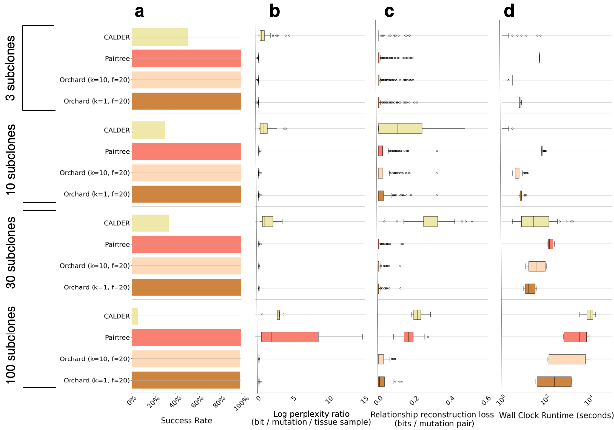
Figure 5: Benchmark performance on 576 simulated data sets used previously in [24]. The simulation results are grouped by the number of subclones (rows), and these groups are referred to as a problem size. A. Bar plots show the success rate for each method on a problem size. A method is successful on a reconstruction problem if it produces at least one valid tree. The distributions in b-d only reflect data sets where a method was successful. B. Box plots show the distribution of log perplexity ratio for each method on a problem size. Log perplexity ratio is reported relative to the true mutation frequency matrix $F^{(\text{true})}$ used to generate the VAF data, and therefore can be negative. C. The distribution of relationship reconstruction loss for each method on a problem size. D. The distributions of wall clock run time in seconds.

A.10.2 Results on 3 chronic lymphocytic leukemias (CLLs)

In this section, we show the results comparing Orchard, Pairtree, and CALDER on 3 chronic lymphocytic leukemia (CLL) data sets originally from [14]. The CLL data sets consist of varying numbers of subclones (either 4 or 5), tissue samples (5), and mutations (between 11 and 20). All of the CLL data sets had an approximate sequencing depth of 40x [14]. The mutation clusters for these data sets were inferred using a k-means algorithm, and then clone trees were derived by experts using these clusters.

The results in Figure 6 show that Orchard, Pairtree, and CALDER succeeded on all 3 CLL data sets. Pairtree and Orchard have nearly identical performance for log perplexity ratio, while both of Orchard’s configurations are about 10x faster than Pairtree. CALDER had a higher log perplexity ratio than Pairtree and Orchard on all 3 CLL data sets, but was about 10x faster than Orchard and about 100x faster than Pairtree.

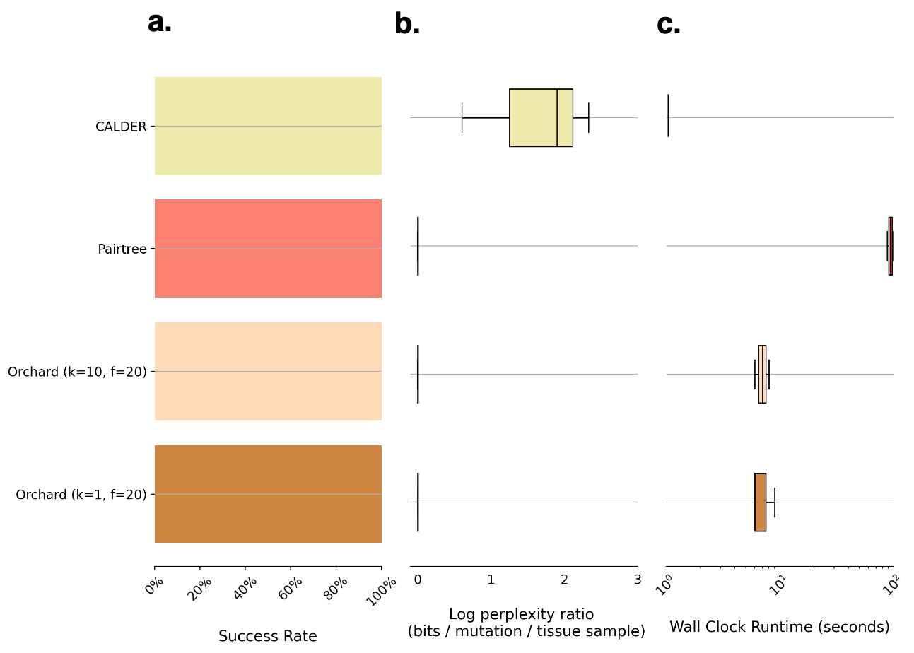
Figure 6: Reconstruction performance of Orchard, CALDER [25] and Pairtree [24] on 3 chronic lymphocytic leukemia (CLL) data sets originally from [14]. a. Orchard, CALDER, and Pairtree succeeded on all 3 CLL data sets. b. The distribution of log perplexity ratio for each method on the 3 CLL data sets. The log perplexity ratio measures the average per-mutation decrease in log-likelihood of the VAF data using the mutation frequency matrix ($F$) recovered by a method, relative to the perplexity of the maximum a posteriori (MAP) mutation frequency $F^{(\text{MAP})}$ fit to the expert-derived trees. c. The distributions of wall clock run time in seconds.

A.10.3 Comparing expert-derived trees to those inferred using ’phylogeny-aware’ clustering

In Section 2.3.4, we compared our phylogeny-aware clustering method to state-of-the-art VAF based clustering methods [28, 27, 26] on 14 B-ALL datasets originally from [39]. Our ’ground truth’ for these clustering results are expert-derived mutation clusterings from [39]. We now will use the clustering results from Section 2.3.4 to construct clone trees, and then compare those clone trees to the expert-derived clone trees for the 14 B-ALL data sets. To make our comparison more fair, we chose to make sure the trees compared contain the same number of nodes. Since the mutation clustering algorithms PyClone-VI [27], VIBER [26], and SciClone [28] can yield clusterings with varying numbers of clusters for the same data set, it’s difficult to compare trees constructed on these mutation clusterings directly to each other or to the expert-derived trees unless they all contain the same number of clusters. In fact, there is not a single instance where all of these methods found the same number of clusters for any of the 14 B-ALL data sets. On the other hand, our phylogeny-aware clustering algorithm allows the user to manually select a tree of any size (i.e., one with a particular number of clones). Therefore, it’s very easy to select the tree inferred by our phylogeny-aware clustering algorithm that has the same number of nodes as the expert-derived tree for a data set.

Figure 7 shows the log perplexity ratio of the correct size tree (in reference to the expert-derived trees) inferred by our phylogeny-aware clustering method (Orchard+Cluster), i.e., we ran phylogeny-aware clustering on the mutation trees outputted by Orchard with $k=10$, and selected the inferred clone tree that has the same number of nodes as the expert-derived tree. For 2/14 data sets, our phylogeny-aware clustering method had a lower perplexity compared to the baseline (SVJET010, and SJBALL031). The two B-ALL data sets identified as outliers in Figure 7 were SJBALL022610 (+6.19 bits compared to baseline) and SJMLL039 (+2.15 bits compared to baseline). On the remaining 10 B-ALL data sets, our phylogeny-aware clustering method nearly matched the expert-derived trees where it had on average +0.05 bits. It’s important to note that the data set SJBALL022610 has the highest number of mutation (292), and the clustering results for this data set shown in Figure 13 are poor. For the majority of B-ALL data sets, the clone trees inferred by the phylogeny-aware clustering algorithm have very similar perplexity to the MAP mutation frequency matrix $F^{(\text{MAP})}$ fit to the expert-derived clone trees.

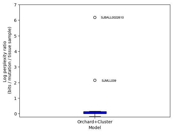
Figure 7: Box plots show the distribution of log perplexity ratio for the trees inferred by our ’phylogeny-aware’ clustering method (Orchard+Cluster) for the 14 B-ALL data sets from [39]. The log perplexity ratio measures the relative average per-mutation decrease in log likelihood of the VAF data using the mutation frequency matrix ($F$) recovered by the method, relative to the perplexity of the maximum a posterior (MAP) mutation frequency matrix $F^{(\text{MAP})}$ fit to expert-derived tree for each of the 14 B-ALL data sets.

A.10.4 Constructing clone trees on inferred mutation clusters versus inferring clone trees using ’phylogeny-aware’ clustering

To further evaluate our phylogeny-aware clustering algorithm, we decided to use Orchard and Pairtree to construct trees on the mutation clusters inferred by PyClone-VI in Section 2.3.4. We then use the number of clusters PyClone-VI inferred for each data set to manually select the same size tree inferred by our phylogeny-aware clustering method. Again, since we are unable to manually enforce a number of clusters for all methods shown in Figure 3, we chose to only compare against PyClone-VI because it had the best performance amongst all of the VAF based mutation clustering algorithms from our analysis in Section 2.3.4.

In Figure 8, we show the log perplexity of the trees constructed by Orchard $(k=10)$ and Pairtree using the mutation clusters inferred by PyClone-VI for each of the 14 B-ALL data sets, as well as the log perplexity of the same size tree inferred by our phylogeny-aware clustering algorithm. ’PyClone-VI+Pairtree’ refers to the trees constructed by Pairtree using the mutation clusters inferred by PyClone-VI. ’PyClone-VI+Orchard’ refers to the trees constructed by Orchard $(k=10)$ using the mutation clusters inferred by PyClone-VI. ’Orchard+Cluster’ refers to the clone trees inferred by our phylogeny-aware clustering algorithm using the mutation trees constructed by Orchard $(k=10)$. Generally, ’PyClone-VI+Pairtree’ and ’PyClone-VI+Orchard’ had nearly identical log perplexity across all 14 B-ALL data sets. On 3/14 B-ALL data sets, the tree inferred by our phylogeny-aware clustering algorithm had a lower log perplexity compared to the trees inferred by ’PyClone-VI+Pairtree’ and ’PyClone-VI+Orchard’ (avg. of -1.1e-4 bits). On the remaining 11 B-ALL data sets the clone trees inferred by our phylogeny-aware clustering method had significantly higher log perplexity (avg. of +4.4 bits).

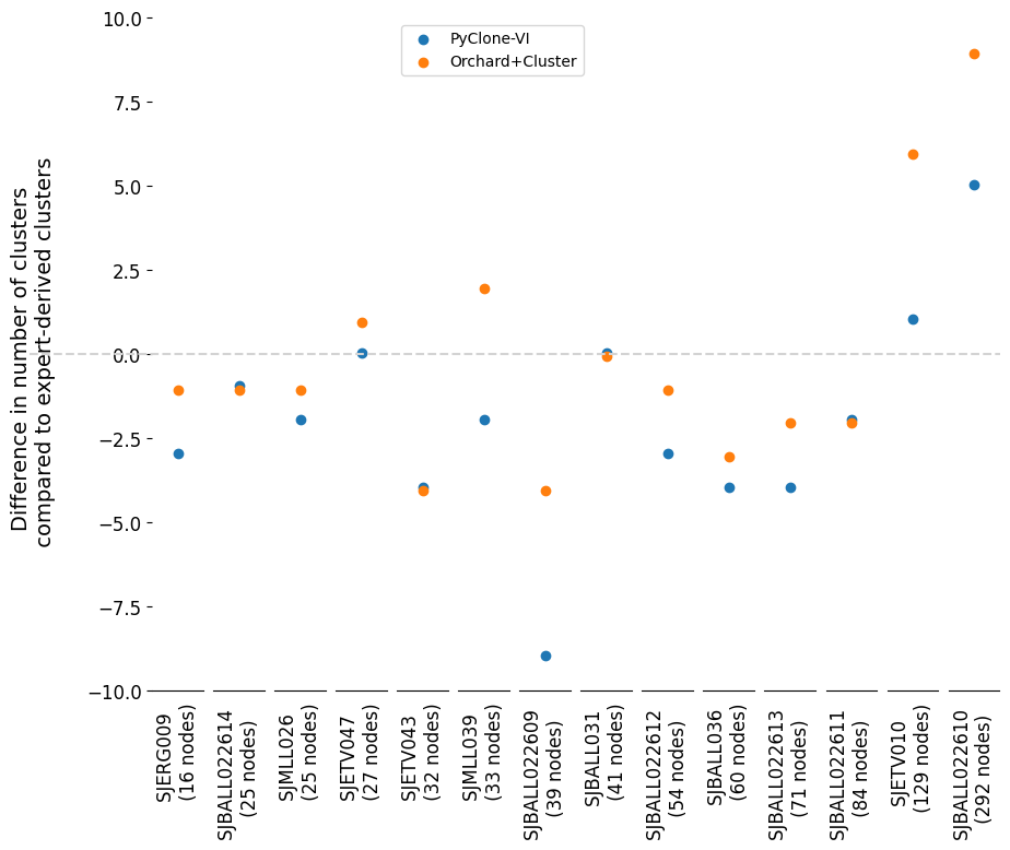
Figure 16: Difference in the number of clusters inferred by ’phylogeny-aware’ clustering and PyClone-VI [27] for each of the 14 B-ALL data sets from [39], relative to the number of clusters derived by experts. Each column shows the results for a single B-ALL data set. The horizontal gray dotted line represents no difference in the number of clusters inferred by a method compared to the number of clusters derived by experts. A point that lies far above or below this gray dotted line means that a method inferred a number of clusters for a B-ALL data set that is very different from the number of clusters derived by experts for that data set.

Although our phylogeny-aware clustering algorithm performs poorly in this analysis, we believe it’s largely due to the fact that PyClone-VI (and all of the VAF based clustering methods) infer clusterings on the B-ALL data sets that contain fewer clusters compared to the expert-derived clusterings. This is evident in the results shown in Figure 16. PyClone-VI in particular infers fewer clones than the expert-derived clusterings on 10/14 B-ALL datasets (avg. of 3.4 fewer clones per dataset). It’s clear from our results in Figure 7 that our phylogeny-aware clustering method performs well when the correct number of clones is chosen, and Figure 16 supports that our phylogeny-aware clustering algorithm converges more closely to the correct number of clusters. These results suggest that generally the number of clusters chosen by PyClone-VI is too few for the phylogeny-aware clustering algorithm to perform well, and that the phylogeny-aware clustering algorithm converged at a number of clusters that is closer to the number of clusters derived by experts.

Figure 8: Box plots show the distribution of log perplexity for the trees inferred by our ’phylogeny-aware’ clustering method (Orchard+Cluster), and the trees constructed by Orchard $(k=10)$ and Pairtree using the mutation clusters inferred by PyClone-VI [27] for the 14 B-ALL data sets from [39]. Generally, the clone trees inferred by the phylogeny-aware clustering algorithm (’Orchard+Cluster’) have a higher log perplexity (worse performance) than the clone trees of the same size constructed by Pairtree or Orchard using the mutation clusters inferred by PyClone-VI. ’PyClone-VI+Pairtree’ refers to the trees constructed by Pairtree using the mutation clusters inferred by PyClone-VI. ’PyClone-VI+Orchard’ refers to the trees constructed by Orchard $(k=10)$ using the mutation clusters inferred by PyClone-VI. Log perplexity is not reported relative to a baseline, and therefore is always non-negative.

A.10.5 Comparing the $\widehat{F}$ sum node order to a random node ordering

In Figure 9, we compare the $\widehat{F}$ sum approach to a random node ordering approach on the 90 simulated mutation tree data sets. It’s clear from Figure 9a-b that randomizing the node order leads to slightly higher log perplexity ratio and slightly higher relationship reconstruction loss compared to using the $\widehat{F}$ sum node order. It’s also clear from Figure 9c that randomizing the node order leads to slightly longer run times. We believe the slight increase in run times using the randomized node order can be attributed to the projection algorithm [35] requiring more iterations to fit the clonal proportion matrix $U$; poor node placements requires the algorithm to adjust more values in $U$ in order to adhere to the perfect phylogeny constraints. As previously discussed in Section A.5.1, one possible reason that randomizing the node order leads to slightly worse reconstructions is that a node could be placed into the tree long before one or more of its ancestors is placed in the tree.

Although randomizing the node order results in slightly worse reconstructions, it’s also clear that using Orchard with a randomized node order will still produce significantly better trees on larger reconstruction problems (50+ nodes) compared to existing methods such as Pairtree [24] or CALDER [25]. These results also support that the node placement scoring function described in Section A.6 is robust to any node order.

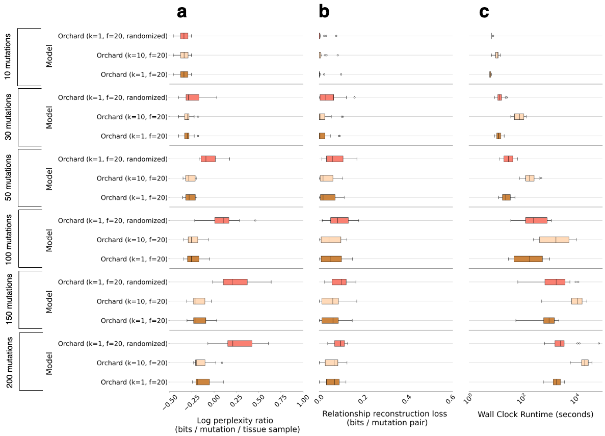
Figure 9: Comparison of Orchard using a randomized node order vs. Orchard using the $\widehat{F}$ sum node order on 90 simulated mutation tree data sets. The simulation results are grouped by the number of mutations (rows), and these groups are referred to as a problem size. These results show that using a randomized node order can result in slightly worse reconstructions compared to using the $\widehat{F}$ sum order described in A.5.2. a. The distribution of log perplexity ratio for each method on a problem size. Log perplexity ratio is reported relative to the true cellular prevalence matrix $F^{(\text{true})}$ used to generate the data, and therefore can be negative. b. The distribution of relationship reconstruction loss for each method on a problem size. c. The distributions of wall clock run time in seconds.

A.10.6 Comparing Orchard in its stochastic and deterministic modes

Orchard is made stochastic by using the Ancestral Gumbel-Max trick. If this trick is not used, Orchard can be run in a deterministic mode which we refer to as its beam search mode. Figure 10 compares Orchard in its stochastic mode (Orchard) versus its deterministic mode (Beam Search) on the 90 simulated mutation tree data sets.

Figure 10a-b shows that using the Ancestral Gumbel-Max trick decreases the variance of the log perplexity ratio and relationship reconstruction loss, and slightly improves reconstructions compared to Orchard in its deterministic mode (Beam Search). Figure 10c however shows that Orchard’s deterministic mode (Beam Search) is generally faster than Orchard’s stochastic mode on larger mutation tree reconstruction problems (100+ nodes). These results suggest that Orchard’s deterministic mode may be useful for performing large reconstructions quickly, but that the speed improvements come at a cost of potentially worse reconstructions.

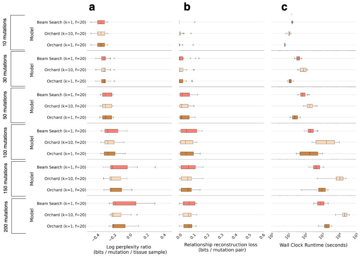
Figure 10: Comparing Orchard’s stochastic mode (Orchard) versus Orchard’s deterministic mode (Beam Search) on 90 simulated mutation tree data sets. The simulation results are grouped by the number of mutations (rows), and these groups are referred to as a problem size. These results show that using similar techniques to those described in [32, 33] for adding stochasticity to Orchard’s tree search generally decreases perplexity and relationship reconstruction loss compare to using a deterministic beam search. a. The distribution of log perplexity ratio for each method on a problem size. Log perplexity ratio is reported relative to the true cellular prevalence matrix $F^{(\text{true})}$ used to generate the data, and therefore can be negative. b. The distribution of relationship reconstruction loss for each method on a problem size. c. The distributions of wall clock run time in seconds.

A.10.7 Evaluating the phylogeny-aware clustering algorithm using simulated data

In this section, we evaluate the phylogeny-aware clustering algorithm using simulated cancer data. We used the Pearsim software (https://github.com/morrislab/pearsim) to simulate a total of 12 different simulated cancers each with 10 subclones, and 10 cancer samples. The data sets only varied in the number of mutations per subclone (10, 20, 100), and for each choice of mutations per subclone we simulated 4 different data sets at a 50x sequencing depth. By varying the number of mutations per subclone, the simulated data varies in the total number of mutations in each data set (100, 200, or 1000). This allows us to evaluate Orchard’s ability to reconstruct very large mutation trees (100, 200, or 1000 nodes), and then we can evaluate the phylogeny-aware clustering algorithm’s ability to infer subclones from these mutation trees. The subclones inferred by the phylogeny-aware clustering algorithm can then be compared to the ground-truth clusters for each simulated data set.

Figure 11a-b shows the distribution of log perplexity ratio and wall clock run time for the mutation trees reconstructed by Orchard ($k=1$) on the 12 simulated cancer data sets. Each row in Figure 11 shows the results on the data sets of a particular size (100, 200, or 1000 mutations). The log perplexity ratio is measured in reference to the mutation frequency matrix $F^{(\text{true})}$ used to generate the simulated clone trees and their associated VAF data. It’s clear that Orchard can reconstruct extremely large mutation trees that fit the VAF data equally as well the ground-truth mutation frequency matrix $F^{(\text{true})}$ used to generate the VAF data. It’s also clear from Figure 11b that the run times for Orchard can get quite large (24 hrs+) on mutation tree reconstruction problems with 1000 nodes.

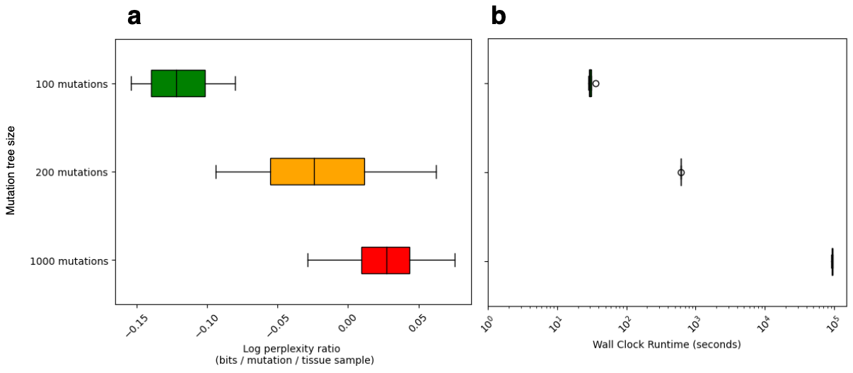
Figure 11: Box plots show the distribution of log perplexity ratio and wall clock run time for the trees inferred by Orchard ($k=1$) on the 12 simulated cancer data sets. The simulated results are grouped by the number of mutations in each data set (rows). a. The distribution of log perplexity ratio on each problem size. Log perplexity ratio is reported relative to the ground-truth mutation frequency matrix $F^{(\text{true})}$ used to generate the simulated VAF data, and therefore can be negative. b. The distributions of wall clock run time in seconds.

Figure 12a-b shows the evaluation result for the mutation clusters inferred by the phylogeny-aware clustering algorithm (’Orchard+Cluster’), VIBER [26], and PyClone-VI [27] on the 12 simulated cancer data sets. The results for ’Orchard+Cluster’ are computed from the mutation clusters inferred by the phylogeny-aware clustering algorithm using the mutation trees reconstructed by Orchard ($k=1$) that were evaluated in Figure 11. Figure 12a-b shows the distribution of Adjusted Rand Index and Normalized lineage count similarity for each clustering method on a problem size. It’s clear from the results shown in Figure 12 that the phylogeny-aware clustering algorithm can scale quite well to large clustering problems. Even on the 1000 mutation problems, the phylogeny-aware clustering was still competitive with the state-of-the-art VAF based clustering methods.

We performed similar experiments to evaluate the phylogeny-aware clustering algorithm on other simulated data, and the results generally agree with what’s shown in Figure 12. One area we found the phylogeny-aware clustering algorithm doesn’t perform as well is when the simulated data sets are very large (200+ mutations), and there are very few samples (3 or fewer). We do not believe the phylogeny-aware clustering algorithm will perform well for these types of problems. We believe this may be partly due to the fact that these are difficult mutation tree reconstruction problems, and if the reconstructed trees are inaccurate this may make it difficult for the phylogeny-aware clustering algorithm to infer plausible clusters.

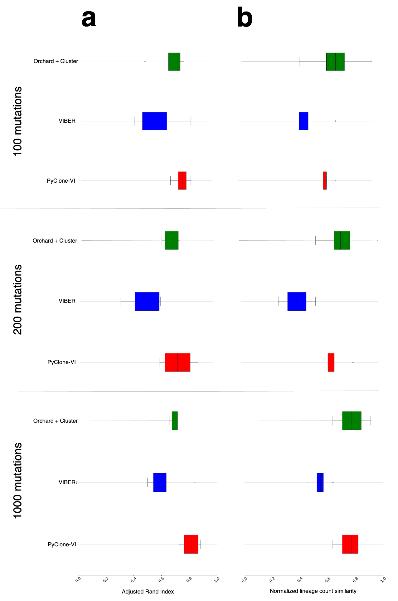
Figure 12: Evaluation of ’phylogeny-aware’ clustering versus state-of-the-art VAF-based mutation clustering methods on 12 simulated cancers. Each simulated data set contains 10 subclones, 10 cancer samples, and the VAF data has a sequencing depth of 50x. The data sets only vary in the number of mutations (100, 200, 1000). The Adjusted Rand Index, and normalized lineage count similarity are measured in reference to the ground-truth mutation clusters for each of the 12 simulated data sets. The results are grouped by the number of mutations in each data set (rows). a. Box plots show the distribution of the Adjusted Rand Index for each method. b. Box plots show the distribution of the normalized lineage count similarity for each method.

A.11 Supplemental Figures

Figure 13: Adjusted Rand Index (ARI) for the ’phylogeny-aware’ clustering algorithm and the VAF based mutation clustering algorithms on 14 B-ALL data sets. Each column shows the results for all methods on a single B-ALL data set. ARI is measured in reference to the expert-derived mutation clusters for the 14 B-ALL data sets. Bar plots show the ARI for each method on a data set.

Figure 14: Comparison of normalized lineage count similarity for the ’phylogeny-aware’ clustering algorithm and the VAF based mutation clustering algorithms on 14 B-ALL data sets. Each column shows the results for all methods on a single B-ALL data set. Normalized lineage count similarity is measured in reference to the expert-derived mutation clusters for the 14 B-ALL data sets. Bar plots show the normalized lineage count similarity for each method on a data set.

Figure 15: Bar plots show the log perplexity of the clone trees reconstructed by Orchard, Pairtree [24], and CALDER [25] on the 14 B-ALL data sets originally from [39]. Each column shows the log perplexity of the tree(s) reconstructed by a method for an individual B-ALL data set. A red $x$ in the location where the log perplexity should be for a method means the method did not succeed on that data set. CALDER failed on 2/14 data sets (SJERG009 and SJBALL022612), while Orchard and Pairtree succeed on all 14 data sets. A large log perplexity means that the tree(s) recovered by a method fit the VAF data poorly. Log perplexity is not reported relative to a baseline, and therefore is always non-negative. Pairtree and Orchard have similar levels of perplexity across all B-ALL data sets, while CALDER had the highest perplexity (worst performance) on the subset of data sets where it succeeded.

References

-
[1]
D. Hanahan, R. A. Weinberg, The Hallmarks of Cancer, Cell 100 (1) (2000) 57–70, number: 1 Publisher: Elsevier.
doi:10.1016/S0092-8674(00)81683-9.
URL https://www.cell.com/cell/abstract/S0092-8674(00)81683-9 - [2] P. C. Nowell, The clonal evolution of tumor cell populations, Science (New York, N.Y.) 194 (4260) (1976) 23–28, number: 4260. doi:10.1126/science.959840.
-
[3]
M. Greaves, C. C. Maley, Clonal evolution in cancer, Nature 481 (7381) (2012) 306–313, number: 7381 Publisher: Nature Publishing Group.
doi:10.1038/nature10762.
URL https://www.nature.com/articles/nature10762 -
[4]
M. Gerstung, C. Jolly, I. Leshchiner, S. C. Dentro, S. Gonzalez, D. Rosebrock, T. J. Mitchell, Y. Rubanova, P. Anur, K. Yu, M. Tarabichi, A. Deshwar, J. Wintersinger, K. Kleinheinz, I. Vázquez-García, K. Haase, L. Jerman, S. Sengupta, G. Macintyre, S. Malikic, N. Donmez, D. G. Livitz, M. Cmero, J. Demeulemeester, S. Schumacher, Y. Fan, X. Yao, J. Lee, M. Schlesner, P. C. Boutros, D. D. Bowtell, H. Zhu, G. Getz, M. Imielinski, R. Beroukhim, S. C. Sahinalp, Y. Ji, M. Peifer, F. Markowetz, V. Mustonen, K. Yuan, W. Wang, Q. D. Morris, P. T. Spellman, D. C. Wedge, P. Van Loo, The evolutionary history of 2,658 cancers, Nature 578 (7793) (2020) 122–128, number: 7793 Publisher: Nature Publishing Group.
doi:10.1038/s41586-019-1907-7.
URL https://www.nature.com/articles/s41586-019-1907-7 -
[5]
S. C. Dentro, I. Leshchiner, K. Haase, M. Tarabichi, J. Wintersinger, A. G. Deshwar, K. Yu, Y. Rubanova, G. Macintyre, J. Demeulemeester, I. Vázquez-García, K. Kleinheinz, D. G. Livitz, S. Malikic, N. Donmez, S. Sengupta, P. Anur, C. Jolly, M. Cmero, D. Rosebrock, S. E. Schumacher, Y. Fan, M. Fittall, R. M. Drews, X. Yao, T. B. K. Watkins, J. Lee, M. Schlesner, H. Zhu, D. J. Adams, N. McGranahan, C. Swanton, G. Getz, P. C. Boutros, M. Imielinski, R. Beroukhim, S. C. Sahinalp, Y. Ji, M. Peifer, I. Martincorena, F. Markowetz, V. Mustonen, K. Yuan, M. Gerstung, P. T. Spellman, W. Wang, Q. D. Morris, D. C. Wedge, P. Van Loo, S. C. Dentro, I. Leshchiner, M. Gerstung, C. Jolly, K. Haase, M. Tarabichi, J. Wintersinger, A. G. Deshwar, K. Yu, S. Gonzalez, Y. Rubanova, G. Macintyre, J. Demeulemeester, D. J. Adams, P. Anur, R. Beroukhim, P. C. Boutros, D. D. Bowtell, P. J. Campbell, S. Cao, E. L. Christie, M. Cmero, Y. Cun, K. J. Dawson, N. Donmez, R. M. Drews, R. Eils, Y. Fan, M. Fittall, D. W. Garsed, G. Getz,
G. Ha, M. Imielinski, L. Jerman, Y. Ji, K. Kleinheinz, J. Lee, H. Lee-Six, D. G. Livitz, S. Malikic, F. Markowetz, I. Martincorena, T. J. Mitchell, V. Mustonen, L. Oesper, M. Peifer, M. Peto, B. J. Raphael, D. Rosebrock, S. C. Sahinalp, A. Salcedo, M. Schlesner, S. E. Schumacher, S. Sengupta, R. Shi, S. J. Shin, L. D. Stein, O. Spiro, I. Vázquez-García, S. Vembu, D. A. Wheeler, T.-P. Yang, X. Yao, K. Yuan, H. Zhu, W. Wang, Q. D. Morris, P. T. Spellman, D. C. Wedge, P. Van Loo, Characterizing genetic intra-tumor heterogeneity across 2,658 human cancer genomes, Cell 184 (8) (2021) 2239–2254.e39, number: 8.
doi:10.1016/j.cell.2021.03.009.
URL https://www.sciencedirect.com/science/article/pii/S0092867421002944 -
[6]
D. G. Kent, A. R. Green, Order Matters: The Order of Somatic Mutations Influences Cancer Evolution, Cold Spring Harbor Perspectives in Medicine 7 (4) (2017) a027060, number: 4.
doi:10.1101/cshperspect.a027060.
URL https://www.ncbi.nlm.nih.gov/pmc/articles/PMC5378012/ -
[7]
L. Koch, Using tumour phylogenies to identify drivers, Nature Reviews Genetics 23 (4) (2022) 196–196, number: 4 Publisher: Nature Publishing Group.
doi:10.1038/s41576-022-00458-9.
URL https://www.nature.com/articles/s41576-022-00458-9 - [8] K. L. Pogrebniak, C. Curtis, Harnessing Tumor Evolution to Circumvent Resistance, Trends in genetics: TIG 34 (8) (2018) 639–651, number: 8. doi:10.1016/j.tig.2018.05.007.
-
[9]
E. N. Adams, Consensus Techniques and the Comparison of Taxonomic Trees, Systematic Zoology 21 (4) (1972) 390–397, number: 4 Publisher: [Oxford University Press, Society of Systematic Biologists, Taylor & Francis, Ltd.].
doi:10.2307/2412432.
URL https://www.jstor.org/stable/2412432 - [10] S. Nik-Zainal, P. Van Loo, D. C. Wedge, L. B. Alexandrov, C. D. Greenman, K. W. Lau, K. Raine, D. Jones, J. Marshall, M. Ramakrishna, A. Shlien, S. L. Cooke, J. Hinton, A. Menzies, L. A. Stebbings, C. Leroy, M. Jia, R. Rance, L. J. Mudie, S. J. Gamble, P. J. Stephens, S. McLaren, P. S. Tarpey, E. Papaemmanuil, H. R. Davies, I. Varela, D. J. McBride, G. R. Bignell, K. Leung, A. P. Butler, J. W. Teague, S. Martin, G. Jönsson, O. Mariani, S. Boyault, P. Miron, A. Fatima, A. Langerød, S. A. J. R. Aparicio, A. Tutt, A. M. Sieuwerts, A. Borg, G. Thomas, A. V. Salomon, A. L. Richardson, A.-L. Børresen-Dale, P. A. Futreal, M. R. Stratton, P. J. Campbell, Breast Cancer Working Group of the International Cancer Genome Consortium, The life history of 21 breast cancers, Cell 149 (5) (2012) 994–1007, number: 5. doi:10.1016/j.cell.2012.04.023.
-
[11]
M. Jamal-Hanjani, G. A. Wilson, N. McGranahan, N. J. Birkbak, T. B. Watkins, S. Veeriah, S. Shafi, D. H. Johnson, R. Mitter, R. Rosenthal, M. Salm, S. Horswell, M. Escudero, N. Matthews, A. Rowan, T. Chambers, D. A. Moore, S. Turajlic, H. Xu, S.-M. Lee, M. D. Forster, T. Ahmad, C. T. Hiley, C. Abbosh, M. Falzon, E. Borg, T. Marafioti, D. Lawrence, M. Hayward, S. Kolvekar, N. Panagiotopoulos, S. M. Janes, R. Thakrar, A. Ahmed, F. Blackhall, Y. Summers, R. Shah, L. Joseph, A. M. Quinn, P. A. Crosbie, B. Naidu, G. Middleton, G. Langman, S. Trotter, M. Nicolson, H. Remmen, K. Kerr, M. Chetty, L. Gomersall, D. A. Fennell, A. Nakas, S. Rathinam, G. Anand, S. Khan, P. Russell, V. Ezhil, B. Ismail, M. Irvin-Sellers, V. Prakash, J. F. Lester, M. Kornaszewska, R. Attanoos, H. Adams, H. Davies, S. Dentro, P. Taniere, B. O’Sullivan, H. L. Lowe, J. A. Hartley, N. Iles, H. Bell, Y. Ngai, J. A. Shaw, J. Herrero, Z. Szallasi, R. F. Schwarz, A. Stewart, S. A. Quezada, J. Le Quesne, P. Van Loo, C. Dive, A. Hackshaw,
C. Swanton, Tracking the Evolution of Non–Small-Cell Lung Cancer, New England Journal of Medicine 376 (22) (2017) 2109–2121, number: 22 Publisher: Massachusetts Medical Society _eprint: https://doi.org/10.1056/NEJMoa1616288.
doi:10.1056/NEJMoa1616288.
URL https://doi.org/10.1056/NEJMoa1616288 -
[12]
N. Light, M. Layeghifard, A. Attery, V. Subasri, M. Zatzman, N. D. Anderson, R. Hatkar, S. Blay, D. Chen, A. Novokmet, F. Fuligni, J. Tran, R. de Borja, H. Agarwal, L. Waldman, L. M. Abegglen, D. Albertson, J. L. Finlay, J. R. Hansford, S. Behjati, A. Villani, M. Gerstung, L. B. Alexandrov, G. R. Somers, J. D. Schiffman, V. Rotter, D. Malkin, A. Shlien, Germline TP53 mutations undergo copy number gain years prior to tumor diagnosis, Nature Communications 14 (1) (2023) 77, number: 1 Publisher: Nature Publishing Group.
doi:10.1038/s41467-022-35727-y.
URL https://www.nature.com/articles/s41467-022-35727-y - [13] H. Sakamoto, M. A. Attiyeh, J. M. Gerold, A. P. Makohon-Moore, A. Hayashi, J. Hong, R. Kappagantula, L. Zhang, J. P. Melchor, J. G. Reiter, A. Heyde, C. M. Bielski, A. V. Penson, M. Gönen, D. Chakravarty, E. M. O’Reilly, L. D. Wood, R. H. Hruban, M. A. Nowak, N. D. Socci, B. S. Taylor, C. A. Iacobuzio-Donahue, The Evolutionary Origins of Recurrent Pancreatic Cancer, Cancer Discovery 10 (6) (2020) 792–805, number: 6. doi:10.1158/2159-8290.CD-19-1508.
-
[14]
A. Schuh, J. Becq, S. Humphray, A. Alexa, A. Burns, R. Clifford, S. M. Feller, R. Grocock, S. Henderson, I. Khrebtukova, Z. Kingsbury, S. Luo, D. McBride, L. Murray, T. Menju, A. Timbs, M. Ross, J. Taylor, D. Bentley, Monitoring chronic lymphocytic leukemia progression by whole genome sequencing reveals heterogeneous clonal evolution patterns, Blood 120 (20) (2012) 4191–4196, number: 20.
doi:10.1182/blood-2012-05-433540.
URL https://doi.org/10.1182/blood-2012-05-433540 -
[15]
A. Villani, S. Davidson, N. Kanwar, W. W. Lo, Y. Li, S. Cohen-Gogo, F. Fuligni, L.-M. Edward, N. Light, M. Layeghifard, R. Harripaul, L. Waldman, B. Gallinger, F. Comitani, L. Brunga, R. Hayes, N. D. Anderson, A. K. Ramani, K. E. Yuki, S. Blay, B. Johnstone, C. Inglese, R. Hammad, C. Goudie, A. Shuen, J. D. Wasserman, R. E. Venier, M. Eliou, M. Lorenti, C. A. Ryan, M. Braga, M. Gloven-Brown, J. Han, M. Montero, F. Spatare, J. A. Whitlock, S. W. Scherer, K. Chun, M. J. Somerville, C. Hawkins, M. Abdelhaleem, V. Ramaswamy, G. R. Somers, L. Kyriakopoulou, J. Hitzler, M. Shago, D. A. Morgenstern, U. Tabori, S. Meyn, M. S. Irwin, D. Malkin, A. Shlien, The clinical utility of integrative genomics in childhood cancer extends beyond targetable mutations, Nature Cancer (2022) 1–19Publisher: Nature Publishing Group.
doi:10.1038/s43018-022-00474-y.
URL https://www.nature.com/articles/s43018-022-00474-y -
[16]
M. El-Kebir, G. Satas, B. J. Raphael, Inferring parsimonious migration histories for metastatic cancers, Nature Genetics 50 (5) (2018) 718–726, number: 5 Publisher: Nature Publishing Group.
doi:10.1038/s41588-018-0106-z.
URL https://www.nature.com/articles/s41588-018-0106-z -
[17]
S. Turajlic, H. Xu, K. Litchfield, A. Rowan, S. Horswell, T. Chambers, T. O’Brien, J. I. Lopez, T. B. Watkins, D. Nicol, M. Stares, B. Challacombe, S. Hazell, A. Chandra, T. J. Mitchell, L. Au, C. Eichler-Jonsson, F. Jabbar, A. Soultati, S. Chowdhury, S. Rudman, J. Lynch, A. Fernando, G. Stamp, E. Nye, A. Stewart, W. Xing, J. C. Smith, M. Escudero, A. Huffman, N. Matthews, G. Elgar, B. Phillimore, M. Costa, S. Begum, S. Ward, M. Salm, S. Boeing, R. Fisher, L. Spain, C. Navas, E. Grönroos, S. Hobor, S. Sharma, I. Aurangzeb, S. Lall, A. Polson, M. Varia, C. Horsfield, N. Fotiadis, L. Pickering, R. F. Schwarz, B. Silva, J. Herrero, N. M. Luscombe, M. Jamal-Hanjani, R. Rosenthal, N. J. Birkbak, G. A. Wilson, O. Pipek, D. Ribli, M. Krzystanek, I. Csabai, Z. Szallasi, M. Gore, N. McGranahan, P. Van Loo, P. Campbell, J. Larkin, C. Swanton, Deterministic Evolutionary Trajectories Influence Primary Tumor Growth: TRACERx Renal, Cell
173 (3) (2018) 595–610.e11, number: 3.
doi:10.1016/j.cell.2018.03.043.
URL https://www.ncbi.nlm.nih.gov/pmc/articles/PMC5938372/ -
[18]
Z. R. Chalmers, C. F. Connelly, D. Fabrizio, L. Gay, S. M. Ali, R. Ennis, A. Schrock, B. Campbell, A. Shlien, J. Chmielecki, F. Huang, Y. He, J. Sun, U. Tabori, M. Kennedy, D. S. Lieber, S. Roels, J. White, G. A. Otto, J. S. Ross, L. Garraway, V. A. Miller, P. J. Stephens, G. M. Frampton, Analysis of 100,000 human cancer genomes reveals the landscape of tumor mutational burden, Genome Medicine 9 (1) (2017) 34.
doi:10.1186/s13073-017-0424-2.
URL https://doi.org/10.1186/s13073-017-0424-2 -
[19]
D. Gusfield, Efficient algorithms for inferring evolutionary trees, Networks 21 (1) (1991) 19–28, number: 1 _eprint: https://onlinelibrary.wiley.com/doi/pdf/10.1002/net.3230210104.
doi:10.1002/net.3230210104.
URL https://onlinelibrary.wiley.com/doi/abs/10.1002/net.3230210104 -
[20]
M. El-Kebir, L. Oesper, H. Acheson-Field, B. J. Raphael, Reconstruction of clonal trees and tumor composition from multi-sample sequencing data, Bioinformatics 31 (12) (2015) i62–i70, number: 12.
doi:10.1093/bioinformatics/btv261.
URL https://doi.org/10.1093/bioinformatics/btv261 -
[21]
L. K. Sundermann, J. Wintersinger, G. Rätsch, J. Stoye, Q. Morris, Reconstructing tumor evolutionary histories and clone trees in polynomial-time with SubMARine, PLOS Computational Biology 17 (1) (2021) e1008400, number: 1 Publisher: Public Library of Science.
doi:10.1371/journal.pcbi.1008400.
URL https://journals.plos.org/ploscompbiol/article?id=10.1371/journal.pcbi.1008400 - [22] E. Eskin, E. Halperin, R. M. Karp, Efficient reconstruction of haplotype structure via perfect phylogeny, Journal of Bioinformatics and Computational Biology 1 (1) (2003) 1–20, number: 1. doi:10.1142/s0219720003000174.
-
[23]
D. Gusfield, Haplotyping as perfect phylogeny: conceptual framework and efficient solutions, in: Proceedings of the sixth annual international conference on Computational biology, RECOMB ’02, Association for Computing Machinery, New York, NY, USA, 2002, pp. 166–175.
doi:10.1145/565196.565218.
URL https://doi.org/10.1145/565196.565218 -
[24]
J. A. Wintersinger, S. M. Dobson, E. Kulman, L. D. Stein, J. E. Dick, Q. Morris, Reconstructing Complex Cancer Evolutionary Histories from Multiple Bulk DNA Samples Using Pairtree, Blood Cancer Discovery 3 (3) (2022) 208–219, number: 3.
doi:10.1158/2643-3230.BCD-21-0092.
URL https://doi.org/10.1158/2643-3230.BCD-21-0092 - [25] M. A. Myers, G. Satas, B. J. Raphael, CALDER: Inferring Phylogenetic Trees from Longitudinal Tumor Samples, Cell Systems 8 (6) (2019) 514–522.e5, number: 6. doi:10.1016/j.cels.2019.05.010.
-
[26]
G. Caravagna, T. Heide, M. J. Williams, L. Zapata, D. Nichol, K. Chkhaidze, W. Cross, G. D. Cresswell, B. Werner, A. Acar, L. Chesler, C. P. Barnes, G. Sanguinetti, T. A. Graham, A. Sottoriva, Subclonal reconstruction of tumors by using machine learning and population genetics, Nature Genetics 52 (9) (2020) 898–907, number: 9 Publisher: Nature Publishing Group.
doi:10.1038/s41588-020-0675-5.
URL https://www.nature.com/articles/s41588-020-0675-5 -
[27]
S. Gillis, A. Roth, PyClone-VI: scalable inference of clonal population structures using whole genome data, BMC Bioinformatics 21 (1) (2020) 571, number: 1.
doi:10.1186/s12859-020-03919-2.
URL https://doi.org/10.1186/s12859-020-03919-2 -
[28]
C. A. Miller, B. S. White, N. D. Dees, M. Griffith, J. S. Welch, O. L. Griffith, R. Vij, M. H. Tomasson, T. A. Graubert, M. J. Walter, M. J. Ellis, W. Schierding, J. F. DiPersio, T. J. Ley, E. R. Mardis, R. K. Wilson, L. Ding, SciClone: Inferring Clonal Architecture and Tracking the Spatial and Temporal Patterns of Tumor Evolution, PLOS Computational Biology 10 (8) (2014) e1003665, number: 8 Publisher: Public Library of Science.
doi:10.1371/journal.pcbi.1003665.
URL https://journals.plos.org/ploscompbiol/article?id=10.1371/journal.pcbi.1003665 -
[29]
A. Salcedo, M. Tarabichi, S. M. G. Espiritu, A. G. Deshwar, M. David, N. M. Wilson, S. Dentro, J. A. Wintersinger, L. Y. Liu, M. Ko, S. Sivanandan, H. Zhang, K. Zhu, T.-H. Ou Yang, J. M. Chilton, A. Buchanan, C. M. Lalansingh, C. P’ng, C. V. Anghel, I. Umar, B. Lo, W. Zou, J. T. Simpson, J. M. Stuart, D. Anastassiou, Y. Guan, A. D. Ewing, K. Ellrott, D. C. Wedge, Q. Morris, P. Van Loo, P. C. Boutros, A community effort to create standards for evaluating tumor subclonal reconstruction, Nature Biotechnology 38 (1) (2020) 97–107, number: 1 Publisher: Nature Publishing Group.
doi:10.1038/s41587-019-0364-z.
URL https://www.nature.com/articles/s41587-019-0364-z -
[30]
R. Sun, Z. Hu, A. Sottoriva, T. A. Graham, A. Harpak, Z. Ma, J. M. Fischer, D. Shibata, C. Curtis, Between-region genetic divergence reflects the mode and tempo of tumor evolution, Nature Genetics 49 (7) (2017) 1015–1024, number: 7 Publisher: Nature Publishing Group.
doi:10.1038/ng.3891.
URL https://www.nature.com/articles/ng.3891 -
[31]
M. J. Williams, B. Werner, C. P. Barnes, T. A. Graham, A. Sottoriva, Identification of neutral tumor evolution across cancer types, Nature Genetics 48 (3) (2016) 238–244, number: 3 Publisher: Nature Publishing Group.
doi:10.1038/ng.3489.
URL https://www.nature.com/articles/ng.3489 -
[32]
W. Kool, H. v. Hoof, M. Welling, Ancestral Gumbel-Top-k Sampling for Sampling Without Replacement, Journal of Machine Learning Research 21 (47) (2020) 1–36, number: 47.
URL http://jmlr.org/papers/v21/19-985.html -
[33]
W. Kool, H. van Hoof, M. Welling, Stochastic Beams and Where to Find Them: The Gumbel-Top-k Trick for Sampling Sequences Without Replacement, issue: arXiv:1903.06059 arXiv:1903.06059 [cs, stat] (May 2019).
URL http://arxiv.org/abs/1903.06059 -
[34]
M. Tarabichi, A. Salcedo, A. G. Deshwar, M. Ni Leathlobhair, J. Wintersinger, D. C. Wedge, P. Van Loo, Q. D. Morris, P. C. Boutros, A practical guide to cancer subclonal reconstruction from DNA sequencing, Nature Methods 18 (2) (2021) 144–155, number: 2 Publisher: Nature Publishing Group.
doi:10.1038/s41592-020-01013-2.
URL https://www.nature.com/articles/s41592-020-01013-2 -
[35]
B. Jia, S. Ray, S. Safavi, J. Bento, Efficient Projection onto the Perfect Phylogeny Model, in: Advances in Neural Information Processing Systems, Vol. 31, Curran Associates, Inc., 2018.
URL https://proceedings.neurips.cc/paper/2018/hash/d198bd736a97e7cecfdf8f4f2027ef80-Abstract.html -
[36]
S. Ray, B. Jia, S. Safavi, T. van Opijnen, R. Isberg, J. Rosch, J. Bento, Exact inference under the perfect phylogeny model, issue: arXiv:1908.08623 arXiv:1908.08623 [cs, q-bio] (Aug. 2019).
doi:10.48550/arXiv.1908.08623.
URL http://arxiv.org/abs/1908.08623 -
[37]
E. J. Gumbel, Statistical Theory of Extreme Values and Some Practical Applications. A Series of Lectures., Tech. Rep. PB175818, National Bureau of Standards, Washington, D. C. Applied Mathematics Div., issue: PB175818 Num Pages: 60 (1954).
URL https://ntrl.ntis.gov/NTRL/dashboard/searchResults/titleDetail/PB175818.xhtml -
[38]
M. B. Paulus, D. Choi, D. Tarlow, A. Krause, C. J. Maddison, Gradient Estimation with Stochastic Softmax Tricks, arXiv:2006.08063 [cs, stat] (Feb. 2021).
doi:10.48550/arXiv.2006.08063.
URL http://arxiv.org/abs/2006.08063 -
[39]
S. M. Dobson, L. García-Prat, R. J. Vanner, J. Wintersinger, E. Waanders, Z. Gu, J. McLeod, O. I. Gan, I. Grandal, D. Payne-Turner, M. N. Edmonson, X. Ma, Y. Fan, V. Voisin, M. Chan-Seng-Yue, S. Z. Xie, M. Hosseini, S. Abelson, P. Gupta, M. Rusch, Y. Shao, S. R. Olsen, G. Neale, S. M. Chan, G. Bader, J. Easton, C. J. Guidos, J. S. Danska, J. Zhang, M. D. Minden, Q. Morris, C. G. Mullighan, J. E. Dick, Relapse-Fated Latent Diagnosis Subclones in Acute B Lineage Leukemia Are Drug Tolerant and Possess Distinct Metabolic Programs, Cancer Discovery 10 (4) (2020) 568–587, number: 4.
doi:10.1158/2159-8290.CD-19-1059.
URL https://doi.org/10.1158/2159-8290.CD-19-1059 - [40] Y. Kim, S. Kwon, H. Choi, Consistent Model Selection Criteria on High Dimensions.
- [41] J. M. Santos, M. Embrechts, On the Use of the Adjusted Rand Index as a Metric for Evaluating Supervised Classification, in: C. Alippi, M. Polycarpou, C. Panayiotou, G. Ellinas (Eds.), Artificial Neural Networks – ICANN 2009, Lecture Notes in Computer Science, Springer, Berlin, Heidelberg, 2009, pp. 175–184. doi:10.1007/978-3-642-04277-5_18.
-
[42]
J. Ahrenfeldt, M. Waisi, I. C. Loft, P. T. L. C. Clausen, R. Allesøe, J. Szarvas, R. S. Hendriksen, F. M. Aarestrup, O. Lund, Metaphylogenetic analysis of global sewage reveals that bacterial strains associated with human disease show less degree of geographic clustering, Scientific Reports 10 (1) (2020) 3033, number: 1 Publisher: Nature Publishing Group.
doi:10.1038/s41598-020-59292-w.
URL https://www.nature.com/articles/s41598-020-59292-w -
[43]
E. Kulman, J. Wintersinger, Q. Morris, Reconstructing cancer phylogenies using Pairtree, a clone tree reconstruction algorithm, STAR Protocols 3 (4) (2022) 101706, number: 4.
doi:10.1016/j.xpro.2022.101706.
URL https://www.sciencedirect.com/science/article/pii/S266616672200586X -
[44]
A. K. Moretti, L. Zhang, C. A. Naesseth, H. Venner, D. Blei, I. Pe’er, variational combinatorial sequential monte carlo methods for bayesian phylogenetic inference, in: Proceedings of the Thirty-Seventh Conference on Uncertainty in Artificial Intelligence, PMLR, 2021, pp. 971–981, iSSN: 2640-3498.
URL https://proceedings.mlr.press/v161/moretti21a.html -
[45]
D. Müllner, Modern hierarchical, agglomerative clustering algorithms, issue: arXiv:1109.2378 arXiv:1109.2378 [cs, stat] (Sep. 2011).
doi:10.48550/arXiv.1109.2378.
URL http://arxiv.org/abs/1109.2378 -
[46]
A. A. Neath, J. E. Cavanaugh, The Bayesian information criterion: background, derivation, and applications, WIREs Computational Statistics 4 (2) (2012) 199–203, number: 2 _eprint: https://onlinelibrary.wiley.com/doi/pdf/10.1002/wics.199.
doi:10.1002/wics.199.
URL https://onlinelibrary.wiley.com/doi/abs/10.1002/wics.199