LLVM Static Analysis for Program Characterization and Memory Reuse Profile Estimation

Abstract

Profiling various application characteristics, including the number of different arithmetic operations performed, memory footprint, etc., dynamically is time- and space-consuming. On the other hand, static analysis methods, although fast, can be less accurate. This paper presents an LLVM-based probabilistic static analysis method that accurately predicts different program characteristics and estimates the reuse distance profile of a program by analyzing the LLVM IR file in constant time, regardless of program input size. We generate the basic-block-level control flow graph of the target application kernel and determine basic-block execution counts by solving the linear balance equation involving the adjacent basic blocks’ transition probabilities. Finally, we represent the kernel memory accesses in a bracketed format and employ a recursive algorithm to calculate the reuse distance profile. The results show that our approach can predict application characteristics accurately compared to another LLVM-based dynamic code analysis tool, Byfl.

Keywords: Reuse Distance Profile, LLVM Static Analysis, Static Trace, Probabilistic Cache Model, Control Flow Graph Analyzer

1 Introduction

With the help of advanced manufacturing and packaging techniques, complex CPUs contain billions of transistors condensed onto a single chip. Given their intricate nature, researchers must turn to performance modeling and program analysis tools to investigate the consequences of hardware design alterations, steering research in the correct direction. On the other hand, software developers can tune their software for particular hardware and conduct performance analysis using performance models. This approach also aids in selecting appropriate hardware for specific workloads. Consequently, program characterization and simulation tools facilitate hardware/software co-design.

A critical factor determining an application’s performance is the number and types of instructions it executes. Since each instruction is usually executed many times during a program execution, the number of times each execution provides insight into the application’s behavior. On the other hand, an application’s performance largely depends on the data availability to the arithmetic logic units. The cache utilization of an application and its data access pattern determines its locality.

In analyzing a cache’s performance, Reuse Distance Analysis [14] is one of the commonly used techniques [19, 20]. Reuse distance is defined as the number of unique memory references between two references to the same memory location. When a memory location is accessed for the first time, its reuse distance is infinite. The reuse profile is the histogram of reuse distances of all the memory accesses of a program. For sequential programs, the reuse profile is architecture-independent, needs to be calculated only once, and can be used to quickly predict memory performance while varying the cache architectural parameters. Although researchers tried to speed up reuse distance calculation by parallelizing the algorithm [16] and proposing analytical model and sampling techniques [8, 2], it still requires collecting a large amount of memory trace which is both time and space consuming. Recently, researchers proposed several methods to statically calculate reuse profile from source code [4, 7, 6, 15]. However, their approaches require modifying the programs or are limited to a single loop nest with numeric loop bounds.

This paper introduces an LLVM [12] static code analysis tool to gather program characteristics, including the number of different arithmetic operations, memory operations at both basic block and whole program level and the number of times each basic block is executed. It can also statically predict the reuse profile of the program without running the app or collecting the memory trace. It takes the source code and the branch probabilities as input and outputs different program statistics along with the reuse profile of the target kernel. Since we are interested in analyzing application kernels, our tool currently supports the reuse profile calculation of a single function. The prediction time of our model is input size invariant, making it highly scalable.

First, we dump the LLVM Intermediate Representation (IR) file using the Clang compiler. Then, we deploy an LLVM IR reader to read the IR file and generate a static application trace. We parse the static trace using the trace analyzer and generate the program’s Control Flow Graph (CFG). Each node in the CFG represents an LLVM basic block of the application. In this step, we also take the program branch probabilities for a specific input size to calculate the basic block execution counts and the number of different arithmetic/memory operations. We annotate CFG edges with branch probabilities and nodes with the execution counts and memory accesses. In the next step, we take the CFG as input, and using the branch probabilities and memory access information, we construct a loop annotated static memory trace of the program. Finally, we take the static memory trace and calculate the reuse profile using a recursive algorithm. We evaluate our analyzer with the program statistics collected from another LLVM binary instrumentation and code analysis tool, Byfl [17]. The results show that the model accurately predicts program characteristics and reuse profiles, given the same LLVM version used for Byfl and our static analyzer.

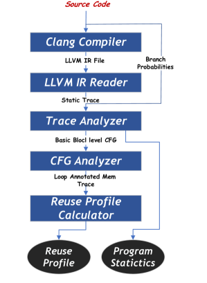
Figure 1: Overview of LLVM Static Analyzer

2 Related Work

Researchers investigated different approaches of static code analysis [10, 3, 11] and reuse profile calculation [4, 7, 6, 15].

Cousot et al. [9] described Astree, a static analyzer that provides runtime errors in C programs. However, they are bound to C program only, and their static analyzer cannot catch errors sometimes. Lindlan et al. [13], on the other hand, analyzes the Program Database Toolkit with both static and dynamic methods. Nevertheless, their static analysis needs an adequate front-end compilation. Bush et al. [5] describes a static compile-time analyzer that can detect various dynamic errors in some real-world programs. However, their static analysis approach is defined to some programs only.

Beyls et al. [17] proposed a method that highlights code areas with high reuse distances and then tries to refactor the code to reduce the cache misses. However, they are required to modify the source code. Narayanan et al. [15] proposed a static reuse distance-based memory model, but it is limited to loop-based programs. Cascaval et al. [6] presented a compile-time algorithm to compute reuse profile. However, they were also limited to loop-based programs and required program modification. Chauhan et al. [7] statically calculated reuse distance only for Matlab programs.

In contrast, our approach is probabilistic and leverages the LLVM IR to compute the reuse profiles and other program metrics. As a result, it enables us to support a variety of programming languages supported by LLVM compiler infrastructure. It also generates accurate profiles without changing the source program, and the output is tested with state-of-the-art dynamic models.

3 Methodology

In this section, we discuss our static analysis tool in detail. Figure 1 shows different steps of the analyzer where it shows that we collect various program characteristics at an early stage of the analyzer. Further, we extend it to calculate the reuse profile to predict cache hit rates. In the following sections, we discuss these steps in detail. In the following sections, we will use the program in Figure 2 as a running example.

3.1 Genarate LLVM IR File

In the first step, we generate the LLVM IR of the target program using the ‘clang -g -c -emit-llvm example.c’ command. Here, command line options enable ‘source-level debug information generation,’ ‘only preprocess, compile, and assemble steps,’ and ‘LLVM IR file generation’ options respective to their appearance. Thus, clang only runs ‘preprocess’ and ‘compilation’ steps while generating the IR with source-level debug information.

⬇

1int main() {

2 unsigned i, j, k, result, A = 10, arr[100][200];

3 for (i = 0; i < 100; i++) {

4 result += i;

5 for (j = 0; j < 200; j++) {

6 result = result * j + A;

7 for (k = 0; k < 300; k++)

8 result += k * k;

9 arr[i][j] = result;

10 }

11 }

12 return 0;

13}

Figure 2: Running example program.

3.2 LLVM IR File Reader

The second step of the static analyzer is the LLVM Intermediate Representation (IR) reader written as an LLVM pass. The reader takes the IR and optionally function name as input and outputs a static trace of the target function. It is written as an LLVM pass and uses LLVM compiler APIs to go over all the modules, functions, basic blocks, and instructions in the IR file.

Figure 3 shows a portion of the trace generated by the IR reader for the example program. Here, under ‘Example’ module, there is ‘main’ function. It receives no argument and consists of several basic blocks (‘e.g., entry, for.cond, for.body’). All the instructions under each basic block are also listed along with their position in the source ‘C’ program, operand list, and their types. For example, instruction ‘load’ in line 16 accesses ‘i’, where ‘i’ is loaded from memory, compared against 100 (line 18), and upon comparison, a branch is taken (line 21 in the trace). Thus, we can determine the variables accessed by each memory operation (load/store) within a basic block. In the case of array references (if the reference results from GEP instruction), we determine the index variables. For ‘loops’, we determine the loop control variable.

⬇

1Module : Example.llvm

2 Function <@ 0x7d8a88> : main : Definition : NonIntrinsic

3 ArgList :

4 BasicBlock <@ 0x7f3bd0> : entry

5 Instruction <@ 0x7f3d38> : (0, 0) : alloca

6 i32 : i32 1<@ 0x7f4390>

7 ............

8 ............

9 Instruction <@ 0x7f7130> : (4, 12) : store

10 i32 : i32 0<@ 0x7f4660>

11 i32* : i<@ 0x7f43f8>

12 Instruction <@ 0x7f7358> : (4, 10) : br

13 label : for.cond<@ 0x7f7290>

14

15 BasicBlock <@ 0x7f7290> : for.cond

16 Instruction <@ 0x7f72f8> : (4, 17) : load

17 i32* : i<@ 0x7f43f8>

18 Instruction <@ 0x7f7680> : (4, 19) : icmp

19 i32 : i32 %0<@ 0x7f72f8>

20 i32 : i32 100<@ 0x7f7620>

21 Instruction <@ 0x7f7a18> : (4, 5) : br

22 i1 : cmp<@ 0x7f7680>

23 label : for.end15<@ 0x7f78f0>

24 label : for.body<@ 0x7f7810>

25

26 BasicBlock <@ 0x7f7810> : for.body

27 Instruction <@ 0x7f7cf8> : (6, 16) : load

28 i32* : result<@ 0x7f4578>

29 ............

Figure 3: Portions of the static trace generated by parsing example program’s IR in Figure 2.

3.3 Trace Analyzer

The task of the trace analyzer can be divided into two steps. The steps are CFG generation and basic block count calculation.

A) Control Flow Graph Generation : We take the static trace as input and generate CFG of the target function in dot format. The CFG provides the control flow and memory accesses in each basic block, probabilities of taking a branch in CFG, and basic block execution counts based on the program’s input.

First, we calculate and enlist different types of instructions each basic block executes. Then, we identify the successors and predecessors of each basic block. To identify the successors, we look at the last instruction of the basic block. For example, if the last instruction is ‘br’ and has only one operand, then it is an unconditional branch, and the successor basic block is listed as its operand. If the number of operands is more than one, then it is a conditional branch, and the branch taken will depend on the compare instruction mentioned as the first operand of the ‘br’ instruction. We mark these basic blocks as the successors of the basic block ending with the conditional ‘br’ instruction. Similarly, we also identify all possible predecessors of a basic block. Please note that we also store the position of the first instruction of successor or predecessor basic blocks as the successor or predecessor’s position in C program which is used in the next step. At this point, we have gathered all the necessary information to construct the target function’s basic block-level control flow graph.

B) Getting Basic Block Execution Counts : Once we have a function’s basic block level control flow graph, we can measure the exact basic block execution count with the help of transition probabilities from one basic block to another. This transition probability is dependent on program input size. Let us consider a basic block $BB_{j}$ as a node in the CFG, which has predecessor basic blocks $BB_{ji_{1}},BB_{ji_{2}},.....BB_{ji_{m}}$. Let us also assume that $BB_{jk_{1}},BB_{jk_{2}},.....BB_{jk_{n}}$ are successor basic blocks of $BB_{j}$. Therefore, the predecessor and successor basic blocks of $BB_{j}$ satisfy the following linear balance equation.

$$\sum_{i\in Pred}P_{ij}\times N_{i}=\sum_{k\in Succ}P_{jk}\times N_{k}$$ (1)

where $P_{ij}$ is the transition probability from predecessor block $BB_{i}$ to $BB_{j}$, $P_{jk}$ is the transition probability from predecessor block $BB_{j}$ to $BB_{k}$, and $N_{i}$, $N_{k}$ are the execution counts of $BB_{i}$ and $BB_{k}$ respectively. Since the entry basic block of a kernel/program is executed once, $N_{1}$ is 1. Thus, for M number of basic blocks in the CFG, we form M - 1 homogeneous linear equations and one non-homogeneous equation (for the entry basic block). We measure the transition probabilities from knowledge of code or using offline coverage tools. We leverage the location of instructions collected using the LLVM IR reader. It generates a lua script where we fill up the transition probabilities. Figure 4 shows the generated script for our example program filled up with transition probabilities. As an example, in the Figure, the value of $T\_4\_5$ is found in line 4, column 5 of the input example program. These are the probabilities of taking a branch if the condition is false. Thus, the values of $T\_4\_5$, $T\_7\_9$, and $T\_10\_13$ are 1/101, 1/201, and 1/301, respectively. Consequently, we recursively solve equation 1 for every basic block starting with the entry basic block in order to measure the execution count of all basic blocks. Finally, we can use these execution counts to measure the apriori probability of executing a basic block, $P(BB_{i})$.

⬇

1local BranchingProbs = { --TODO: Fill in static values for the various branching probabilities for your instance

2 T_11_13 = 1/301, -- main:9:[for.end]

3 T_5_5 = 1/101, -- main:13:[for.end17]

4 T_8_9 = 1/201, -- main:11:[for.end14]

5}

6return BranchingProbs

Figure 4: Generated Lua script to fill up with branch probabilities.

Figure 5: Snippet of our CFG showing nodes with execution count and edges with transition probabilities.

3.4 CFG Analyzer

Once we have the CFG with basic block execution counts and branch probabilities, we make a virtual trace of the memory trace from it. We use the PygraphViz python library to read the CFG, stored in .dot format. As shown in the example CFG in Figure 5, each node represents a basic block of the target function, and the edges represent the direction from one node to another. The graph also shows the probabilities of taking a particular edge. We start traversing the CFG starting from the entry node. When we find multiple possible edges, we take the edge with the maximum probability count and mark it as a visited edge. Next time if we visit the same node, we take another unvisited edge with maximum probability. Thus, we find the path that has the maximum probability. Upon finding the path, we identify any loop within the path. If we find a loop, we annotate the path with loop symbols, determine the loop bounds, and loop control variable collected in step 3.2. Thus, we find the loop annotated execution path from the CFG. The resultant path for our example program looks like the following.

BB1 → BB2 → [100~i → BB3 → BB4 → [200~j → BB5 → BB6 → [300~k → BB7 → BB8 → BB9 → ] → BB7 → BB10 → BB11 → ] → BB5 → BB12 → BB13 → ] → BB3 → BB14

Replacing the basic blocks in the path with corresponding memory accesses of each basic block, we find the loop annotated static memory trace. The resultant trace for our running example program looks like the one below.

retval → A → i → [100 → i → i → result → result → j → [200 → j → result → j → A → result → k → [300 → k → k → k → result → result → k → k → ] → k → result → i → j → arrayidx11~i-j → j → j → ] → j → i → i → ] → i

3.5 Reuse Profile Calculation from Static Trace

Finally, we deploy a recursive algorithm to efficiently calculate the reuse profile from this trace. Since this is a loop annotated memory trace, we leverage the annotation to calculate the reuse profile for the first two iterations of the loop and predict the reuse profile for the N number of iterations. When a program executes a loop for the first time, it sees the memory accesses that occur before the loop starts. For example, the innermost third loop is executed 300 times for every time program control goes to the loop. For the first iteration, it will see the address from the second-level loop. However, for the second to $N^{th}$ iteration, the second iteration’s addresses will be repeated, and the loop will repeatedly see its own memory accesses as previous accesses ( k, k, k, result, k, k). So, the reuse profile for the third to $N^{th}$ iteration of the loop is the same as that of the second iteration. Thus, by calculating the reuse profile of the second iteration, we can effectively calculate the reuse profile of the 3rd to $N^{th}$ iteration.

1:procedure $CalcReuseProfileRec$($idx$, $mem\_trace$)

2:     $reuse\_profile\leftarrow\{\}$

3:     while $idx$ $<$ $len(mem\_trace)$ do

4:         $addr\leftarrow mem\_trace[idx]$

5:         if $addr[0]$ $==$ $`[^{\prime}$ then $\triangleright$ New loop starts

6:              $loop\_count\leftarrow int(addr[1\mathrel{\mathop{\mathchar 58\relax}}])$

7:              $nxt\_idx,rp\_itr0\leftarrow CalcReuseProfileRec(idx+1,mem\_trace)$ $\triangleright$ Reuse profile of first loop iteration

8:              $reuse\_profile\leftarrow MergeRPs(reuse\_profile,rp\_itr0,1)$

9:              $past\_trace\leftarrow mem\_trace[\mathrel{\mathop{\mathchar 58\relax}}nxt\_idx]$

10:              $loop\_trace\leftarrow mem\_trace[idx+1\mathrel{\mathop{\mathchar 58\relax}}nxt\_idx]$

11:              $\_,rp\_itr\_otr\leftarrow CalcReuseProfileRec(nxt\_idx,past\_trace+loop\_trace)$ $\triangleright$ Reuse profile of other loop iterations

12:              $reuse\_profile\leftarrow MergeRPs(reuse\_profile,rp\_itr\_otr,loop\_count-1)$

13:              $idx\leftarrow nxt\_idx$ $\triangleright$ Updates idx to end of loop

14:         else if $addr$ $==$ $`]^{\prime}$ then

15:              return $idx,reuse\_profile$

16:         else

17:              $window\leftarrow list(filter(lambda$ $x\mathrel{\mathop{\mathchar 58\relax}}x[0]\neq`[^{\prime}$ $\land$ $x[0]\neq`]^{\prime},mem\_trace[\mathrel{\mathop{\mathchar 58\relax}}idx]))$

18:              $dict\_sd\leftarrow\{\}$

19:              $addr\_found\leftarrow False$

20:              for $w\_idx$ in $range(0,len(window))$ do

21:                  $w\_addr\leftarrow window[-w\_idx-1]$

22:                  if $w\_addr==addr$ then

23:                       $addr\_found\leftarrow True$

24:                       break

25:                  end if

26:                  $dict\_sd[w\_addr]\leftarrow True$

27:              end for

28:              if $addr\_found$ then

29:                  $r\_dist=len(dict\_sd)$

30:                  $reuse\_profile[r\_dist]$ $\mathrel{+}=$ $1$

31:              else

32:                  $reuse\_profile[-1]$ $\mathrel{+}=$ $1$

33:              end if

34:         end if

35:         $idx\mathrel{+}=1$

36:     end while

37:     return $idx,reuse\_profile$

38:end procedure

Algorithm 1 Reuse Profile Calculation from Static Trace

Algorithm 1 shows how we recursively calculate the reuse profile from the static trace. CalcReuseProfileRec function is called with idx=0 and the static trace as input. Then, it starts traversing the trace. Whenever it finds an entry that is not a loop-bound notation (‘[’ or ‘]’), it calculates the reuse distance for that entry. If it encounters a loop start notation (addr[0] == ‘[’), first it extracts loop iteration count (loop_count). Then CalcReuseProfileRec is recursively called after increasing idx by one (line 7). The resultant reuse profile from this call denotes the reuse profile for the first iteration of the loop. It is then accumulated with the already calculated reuse profile of previous addresses that appear in the trace before the loop. The recursive call also returns the index (nxt_idx) in the trace where the loop ends (when ‘]’ is encountered). Then, we identify the portion of the trace under the loop. For the second to $N^{th}$ iteration, the loop repeatedly sees its memory addresses as previous accesses. So, we add this loop trace to the previous trace, including the loop trace, and calculate the reuse profile for the second iteration of the loop. Then, this reuse profile is multiplied by loop_count - 1 to get the reuse profile of the second to $N^{th}$ iteration.

When memory access is due to an array reference, we calculate its reuse distance differently. We determine if the array is being accessed from inside loops. If the loop control variables and array indexing variables are the same, then we consider that a new memory location will be referenced each time. Otherwise, the same memory location will be accessed in every iteration. We also determine if the array index is always constant (e.g. array[i][5]) or not and calculate the reuse profile for that case differently. Further details of our array reference processing approach are beyond the paper’s scope.

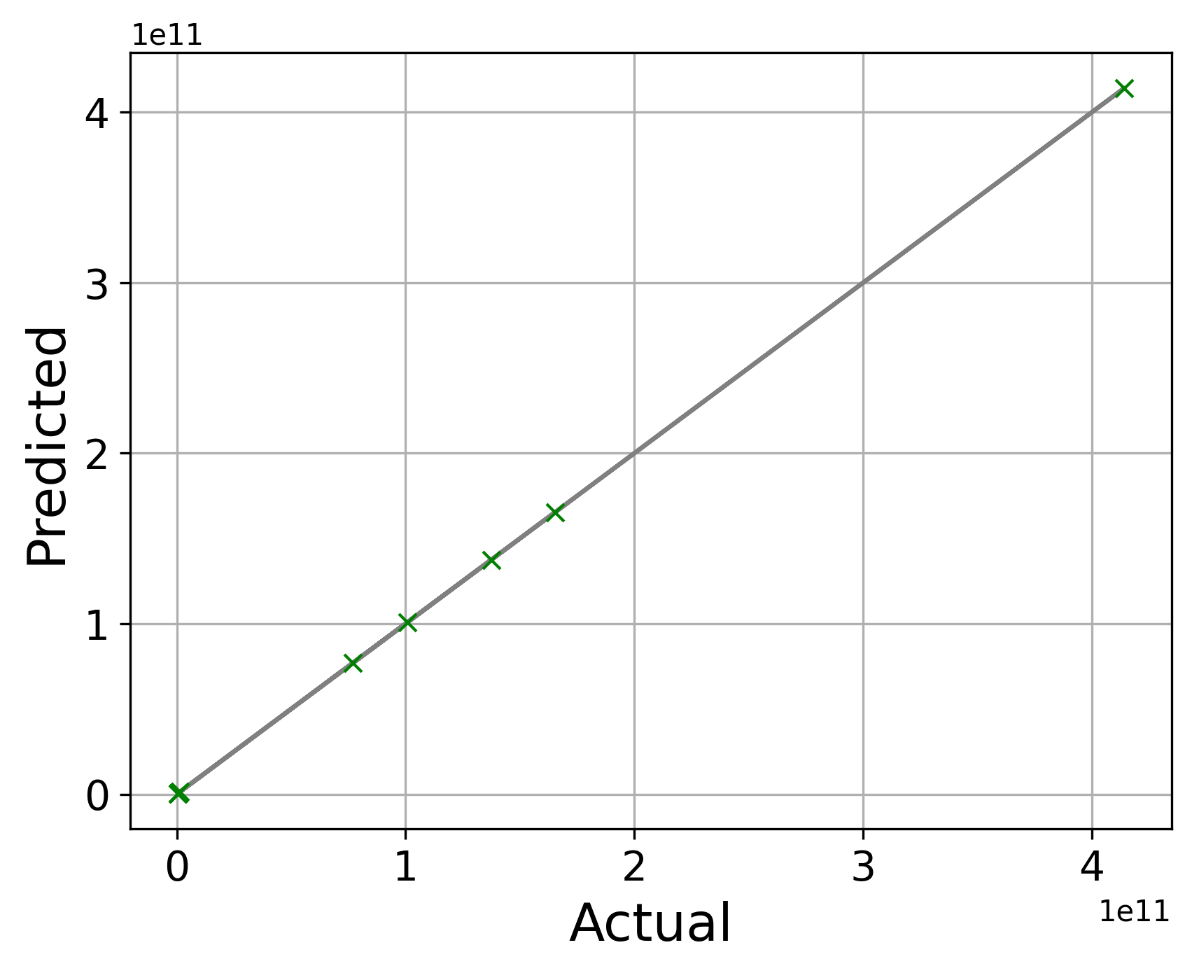
(a) Memory transactions in bytes

(b) Number of load operations

(c) Number of store operations

(d) Number of unconditional branch operations

(e) Number of conditional branch operations

(f) Number of floating point operations

Figure 6: Comparison of different performance metrics between Byfl and static analyzer. Each green ’x’ mark denotes the predicted value, whereas the gray line denotes the actual result from Byfl.

Table 1: List of applications used to validate the static analyzer. LA and DM denote linear algebra and data mining kernels, respectively.

App	Description	Domain
2mm	Two Matrix Multiplications	LA
atax	Matrix Transpose and Vector Multiplication	LA
bicg	BiCG Sub Kernel of BiCGStab Linear Solver	LA
doitgen	Multi-Resolution Analysis kernel	LA
mvt	Matrix Vector Product and Transpose	LA
gemver	Vector Multiplication and Matrix Addition	BLAS
gesummv	Scalar, Vector and Matrix Multiplication	BLAS
gemm	Matrix-Multiply C=alpha.A.B+beta.C	BLAS
symm	Symmetric Matrix-Multiply	BLAS
covariance	Covariance Computation	DM

4 Results

In this section, we validate the results of the static analyzer. First, we validate the programs’ performance metrics using ten applications from different domains from the Polybench [18] benchmark suite. The applications are listed in Table 1. We choose the large dataset of the applications in the Polybench benchmark suite. We compare our results with the results from the Byfl [17]. Byfl is an LLVM-based hardware-independent dynamic instrumentation tool for application characterization, which makes it a suitable choice to validate our results.

Figure 6 shows the comparison of different metrics between the static analyzer and Byfl, where Figures 6(a),  6(b),  6(c),  6(d),  6(e), and 6(f) show the comparison of total memory transactions, load operations, store operations, unconditional branches, conditional branches, and floating point operations respectively for the benchmark kernels. In the figures, the gray line denotes the result from Byfl, where each green ’x’ mark denotes the predicted value from the static analyzer tool. Our results match with Byfl accurately, given that the same LLVM version is used to compile Byfl and in our tool.

Reuse Profile Validation: In this section, we validate our static reuse distance calculation method. To validate, we instrument our target kernel using Byfl [17] and generate a dynamic memory trace. Later, using the parallel tree-based reuse distance calculator, Parda [16], we calculate the dynamic reuse profile of the program. We compare this dynamic reuse distance with the statically calculated reuse profile. Figure 7 shows the reuse profile for the synthetic benchmark in Figure 2, where the X axis represents reuse distance and the Y axis represents the probability of a particular reuse distance P(D). Results show that our approach can calculate reuse profiles correctly with $100\%$ accuracy.

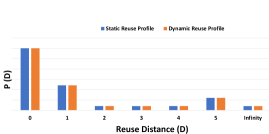
Figure 7: Comparison between statically and dynamically calculated reuse profiles.

5 Limitations

There are several limitations to our approach. First, our reuse calculation approach still needs to be improved in handling pointer/array references. As a result, we still cannot accurately calculate the reuse profiles for the applications listed in Table 1. To support complex cases array references, we must further modify the algorithm 1 to consider complex array reference cases.

Another limitation of our approach is that calculating branch probabilities for data-dependent branch cases can be difficult. For example, each iteration may vary the branch probability for an inner loop’s condition. Although we can calculate overall branch probabilities using arithmetic summation to handle this issue, it should be fully automated. In addition, our static analyzer has yet to support multiple functions.

6 Conclusion

Static analysis can play a vital role in performance modeling and prediction. This paper introduces an architecture-independent LLVM-based static analysis approach to estimate a program’s performance characteristics, including the number of instructions, total memory operations, etc. It also presents a novel static analysis approach to predict the reuse profile of the application kernel, which can be used to predict cache hit rates. The prediction time of our approach is invariant to the input size of the program, which makes our prediction time almost constant and, thus, highly scalable. The results show we can statically predict reuse distance profiles of specific applications quickly and accurately compared to binary instrumentation approaches. Thus, our approach is highly suitable for early-stage design space exploration.

References

- [1] Atanu Barai. Scalable Performance Prediction of Parallel Applications on Multicore Processors Using Analytical Reuse Distance Modeling. PhD thesis, New Mexico State University, December 2022.
- [2] Atanu Barai, Gopinath Chennupati, Nandakishore Santhi, Abdel-Hameed Badawy, Yehia Arafa, and Stephan Eidenbenz. PPT-SASMM: Scalable Analytical Shared Memory Model: Predicting the Performance of Multicore Caches from a Single-Threaded Execution Trace. In The International Symposium on Memory Systems, MEMSYS 2020, page 341–351, New York, NY, USA, 2020. Association for Computing Machinery.
- [3] Antonia Bertolino. Software testing research: Achievements, challenges, dreams. In Future of Software Engineering (FOSE ’07), pages 85–103, 2007.
- [4] Kristof Beyls and Erik H. D’Hollander. Refactoring for data locality. Computer, 42(2):62–71, 2009.
- [5] William R. Bush, Jonathan D. Pincus, and David J. Sielaff. A static analyzer for finding dynamic programming errors. Software: Practice and Experience, 30(7):775–802.
- [6] Calin Cascaval and David A. Padua. Estimating Cache Misses and Locality Using Stack Distances. In Proceedings of the 17th Annual International Conference on Supercomputing, ICS ’03, pages 150–159, New York, NY, USA, 2003. ACM.
- [7] Arun Chauhan and Chun-Yu Shei. Static reuse distances for locality-based optimizations in matlab. In Proceedings of the 24th ACM International Conference on Supercomputing, ICS ’10, page 295–304, New York, NY, USA, 2010. Association for Computing Machinery.
- [8] Gopinath Chennupati, Nandakishore Santhi, Robert Bird, Sunil Thulasidasan, Abdel-Hameed A. Badawy, Satyajayant Misra, and Stephan Eidenbenz. A Scalable Analytical Memory Model for CPU Performance Prediction. In Stephen Jarvis, Steven Wright, and Simon Hammond, editors, High Performance Computing Systems. Performance Modeling, Benchmarking, and Simulation, pages 114–135, Cham, 2018. Springer International Publishing.
- [9] Patrick COUSOT, Radhia COUSOT, Jerome FERET, Antoine MINE, Laurent MAUBORGNE, David MONNIAUX, and Xavier RIVAL. Varieties of static analyzers: A comparison with astree. In First Joint IEEE/IFIP Symposium on Theoretical Aspects of Software Engineering (TASE ’07), pages 3–20, 2007.
- [10] Vijay D’Silva, Daniel Kroening, and Georg Weissenbacher. A survey of automated techniques for formal software verification. IEEE Transactions on Computer-Aided Design of Integrated Circuits and Systems, 27(7):1165–1178, 2008.
- [11] Pär Emanuelsson and Ulf Nilsson. A comparative study of industrial static analysis tools. Electronic Notes in Theoretical Computer Science, 217:5–21, 2008. Proceedings of the 3rd International Workshop on Systems Software Verification (SSV 2008). URL: https://www.sciencedirect.com/science/article/pii/S1571066108003824.
- [12] Chris Lattner and Vikram Adve. LLVM: A Compilation Framework for Lifelong Program Analysis & Transformation. In Proceedings of the International Symposium on Code Generation and Optimization: Feedback-directed and Runtime Optimization, CGO ’04, pages 75–86, Washington, DC, USA, 2004. IEEE Computer Society.
- [13] K.A. Lindlan, J. Cuny, A.D. Malony, S. Shende, B. Mohr, R. Rivenburgh, and C. Rasmussen. A tool framework for static and dynamic analysis of object-oriented software with templates. In SC ’00: Proceedings of the 2000 ACM/IEEE Conference on Supercomputing, pages 49–49, 2000.
- [14] Richard L. Mattson, Jan Gecsei, D. R. Slutz, and I. L. Traiger. Evaluation Techniques for Storage Hierarchies. IBM Syst. J., 9(2):78–117, June 1970.
- [15] Sri Hari Krishna Narayanan and Paul Hovland. Calculating reuse distance from source code. 1 2016. URL: https://www.osti.gov/biblio/1366296.
- [16] Qingpeng Niu, James Dinan, Qingda Lu, and Ponnuswamy Sadayappan. PARDA: A Fast Parallel Reuse Distance Analysis Algorithm. In Proceedings of the 2012 IEEE 26th International Parallel and Distributed Processing Symposium, IPDPS ’12, page 1284–1294, USA, 2012. IEEE Computer Society.
- [17] S. Pakin and P. McCormick. Hardware-independent application characterization. In 2013 IEEE International Symposium on Workload Characterization (IISWC), pages 111–112, Sep. 2013.
- [18] Louis-Noël Pouchet. Polybench: The polyhedral benchmark suite. URL: http://www.cs.ucla.edu/pouchet/software/polybench, 2012.
- [19] Rathijit Sen and David A. Wood. Reuse-based Online Models for Caches. In Proceedings of the ACM SIGMETRICS/International Conference on Measurement and Modeling of Computer Systems, SIGMETRICS ’13, pages 279–292, New York, NY, USA, 2013. ACM.
- [20] Yutao Zhong, Xipeng Shen, and Chen Ding. Program Locality Analysis Using Reuse Distance. ACM Trans. Program. Lang. Syst., 31(6):20:1–20:39, 2009.