Adaptive Bayesian Learning with Action and State-Dependent Signal Variance

Abstract

This manuscript presents an advanced framework for Bayesian learning by incorporating action and state-dependent signal variances into decision-making models. This framework is pivotal in understanding complex data-feedback loops and decision-making processes in various economic systems. Through a series of examples, we demonstrate the versatility of this approach in different contexts, ranging from simple Bayesian updating in stable environments to complex models involving social learning and state-dependent uncertainties. The paper uniquely contributes to the understanding of the nuanced interplay between data, actions, outcomes, and the inherent uncertainty in economic models.

1 Introduction

Bayesian learning, a fundamental concept in statistical inference and decision-making, has gained significant traction across various fields due to its ability to integrate prior knowledge with new information. As a robust methodology, Bayesian learning has been widely acknowledged for its adaptability and precision in handling uncertainty and updating beliefs (Gelman et al.,, 1995).

This manuscript expands upon the Bayesian learning framework (Baley and Veldkamp,, 2023) through uniquely addressing the action and state-dependent signal variance in the agents’ information set. At the core of this framework is the concept that the precision of the signal received by an agent is contingent upon both the agent’s action and the actual state, for example, based on their congruence or tracking error (Daly,, 2018; du Sart and van Vuuren,, 2021; Orlik and Veldkamp,, 2014; Rompotis,, 2011; Stone et al.,, 2013; Yang and Huang,, 2022). For instance, when an action perfectly aligns with the true state, the agent is rewarded with a signal of perfect precision, devoid of any variance. Conversely, any deviation between the action and the true state results in increased signal variance, thus introducing greater uncertainty into the agent’s decision-making process.

This perspective is crucial for a more sophisticated and detailed understanding of decision-making in dynamic environments. Additionally, the adaptive Bayesian learning framework presented in this paper provides an enhanced insight into the data-feedback loop, as conceptualized by Farboodi and Veldkamp, (2021). By accommodating a broader range of sophisticated scenarios within the data economy, this framework elucidates the intricate dynamics of the feedback loop, emphasizing its prevalence and impact in various contexts. This approach not only expands upon traditional Bayesian models but also contributes to a deeper comprehension of the interplay between data, actions, and outcomes in complex economic systems.

We delve into various scenarios within the data-driven economic landscape to showcase how this framework can serve as a unifying approach to understanding the nuanced interplay between actions, states, and signal precision. From simple Bayesian updating in stable environments to intricate models of social learning and state-dependent uncertainties, our exploration reveals the versatility and applicability of this framework across multiple domains.

2 Problem Formalization

2.1 State

The state of the world, denoted as $a^{*}\in{\mathbb{S}}\subset\mathbb{R}$, is an unknown and dynamic element that the agent seeks to estimate. Following a common approach in Bayesian inference due to the distribution’s mathematical properties and its ability to model a wide range of scenarios, the agent’s prior belief about $a^{*}$ is modeled as a normal distribution

$$a^{*}\sim{\mathcal{N}}(\mu_{a},\sigma_{a}^{2}).$$

2.2 Action

The agent chooses an action $a\in{\mathbb{A}}\subset\mathbb{R}$ based on their current belief about the state $a^{*}$. This highlights the decision-making aspect of the agent, where actions are taken based on their understanding and estimation of the state.

2.3 Signal

The signal $s$ observed by the agent is a crucial aspect of the model. It is affected by noise $\epsilon$, which is assumed to be normally distributed with a variance that depends on both the true state and the agent’s action. This dependency from traditional Bayesian learning frameworks is critical, as it introduces a direct link between the agent’s actions and the uncertainty in the information they receive. More formally, the observed signal is given by

$$s=a^{*}+\epsilon,\quad\epsilon\sim{\mathcal{N}}\left(0,\Sigma_{\epsilon}(a^{*},a)\right),$$

with a noise variance function $\Sigma_{\epsilon}:{\mathbb{S}}\times{\mathbb{A}}\to\mathbb{R}$.

2.4 Bayesian Updating

Upon receiving signal $s$, the agent revises their belief about state $a^{*}$. This revision is affected by the action selected, due to the variance of noise that depends on the action. More precisely, the posterior distribution $p(a^{*}|s,a)$, as opposed to merely $p(a^{*}|s)$, is influenced by the selected action $a$, factoring in the action-dependent noise variance. This underscores the dynamic nature of the agent’s belief system, where each new piece of information has the potential to modify their perception of the state.

3 Examples

In this section, we explore different scenarios within the data economy where the concept of action-state-dependent signal precision can be applied as a unifying framework.

Example 1 (Simple Bayesian Updating (Joyce,, 2003)).

Consider a scenario where $\Sigma_{\epsilon}(a^{*},a)\equiv\sigma_{\epsilon}^{2}$ is constant. The posterior distribution then becomes:

$$a^{*}\mid s\sim{\mathcal{N}}\left(\frac{\sigma_{a}^{-2}\mu_{a}+\sigma_{\epsilon}^{-2}s}{\sigma_{a}^{-2}+\sigma_{\epsilon}^{-2}},\frac{1}{\sigma_{a}^{-2}+\sigma_{\epsilon}^{-2}}\right).$$ (1)

This simplistic example illustrates a situation akin to an investor updating their beliefs about the state, such as the future performance of an asset, based on new information. The constant variance $\sigma_{\epsilon}^{2}$ suggests a stable environment, where the uncertainty about future returns does not change with new actions or information. For examples in this simple setting, refer to chapters 2-5 of Veldkamp, (2023).

3.1 Action-Dependent Signal Variance

In the following, we present two examples, in which the uncertainty in the signal varies as the magnitude of the action $a$ varies. A concept here is commonly known as “active learning” or “active experimentation.” For instance, it is exemplified in the bandit problem discussed in Section 3.2 of Veldkamp, (2023), as well as in other examples found in Bergemann and Valimaki, (2006). This approach contrasts with “passive learning.”

Example 2 (Optimal Amount of Data).

The agent decides on $a$, the number of unbiased signals $s_{i}$ to gather, each with iid noises $\epsilon_{i}\sim{\mathcal{N}}(0,\sigma_{\epsilon}^{2})$. They form a sufficient statistic:

$$s=\frac{1}{a}\sum_{i=1}^{n}s_{i}=a^{*}+\frac{1}{a}\sum_{i=1}^{n}\epsilon_{i}\triangleq a^{*}+\epsilon.$$

The noise variance then depends on the number of signals:

$$\Sigma_{\epsilon}(a^{*},a)=\frac{\sigma_{\epsilon}^{2}}{a}.$$

Similar to the posterior update in (1), we have

$$a^{*}\mid s,a\sim{\mathcal{N}}\left(\frac{\sigma_{a}^{-2}\mu_{a}+a\sigma_{\epsilon}^{-2}s}{\sigma_{a}^{-2}+a\sigma_{\epsilon}^{-2}},\frac{1}{\sigma_{a}^{-2}+a\sigma_{\epsilon}^{-2}}\right).$$

This example is analogous to a firm making data-sensitive decisions, such as deciding what data to collect when conducting market research before launching a new product. The more data points (signals) the firm gathers, the lower the uncertainty in noise variance. Despite such a data-collection story, there might be a more sophisticated and heterogeneous underlying mechanism from which the “amount” of data points is determined as shown in the following example.

Example 3 (Social Learning).

In this model, we explore how interactions among agents $i$ lead to varied signal structures. Specifically, the noise variance can be represented as:

$$\Sigma_{\epsilon}(a^{*},a)=\frac{\sigma_{\epsilon}^{2}}{\int_{0}^{1}{\mathbb{I}}_{a_{i}\in{\mathbb{A}}_{i}}di},$$

which reflects the diversity of actions within a potentially endogenous range ${\mathbb{A}}_{i}\subset{\mathbb{A}}$. Moreover, the posterior is

$$a^{*}\mid s,a\sim{\mathcal{N}}\left(\frac{\sigma_{a}^{-2}\mu_{a}+\sigma_{\epsilon}^{-2}s\int_{0}^{1}{\mathbb{I}}_{a_{i}\in{\mathbb{A}}_{i}}di}{\sigma_{a}^{-2}+\sigma_{\epsilon}^{-2}\int_{0}^{1}{\mathbb{I}}_{a_{i}\in{\mathbb{A}}_{i}}di},\frac{1}{\sigma_{a}^{-2}+\sigma_{\epsilon}^{-2}\int_{0}^{1}{\mathbb{I}}_{a_{i}\in{\mathbb{A}}_{i}}di}\right).$$

The above example models the process of agents acquiring information through social learning, a concept derived from the understanding that firms learn from one another about various factors impacting their revenues, such as productivity, market demand, and regulatory changes (Bikhchandani et al.,, 1998). In this context, when an agent $i$ opts for a specific action $a=1$ (from the binary set $\{0,1\}$), like investing in a project, it generates a noisy signal about the project’s return. This signal is then received by other agents, effectively becoming a public signal. The associated noise variance is contingent on the proportion of agents who chose action 1, leading to the expression:

$$\Sigma_{\epsilon}(a^{*},a)=\frac{\sigma_{\epsilon}^{2}}{\int_{0}^{1}{\mathbb{I}}_{a_{i}=1}di}.$$

This formulation is vital for modeling “uncertainty traps” as discussed in works by Fajgelbaum et al., (2017); Saijo, (2017). The posterior mean $\hat{\mu}_{a}=\mathbb{E}[a^{*}\mid s,a]$ and variance $\hat{\sigma}_{a}^{2}=\mathrm{Var}[a^{*}\mid s,a]$ in these scenarios is updated according to the following:

$$\hat{\mu}_{a,t+1}\mid\hat{\mu}_{at},\hat{\sigma}_{at}^{2},a_{t}\sim{\mathcal{N}}\left(\rho\hat{\mu}_{at},\rho^{2}\left(\frac{1}{\hat{\sigma}_{at}^{-2}}-\frac{1}{\hat{\sigma}_{at}^{-2}+\sigma_{\epsilon}^{-2}\int_{0}^{1}{\mathbb{I}}_{a_{it}=1}di}\right)\right),$$

where $\rho<1$ is an AR(1) coefficient in the state evolution of $a_{t}^{*}$.

Most notably, this approach allows for the modeling of data as a by-product of economic activities. During periods of high activity (i.e., when $\int_{0}^{1}\mathbb{I}_{a_{i}=1}di$ is large), more information is disseminated, leading to potentially greater fluctuations in beliefs. The model hence formally explores that agents are hesitant to make decisions due to uncertainty about the environment or the actions of others, which can lead to a lack of economic activities, further generating less data (Kozeniauskas et al.,, 2018) and exacerbating the uncertainty. As we can see, such a feedback loop between data and economic activities also amplifies the business cycle, where booms are times of high activities and information production (Ordonez,, 2013; Van Nieuwerburgh and Veldkamp,, 2006; Veldkamp,, 2005).

3.2 State-Dependent Signal Variance

It should also be noted that the uncertainty might be considered as a hidden state, as suggested by $a^{*}$, in alignment with the perspectives of Ang and Bekaert, (2002) and Orlik and Veldkamp, (2014). In such scenarios, the functional form of noise variance could depend on the actual state, represented by $a^{*}$, as illustrated in the subsequent examples. This is quite realistic in financial markets, where periods of high volatility are often associated with greater unpredictability and more significant discrepancies between the signal and the true state.

Example 4 (Uncertainty Feedback).

Consider a scenario where the state $a^{*}$ represents the volatility of the environment. Define the noise variance as $\Sigma_{\epsilon}(a^{*},a)=f(a^{*})\geq 0$. Under these conditions,

$$s\mid a^{*}\sim{\mathcal{N}}\left(a^{*},f(a^{*})\right),$$

and the posterior distribution is given by

$$p(a^{*}\mid s) \propto p(s\mid a^{*})p(a^{*})$$

$$\propto f(a^{*})^{-\frac{1}{2}}\exp\left(-\frac{(s-a^{*})^{2}}{2f(a^{*})}-\frac{(a^{*}-\mu_{a})^{2}}{2\sigma_{a}^{2}}\right).$$

Figure 1 displays the normalized posterior density for different signal values.

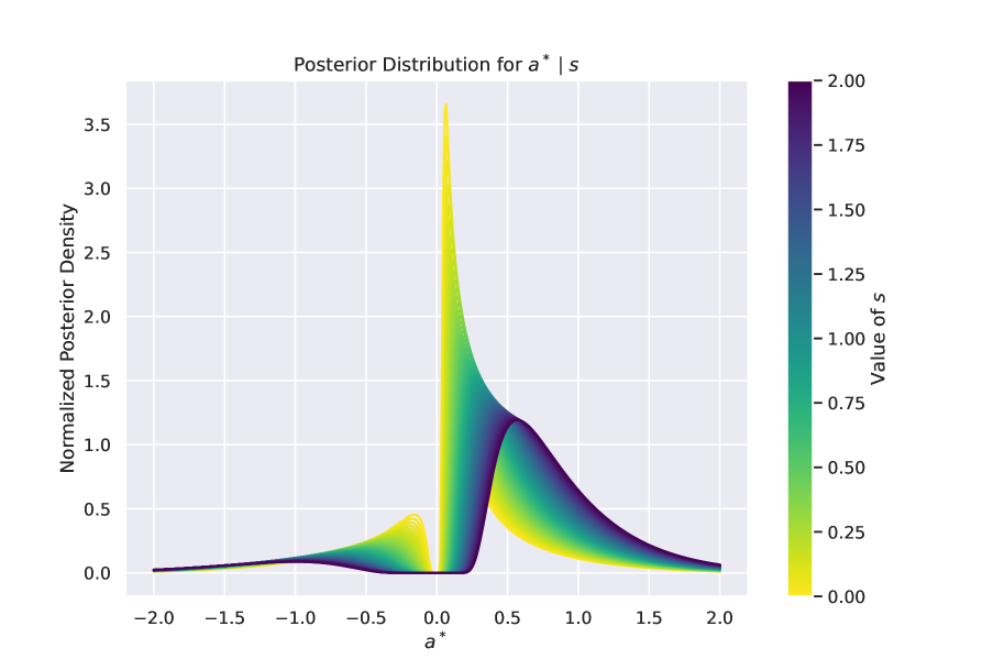
Figure 1: Posterior density of uncertainty feedback, with a standard normal prior, noise variance $f(a^{*})=a^{*2}$, and different signal values.

In this scenario, the noise variance is conceptualized as a function of the actual state of volatility, denoted by $a^{*}$. This formulation models the relationship between volatility and the volatility of volatility. Notably, there is a positive correlation between VVIX and VIX, with several shared peaks, particularly during the financial crisis, as highlighted by Huang et al., (2019). Additionally, the interdependence between the signal variance of volatility and the volatility itself is often influenced by volatility clustering. This phenomenon is characterized by sequences of high (or low) volatility days (Ding and Granger,, 1996; Granger and Ding,, 1995). Furthermore, when stock returns are interpreted as a (potentially biased) signal of volatility, this relationship is exemplified by the leverage effect, which posits an inverse relationship between stock prices and their volatility (Black,, 1976; Christie,, 1982; Schwert,, 1989).

This formulation has also been used in, e.g., Orlik and Veldkamp, (2014). Consider a situation where the state $a^{*}$ takes discrete values, $a^{*}_{1},a^{*}_{2},\ldots,a^{*}_{n}$, each representing a distinct regime or state of the world. The agent has a prior belief about which state the world is in, represented by a discrete probability distribution over these states. Denote the probability of being in state $a^{*}_{i}$ as $p(a^{*}=a^{*}_{i})$.

Example 5 (Discrete Regimes).

The noise variance in this scenario is a function of the state, $\Sigma_{\epsilon}(a^{*},a)=f(a^{*})\geq 0$, where $f$ is a function mapping states to their respective noise variances. This variance could represent the level of uncertainty or instability associated with each state. The observed signal $s$ is still given by

$$s\mid a^{*}\sim{\mathcal{N}}\left(a^{*},f(a^{*})\right).$$

Upon observing $s$, the agent updates their belief about the current state $a^{*}$ according to Bayes’ theorem:

$$p(a^{*}=a^{*}_{i}\mid s)=\frac{p(s\mid a^{*}=a^{*}_{i})p(a^{*}=a^{*}_{i})}{\sum_{j=1}^{n}p(s\mid a^{*}=a^{*}_{j})p(a^{*}=a^{*}_{j})}.$$

Furthermore, in a regime-switching model (Ang and Bekaert,, 2002; Bekaert et al.,, 2001; Hamilton,, 1989), if $a^{*}$ evolves according to a Markov process, the transition probabilities between states can be used to update the prior probabilities $p(a^{*}=a^{*}_{i})$ for the next time period, based on the current posterior probabilities. This model can be particularly useful in scenarios where different regimes or states have distinct characteristics and levels of uncertainty, such as in financial markets where different market conditions (e.g., bull market, bear market, or high volatility period) can significantly affect investment decisions and risk assessments.

3.3 Action-State-Dependent Signal Variance

Example 6 (Tracking Error).

The signal noise variance can be related to the discrepancy between the action $a$ and the true state $a^{*}$:

$$\Sigma_{\epsilon}(a^{*},a)=k|a-a^{*}|^{2}$$

for some constant $k>0$.

This model could represent a bandit problem, in which a firm implements a project $a_{j}$ and observes a project-specific output as a signal

$$s_{j}=A-(a_{j}-a_{j}^{*})^{2}.$$

The signal structure implies a constant output $A$ delivered by the implementation, minus a penalty for not being close to an unobserved project-specific target $a_{j}^{*}$.

Remarkably, Example 6 extends to dynamic settings, linking forecast error to economic uncertainty (Orlik and Veldkamp,, 2014). Here, agent $i$ forecasts the future state at $t+1$ using current information ${\mathcal{I}}_{it}(a_{it})$ dependent on their action $a_{it}$. The ex-post forecast error at time $t$ is:

$$\epsilon_{i,t+1}=\left|a_{t+1}^{*}-\mathbb{E}[a_{t+1}^{*}\mid{\mathcal{I}}_{it}(a_{it})]\right|.$$

In scenarios like predicting GDP growth, the environment’s uncertainty is indicated by the expected forecast error. This could also lead to noisier public signals through the variance term:

$$\Sigma_{\epsilon}(a_{t}^{*},a_{t})=\int_{0}^{1}\mathbb{E}[\epsilon_{i,t+1}^{2}\mid{\mathcal{I}}_{it}(a_{it})]di.$$

4 Conclusions

Overall, this manuscript provides a comprehensive and nuanced understanding of Bayesian learning in dynamic environments, emphasizing the interplay between actions, states, and signal precision. The variety of examples presented showcases the framework’s applicability across different scenarios, from stable environments to more complex situations involving heterogenous cross-sectional interactions and richer longitudinal structures.

References

- Ang and Bekaert, (2002) Ang, A. and Bekaert, G. (2002). Regime switches in interest rates. Journal of Business & Economic Statistics, 20(2):163–182.
- Baley and Veldkamp, (2023) Baley, I. and Veldkamp, L. (2023). Bayesian learning. In Handbook of Economic Expectations, pages 717–748. Elsevier.
- Bekaert et al., (2001) Bekaert, G., Hodrick, R. J., and Marshall, D. A. (2001). Peso problem explanations for term structure anomalies. Journal of Monetary Economics, 48(2):241–270.
- Bergemann and Valimaki, (2006) Bergemann, D. and Valimaki, J. (2006). Bandit problems.
- Bikhchandani et al., (1998) Bikhchandani, S., Hirshleifer, D., and Welch, I. (1998). Learning from the behavior of others: Conformity, fads, and informational cascades. Journal of economic perspectives, 12(3):151–170.
- Black, (1976) Black, F. (1976). Studies of stock market volatility changes. Proceedings of the American Statistical Association, Business & Economic Statistics Section, 1976.
- Christie, (1982) Christie, A. A. (1982). The stochastic behavior of common stock variances: Value, leverage and interest rate effects. Journal of financial Economics, 10(4):407–432.
- Daly, (2018) Daly, M. (2018). Feasible portfolios under tracking error, , and utility constraints. Investment Management & Financial Innovations, 15(1):141.
- Ding and Granger, (1996) Ding, Z. and Granger, C. W. (1996). Modeling volatility persistence of speculative returns: a new approach. Journal of econometrics, 73(1):185–215.
- du Sart and van Vuuren, (2021) du Sart, C. F. and van Vuuren, G. W. (2021). Comparing the performance and composition of tracking error constrained and unconstrained portfolios. The Quarterly Review of Economics and Finance, 81:276–287.
- Fajgelbaum et al., (2017) Fajgelbaum, P. D., Schaal, E., and Taschereau-Dumouchel, M. (2017). Uncertainty traps. The Quarterly Journal of Economics, 132(4):1641–1692.
- Farboodi and Veldkamp, (2021) Farboodi, M. and Veldkamp, L. (2021). A model of the data economy. Technical report, National Bureau of Economic Research.
- Gelman et al., (1995) Gelman, A., Carlin, J. B., Stern, H. S., and Rubin, D. B. (1995). Bayesian data analysis. Chapman and Hall/CRC.
- Granger and Ding, (1995) Granger, C. W. and Ding, Z. (1995). Some properties of absolute return: An alternative measure of risk. Annales d’Economie et de Statistique, pages 67–91.
- Hamilton, (1989) Hamilton, J. D. (1989). A new approach to the economic analysis of nonstationary time series and the business cycle. Econometrica: Journal of the econometric society, pages 357–384.
- Huang et al., (2019) Huang, D., Schlag, C., Shaliastovich, I., and Thimme, J. (2019). Volatility-of-volatility risk. Journal of Financial and Quantitative Analysis, 54(6):2423–2452.
- Joyce, (2003) Joyce, J. (2003). Bayes’ theorem.
- Kozeniauskas et al., (2018) Kozeniauskas, N., Orlik, A., and Veldkamp, L. (2018). What are uncertainty shocks? Journal of Monetary Economics, 100:1–15.
- Ordonez, (2013) Ordonez, G. (2013). The asymmetric effects of financial frictions. Journal of Political Economy, 121(5):844–895.
- Orlik and Veldkamp, (2014) Orlik, A. and Veldkamp, L. (2014). Understanding uncertainty shocks and the role of black swans. Technical report, National bureau of economic research.
- Rompotis, (2011) Rompotis, G. G. (2011). Predictable patterns in etfs’ return and tracking error. Studies in Economics and Finance, 28(1):14–35.
- Saijo, (2017) Saijo, H. (2017). The uncertainty multiplier and business cycles. Journal of Economic Dynamics and Control, 78:1–25.
- Schwert, (1989) Schwert, G. W. (1989). Why does stock market volatility change over time? The journal of finance, 44(5):1115–1153.
- Stone et al., (2013) Stone, L. D., Streit, R. L., Corwin, T. L., and Bell, K. L. (2013). Bayesian multiple target tracking. Artech House.
- Van Nieuwerburgh and Veldkamp, (2006) Van Nieuwerburgh, S. and Veldkamp, L. (2006). Learning asymmetries in real business cycles. Journal of monetary Economics, 53(4):753–772.
- Veldkamp, (2005) Veldkamp, L. L. (2005). Slow boom, sudden crash. Journal of Economic theory, 124(2):230–257.
- Veldkamp, (2023) Veldkamp, L. L. (2023). Information choice in macroeconomics and finance. Princeton University Press.
- Yang and Huang, (2022) Yang, T. and Huang, X. (2022). Active or passive portfolio: A tracking error analysis under uncertainty theory. International Review of Economics & Finance, 80:309–326.