Amplitude-Ensemble
Quantum-Inspired Tabu Search Algorithm
for Solving 0/1 Knapsack Problems

Abstract

In this paper, we introduce an enhanced version of the “Quantum-inspired Tabu Search Algorithm” (QTS), termed “amplitude-ensemble” QTS (AE-QTS). By utilizing population information, we bring QTS closer to the quantum algorithm – Glover Search Algorithm, maintaining algorithmic simplicity. AE-QTS is validated against the 0/1 knapsack problem, showing at least a 20% performance boost across all problems and over a 30% efficiency increase in some cases compared to the original QTS. Even with increasingly complex problems, this method consistently outperforms the original QTS.

I Introduction

Metaheuristic has always been a hot research field because such methods can be used to solve highly complex problems, including NP-complete and NP-hard problems. Consequently, many researchers have devoted considerable effort to this field, resulting in the invention of outstanding and efficient metaheuristic algorithms like Simulated Annealing (SA) [1], Genetic Algorithm (GA) [2], Particle Swarm Optimization (PSO) [3], Ant Colony Optimization (ACO) [4], Artificial Bee Colony (ABC) [5], Differential Evolution (DE) [6], Tabu Search (TS) [7, 8], and others.

At the same time, Quantum Algorithms [9, 10, 11] are also making remarkable achievements. The algorithms executed by quantum computers have even shaken the entire cryptographic world. This success has encouraged researchers to integrate quantum characteristics into the design of metaheuristic algorithms, giving birth to many excellent quantum-inspired algorithms such as Quantum-inspired Evolutionary Algorithm (QEA) [12], Quantum-inspired Genetic Algorithm (QGA) [13], Quantum-inspired Ant Colony Optimization (QACO) [14], Quantum-inspired Particle Swarm Optimization (QPSO) [14], Quantum-inspired Differential Evolution (QDE) [15, 16], Quantum-inspired Tabu Search (QTS) [17, 18], and others. All these algorithms have greatly benefited from the enhancement of search performance by the concept of quantum characteristics.

However, only two algorithms, QEA [12] and QTS [17, 18], are mainly conceived from the perspective of quantum characteristics. QEA [12] still leans slightly towards the traditional population-based thinking but perfectly mirrors the concept of improving observation probability in quantum algorithms [9, 10, 11] through quantum bit measurement and quantum state updating. This characteristic utilization is further maximized in the QTS algorithm [17, 18]. QTS [17, 18] perfectly mirrors the entire concept of the Glover Search Algorithm [11] by comparing each bit to identify the trend of each bit through finding the best and worst solutions in each iteration of the population. It then uses this trend and a rotation matrix to adjust the state of the quantum bit at this position, closely resembling the probability adjustment of a solution in each iteration in the Glover Search Algorithm [11].

The quantum-inspired algorithms derived closer to pure quantum algorithms [9, 10, 11] are structurally simpler and have no ambiguous space, unlike other metaheuristic methods where many components have various implementations, making them difficult to replicate experiments or apply to other problems. Among quantum-inspired algorithms, QTS [17, 18] is the simplest and easiest to replicate. All components in its algorithm have well-defined implementation methods, leaving no ambiguous space. Experimental results have shown that QTS [17, 18] is not only simple to implement and fast in operation but also more effective than QEA [12], finding the optimal solution more quickly and stably.

Although the idea of QTS [17, 18] is already superior, its performance has not yet been maximized. The solutions generated by each iteration of the population only screen out two sets of solutions to update the quantum state. Obviously, other sets of solutions are wasted, but these solutions are also generated by quantum bits containing all the information. This information should also return to all quantum bits, just like the Glover Search Algorithm [11]. If you want to adjust the amplitude of a particular solution, you must take into account the amplitude of all other sets of solutions. Therefore, how to reintegrate the information of the remaining population into the quantum bits becomes extremely important.

II Controbutions

This section elaborates in detail the contributions of this study. In fact, the QTS algorithm [17, 18] is already highly efficient and simplistic, making it quite challenging to enhance the essence of the algorithm further. At most, improvements can be made by adding external components when implementing it for different problems to cater to their specific needs. Remarkably, our study manages to enhance the very nature of the QTS algorithm [17, 18] and achieves exceptional efficiency, a feat that is not easily accomplished. The contributions of our research are summarized as follows:

1. We’ve enhanced QTS [17, 18] on the foundation of its original algorithm design, attaining at least an approximate 20% boost in performance, with some problems exhibiting over a 30% improvement. When confronted with more intricate challenges, the quality of the solutions found also exceeds that of the original QTS [17, 18]. Additionally, this advancement is compatible with issues previously addressed using QTS [17, 18]; only the section concerning the quantum state update requires modification.

2. Our algorithm maintains the simplicity and ease of implementation inherent to QTS [17, 18]. Unlike other traditional metaheuristics, QTS [17, 18] boasts a straightforward implementation, attributed to its unambiguous internal components. Each element within the algorithm is free of ambiguity, preventing varied interpretations and coding approaches. Consequently, it doesn’t spawn different adaptations or extensions, ensuring a rapid and straightforward implementation that exhibits consistent search capability across diverse problems.

3. The proposed algorithm retains the original number of parameters in QTS [17, 18]. Often, many improvement strategies introduce additional parameters requiring adjustment. However, our enhancement method doesn’t add any parameters, eliminating the need for retesting or adjusting other variables.

III Quantum Computing Principles

The fundamental unit of a quantum computer is the quantum bit, abbreviated as qubit. Qubits exist in wave-like forms, so each state has its corresponding amplitude. Consequently, all states have their observed probabilities. When a qubit is in a particular state and used for computation, it can carry an infinite amount of information. This characteristic allows for achieving parallel computation. However, the most challenging part is not designing computational methods but rather designing the adjustment of amplitudes to increase the probability of observing the target state. The current two quantum-inspired algorithms are both designed based on this concept. Next, we will introduce quantum bits and their corresponding gates.

III-A Quantum bit

A quantum bit is abbreviated as a qubit. It encompasses two states, represented as $\ket{0}$=$\begin{pmatrix}1\\ 0\end{pmatrix}$ and $\ket{1}$=$\begin{pmatrix}0\\ 1\end{pmatrix}$, which can also be viewed as the $\hat{x}$ and $\hat{y}$ axes in a two-dimensional plane. Unlike classical bits that are in either the 0 or 1 state, a quantum bit can exist in a superposition of both $\ket{0}$ and $\ket{1}$ states at the same time, referred to as a superposition state. The superposition state can be seen as a point on the circle in the two-dimensional plane, as shown in Fig. 1. Therefore, it can be expressed as: $\ket{\phi}=\alpha\ket{0}+\beta\ket{1}$, where $\left|\alpha\right|^{2}$ represents the probability of obtaining $\ket{0}$ when measuring this qubit, $\left|\beta\right|^{2}$ represents the probability of obtaining $\ket{1}$ when measuring this qubit, and $\left|\alpha\right|^{2}+\left|\beta\right|^{2}=1$.

III-B Quantum gate

The distinction between quantum logic gates and conventional computer logic gates lies in the reversibility of the former, as they all perform unitary operations, denoted as $UU^{*}=U^{*}U=I$. There are numerous types of quantum logic gates; however, this study exclusively utilizes rotation matrices.

$$\binom{\alpha^{{}^{\prime}}}{\beta^{{}^{\prime}}}=\begin{pmatrix}\cos(\bigtriangleup\theta)&-\sin(\bigtriangleup\theta)\\ \sin(\bigtriangleup\theta)&\cos(\bigtriangleup\theta)\end{pmatrix}\binom{\alpha}{\beta}$$ (1)

Referring to the Fig. 1, $\alpha^{{}^{\prime}}$ and $\beta^{{}^{\prime}}$ represent the coordinates post-rotation, and the probabilities of obtaining $\ket{0}$ and $\ket{1}$ upon measurement of the quantum bit can be modified through the rotation matrix. It is essential to note that the operation involves clockwise rotation. Consequently, in the second and fourth quadrants, rotation is executed using $-\bigtriangleup\theta$.

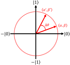
Figure 1: Polar plot of the rotation matrix on a qubit.

IV 0/1 knapsack problem

The 0/1 knapsack problem is a classic combinatorial optimization problem. Generally, there are $K$ items to choose from, each of which can either be taken or left behind. Each item has a specific value and weight. The knapsack also has a weight limit $C$, making it impossible to take all items. The goal of this problem is to maximize the total value of the items taken, while adhering to the weight constraint of the knapsack. Here, we define the knapsack problem as adopted in this study: $p_{i}=$ profit of item $i$, $w_{i}=$ weight of item $i$, $c_{i}=$ capacity of knapsack $i$, and $C=\frac{1}{2}\sum_{i=1}^{K}w_{i}$.
The objective of this problem is to maximize

$$f(x)=\sum_{i=1}^{K}p_{i}x_{i},$$

subject to the constraint

$$\sum_{i=1}^{K}w_{i}x_{i}\leq C.$$

Here, $x=\left(x_{1},x_{2},...,x_{k}\right)$, with $x_{i}$ being 0 or 1, $p_{i}$ representing the value of the $i$th item, and $w_{i}$ denoting the weight of the $i$th item. $C$ is the maximum capacity of the knapsack. If $x_{i}=1$, it indicates that the $i$th item has been selected to be placed in the knapsack.

This problem can be simply categorized into three cases, each with different methods of generating weights and values, as follows: 1.4cm

The weight $w_{i}$ is uniformly random selected from the range $\left[1,10\right]$, and the value $p_{i}$ is calculated as $w_{i}+5$.

The weight $w_{i}$ is uniformly random selected from the range $\left[1,10\right]$, and the value $p_{i}$ is calculated as $w_{i}+l_{i}$, where $l_{i}$ is uniformly random selected from the range $\left[0,5\right]$.

The weight $w_{i}$ is within the range $\left\{x\in\mathbb{Z}:1\leq x\leq 10\right\}$. The values of $w_{i}$ are generated sequentially and in a cyclic manner, for example, $w=\left(1,2,...,10,1,2,...\right)$. The value $p_{i}$ is calculated as $w_{i}+5$.

V amplitude-ensemble QTS (AE-QTS)

This method is derived from QTS [17, 18], where QTS selects the best and worst from each iteration to determine the rotation of each quantum bit. It’s a highly effective strategy, and experiments have confirmed its capability to precisely adjust the amplitude of quantum bits. In this study, we adopt this method but expand its scope to encompass the entire population of each iteration. Doing so enables a more efficient incorporation of all explored information into the quantum bits.

Thus, the only difference between this study and QTS [17, 18] lies in the approach at line 9 of Algo. 1; all other steps are the same. Below is a detailed explanation of each step.

1. Set the iteration $t$ to be 0.

2. $Q(0)=\left(\begin{array}[]{c|c|c|c}\begin{matrix}\alpha_{1}\\ \beta_{1}\end{matrix}&\begin{matrix}\alpha_{2}\\ \beta_{2}\end{matrix}&\begin{matrix}...\\ ...\end{matrix}&\begin{matrix}\alpha_{k}\\ \beta_{k}\end{matrix}\end{array}\right)$, where $k$ is the number of qubits, equivalent to the number of items with the knapsack problem. During the initialization phase, all values of $\alpha$ and $\beta$ are set to $\frac{1}{\sqrt{2}}$. This implies that when measuring these quantum bits, there is an equal probability of measuring $\ket{0}$ or $\ket{1}$.

3. The best solution $s^{b}$ is selected from $P(t)$, which was measured from $Q(t)$, repaired, and evaluated again within $P(t)$.

4. The portion from the $4th$ line to the $14th$ line constitutes the core of this method, which will be executed repeatedly until reaching the maximum number of iterations.

5. make $P(t)$ implies generating $N$ sets of solutions by measuring $Q(t-1)$ for $N$ times, where these solutions are represented in binary encoding, signifying the selection or non-selection of items. For example, if $N=2$, $K=3$, and $Q(t-1)=\left(\begin{array}[]{c|c|c}\begin{matrix}\alpha_{1}\\ \beta_{1}\end{matrix}&\begin{matrix}\alpha_{2}\\ \beta_{2}\end{matrix}&\begin{matrix}\alpha_{3}\\ \beta_{3}\end{matrix}\end{array}\right)$. In this case, 6 measurements are needed to generate 2 sets of binary solutions with a length of 3. The probabilities of obtaining ‘0’ and ‘1’ are $\left|\alpha_{k}\right|^{2}$ and $\left|\beta_{k}\right|^{2}$, where $k=1,2,3$, respectively, as shown below: $\begin{pmatrix}1&0&0\\ 1&1&0\end{pmatrix}$.

6. repair $P(t)$ means that when the total weight exceeds the capacity of the backpack, it is necessary to perform repairs by removing some items to reduce the weight. However, if the total weight is less than the knapsack’s capacity, attempts can be made to add some items back, while trying to maximize the knapsack’s carrying capacity during the repair process as much as possible.

7. evaluate $P(t)$ means assessing the profits obtained for each set of selections. There are a total of $N$ feasible solutions here, so it will return the profits corresponding to the $N$ feasible solutions.

8. update $Q(t-1)$ means updating the state of quantum bits. This is the only difference from QTS. In QTS, the contemporary best and worst solutions are taken from $P(t)$, and a comparison is made using the corresponding bits. The rotation angles for each bit are determined according to Table I for the rotation matrix operation. In this study, the population is sorted based on profit. Then, pairs are selected as follows: the best and worst, the second best and second worst, the third best and third worst, and so on, up to $N/2$ pairs (shown in Fig. 2). The first pair is operated on with $\Delta\theta/1$ for the rotation matrix, the second pair with $\Delta\theta/2$, the third pair with $\Delta\theta/3$, and so on, following this pattern. Quantum state adjustments are made using these pairs according to Table I. In total, $N/2$ rotation matrix operations are performed.

9. The next step is to evaluate whether the best solution found in this iteration of the population is better than the currently recorded best solution. If it is, a replacement is made. Consequently, this measure ensures that $s^{b}$ always represents the best binary solution found throughout the algorithm’s execution.

Algorithm 1 Amplitude-Ensemble QTS

1:$t\leftarrow 0$

2:initialize $Q(t)$

3:initialize the best solution $s^{b}$ from $P(t)$ by measuring $Q(t)$, repairing and evaluating $P(t)$

4:while $t<$ MAX_GEN do

5:     $t\leftarrow t+1$

6:     make $P(t)$ with $N$ solutions by measuring $Q(t-1)$

7:     repair $P(t)$

8:     evaluate $P(t)$

9:     update $Q(t)$ by $P(t)$ $\triangleright$ The difference from QTS

10:     select the best solution $b$ from $P(t)$

11:     if $b>s^{b}$ then

12:         $s^{b}\leftarrow b$

13:     end if

14:end while

Algorithm 2 Repair($s$)

1:$s=\left(x_{1},x_{2},...,x_{k}\right)$

2:knapsack-overfilled $\leftarrow$ false

3:if $\sum_{i=1}^{K}w_{i}x_{i}>C$ then

4:     while knapsack-overfilled do

5:         random select $j$th item from $s$

6:         $s_{j}\leftarrow 0$

7:         if $\sum_{i=1}^{K}w_{i}x_{i}\leq C$ then

8:              knapsack-overfilled $\leftarrow$ false

9:         end if

10:     end while

11:     while not knapsack-overfilled do

12:         random select $j$th item from $s$

13:         $s_{j}\leftarrow 1$

14:         if $\sum_{i=1}^{K}w_{i}x_{i}>C$ then

15:              knapsack-overfilled $\leftarrow$ true

16:         end if

17:     end while

18:end if

Algorithm 3 Update($n$)

1:$i\leftarrow 0$

2:$index\leftarrow$ sort $P(t)$ with profits by DESC

3:while $i<N/2$ do

4:     $best\leftarrow index[i]$

5:     $worst\leftarrow index[N-1-i]$

6:     $j\leftarrow 0$

7:     while $j<K$ do

8:         $t\leftarrow i+1$

9:         Determine $\Delta\theta$ by $best_{j}$ and $worst_{j}$ in Table I

10:         $q_{j}=\begin{pmatrix}cos(\Delta\theta/t)&-sin(\Delta\theta/t)\\ sin(\Delta\theta/t)&cos(\Delta\theta/t)\end{pmatrix}\begin{pmatrix}\alpha_{j}\\ \beta_{j}\end{pmatrix}$

11:         $j\leftarrow j+1$

12:     end while

13:     $i\leftarrow i+1$

14:end while

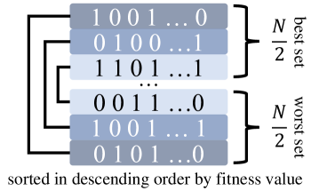
Figure 2: The selection pair in $P(t)$.

TABLE I: Rotation lookup table

$s^{b}_{i}$	$s^{w}_{i}$	$Q_{i}\in T$	$\Delta\theta$
$Q_{i}$ locates in first or third quadrant
0	0	True	0
0	1	False	$-\theta$
1	0	False	$+\theta$
1	1	True	0
$Q_{i}$ locates in second or fourth quadrant
0	0	True	0
0	1	False	$+\theta$
1	0	False	$-\theta$
1	1	True	0
$i=1,2,...,k,$ where $k$ is the number of qubit

VI Experiments

Here, we will use the abbreviation AE-QTS to refer to our method for the sake of simplicity in discussing the experimental result figures later on. For the experiments, we wrote the program using Python and initially compared it with QTS [17, 18] to validate the characteristic of enhanced performance by integrating population information into QTS [17, 18]. Once this characteristic is confirmed, it should consistently exist regardless of variations in the problems or when facing different issues. In this context, we conducted validations using three cases.

We will proceed with experiments involving 100 items, 250 items, and 500 items respectively. Both algorithms will have identical parameters, with population size $N=10$, $\Delta\theta=0.01\pi$, and $MAX\_GEN=1000$. The experimental results are illustrated in Fig. 3, Fig. 4, and Fig. 5. In all three different scenarios, regardless of how the experimental conditions are varied, the convergence speed of our method consistently outperforms QTS [17, 18]. Moreover, the quality of the solutions obtained is comparable to those achieved by the QTS algorithm [17, 18], and in some cases, our method even excels beyond QTS.

However, in all experiments involving 500 items across various cases, it appeared that QTS [17, 18] was still converging towards the end. Consequently, we extended the number of iterations to 2000 in an attempt to allow QTS [17, 18] to fully converge before comparing the quality of solutions obtained by both methods. The results are shown in Fig. 6 and Fig. 7. When QTS [17, 18] fully converges, at most, it equates to AE-QTS, indicating that AE-QTS had already converged to the optimal solution much earlier. Furthermore, in more complex problems, the quality of the final solution attained by AE-QTS is superior to that of QTS [17, 18], as illustrated in Fig. 7, proving the comprehensive superiority of AE-QTS in optimization capability.

Lastly, we added a variable in all the experiments to record the iteration of the last update to the global optimal. By averaging the final values of the iteration, we derived the overall improvement in performance, as primarily shown in Table II. Consequently, the “amplitude-ensemble” mechanism demonstrates an approximate performance increase of 34%, 27%, and 20% for problems with 100, 250, and 500 items, respectively, when comparing with the QTS algorithm. Although this performance improvement might diminish as the problem’s complexity increases, it still consistently maintains a boost of nearly 20%. By examining the various experimental results, it is evident that the AE-QTS consistently outperforms QTS during the convergence process. The advantage of this method becomes more pronounced in complex problems, underscoring the superiority of our approach.

TABLE II: The performance improvement comparison

CASE #	Num. of item	QTS1	AE-QTS1	PoI
I	100	381.86	230.77	39.57%
	250	720.02	590.76	17.95%
	500	905.14	765.02	15.48%
II	100	359.72	257.45	28.43%
	250	785.76	539.08	31.39%
	500	951.29	815	14.33%
III	100	209.24	140.73	32.74%
	250	454	304.26	32.98%
	500	716.78	503.27	29.79%
The average improvement ratios: 33.58% (100 items), 27.44% (250 items), 19.86% (500 items)
Note1: The average iteration for the last update of the global optimal.
PoI: Percentage of improvement

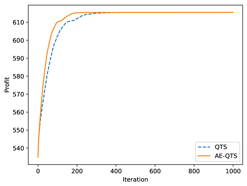
(a) 100 items

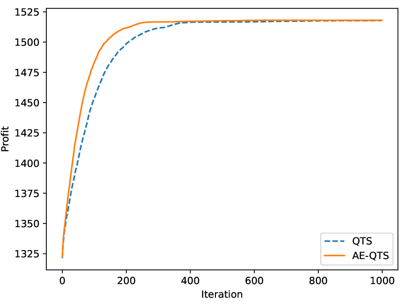
(b) 250 items

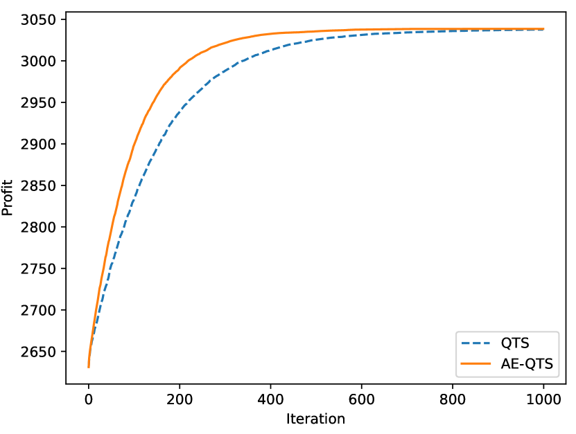
(c) 500 items

Figure 3: Case I: 100, 250, and 500 items.

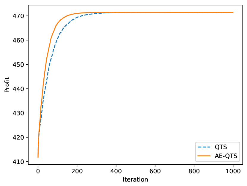
(a) 100 items

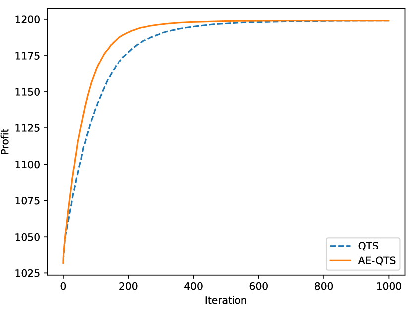
(b) 250 items

(c) 500 items

Figure 4: Case II: 100, 250, and 500 items.

(a) 100 items

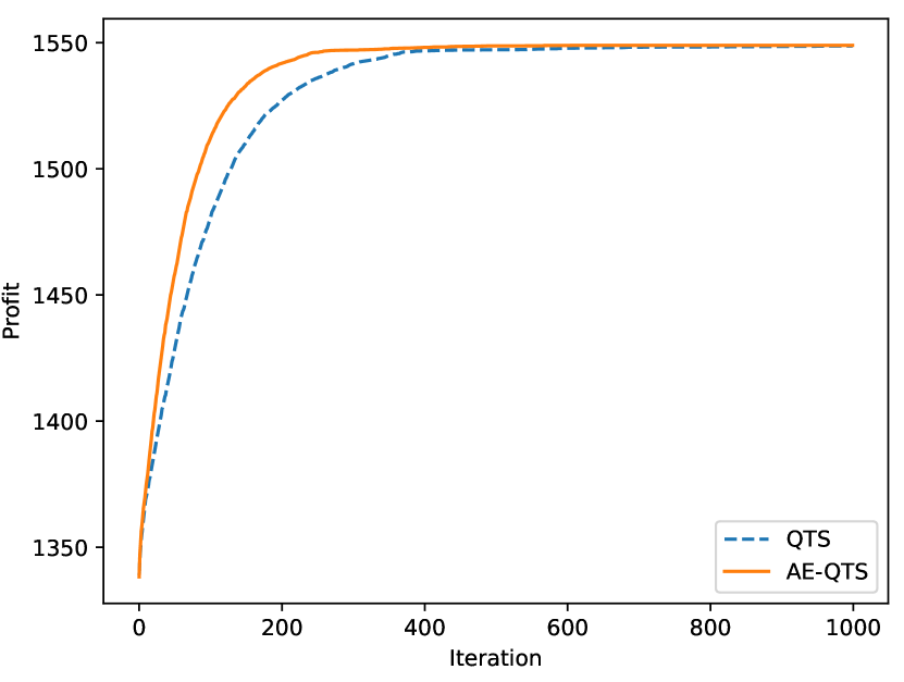
(b) 250 items

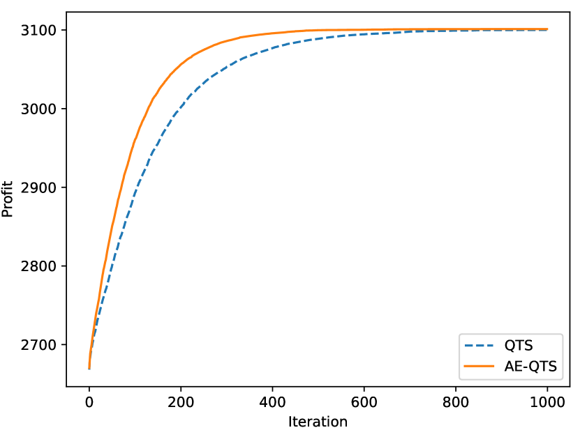
(c) 500 items

Figure 5: Case III: 100, 250, and 500 items.

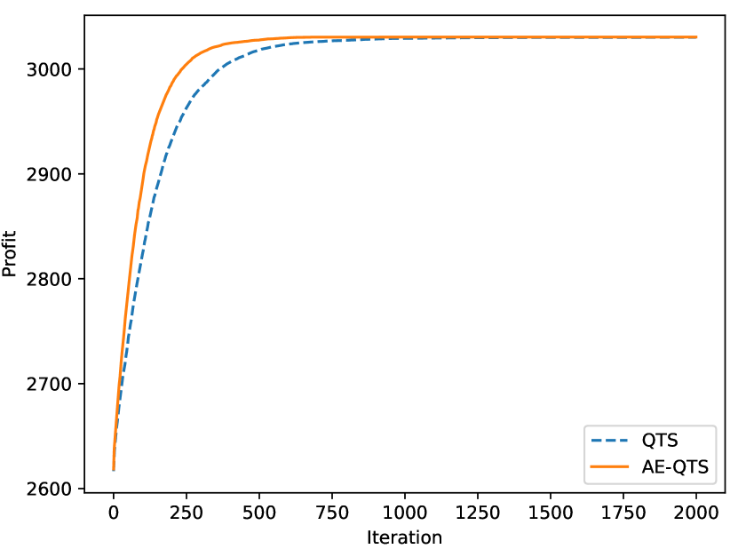
(a) Case I

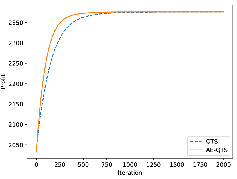
(b) Case II

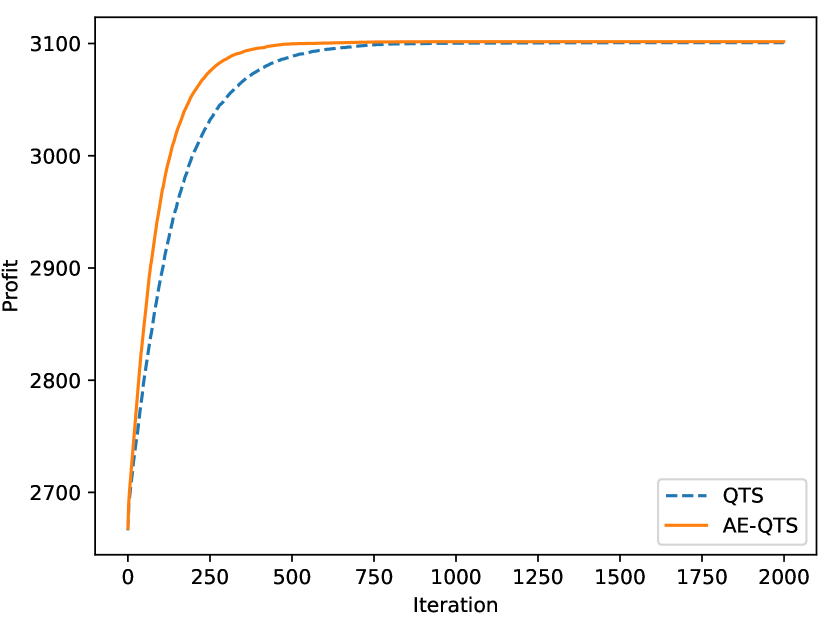
(c) Case III

Figure 6: Three cases with 500 items and 2000 iterations.

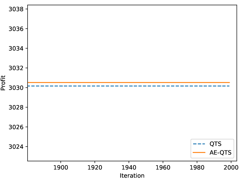
(a) Case I

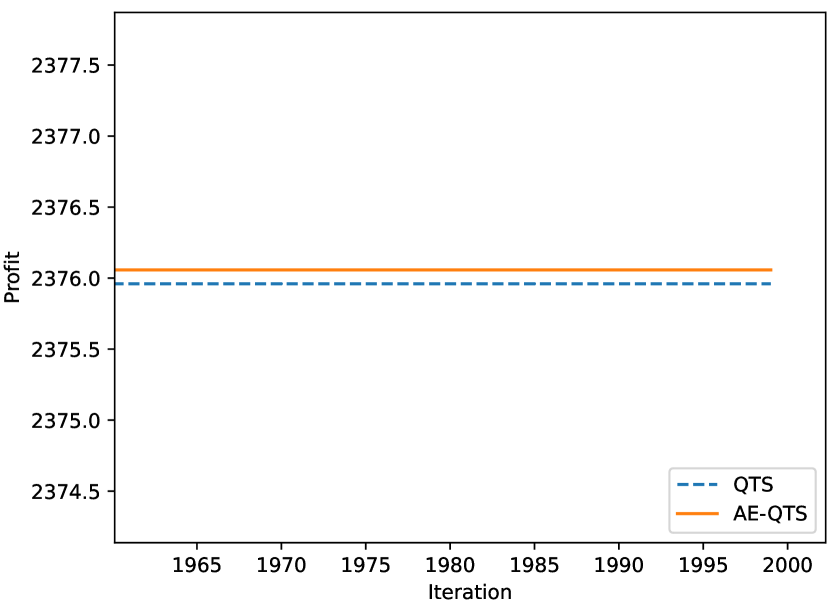
(b) Case II

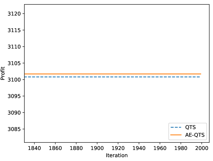
(c) Case III

Figure 7: Three cases with 500 items and 2000 iterations at maximum zoom.

VII Conclusion

In this study, we successfully incorporated the population concept of Glover Search Algorithm [11] into all the quantum bits of AE-QTS, achieving at least approximately a 20% increase in the efficiency of QTS [17, 18]. In complex problems, the quality of the solutions found by AE-QTS also manages to exceed that of QTS [17, 18]. Given that QTS’s inherent performance already surpasses that of typical metaheuristic methods, this increment in efficiency is indeed a remarkable contribution.

Furthermore, the enhancement technique introduced in this study does not increase the inherent complexity of QTS [17, 18], nor does it alter the core structure of QTS [17, 18]. This allows for straightforward modifications to be made to existing methods that utilize QTS [17, 18], facilitating this performance boost. It implies that every approach that centers around QTS [17, 18] can benefit from this augmentation in efficiency.

In conclusion, our study maintains the simplicity of the QTS method [17, 18], adding no additional parameters. The new quantum state update method is devoid of ambiguous spaces, avoiding issues of ambiguity in programming. This makes it exceptionally easy to implement and adaptable to various problems.

References

- [1] S. Kirkpatrick, C. D. Gelatt Jr, and M. P. Vecchi, “Optimization by simulated annealing,” science, vol. 220, no. 4598, pp. 671–680, 1983.
- [2] J. H. Holland, Adaptation in natural and artificial systems: an introductory analysis with applications to biology, control, and artificial intelligence. MIT press, 1992.
- [3] J. Kennedy and R. Eberhart, “Particle swarm optimization,” in Proceedings of ICNN’95-international conference on neural networks, vol. 4. IEEE, 1995, pp. 1942–1948.
- [4] M. Dorigo, V. Maniezzo, and A. Colorni, “Ant system: optimization by a colony of cooperating agents,” IEEE transactions on systems, man, and cybernetics, part b (cybernetics), vol. 26, no. 1, pp. 29–41, 1996.
- [5] D. Karaboga et al., “An idea based on honey bee swarm for numerical optimization,” Technical report-tr06, Erciyes university, engineering faculty, computer …, Tech. Rep., 2005.
- [6] R. Storn and K. Price, “Differential evolution–a simple and efficient heuristic for global optimization over continuous spaces,” Journal of global optimization, vol. 11, pp. 341–359, 1997.
- [7] F. Glover, “Tabu search—part I,” ORSA Journal on computing, vol. 1, no. 3, pp. 190–206, 1989.
- [8] ——, “Tabu search—part II,” ORSA Journal on computing, vol. 2, no. 1, pp. 4–32, 1990.
- [9] D. Deutsch, “Rapid solution of problems by quantum computation,” Proceedings of the Royal Society of London, Series A, vol. 435, pp. 563–574, 1991.
- [10] P. W. Shor, “Algorithms for quantum computation: discrete logarithms and factoring,” in Proceedings 35th annual symposium on foundations of computer science. Ieee, 1994, pp. 124–134.
- [11] L. K. Grover, “A fast quantum mechanical algorithm for database search,” in Proceedings of the twenty-eighth annual ACM symposium on Theory of computing, 1996, pp. 212–219.
- [12] K.-H. Han and J.-H. Kim, “Quantum-inspired evolutionary algorithm for a class of combinatorial optimization,” IEEE transactions on evolutionary computation, vol. 6, no. 6, pp. 580–593, 2002.
- [13] A. Narayanan and M. Moore, “Quantum-inspired genetic algorithms,” in Proceedings of IEEE international conference on evolutionary computation. IEEE, 1996, pp. 61–66.
- [14] S. Dey, S. Bhattacharyya, and U. Maulik, “New quantum inspired meta-heuristic techniques for multi-level colour image thresholding,” Applied Soft Computing, vol. 46, pp. 677–702, 2016.
- [15] H. Su and Y. Yang, “Quantum-inspired differential evolution for binary optimization,” in 2008 Fourth International Conference on Natural Computation, vol. 1. IEEE, 2008, pp. 341–346.
- [16] D. Zouache and A. Moussaoui, “Quantum-inspired differential evolution with particle swarm optimization for knapsack problem.” Journal of Information Science and Engineering, vol. 31, no. 5, pp. 1757–1773, 2015.
- [17] Y.-H. Chou, C.-H. Chiu, and Y.-J. Yang, “Quantum-inspired tabu search algorithm for solving 0/1 knapsack problems,” in Proceedings of the 13th annual conference companion on Genetic and evolutionary computation, 2011, pp. 55–56.
- [18] H.-P. Chiang, Y.-H. Chou, C.-H. Chiu, S.-Y. Kuo, and Y.-M. Huang, “A quantum-inspired tabu search algorithm for solving combinatorial optimization problems,” Soft Computing, vol. 18, pp. 1771–1781, 2014.