OptScaler: A Hybrid Proactive-Reactive Framework for Robust Autoscaling in the Cloud

Abstract

Autoscaling is a vital mechanism in cloud computing that supports the autonomous adjustment of computing resources under dynamic workloads. A primary goal of autoscaling is to stabilize resource utilization at a desirable level, thus reconciling the need for resource-saving with the satisfaction of Service Level Objectives (SLOs). Existing proactive autoscaling methods anticipate the future workload and scale the resources in advance, whereas the reliability may suffer from prediction deviations arising from the frequent fluctuations and noise of cloud workloads; reactive methods rely on real-time system feedback, while the hysteretic nature of reactive methods could cause violations of the rigorous SLOs. To this end, this paper presents OptScaler, a hybrid autoscaling framework that integrates the power of both proactive and reactive methods for regulating CPU utilization. Specifically, the proactive module of OptScaler consists of a sophisticated workload prediction model and an optimization model, where the former provides reliable inputs to the latter for making optimal scaling decisions. The reactive module provides a self-tuning estimator of CPU utilization to the optimization model. We embed Model Predictive Control (MPC) mechanism and robust optimization techniques into the optimization model to further enhance its reliability. Numerical results have demonstrated the superiority of both the workload prediction model and the hybrid framework of OptScaler in the scenario of online services compared to prevalent reactive, proactive, or hybrid autoscalers. OptScaler has been successfully deployed at Alipay, supporting the autoscaling of applets in the world-leading payment platform.

hybrid autoscaling, workload prediction, optimization, model predictive control, uncertainty

1 Introduction

Online services such as online marketing and content recommendation often exhibit time-varying workloads. As a growing number of such services are deployed in the cloud, efficient resource management and optimization receive increasing attention. Traditionally, to handle the inherent unpredictability of time-varying workloads, resources are often reserved according to the peak demand to guarantee Service Level Objectives (SLOs) [1], which leads to colossal resource waste. To remedy this situation, autoscaling has emerged as a fundamental ability of the cloud infrastructure to automatically and dynamically scale resources (e.g., CPU cores and RAM) in response to workload fluctuations [2]. With autoscaling, cloud providers can quickly adapt to varying workloads and ensure satisfying performance without manual intervention, demonstrating excellent business value in saving resources and operational costs, and improving user experience. According to how resources are adjusted, two types of scaling are developed: vertical scaling adjusts the resource capacity in existing machines [3], while horizontal scaling adds or deletes the number of machines deployed [4]. Major cloud vendors widely adopt horizontal scaling [2], as it is more straightforward to implement. Also, it can improve the availability and fault tolerance of applications, as the workloads can be shifted to other machines to ensure uninterrupted service.

Based on the timing of scaling, autoscaling methods (also known as autoscalers) can be categorized into proactive and reactive; both have been studied extensively[5]. Driven by real-time system feedback [6, 7], reactive autoscalers adaptively adjust resources at run-time when unexpected outcome occurs and are popular for their simple implementation. However, real-world workloads often exhibit fluctuations (e.g., bursts or anomalies) [8], and the hysteretic nature of reactive autoscaling could cause violations of the rigorous SLOs in cloud service. In this regard, [9] experimented with the autoscaling methods from three major cloud services providers (Amazon, Microsoft, and Google), and concluded that their reactive methods had performance pitfalls, which could be alleviated by proactive autoscalers [10, 11], as the latter could anticipate the future workload and scale the resources in advance. Nevertheless, proactive autoscalers with sophisticated prediction techniques can hardly capture the full picture of uncertain workloads, and the resulting prediction errors aggravate resource wastage. To improve the performance of proactive autoscaling under uncertainty, integrating proactive and reactive methods to build a hybrid autoscaler is a necessity [12], and an ideal paradigm is that the proactive method handles the foreseeable pattern of resource demand while the reactive one corrects the unexpected deviations.

While in practice, hybrid autoscalers also encounter their challenges. First, existing hybrid autoscalers employ proactive and reactive modules rather independently, which may produce incompatible scaling decisions. [12] emphasized that aggregating the conflicting decisions into a final one remained a major challenge in production. Second, the complex cloud environment makes designing a hybrid autoscaler challenging. For instance: 1) hardware speed limitations confine the scaling magnitude that may incur discrepancy between the intended scaling decision and the actual implementation, discounting the autoscaling performance; 2) the systematic noises in scaling metrics (e.g., CPU utilization) may mislead both the proactive and reactive scaling decisions; 3) online services are often co-located, resulting in resource contention that aggravates the uncertainty in scaling metrics;

To address the first challenge, we propose a novel hybrid framework by orchestrating the merits of proactive and reactive modules into an optimization model for scaling decisions. The core of the optimization is to seek an efficient resource scaling plan under dynamic workloads and systematic restrictions in the cloud. The lucid components (i.e., objectives and constraints) of the optimization model also enhance the interpretability of autoscalers, which is insufficient in many black-box or machine-learning-based autoscalers. The improved transparency can further gain user trust and facilitate potential upgrades of autoscalers [12].

We address the second challenge by explicitly modeling the essential components of the complex cloud system to make scaling decisions. First, we incorporate Model Predictive Control (MPC) [13] into the optimization model to encounter the speed limitation of scaling. Compared to the traditional control methods such as Proportional-Integral-Derivative (PID) control [14], MPC is considered more potent because it can exclusively anticipate future events under constraints. At every time for control action, MPC solves a constrained optimization model over a given number of timeslots based on the latest system state, and it only applies the first solution over the horizon and repeats the procedure the next time. In our context, MPC allows the scaling decision in the current timeslot to be optimized while considering workload bursts in future timeslots. Second, we handle the noises in scaling metrics by chance-constraint method [15] to enhance robustness in MPC. Last, we design an adaptive estimator that is constantly tuned by real-time system feedback to assess the synergistic effect of the co-located workloads on scaling metrics.

To the best of our knowledge, no previous studies have investigated the capacity of optimization in hybrid autoscaling. The main goal of this study is to solve the problems mentioned above in a hybrid autoscaler by integrating the ability of proactive and reactive modules into an MPC-based optimization framework. As a result, we propose a novel autoscaling framework called OptScaler with the following contributions:

• We propose a sophisticated workload prediction model, which provides reliable workload inputs for scaling;

• We leverage an MPC-based optimization model as a scaling decider. Driving by the workload prediction model and a self-tuning CPU utilization estimator, the optimization model could anticipate future workload fluctuations and fine-tune itself through the system feedback. We further enhance the reliability of the model by robust optimization techniques;

• OptScaler demonstrates its superiority over prevalent frameworks in a public workload dataset and successfully supports applet autoscaling at Alipay, the world-leading payment platform.

The rest of the paper is organized as follows. Section II reviews the related works. Section III provides the background information about our proposed framework. Section IV elaborates on the proposed autoscaling framework, including the workload prediction model, the estimator of scaling metrics, and the MPC-based optimization model. Section V compares experimental results from the proposed framework and three other technical routes. Section VI describes the deployment of OptScaler, together with the online results at Alipay. Section VII concludes this paper.

2 Related Works

As a critical technique in cloud resource management, autoscaling methods have been actively studied in theoretical and practical implementations among various cloud systems. The comparison between our work and the representative literature is summarized in Table 1.

Table 1: Comparison of OptScaler with the existing representative works on autoscaling

Literature	Proactive	Reactive	Hybrid (Integrated)a	Optimization	Uncertaintyb
[4, 16]	✓	✗	✗	✗	✗
[10, 17]	✓	✗	✗	✓	✗
[11, 18]	✓	✗	✗	✗	✓
[19]	✓	✗	✗	✓	✗
[20, 21, 22]	✓	✗	✗	✓	✓
[6, 3]	✗	✓	✗	✗	✗
[7]	✗	✓	✗	✗	✓
[23]	✗	✓	✗	✓	✗
[24]	✗	✓	✗	✓	✓
[25, 26, 27, 28]	✓	✓	✗	✗	✗
OptScaler (Ours work)	✓	✓	✓	✓	✓

• The proactive and reactive modules (if any) in this type of autoscaler are integrated to work together rather than independently;

• The work considers system uncertainty.

From Table 1, it is found that a majority of previous autoscalers adopt standalone proactive or reactive methods. For workload prediction, some works use statistic models such as Auto regression or Exponential smoothing [27, 18, 19], and recently deep learning models (i.e., RNN, Transformer, etc.) also become popular tools [21]. As for the scaling deciders, most existing works characterize stable decisions through queuing models. Besides, some works adopt analytical methods like PID [14, 29] or pretrained estimator [4], and some apply prior knowledge-based rules [27, 6, 30]. Others resort to optimization techniques [20, 17] or Reinforcement Learning (RL) approaches [11, 7, 10], and a small group of literature alleviate noises through fuzzy decisions [24, 18].

Nevertheless, as stated by [12], a standalone proactive or reactive autoscaler is hardly up to the production-ready standard. In this regard, [31] summarized that only a few (15 out of 104) studies have attempted to harness the power of both proactive and reactive methods in autoscaling, and in these previous works, the two types of scaling worked rather independently to avoid incompatibilities. Therefore, the dominant idea is to choose between the two types of scaling decisions, for example, adopting the reactive decision when the two conflicted [32, 5, 26], or switching between proactive and reactive decisions based on predefined rules [28, 27, 25]. By contrast, our proposed framework fully integrates the merits of proactive and reactive modules into an optimization model, where the reactive module constantly tunes the optimization model using system feedback and thus plays a critical role in the final decision. Specifically, our reactive module could mitigate the impact of deviations in the proactive module and other optimization inputs on the final scaling decision.

Previous researchers have also tried to leverage MPC in autoscaling; some associated it with either proactive or reactive methods. [17] used a statistical model to predict workload and the MPC to adjust the number of virtual machines to satisfy the response time requirement. [33] employed MPC to study the impact of control frequency on the resource efficiency and the overhead of proactive scaling. [23, 34, 19] applied MPC to solve server placement problems where certain types of resources are dynamically allocated to hosts with limited capacity for efficient server scaling. [35] used MPC to solve a combined horizontal and vertical scaling problem while the focus was load distribution among machines with different hardware characteristics. [36, 37] proposed MPC-based resource scaling mechanisms for stream data processing. To the best of our knowledge, MPC (or any other optimization technique) has never been used in a hybrid autoscaler. This paper extends this line of research and presents a new way of exploring the potential of MPC and optimization in autoscaling.

3 Preliminaries

In this section, we first present background about cloud resource deployment and the rules and goals of scaling. Then, we briefly introduce workload patterns in the cloud that are preconditions of OptScaler.

3.1 Basics of Computing Resources in the Cloud

Computing resources in the cloud are deployed in a multilevel hierarchical structure. First, cluster [38] is a basic level that constitutes the whole cloud server mesh. Each cluster will be responsible for supporting workload from a set of applets. As hundreds of applets are embedded in a single application, the company may set up many clusters for cloud services. Then, the resources in each cluster will be virtualized to a specific number of pods. Each pod owns its exclusive IP address and resources (which is usually equal across the cluster), and represents a group of one or more application containers (such as dockers) [39]. We usually fix the ratio between the number of pods and dockers (e.g., 1:1). Finally, as the essential service provider to users, replicas are deployed on the dockers. The applet specifies the type of replica, as each replica contains the solution of a particular applet and thus could only support the workload from that particular applet. It is worth noting that each docker could deploy a maximum of one replica of a particular applet; besides, the workload from each applet will be distributed evenly on all the corresponding replicas in the cluster.

There are two common paradigms for the deployment of replicas from different applets. In the first paradigm, each docker in the cluster deploys one replica for each applet. We refer to this paradigm as symmetric, as all dockers share the exact configuration of replicas. Another paradigm is asymmetric, which allows different configurations (e.g., the number and type) of replicas across dockers. Fig. 1 illustrates the differences between these two paradigms. In reality, the symmetric paradigm is more common, as the workload distributed to each pod in the cluster is equalized, which results in a more balanced loading among pods.

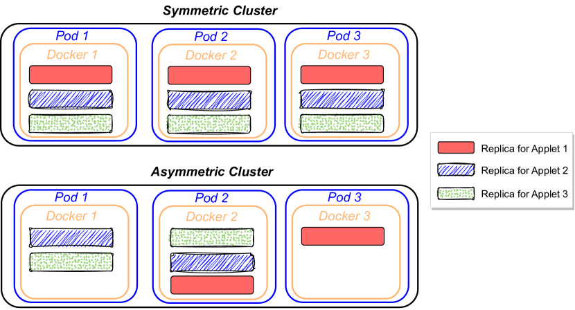
Figure 1: Schematic diagram of two common paradigms for replica deployment. Here, the ratio between the number of pods and dockers is assumed to be 1:1.

Besides, two essential rules should be noted about autoscaling in the cloud. For safety reasons, we must secure both upper and lower bounds for the number of pods in each cluster. Also, scaling in/out can be done in parallel, but the concurrency and the speed of a single pod addition/removal are limited.

3.2 Patterns of Workload and CPU Utilization

Workload prediction is an essential component in our framework, which estimates the incoming workload of various applets for future periods. In our context, the precondition for workload prediction is demonstrated in Fig. 2, which shows that the workload of many applets often exhibits periodical behaviors. Here, the applet 1 reflects a weekly pattern, while the applet 2 fluctuates daily.

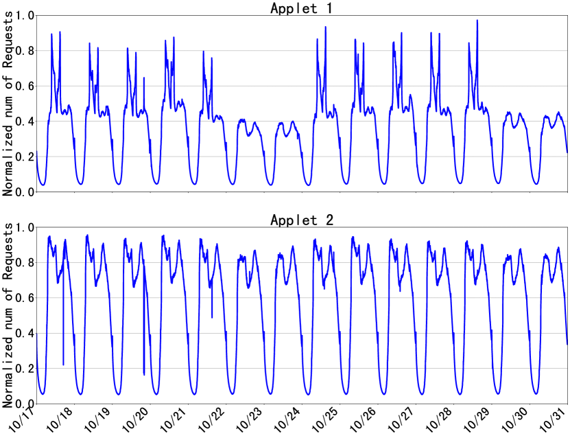
Figure 2: Periodical patterns of workload for two randomly chosen applets.

Furthermore, the mapping from workload to CPU utilization is vital for meeting the goals mentioned herein. For a better understanding of the dynamics between the workload of applets in a docker (i.e., unit workload) and the resultant CPU utilization, we first focus on the docker which solely supports one applet (referred as monopolize deployment, usually for prior applets), as it is supposed that the rule is similar for more complex mixed deployment case, where the CPU utilization is affected by all applets.

As shown in Fig. 3, in monopolize deployment case, an explicit linear correlation could be observed between unit workload and the mean value of CPU utilization. Nevertheless, Fig. 3 implies that: 1) applets vary in complexity, and the ability to impact CPU utilization varies (under the same unit workload). Here, Applet 1 is more resource-intensive than Applet 2, as under the same resource capacity of each pod and unit workload, the CPU utilization for Applet 1 is much higher than that of Applet 2 (e.g., given a workload of 40, the average CPU utilization are around 0.3 and 0.2 for Applets 1 and 2, respectively), and thus different weights should be assigned in case of a mixed deployment; 2) if a linear model is adopted for CPU utilization estimation, the residual variance will increase sharply as the unit workload increases. For leveraging the simplicity of a linear model in an optimization framework while controlling the degree of uncertainty, we propose two supplements to the vanilla linear model: a) adding an uncertain term into the linear model, which could be a distribution related to the magnitude of workload; and b) implementing an online linear regression (OLR) [40] as a feedback mechanism for real-time adaptation of the linear model itself. Instead of retraining the model using the whole dataset, the OLR directly fine-tunes the model parameters with the latest feedback data. The details of these two supplements will be provided in the following section.

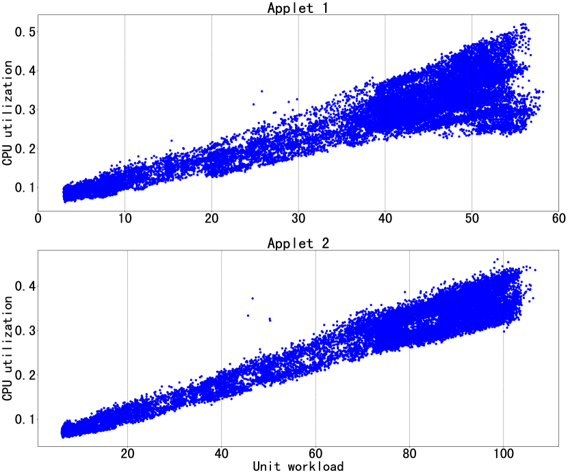
Figure 3: Scatter diagram shows a linear correlation between unit workload and CPU utilization for two randomly chosen applets.

4 Proposed Framework

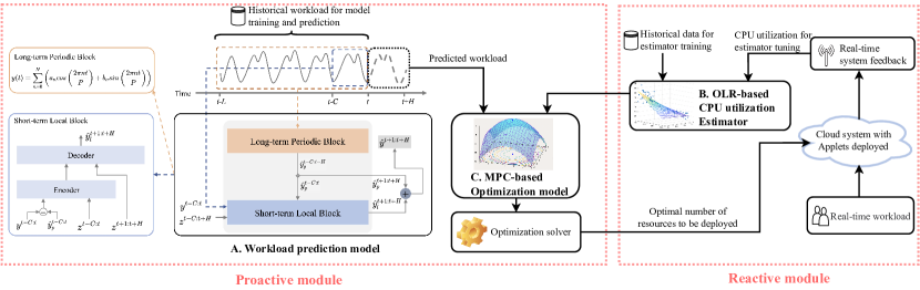
Figure 4: Flowchart of the proposed OptScaler framework.

We hereafter propose our autoscaling framework OptScaler in symmetric paradigm, mixed deployment case, as this is by far the most common context in the cloud of Alipay. For simplicity, we stipulate that the mapping relation of applet-cluster is predefined and fixed, and each pod could only install one docker. In this context, we only need to focus on the number of resource units (e.g., pods) in each cluster for making holistic scaling decisions.

The framework of OptScaler, shown in Fig. 4, consists of two modules for robust autoscaling:

• Proactive module consists of a sophisticated workload prediction model (block A) and an optimization model (block C). First, the workload prediction model is trained by the historical workload data and provides multi-timeslot predictions of future workload for all applets of concern. Then, the optimization model takes the predicted workload as input, calls a solver to output an optimal scaling decision, and sends it to the Cloud system for deployment.

• Reactive module provides a self-tuning CPU utilization estimator (block B) as another input to the optimization model. The estimator is pre-trained by the historical data of the unit workload of applets and the corresponding CPU utilization; it will continuously be tuned by the real-time system feedback under the incoming workload.

4.1 Workload Prediction Model

The workload prediction model aims to predict the future incoming workloads of different applets. The forecasting results are further provided to the MPC-based optimization model for the CPU utilization estimation and control. Since building a prediction model for each applet is infeasible, we build one model for different applets, which has much fewer parameters and is convenient for the online service.

Let $y_{n}^{t}\in\mathbb{R}$ denotes the workload value at time step $t$ of the $n$-th applet, then the workload prediction model is to predict the future values $\boldsymbol{y}_{n}^{t+1:t+H}=[y_{n}^{t+1},\ldots,y_{n}^{t+H}]$ based on its historical values $\boldsymbol{y}_{n}^{t-C:t}=[y_{n}^{t-C},\ldots,y_{n}^{t}]$ and other covariates. Note that we herein use bold symbols to denote vectors. Typically, it can be formalized as

$$\boldsymbol{y}_{n}^{t+1:t+H}=\mathcal{F}_{\Theta}(\boldsymbol{y}_{n}^{t-C:t},\boldsymbol{z}_{n}^{t-C:t+H},n)$$ (1)

where $\Theta$ is a set of learning parameters, $\boldsymbol{z}_{n}^{t-C:t+H}$ is the known covariates of the $n$-th applet, such as date, $n\in\{1,2,\ldots,N\}$ is the index of applet. It is evident that $\mathcal{F}_{\Theta}(\cdot)$ can handle the workload prediction task for various applets with the parameter $\Theta$ and distinguish different applets with their index $n$.

In order to facilitate the autoscaling, the workload predictor should consider the following problems.

• Long-term forecasting. The proposed OptScaler controls the CPU utilization by autoscaling. Due to the speed limit of pod implementation/removal and the sharp change of the workload (as shown in Fig. 2), the decision model has to consider multiple steps to handle the situation that the pod implementation/removal can not be finished in a single time interval. Therefore, we need long-term forecasting, such as predicting the workload in half a day or one day in the future.

• Different workload patterns in various applets. As shown in Fig. 2, Applet 1 reflects a weekly pattern, while Applet 2 fluctuates daily. The model $\mathcal{F}_{\Theta}(\cdot)$ has to handle this characteristic.

• Decision reliability. The underestimated workload would lead to CPU overhead, which causes degradation in system performance and long-time delays in cloud service. The predicted workload should not be lower than actual values to guarantee a reliable service.

To handle the above problems, we propose a workload prediction model shown in the left part of Fig. 4. It comprises two sub-modules: a long-term periodic block and a short-term local block.

• Long-term Periodic Block. In online services, predicting the workload through long historical data, such as the historical data in a week, is impossible. Hence, we apply the Fourier series to represent the various periodicity of different applets. For simplicity, given the parameter $P$ of periodicity and the truncation order $\hat{N}$ of Fourier series expansion, the long-term periodicity can be formalized as $y^{t}=y(t)=\sum_{n=0}^{\hat{N}}(a_{n}cos(\frac{2\pi nt}{P})+b_{n}sin(\frac{2\pi nt}{P}))$. Then, the Fourier coefficients $[a_{0},b_{0},\ldots,a_{\hat{N}},b_{\hat{N}}]$ can be learned with the historical data. And the periodicity in the future can be inferred with the time step $t$.

• Short-term Local Block. This block learns the local pattern of the workload, such as the local trend and influence. For this purpose, we apply a Seq2seq structure consisting of three steps. 1) According to the historical values $\boldsymbol{y}^{t-C:t}$ and their periodic estimation $\boldsymbol{\hat{y}}_{p}^{t-C:t}$, calculating the residual of historical series $\boldsymbol{y}_{l}^{t-C:t}=\boldsymbol{y}^{t-C:t}-\boldsymbol{\hat{y}}_{p}^{t-C:t}$. 2) Extracting the local pattern of the historical residual with the series $\boldsymbol{y}_{l}^{t-C:t}$ and the corresponding covariates $\boldsymbol{z}^{t-C:t}$. For this reason, we use the linear-complexity Flow-Attention $f(\boldsymbol{q},\boldsymbol{k},\boldsymbol{v};\boldsymbol{\theta}_{attn})$ [41], which is much more efficient for long sequences. Specifically, let $\boldsymbol{h}_{in}=[\boldsymbol{y}_{l}^{t-C:t},\boldsymbol{z}^{t-C:t}]$ denote the whole historical representation, the encoder is $\boldsymbol{h}_{enc}=f(\boldsymbol{h}_{in},\boldsymbol{h}_{in},\boldsymbol{h}_{in};\boldsymbol{\theta}_{enc})$, where $\boldsymbol{\theta}_{enc}$ is the parameters of encoder. 3) Based on the encoder output $\boldsymbol{h}_{enc}$ and the covariates $\boldsymbol{z}^{t-C:t+H}$, the decoder estimates the local residual in the future. With the same Flow-Attention structure, the decoder is $\boldsymbol{\hat{y}}_{l}^{t+1:t+H}=f(\boldsymbol{z}^{t-C:t},\boldsymbol{z}^{t+1:t+H},\boldsymbol{h}_{enc};\boldsymbol{\theta}_{dec})$, where $\boldsymbol{\theta}_{dec}$ is the learning parameter.

Two practical techniques are adopted in the short-term local block to boost long-term forecasting. One is the computationally efficient Flow-Attention. It has a linear complexity with the length of series. The other one is the non-autoregressive decoder, that is, the forecasting of time step $t$ is independent of the forecasting results of the preceding time step but only dependent on the known historical series. The non-autoregressive decoder could avoid accumulative errors and has a fast inference speed.

Finally, the forecasting workload of one applet is the summation of the estimation of long-term periodic block and short-term local block, that is

$$\boldsymbol{\hat{y}}^{t+1:t+H}=\boldsymbol{\hat{y}}_{p}^{t+1:t+H}+\boldsymbol{\hat{y}}_{l}^{t+1:t+H}$$ (2)

In the model training stage, we can adopt the quantile loss [42, 43] to reduce the ratio of the forecasting results lower than the actual values, which further improves the reliability of the subsequent decision from the workload forecasting perspective.

4.2 OLR-based CPU Utilization Estimator

A linear estimator with an uncertain term has been built to map the predicted workload of applets to the average CPU utilization of pods in the cluster, which could be formulated as follows:

$$c=f\left(\frac{\boldsymbol{y}}{x}\right)=w_{b}+\frac{\boldsymbol{y}^{\top}\boldsymbol{w}_{k}}{x}+\epsilon$$ (3)

where $f(\cdot)$ denotes the estimator; $\boldsymbol{y}\in\mathbb{R}^{N}$ is the workload for all $N$ applets; $x$ is the number of pods in the cluster to be decided; $c$ denotes the estimated CPU utilization, which is a function of unit workload $\frac{\boldsymbol{y}}{x}$; $\boldsymbol{w}_{k}$ and $w_{b}$ are the slope and intercept for the linear model, respectively. $\boldsymbol{w}_{k}$ can be seen as the weights of the applets, and $w_{b}$ is naturally the overhead load of CPU; $\epsilon$ is the uncertain term compensating for the residual of a linear model, and it obeys the following normal distribution:

$$\epsilon\sim N(0,\sigma^{2}(\frac{\boldsymbol{y}}{x}))\sim N(0,(\sigma_{b}+\frac{\boldsymbol{y}^{\top}\boldsymbol{\sigma}_{k}}{x})^{2})$$ (4)

where the standard deviation of $\epsilon$ is also modelled as a linear function (with coefficient $\boldsymbol{\sigma}_{k}$ and $\sigma_{b}$) of unit workload. In this way, we ensure that the uncertain term obeys the rules we found in Fig. 3, i.e., the variance of CPU utilization increases with larger unit workloads.

All the parameters (including $\boldsymbol{w}_{k}$, $w_{b}$, $\boldsymbol{\sigma}_{k}$ and $\sigma_{b}$) are initialized on the historical data by the maximum likelihood estimation (MLE) [44] with nonnegative constraints. As the most influential coefficient, we also adopt OLR [40] to adjust $\boldsymbol{w}_{k}$ with real-time data. Due to the feedback mechanism of OLR, it could be regarded as a supervised learning algorithm. The goal is to minimize the square loss of a linear function in an online setting. The pseudocode is shown in Algorithm 1, where $\eta$ is a parameter to control the strength of feedback tuning, in analogy with the learning rate in a Machine Learning context, and $\hat{c}^{t}-c^{t}$ is regarded as the real-time feedback from the Cloud system. In practice, after initializing $\boldsymbol{w}_{k}^{0}$ by fitting historical workload-CPU utilization data into a linear model, each time new feedback is available, we could choose the most recent (i.e., $T=1$) or a series of (i.e., $T>1$) feedback $c^{t}$, and apply OLR to update $\boldsymbol{w}_{k}$ quickly. Instead of tediously retraining the linear model using the whole dataset each time, OLR emphasized the newest $T$ feedback, and its simplicity and high efficiency become key advantages for an online system.

Algorithm 1 Widrow-Hoff algorithm for Online Linear Regression

Input: Choose parameter $\eta>0$

Initialize: $\boldsymbol{w}_{k}^{0}$ according to historical data training

for $t=1$ to $T$ do

     Get unit workload $\frac{\boldsymbol{y}^{t}}{x^{t}}$ $\in\mathbb{R}^{N}$

     Estimate $\hat{c}^{t}=f(\frac{\boldsymbol{y^{t}}}{x^{t}})\in\mathbb{R}$

     Observe $c^{t}\in\mathbb{R}$

     Update $\boldsymbol{w}_{k}^{t}=\boldsymbol{w}_{k}^{t-1}-\eta(\hat{c}^{t}-c^{t})\frac{\boldsymbol{y^{t}}}{x^{t}}$

end for

return $\boldsymbol{w}_{k}^{t}$

4.3 MPC-based Optimization Model

We employ MPC to repeatedly solve a constrained optimization model at every $h-$minute interval for corresponding autoscaling decisions. If a scaling decision is made at time step $t$, the next scaling decision will be made at $t+h$. Upon making the scaling decision for each cluster $i\in\{1,2,\ldots,I\}$ at $t$, the workloads in future $D$ timeslots are considered. Each timeslot, indexed by $d\in\{1,2,\ldots,D\}$, spans $h$ minutes (e.g., 30 minutes) that can be much longer than the resolution of workload predictions (e.g., 1 minute). Within the optimization model of $D$ timeslots, the initial number of pods $x_{i}^{0}$ takes the value of $x_{i}^{t}$ to capture the latest number of pods deployed at $t$, and the predicted workload $\boldsymbol{y}_{i}^{d}$ and the CPU utilization estimator $f(\cdot)$ are given as input. Then, the following optimization model is established:

$$\min_{\boldsymbol{u}}\quad \sum_{i=1}^{I}\sum_{d=1}^{D}\left(|c_{i}^{d}-c_{i}^{*}|\right)$$ (5)

$$s.t.\quad |u_{i}^{d}|\leq\frac{h}{\tau}\cdot s, \forall i,d$$ (6)

$$x_{i}^{d}=x_{i}^{0}+\sum_{j=1}^{d}u_{i}^{j}, \forall i,d$$ (7)

$$c_{i}^{d}=\max_{j\in\{d,d+1\}}f\left(\frac{\boldsymbol{y}_{i}^{j}}{x_{i}^{d}}\right), \forall i,d$$ (8)

$$c_{i}^{d}\leq c_{i}^{*}, \forall i,d$$ (9)

$$X_{i}^{min}\leq x_{i}^{d}\leq X_{i}^{max}, \forall i,d$$ (10)

where $u_{i}^{d}$ is the only decision variable that denotes the change of number of pods of cluster $i$ in timeslot $d$, and $\boldsymbol{u}=[u_{1}^{1},\ldots,u_{I}^{D}]\in\mathbb{R}^{I\times D}$ is the vector that collects all these variables. A positive $u_{i}^{d}$ increases the pod number while a negative $u_{i}^{d}$ decreases it. Only the solution in the first timeslot, $u_{i}^{1}$, is returned for deployment.

The objective (5) is to keep the resulting system indicators (CPU utilization) at a desired level. Specifically, for each cluster $i$, we minimize the total deviation between the peak value of average CPU utilization $c_{i}^{d}$ at each timeslot $d$ and the desirable one $c_{i}^{*}$. The constraints for cluster $i$ are explained as follows:

• Constraint (6): the speed limitation of scaling, where $h$ (the span of a timeslot) is the time interval between two successive scaling actions. $\tau$ and $s$ denote the time cost of a single pod addition/removal and the concurrency of scaling actions, respectively;

• Constraint (7): the state transition equation that describes the relationship between the system’s number of pods $x_{i}^{d}$ at $d$ and the input $x_{i}^{0}$, the initial number of pods;

• Constraints (8): The estimator $f(\cdot)$ have been introduced in Section 4.2, and $\boldsymbol{y_{i}^{j}}$ is the vector denoting the predicted peak workload of $N$ applets of cluster $i$ in timeslot $j\in\{d,d+1\}$. Note that for each timeslot $d$, $c_{i}^{d}$ is estimated as the maximum CPU utilization in two adjacent timeslots {$d,d+1$}. This is because we always make scaling decisions in advance (i.e., the resource for timeslot $d+1$ is provisioned one timeslot ahead at $d$), and for safety reasons, the decision should be prepared for workload in both the incoming timeslot and the timeslot after that;

• Constraint (9): the peak CPU utilization $c_{i}^{d}$ is upper bounded by $c_{i}^{*}$;

• Constraint (10): the upper and lower bounds for the number of pods in each cluster.

Due to uncertainty in $f(\cdot)$, constraint (9) is easily violated. To derive a robust solution, we reformulate constraints (8) and (9) by chance constraint (11) that guarantees satisfaction of constraint (9) with probability $\alpha$:

$$\mathbb{P}\{c_{i}^{*}\geq c_{i}^{d}=\max_{j\in\{d,d+1\}}f\left(\frac{\boldsymbol{y}_{i}^{j}}{x_{i}^{d}}\right)\}\geq\alpha,\quad\forall i,d$$ (11)

Consider the formulation of $f(\cdot)$ in (3), constraint (11) can be converted to a deterministic equivalent form under the theory of chance-constraint method [15]:

$$c_{i}^{*}\geq c_{i}^{d} =\frac{1}{x_{i}^{d}}\max_{j\in\{d,d+1\}}(\psi^{-1}(\alpha)\cdot{\boldsymbol{\sigma}_{k,i}}+{\boldsymbol{w}_{k,i}})^{\top}\boldsymbol{y}_{i}^{j}$$

$$+w_{b,i}+\psi^{-1}(\alpha)\cdot\sigma_{b,i},\hskip 63.16515pt\forall i,d$$ (12)

where $\psi^{-1}(\cdot)$ is the inverse of the cumulative distribution function of a standard normal distribution. For example, $\psi^{-1}(\alpha)\approx 1.28$ when $\alpha=0.9$. Define $m_{i}^{d}=\max_{j\in\{d,d+1\}}(\psi^{-1}(\alpha)\cdot{\boldsymbol{\sigma}_{k,i}}+{\boldsymbol{w}_{k,i}})^{\top}\boldsymbol{y}_{i}^{j}$, which can be calculated before solving the optimization model, constraint (4.3) can be rearranged to an equivalent linear form by simple algebraic calculation:

$$x_{i}^{d}\geq\frac{m_{i}^{d}}{c_{i}^{*}-w_{b,i}-\psi^{-1}(\alpha)\cdot\sigma_{b,i}}.\hskip 39.83368pt\forall i,d$$ (13)

Constraint (4.3) also restricts $c_{i}^{d}$ from exceeding $c^{*}_{i}$, hence, by omitting constant terms, objective (5) is equivalent to

$$\max_{\boldsymbol{u}}\quad\sum_{i=1}^{I}\sum_{d=1}^{D}\frac{m_{i}^{d}}{x_{i}^{d}}.$$ (14)

Now the optimization problem (5)-(10) under uncertainty is readily reformulated to a robust counterpart with non-linear objective (14) and linear constraints (6), (7), (10), (13), which can be solved by off-the-shelf solvers (e.g. IPOPT) and the solution (number of pods in each cluster) can be rounded for implementation.

5 Numerical Results

We empirically validate the performance of the proposed OptScaler. As a hybrid autoscaler, both proactive and reactive modules are involved, and there is no doubt that the improvement of each module will benefit the whole framework. Here arises the following questions:

• Question 1: How do we demonstrate the superiority of our workload prediction model over other prevalent prediction models?

• Question 2: Except for a better prediction model, what advantages does OptScaler have compared to mainstream autoscaling frameworks, i.e., reactive, proactive, and existing hybrid frameworks?

• Question 3: When we combine the above two sides of the coin, how much is the overall advantage of OptScaler compared to the state-of-the-art autoscaler in the scenario of online services?

In this section, we explicitly answer all these three questions by analyzing the numerical experiment results.

5.1 Dataset and Experiment Settings

5.1.1 Dataset

In order to evaluate and analyze different autoscalers, we conduct experiments on the public dataset of MS Azure Functions Trace [45]. The invocation counts data of two functions (unique hash id ends with 4b3e and 8df4, respectively) are extracted from the Trace, with a duration of two weeks (from July/15/2019 to July/28/2019) and a minute-level resolution. The workloads of these two functions are representative of online services with a daily return period, and the number and occurrence time of their peaks are also different, which makes the selected dataset challenging enough to differentiate the proposed framework from previous autoscalers. We assume that these two functions are deployed as applets in a symmetric paradigm, mixed deployment case. The corresponding time series of invocation counts data are shown in Fig. 5. Furthermore, due to the lack of historical data on CPU utilization, we apply two different sets of dummy coefficients of $f$ (i.e., $\boldsymbol{w}_{k}$ and $w_{b}$ in (3), $\boldsymbol{\sigma}_{k}$ and $\sigma_{b}$ in (4)) to generate the real feedback of CPU utilization.

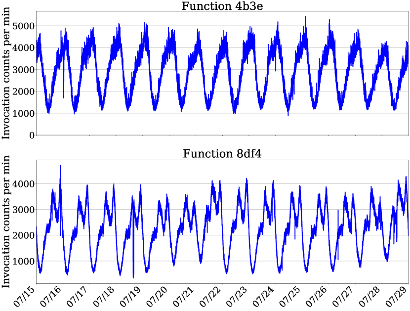
Figure 5: Time series of invocation counts for the two selected Azure Functions.

5.1.2 Experiment Settings

We imitate the actual usage of the proposed autoscaling framework to implement the experiments. The OptScaler will be triggered periodically to control the CPU utilization. In more detail, we imitate the autoscaling process for $3$ days from Jul/26 to Jul/28, and make the scaling decisions every half hour (i.e., $h=30$ minutes as the time interval between two successive scaling actions) to approach the target CPU utilization $c_{i}^{*}=0.5$. Regarding the proactive and hybrid autoscaling frameworks, the predictions of the future invocation counts should be provided by workload prediction models for the scaling decisions, which can be trained on the data before the trigger time. Furthermore, we consider the scaling speed, determined by the time cost $\tau$ of a single pod addition/removal and the concurrency of scaling actions $s$ in (6). The obtained decisions cannot be completed instantly, significantly influencing the rapidly growing/decreasing intervals. We set $\tau=5$ minutes and $s=4$ according to the real condition. Given $h=30$ minutes, a max of 24 pods could be added/removed in each timeslot. Besides, we ascertain the bound of the number of pods $X_{i}^{min}=80$ and $X_{i}^{max}=350$ for all cluster $i$ and experiment groups.

5.2 Comparison of Workload Prediction Models

5.2.1 Prediction Models

To answer Question 1, we compare our workload prediction model with several traditional and state-of-the-art time series prediction models, including ARIMA [46], Autoformer [47], NBEATS [48], and DEPTS [49]. ARIMA is a traditional time series prediction model in statistics. Due to the workload pattern in Section 3.2, we adopt ARIMA with the exogenous regressors of the Fourier series. Autoformer is a neural network model for long-term prediction based on the time series auto-correlation mechanism and seq2seq structure. NBEATS and DEPTS are two types of neural networks for the univariate times series prediction problem based on the neural expansion analysis method. In the rolling window experiment, we train the ARIMA model every half hour with the latest data in one day due to its fast training speed. We train the model at midnight each day for the neural network-based models. In each training process, the data before the training time are the training dataset, while the last two days are adopted for validation. All these neural network-based models are trained with the $0.5$-quantile loss (i.e., MAE loss).

5.2.2 Evaluation Metrics

We compare different models in terms of the long-term prediction performance, that is, giving the predictions of the following $360$ minutes every half hour. Two evaluation metrics are adopted to compare different models, including mean absolute percentage error, abbreviated as mape, and weighted absolute percentage error, abbreviated as wape, which can be formalized as follows,

$$mape =\frac{1}{N}\sum_{n=1}^{N}\frac{1}{|\Omega|}\sum_{(t,\delta)\in\Omega}\frac{|y_{n}^{t+\delta}-\hat{y}_{n}^{t+\delta}|}{|y_{n}^{t+\delta}|}$$ (15)

$$wape =\frac{1}{N}\sum_{n=1}^{N}\frac{\sum_{(t,\delta)\in\Omega}|y_{n}^{t+\delta}-\hat{y}_{n}^{t+\delta}|}{\sum_{(t,\delta)\in\Omega}|y_{n}^{t+\delta}|}$$ (16)

where $n$ is the index of the time series (also the index of the applet in our experiments) in the dataset. $t$ is the starting time step of each testing rolling window, and $\delta\in[0,359]$ is the relative position index in each rolling window, that is, $(t,\delta)$ means the $\delta$-th step after the starting time $t$ of the rolling window. $\Omega$ denotes the whole evaluation space of every time series. Note that $wape$ can be treated as the weighted version of $mape$, and the weight is the true value $y_{n}^{t+\delta}$. So, the larger the true value, the greater the influence on $wape$.

We evaluate the experimental models in two aspects. 1) One is the analysis of the Minute-value level results, that is, whether the model can accurately predict the workload of each applet in each minute, since all the models are built on the data recorded every minute. 2) The other one analyzes the Interval-peak level results. In the MPC-based optimization model, $\boldsymbol{y}_{i}^{j}\in\mathbb{R}^{N}$ in constraint (8) is the interval peak of the prediction results. Therefore, the accuracy of the predicted Interval-peak is also critical to the subsequent optimization model. In our experiments, we calculate the peak value in each no-overlapping $30$ minutes of the prediction results and ground truth, which is consistent with the usage of the optimization model.

5.2.3 Experimental Results for Question 1

Table 2: Performance comparisons on five workload prediction models testing on $mape$ and $wape$, in terms of two perspectives, including the analyses of Minute-value and Interval-peak. Lower is better, and the best is in bold.

	Minute-value level		Interval-peak level
	$mape$	$wape$	$mape$	$wape$
ARIMA	0.0903	0.0871	0.1125	0.1068
Autoformer	0.0902	0.0795	0.0927	0.0853
DEPTS	0.0709	0.0664	0.0860	0.0816
NBEATS	0.0712	0.0666	0.0903	0.0855
Our model	0.0660	0.0628	0.0859	0.0798

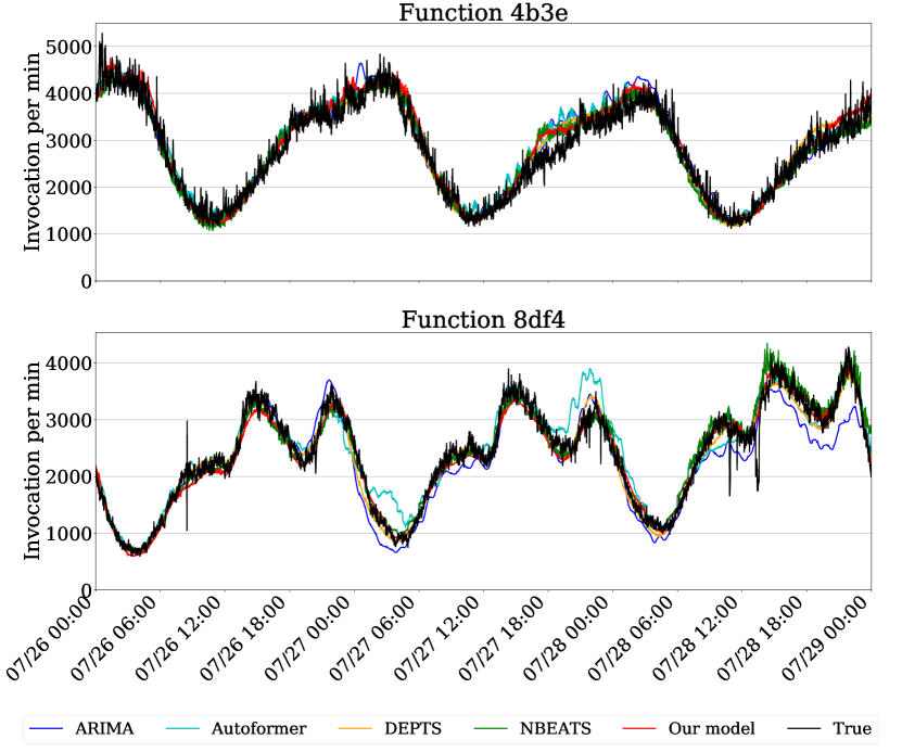
Figure 6: Comparison of five workload prediction models based on Azure Functions in Fig. 5.

Table 2 shows the experimental results of five prediction models, testing on $mape$ and $wape$ in terms of two perspectives. No matter on the minute-value level analysis or the interval-peak level analysis, our model has better performance than ARIMA with a large margin. It verifies the effectiveness of the short-term local block in our model, since both ARIMA and our model extract the periodic property with the Fourier series. Meanwhile, our model is superior to all compared models at the minute-value level. In the interval-peak level, our model is on par with DEPTS and performs better than others. Compared with DEPTS, our model can handle multiple time series by one model with fewer parameters, which is much more suitable for the online autoscaling framework with multiple time series.

Fig. 6 illustrates the predicted time series of each model as well as the true workload for our testing period (from Jul/26 to Jul/28). As all the models are doing long-term prediction with a rolling window strategy, each predicted series in Fig. 6 is presented by averaging over multiple predictions, which is also practical. Both ARIMA and Autoformer fail to capture specific temporal patterns of the True series, especially in the more complex case of Function 8df4 from Jul/27 to Jul/28. NBEATS tends to overestimate the peaks in Jul/28, and DEPTS tends to underestimate the bottom. Instead, our model closely follows the rise and fall of the True series of Function 8df4, as it can capture complex patterns with daily and weekly periodic dependencies.

5.3 Comparison of Autoscaling Frameworks

In this section, we conduct an ablation experiment to compare the performance of OptScaler with prevalent autoscaling frameworks in the scenario of online services. Specifically, we respond to Question 2 by testing all the frameworks under the same input of prediction results; then, we address Question 3 by comparing OptScaler with the best combination of the existing prediction model and framework.

5.3.1 Autoscaling Frameworks

We investigate four autoscaling frameworks, i.e., reactive, proactive, hybrid, and OptScaler. Below are the details:

• Autopilot [6] is selected as the representative of reactive autoscalers. Proposed by Google in 2020, it is introduced as an industrial benchmark here. Autopilot decides the optimal resource configuration by seeking the best-matched historical timeslot to the current window. We implement Autopilot’s horizontal scaling based on its public paper [6];

• Madu [21] is a typical proactive autoscaler, which adopts the power of both prediction and optimization models. We adapt Madu to our context, where the optimization model is formulated as (5) to (10). As a pure proactive autoscaler, the CPU utilization estimator will not be updated after initialization;

• HAS [27] is a hybrid autoscaler that follows the mainstream idea of hybrid works that the proactive and reactive modules work independently. We transfer HAS to our context, where the reactive decision replaces the proactive one when the observed CPU utilization exceeds a predefined bound. The current bound is set to be $0.9c^{*}_{i}$. The reactive decision at current time $t$ is calculated by $u_{i}^{t}=\max\{X^{min}_{i}-x_{i}^{t-1},\ \min\{(c_{i}^{t-1}/c^{*}_{i}-1)x_{i}^{t-1},\ hs/\tau,\ X^{max}_{i}-x_{i}^{t-1}\}\}$. The $\min$ operation indicates $c_{i}^{t}\leq c^{*}_{i}$ if the current workload does not increase, the $\max$ operation guarantees the lower bound in (10) holds.

• OptScaler is our proposed hybrid framework.

Besides, we also customize the following parameters for the frameworks:

• $S$ represents the most recent CPU utilization samples for Autopilot. A higher $S$ denotes a more conservative scaling preference. Here we try two different $S\in\{90\%,95\%\}$;

• $D$ is the time horizon for Madu, HAS, and OptScaler. In our context, we use $h=30$ for each timeslot $d$, and $D=1$ is adopted to represent a standard optimization model focusing on immediate scaling needs, while $D=6$ for an MPC-based optimization model that can anticipate what happens in the following 3-hour;

• $\eta$ is the parameter to control the strength of feedback tuning in OLR. We adopt $\eta=1e-4$ for HAS and OptScaler. $\eta$ is chosen by minimizing the cumulative loss of Algorithm 1 in the historical dataset;

• Besides, we set the parameter of the chance constraint as $\alpha=0.95$ for all optimization-based frameworks.

5.3.2 Evaluation Metrics

Table 3: Evaluation metrics for the investigated autoscaling frameworks

Symbol	Gist	Measurement
$r_{e}$a	Reliability	The violation rate of maximal CPU utilization during the experiment
$c_{avg}$a	CPU utilization	The average CPU utilization during the experiment
$e_{avg}$b	Expenditure	The average number of installed resource units during the experiment

• Higher is better;

• Lower is better.

As an end-to-end autoscaling framework, our prior goal is to maintain key system indicators (i.e., average CPU utilization of dockers under the synergistic effect of all the deployed replicas) of each cluster at a desired level, where a higher level brings risk (low reliability), and a lower level implies a waste of resources/money (low efficiency). Based on this goal, three useful metrics have been developed and illustrated in Table 3.

5.3.3 Experimental Results for Question 2

Table 4: Performance comparison on the investigated autoscalers based on the metrics in Table 3, under the same input of prediction results.

Type	Name	Parameter	$r_{e}$a	$e_{avg}$a	$c_{avg}$a
Reactive	Autopilot	$S=90\%$	0.939	115.88	0.385
		$S=95\%$	0.972	119.02	0.377
Proactive	Madu	$D=1$	0.847	90.30	0.437
		$D=6$	0.850	90.70	0.436
Hybrid	HAS	$D=1$	0.968	105.76	0.421
		$D=6$	0.976	106.50	0.412
Hybrid	OptScaler	$D=1$	0.992	116.32	0.383
	(proposed)	$D=6$	0.993	114.60	0.387

• Due to the randomness in the sampling of CPU utilization feedback, all metrics are averaged over five repetitive runs and calculated at a minute interval.

The overall statistic results are summarized in Table 4, where the metrics are explained in Table 3. From Table 4, it is clear that:

• Autopilot achieves a decent performance in reliability, especially under the highest quantile of $S=95$ with $r_{e}=0.972$. In contrast, the overall resource costs of Autopilot $e_{avg}$ is 119.02 (the highest among experiment groups), which results in a relatively low $c_{avg}$.

• Madu shows the lowest satisfaction rate of Constraint (9). With $r_{e}<0.9$, the cluster will take a high risk of SLO violations, which could be explained by the gap between the estimation of CPU utilization and the real feedback. Without the adjustment from the reactive module, this gap will continually undermine the reliability of final scaling decisions. Again, this encapsulates the statement of [12] that a reactive scaling component should be a part of every production-ready autoscaler as a complement to an unsatisfied proactive counterpart.

• OptScaler outperforms Autopilot concerning both reliability and resource costs. The average cost $e_{avg}$ of OptScaler is somewhat higher (7% $\sim$ 10%) than that of HAS under the same $D$, while the former performs much better in $r_{e}$.

• Based on the comparisons between $D=1$ and $D=6$ in each type, the multi-timeslots optimization structure in MPC could bring an extra improvement of $r_{e}$.

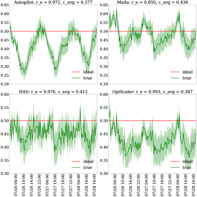
Figure 7: CPU utilization for the four typical experiment groups in Table 4.

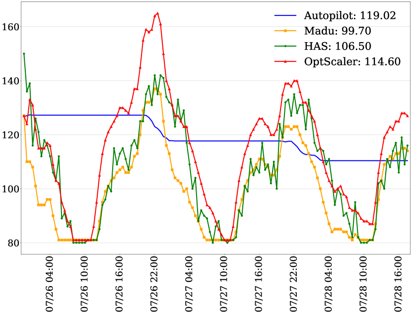
Figure 8: Expenditure for the four typical experiment groups in Table 4.

We construct Fig. 7 and 8 to provide further experimental details. For clarity, we only focus on four typical experiment groups in Table 4, i.e., with $S=95\%$ for Autopilot and $D=6$ for the rest optimization-based groups. Here, Fig. 7 and 8 focus on the fluctuation of CPU utilization and number of pods during the whole experimental period, respectively.

In Fig. 7, we do the ideal and true CPU utilization line plots. The shallow green area around each point in the true series denotes the $\alpha=0.95$ confidence interval of the true CPU utilization. It is notable that:

• Without the power of workload prediction, Autopilot suffers from drastic fluctuations in CPU utilization, which is synchronized with the trend of total workload (invocations of two functions).

• Madu shows the highest risk of exceeding the bound of $c_{i}^{*}$ (the red line), and the magnitude of violation (and thus the severity) is also higher than other experiment groups, due to the lack of adjustment from a reactive module.

• HAS and OptScaler show similarities in the overall trend, whereas the proposed OptScaler stands out with a smoother and more robust trend. During the night, when the total workload is relatively high, OptScaler could keep CPU utilization at a safer range, and the magnitude of violations is lower than that of HAS.

On the other hand, Fig. 8 shows a reversed trend of expenditure fluctuations among the frameworks, where Autopilot outputs a much flatter scaling plan. That is what we expected based on the hysteretic nature of a reactive autoscaler. Another observation worth mentioning is that, when compared with Madu and HAS, when the total workload is relatively high, the proposed OptScaler tends to add a couple of pods, contributing to better efficiency and reliability of the framework.

5.3.4 Experimental Results for Question 3

As stated at the beginning of this section, we believe that OptScaler benefits from improving the workload prediction model and autoscaling framework. To address the related Question 3, we compare OptScaler with the existing framework of DEPTS (the second-best prediction model in Table 2) plus HAS (the second-best framework in Table 4). Furthermore, we also adopt DEPTS to replace the workload prediction model in our proposed OptScaler to illustrate the influence of different prediction models on the final autoscaling decision. The results are shown in Table 5, which calculates the same way as Table 4. Comparing the Exp.2 to Exp.1 in Table 5, we gain a 1.7% improvement of $r_{e}$ by upgrading the autoscaling framework alone. A further 0.2% improvement of $r_{e}$ (as well as 0.2% saving of $e_{avg}$) needs to be obtained by advancing the prediction model (comparing the Exp.3 to Exp.2 in Table 5).

Table 5: Comparison between OptScaler and an existing hybrid framework in an ablative way

Experiment group	Workload prediction model	Autoscaling framework	$r_{e}$	$e_{avg}$	$c_{avg}$
Exp.1	DEPTS	HAS	0.974	106.54	0.412
Exp.2	DEPTS	OptScaler	0.991	114.79	0.386
Exp.3	Our model	OptScaler	0.993	114.60	0.387

6 Deployment

The proposed framework OptScaler has been successfully deployed on the cloud cluster at Alipay, supporting the autoscaling of more than 100 online applet services. The progress is based on an experiment conducted in a mixed deployment cluster (with three applets) of Alipay, which verifies the effectiveness of OptScaler in an online environment. Before we experiment, no scaling strategy was applied on the cluster, and the number of pods was fixed at a relatively high level (here 210), which is a baseline to be optimized. We decided not to compare OptScaler with other frameworks due to the concern that the latter will cause violations of SLOs with a probability of over 2%, which is indicated by Fig. 7.

The result of the experiment for the entire day of Aug/22 is shown in Fig. 9. OptScaler achieves a steady CPU utilization during a long daily time, from 7 am to around 10 pm, which is also closer to the $c^{*}$ (denoted as Ideal) than the baseline method (denoted as Constant). The overall $c_{i}^{*}$ has been improved from 0.307 to 0.342 (increased by 11.4%). Besides, with an average Expenditure of 170 pods, we save 19% of resources than Constant. The reason for low CPU utilization from 0 am to 6 am is that, for safety, we set a fixed lower bound of the number of pods $X_{i}^{min}=150$, which is well above the workload requirement overnight. Specifically, the nightly workload load is only 1/10 of that in daily times, and the major contributor to CPU utilization is the overhead load $w_{b}$ in (3).

7 Conclusion

We propose OptScaler, a hybrid proactive-reactive framework for autoscaling. To the best of our knowledge, OptScaler is the first framework that leverages optimization techniques (e.g., MPC) in a hybrid autoscaler. Instead of using proactive and reactive methods independently to avoid incompatibilities, OptScaler absorbs the strengths of both proactive and reactive modules to encounter system uncertainty and prediction deviations, thus significantly improving robustness. OptScaler effectively stabilizes applets’ CPU utilization and saves cloud resources in both offline and online experiments. OptScaler has been deployed online at Alipay to support the autoscaling of applets in the world-leading payment platform.

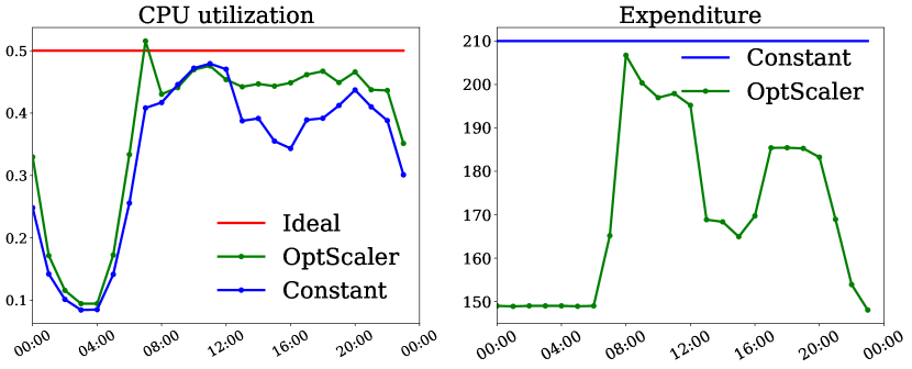
Figure 9: Online experimental results of OptScaler testing on CPU utilization and expenditure.

Ethical Statement

There are no ethical issues.

IEEEexample:BSTcontrol MyBSTcontrol

References

- [1] J. Ding, R. Cao, I. Saravanan, N. Morris, and C. Stewart, “Characterizing service level objectives for cloud services: Realities and myths,” in 2019 IEEE International Conference on Autonomic Computing (ICAC). IEEE, 2019, pp. 200–206.
- [2] T. Chen, R. Bahsoon, and X. Yao, “A survey and taxonomy of self-aware and self-adaptive cloud autoscaling systems,” ACM Computing Surveys (CSUR), vol. 51, no. 3, pp. 1–40, 2018.
- [3] S. Farokhi, P. Jamshidi, E. B. Lakew, I. Brandic, and E. Elmroth, “A hybrid cloud controller for vertical memory elasticity: A control-theoretic approach,” Future Generation Computer Systems, vol. 65, pp. 57–72, 2016.
- [4] Z. Zhou, C. Zhang, L. Ma, J. Gu, H. Qian, Q. Wen, L. Sun, P. Li, and Z. Tang, “Ahpa: Adaptive horizontal pod autoscaling systems on alibaba cloud container service for kubernetes,” arXiv preprint arXiv:2303.03640, 2023.
- [5] Y. Al-Dhuraibi, F. Paraiso, N. Djarallah, and P. Merle, “Elasticity in cloud computing: state of the art and research challenges,” IEEE Transactions on Services Computing, vol. 11, no. 2, pp. 430–447, 2017.
- [6] K. Rzadca, P. Findeisen, J. Świderski, P. Zych, P. Broniek, J. Kusmierek, P. K. Nowak, B. Strack, P. Witusowski, S. Hand, and J. Wilkes, “Autopilot: Workload autoscaling at google scale,” in Proceedings of the Fifteenth European Conference on Computer Systems, 2020. [Online]. Available: https://dl.acm.org/doi/10.1145/3342195.3387524
- [7] H. Qiu, S. S. Banerjee, S. Jha, Z. T. Kalbarczyk, and R. K. Iyer, “FIRM: An intelligent fine-grained resource management framework for SLO-Oriented microservices,” in 14th USENIX symposium on operating systems design and implementation (OSDI 20), 2020, pp. 805–825.
- [8] A. Gambi, W. Hummer, H.-L. Truong, and S. Dustdar, “Testing elastic computing systems,” IEEE Internet Computing, vol. 17, no. 6, pp. 76–82, 2013.
- [9] V. Podolskiy, A. Jindal, and M. Gerndt, “Iaas reactive autoscaling performance challenges,” in 2018 IEEE 11th International Conference on Cloud Computing (CLOUD). IEEE, 2018, pp. 954–957.
- [10] N. Dezhabad and S. Sharifian, “Learning-based dynamic scalable load-balanced firewall as a service in network function-virtualized cloud computing environments,” The Journal of Supercomputing, vol. 74, no. 7, pp. 3329–3358, 4 2018.
- [11] S. Xue, C. Qu, X. Shi, C. Liao, S. Zhu, X. Tan, L. Ma, S. Wang, S. Wang, Y. Hu et al., “A meta reinforcement learning approach for predictive autoscaling in the cloud,” in Proceedings of the 28th ACM SIGKDD Conference on Knowledge Discovery and Data Mining, 2022, pp. 4290–4299.
- [12] M. Straesser, J. Grohmann, J. von Kistowski, S. Eismann, A. Bauer, and S. Kounev, “Why is it not solved yet? challenges for production-ready autoscaling,” in Proceedings of the 2022 ACM/SPEC on International Conference on Performance Engineering, 2022, pp. 105–115.
- [13] K. Holkar and L. M. Waghmare, “An overview of model predictive control,” International Journal of control and automation, vol. 3, no. 4, pp. 47–63, 2010.
- [14] S. Burroughs, H. Dickel, M. van Zijl, V. Podolskiy, M. Gerndt, R. Malik, and P. Patros, “Towards autoscaling with guarantees on kubernetes clusters,” in 2021 IEEE International Conference on Autonomic Computing and Self-Organizing Systems Companion (ACSOS-C), 2021, pp. 295–296.
- [15] A. Shapiro, D. Dentcheva, and A. Ruszczynski, Lectures on stochastic programming: modeling and theory. SIAM, 2021.
- [16] S. Wang, Y. Sun, X. L. Shi, S. Zhu, L. Ma, J. Zhang, Y. Zheng, and J. Liu, “Full scaling automation for sustainable development of green data centers,” in International Joint Conference on Artificial Intelligence, 2023. [Online]. Available: https://api.semanticscholar.org/CorpusID:258426715
- [17] N. Roy, A. Dubey, and A. Gokhale, “Efficient autoscaling in the cloud using predictive models for workload forecasting,” in 2011 IEEE 4th International Conference on Cloud Computing. IEEE, 2011, pp. 500–507.
- [18] P. Jamshidi, C. Pahl, and N. C. Mendonça, “Managing uncertainty in autonomic cloud elasticity controllers,” IEEE Cloud Computing, vol. 3, no. 3, pp. 50–60, 2016.
- [19] Q. Zhang, Q. Zhu, M. F. Zhani, R. Boutaba, and J. L. Hellerstein, “Dynamic service placement in geographically distributed clouds,” IEEE Journal on Selected Areas in Communications, vol. 31, no. 12, pp. 762–772, 2013.
- [20] H. Qian, Q. Wen, L. Sun, J. Gu, Q. Niu, and Z. Tang, “Robustscaler: Qos-aware autoscaling for complex workloads,” in 2022 IEEE 38th International Conference on Data Engineering (ICDE). IEEE, 2022, pp. 2762–2775.
- [21] S. Luo, H. Xu, K. Ye, G. Xu, L. Zhang, G. Yang, and C. Xu, “The power of prediction: Microservice auto scaling via workload learning,” in Proceedings of the 13th Symposium on Cloud Computing, ser. SoCC ’22. New York, NY, USA: Association for Computing Machinery, 2022, p. 355–369. [Online]. Available: https://doi.org/10.1145/3542929.3563477
- [22] Z. Pan, Y. Wang, Y. Zhang, S. B. Yang, Y. Cheng, P. Chen, C. Guo, Q. Wen, X. Tian, Y. Dou et al., “Magicscaler: Uncertainty-aware, predictive autoscaling,” Proceedings of the VLDB Endowment, vol. 16, no. 12, pp. 3808–3821, 2023.
- [23] M. Gaggero and L. Caviglione, “Model predictive control for energy-efficient, quality-aware, and secure virtual machine placement,” IEEE Transactions on Automation Science and Engineering, vol. 16, no. 1, pp. 420–432, 2018.
- [24] V. Persico, D. Grimaldi, A. Pescape, A. Salvi, and S. Santini, “A fuzzy approach based on heterogeneous metrics for scaling out public clouds,” IEEE Transactions on Parallel and Distributed Systems, vol. 28, no. 8, pp. 2117–2130, 2017.
- [25] B. Urgaonkar, P. Shenoy, A. Chandra, P. Goyal, and T. Wood, “Agile dynamic provisioning of multi-tier internet applications,” ACM Transactions on Autonomous and Adaptive Systems (TAAS), vol. 3, no. 1, pp. 1–39, 2008.
- [26] A. Ali-Eldin, J. Tordsson, and E. Elmroth, “An adaptive hybrid elasticity controller for cloud infrastructures,” in 2012 IEEE Network Operations and Management Symposium. IEEE, 2012, pp. 204–212.
- [27] B. B. JV and D. Dharma, “Has: hybrid auto-scaler for resource scaling in cloud environment,” Journal of Parallel and Distributed Computing, vol. 120, pp. 1–15, 2018.
- [28] P. Singh, A. Kaur, P. Gupta, S. S. Gill, and K. Jyoti, “Rhas: robust hybrid auto-scaling for web applications in cloud computing,” Cluster Computing, vol. 24, no. 2, pp. 717–737, 2021.
- [29] Amazon, “Dynamic scaling for amazon ec2 auto scaling,” https://docs.aws.amazon.com/autoscaling/ec2/userguide/as-scale-based-on-demand.html, 2023.
- [30] Microsoft, “Overview of autoscale in azure,” https://learn.microsoft.com/en-us/azure/azure-monitor/autoscale/autoscale-overview, 2023.
- [31] P. Singh, P. Gupta, K. Jyoti, and A. Nayyar, “Research on auto-scaling of web applications in cloud: survey, trends and future directions,” Scalable Computing: Practice and Experience, vol. 20, no. 2, pp. 399–432, 2019.
- [32] V. Rampérez, J. Soriano, D. Lizcano, and J. A. Lara, “Flas: A combination of proactive and reactive auto-scaling architecture for distributed services,” Future Generation Computer Systems, vol. 118, pp. 56–72, 2021.
- [33] Y. Ogawa, G. Hasegawa, and M. Murata, “Hierarchical and frequency-aware model predictive control for bare-metal cloud applications,” in 2018 IEEE/ACM 11th International Conference on Utility and Cloud Computing (UCC). IEEE, 2018, pp. 11–20.
- [34] H. Ghanbari, M. Litoiu, P. Pawluk, and C. Barna, “Replica placement in cloud through simple stochastic model predictive control,” in 2014 IEEE 7th International Conference on Cloud Computing. IEEE, 2014, pp. 80–87.
- [35] E. Incerto, M. Tribastone, and C. Trubiani, “Combined vertical and horizontal autoscaling through model predictive control,” in Euro-Par 2018: Parallel Processing: 24th International Conference on Parallel and Distributed Computing, Turin, Italy, August 27-31, 2018, Proceedings 24. Springer, 2018, pp. 147–159.
- [36] T. De Matteis and G. Mencagli, “Proactive elasticity and energy awareness in data stream processing,” Journal of Systems and Software, vol. 127, pp. 302–319, 2017.
- [37] ——, “Keep calm and react with foresight: Strategies for low-latency and energy-efficient elastic data stream processing,” ACM SIGPLAN Notices, vol. 51, no. 8, pp. 1–12, 2016.
- [38] Kubernetes, “Kubernetes documentation / reference / glossary,” https://kubernetes.io/docs/reference/glossary/?all=true#term-cluster, 2023.
- [39] ——, “Kubernetes documentation / concepts / containers,” https://kubernetes.io/docs/concepts/containers/, 2023.
- [40] M. Mohri, A. Rostamizadeh, and A. Talwalkar, Foundations of machine learning. MIT press, 2018.
- [41] H. Wu, J. Wu, J. Xu, J. Wang, and M. Long, “Flowformer: Linearizing transformers with conservation flows,” arXiv preprint arXiv:2202.06258, 2022.
- [42] Y. Park, D. Maddix, F.-X. Aubet, K. Kan, J. Gasthaus, and Y. Wang, “Learning quantile functions without quantile crossing for distribution-free time series forecasting,” in International Conference on Artificial Intelligence and Statistics. PMLR, 2022, pp. 8127–8150.
- [43] Z. Zhu, Z. Liu, G. Jin, Z. Zhang, L. Chen, J. Zhou, and J. Zhou, “Mixseq: connecting macroscopic time series forecasting with microscopic time series data,” Advances in Neural Information Processing Systems, vol. 34, pp. 12 904–12 916, 2021.
- [44] I. J. Myung, “Tutorial on maximum likelihood estimation,” Journal of mathematical Psychology, vol. 47, no. 1, pp. 90–100, 2003.
- [45] M. Shahrad, R. Fonseca, I. Goiri, G. Chaudhry, P. Batum, J. Cooke, E. Laureano, C. Tresness, M. Russinovich, and R. Bianchini, “Serverless in the wild: Characterizing and optimizing the serverless workload at a large cloud provider,” in 2020 USENIX Annual Technical Conference (USENIX ATC 20). USENIX Association, Jul. 2020, pp. 205–218. [Online]. Available: https://www.usenix.org/conference/atc20/presentation/shahrad
- [46] S. Makridakis and M. Hibon, “Arma models and the box–jenkins methodology,” Journal of forecasting, vol. 16, no. 3, pp. 147–163, 1997.
- [47] H. Wu, J. Xu, J. Wang, and M. Long, “Autoformer: Decomposition transformers with auto-correlation for long-term series forecasting,” Advances in Neural Information Processing Systems, vol. 34, pp. 22 419–22 430, 2021.
- [48] B. N. Oreshkin, D. Carpov, N. Chapados, and Y. Bengio, “N-beats: Neural basis expansion analysis for interpretable time series forecasting,” arXiv preprint arXiv:1905.10437, 2019.
- [49] W. Fan, S. Zheng, X. Yi, W. Cao, Y. Fu, J. Bian, and T.-Y. Liu, “DEPTS: Deep expansion learning for periodic time series forecasting,” in International Conference on Learning Representations, 2022. [Online]. Available: https://openreview.net/forum?id=AJAR-JgNw__