A Note on Ribbon-based Biharmonic Surface Patches

Abstract

In this short note we describe a simple adaptation of biharmonic surfaces to interpolate boundary cross-derivatives given in ribbon form, and compare with the recently proposed Generalized B-spline patches.

1 Introduction

Creating multi-sided general-topology surface patches that connect to their neighbourhood with geometric continuity (Kiciak:2016, ) is a widely studied problem in computer-aided geometric design (CAGD). A large variety of methods for creating multi-sided surfaces have been proposed, see e.g. (Peters:2019, ) and (Vaitkus:2021, ) for overviews. While some progress has been made regarding mutlti-sided implicit surfaces (Sipos:2020, ), in practice parametric representations are generally preferred. Recently developed methods (Varady:2020, ; Vaitkus:2021, ; Martin:2022, ) even allow for surfaces to be defined over domains that are bounded by arbitrary curves in the plane and are possibly multiply connected. Such surfaces are generally defined using boundary ribbons, i.e. bi-parametric surfaces defining positional and cross-derivative information to be interpolated along the boundaries. For transfinite interpolation methods (Sabin:1996, ; Dyken:2009, ; Varady:2011, ; Salvi:2014, ) ribbons can be defined as general (possibly procedurally generated) bi-parametric surfaces. Other methods are based on control points (Varady:1991, ; Varady:2016, ; Varady:2020, ; Hettinga:2018, ; Hettinga:2020, ; Vaitkus:2021, ; Martin:2022, ), in which case ribbons must be piecewise-rational surfaces in Bézier or B-spline form. As an example of the state-of-the-art, Generalized B-Spline (GBS) patches (Vaitkus:2021, ) employ local re-parameterizations to map a general curved domain onto the domain of the B-spline ribbons, and pull back blending functions naturally associated with the ribbons onto the common domain, and then – after applying suitable corrections to enforce interpolation of boundary derivatives and partition of unity – each point of the GBS patch can be evaluated as a convex combination of the ribbon control points.

As an alternative to such direct methods, surfaces could also be defined as solutions of functional optimization problems, or partial differential equations that express some measure of fairness or quality for the shape (such as integrated curvature or curvature variation). Solving nonlinear optimization problems or PDEs is generally only possible via computationally expensive iterative methods (Moreton:1992, ; Schneider:2000, ; Pan:2015, ; Soliman:2021, ). A more efficient alternative is to use quadratic energies, or linear PDEs which lead to simple linear systems of equations to solve (Botsch:2004, ; Jacobson:2010, ; Andrews:2011, ). Generally, such linear variational surfaces (Botsch:2007, ) are defined in terms of normal derivatives along their boundary. In this short paper, we describe how to relate biharmonic surfaces as proposed by (Jacobson:2010, ) to ribbon-based approaches and compare the resulting generalized Hermite interpolants to Generalized B-spline surfaces.

2 Biharmonic interpolation and its mixed discretization

In this chapter, we follow the derivations of (Jacobson:2010, ). Over a 2D domain $\Omega\subset\mathbb{R}^{2}$, a generalization of (cubic) Hermite interpolation called biharmonic interpolation can be formulated as the constrained optimization of the Laplacian energy (closely related – but not always identical – to the so-called thin-plate energy (Stein:2018, )):

u∫_Ω (Δu(x,y))^2 dx dy u(x,y) = u_0(x,y), (x,y) ∈∂Ω ∂u∂n = d_0(x,y) (x,y) ∈∂Ω where $\mathbf{n}(x,y)$ is the inwards normal at the boundary. We choose to discretize this problem using (mixed) finite elements, but note that alternatives such as boundary element (Weber:2012, ) and Monte Carlo (Sawhney:2020, ) methods could also be used to compute an approximate solution to the biharmonic problem.

Proceeding with a mixed formulation and introducing the auxiliary variable $v=\Delta u$ and Lagrange multiplier $\lambda$, we get the mixed Lagrangian:

$$\min\limits_{u,v}\max\limits_{\lambda}\int_{\Omega}v^{2}+\lambda\left(v-\Delta u\right)dxdy.$$ (1)

Applying Green’s formula we derive the following saddle point problem:

$$\min\limits_{u,v}\max\limits_{\lambda}\int_{\Omega}v^{2}dxdy+\int_{\Omega}\lambda v\ dxdy+\int_{\Omega}\nabla\lambda\cdot\nabla u\ dxdy-\int_{\partial\Omega}\lambda\frac{\partial u}{\partial\mathbf{n}}\ dxdy.$$ (2)

Discretizing $\Omega$ with a triangulation, and approximating the unknowns as piecewise-linear functions

$$u(x) =\sum_{i=1}^{n}u_{i}\varphi_{i}(x),$$ (3)

$$v(x) =\sum_{i=1}^{n}v_{i}\varphi_{i}(x),$$ (4)

$$\lambda(x) =\sum_{i=1}^{n}\lambda_{i}\varphi_{i}(x),$$ (5)

and differentiating with respect to the unknown coefficients we get a linear system

$$\begin{bmatrix}-\mathbf{M}&\mathbf{L}\\ \mathbf{L}&\mathbf{0}\end{bmatrix}\begin{bmatrix}\mathbf{v}\\ \mathbf{u}\end{bmatrix}=\begin{bmatrix}\mathbf{b}\\ \mathbf{0}\end{bmatrix}$$ (6)

where

$$\mathbf{L}_{ij}=\int_{\Omega}\nabla\varphi_{i}\cdot\nabla\varphi_{j}\ dxdy$$ (7)

is the well-known cotangent Laplace matrix,

$$\mathbf{M}_{ij}=\int_{\Omega}\varphi_{i}\varphi_{j}\ dxdy$$ (8)

is the mass matrix, which is often approximated by a diagonal ("lumped mass") matrix containing the sum of each row (equal to the Voronoi area around each vertex). The right hand side of the equation is defined as $\mathbf{b}=-\mathbf{L}_{\Omega,\partial\Omega}\mathbf{u}_{0}-\mathbf{N}\mathbf{d}_{0}$ where $\mathbf{L}_{\Omega,\partial\Omega}$ is the Laplacian matrix restricted to the boundary, $\mathbf{N}_{ij}=\int_{\partial\Omega}\varphi_{i}\varphi_{j}\ dxdy$ is the boundary "area" (length) associated to a given vertex, and $\mathbf{u}_{0},\mathbf{d}_{0}$ are sampled values of the boundary conditions.

The reduced form

$$\left(\mathbf{L}\mathbf{M}^{-1}\mathbf{L}\right)\mathbf{u}=\mathbf{L}\mathbf{M}^{-1}\mathbf{b}$$ (9)

is similar to an alternative discretization of the biharmonic equation (Botsch:2004, ). The vertex values can be computed as a linear combination of the boundary values and derivatives:

$$\mathbf{u}=\left(\mathbf{L}\mathbf{M}^{-1}\mathbf{L}\right)^{-1}\mathbf{L}\mathbf{M}^{-1}\mathbf{b}=\mathbf{H}_{0}\mathbf{u}_{0}+\mathbf{H}_{1}\mathbf{d_{0}},$$ (10)

where the columns of the matrices $\mathbf{H}_{0},\mathbf{H}_{1}$ can be interpeted as generalized cubic Hermite blending functions.

3 Ribbon-based biharmonic patches

In general, we have boundary conditions prescribed in the form of procedural or tensor-product Bernstein-Bézier or B-spline ribbons associated with our curved domain $\Omega$:

$$\mathbf{R}_{i}:\ [0,1]^{2}\rightarrow\mathbb{R}^{3}$$ (11)

$$(s,h)\mapsto(x,y,z)$$ (12)

In particular, we want to use $\mathbf{R}(s,0)$ and $\frac{\partial\mathbf{R}}{\partial h}$ as our boundary conditions for the biharmonic interpolation. We locally (re)parameterize each ribbon onto the curved domain $\Omega$, using e.g. harmonic interpolation (Joshi:2007, ; Vaitkus:2021, )

$$r_{i}:\ \Omega\rightarrow[0,1]^{2}$$ (13)

$$(u,v)\mapsto(s_{i},h_{i})$$ (14)

As a consequence, the normal derivatives must be computed by also taking into account the gradient of the local parameterizations:

$$\frac{\partial\mathbf{R}_{i}}{\partial\mathbf{n}}=\frac{\partial s_{i}}{\partial\mathbf{n}}\frac{\partial\mathbf{R}_{i}}{\partial s}+\frac{\partial h_{i}}{\partial\mathbf{n}}\frac{\partial\mathbf{R}_{i}}{\partial h}$$ (15)

with e.g. $\frac{\partial s_{i}}{\partial\mathbf{n}}=\nabla s_{i}\cdot\mathbf{n}$, where $\nabla s_{i}=\begin{bmatrix}\frac{\partial s_{i}}{\partial u}&\frac{\partial s_{i}}{\partial v}\end{bmatrix}$ can be approximated over the domain mesh with any of the usual methods (Mancinelli:2019, ). Note that unlike other ribbon-based patches that directly use the parameterization in their definition (Salvi:2014, ; Vaitkus:2021, ), for biharmonic patches only the boundary derivatives of the reparameterization are utilized, similarly to the usual sufficient conditions for geometric continuity (Kiciak:2016, ).

4 Discussion

We compare B-spline ribbon-based biharmonic patches with Generalized B-spline surfaces of (Vaitkus:2021, ) in Figure 1 and Figure 2. As expected, biharmonic patches usually (although not always) have a more even curvature distribution than GBS patches, due to their energy-based formulation. However, our experience is that biharmonic patches are less responsive to control point movements than more explicit methods such as GBS patches (likely due to the built-in fairness), which might make make it difficult to do fine-grained manual design. This supports earlier claims by (Peters:2003, ; Peters:2008, ).

For biharmonic patches, blending functions can be pre-evaluated by substituting Kronecker deltas for the positions and normal derivatives and converting from a Hermite to a Bernstein representation of cross-derivatives. The resulting blending functions are compared with those of GBS patches on Figure 3. As can be seen, the functions are often fairly similar, although biharmonic blending functions can be negative, while GBS blending functions are guaranteed to form a convex partition of unity.

Instead of the presented control point-based approach, one could also interpret ribbons of biharmonic surfaces in a Hermite-like manner as in e.g. (Varady:2011, ; Salvi:2014, ). We mention that ribbon-based triharmonic surfaces could also be derived following (Jacobson:2010, ), based on the second derivatives of the reparameterization – although the accurate calculation of these over triangulated domains might be challenging.

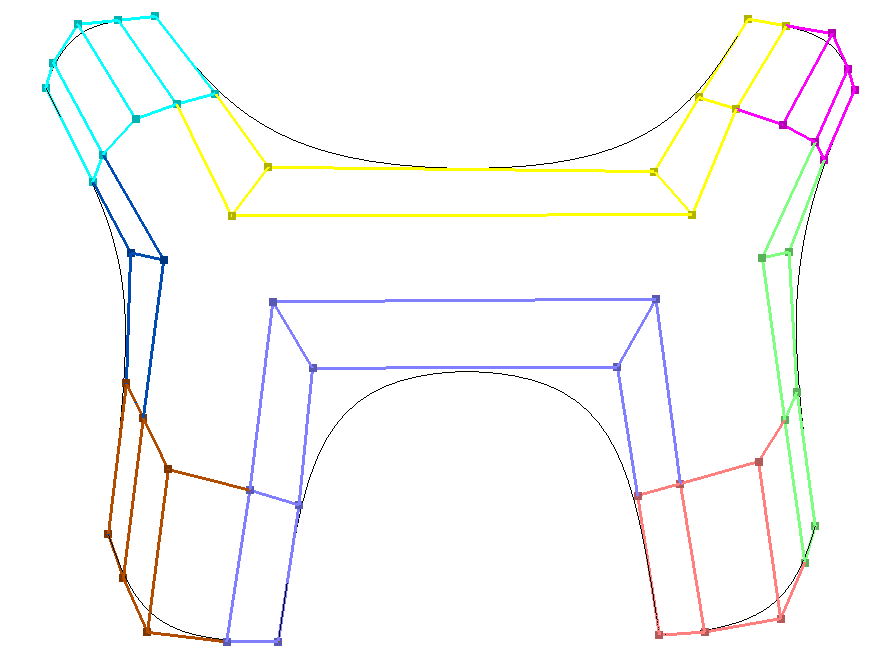
(a) Input ribbons

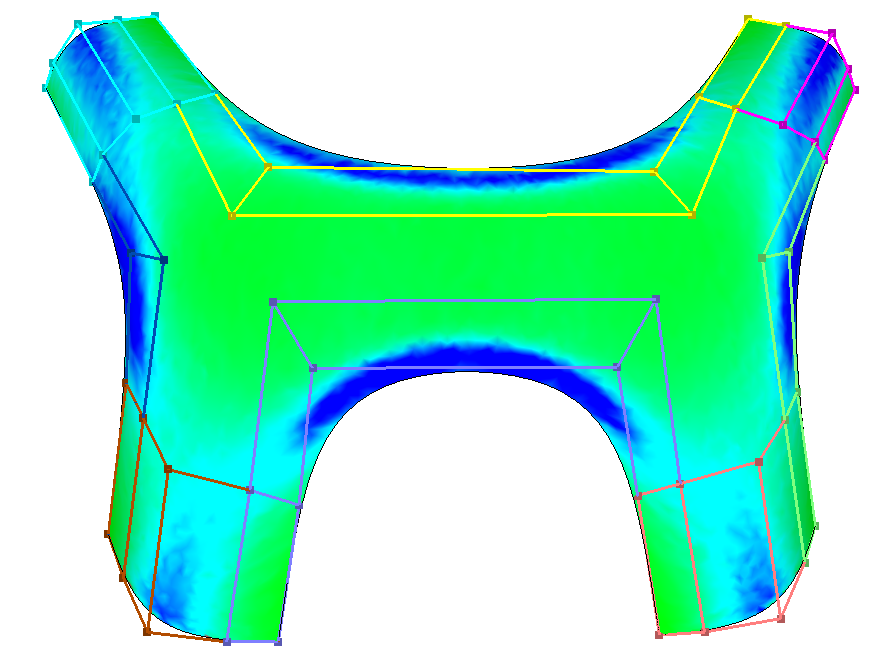
(b) GBS patch

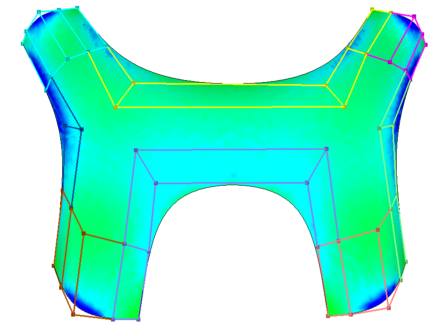
(c) Biharmonic patch

Figure 1: Comparison of vertex blend surfaces. Colors indicate mean curvature.

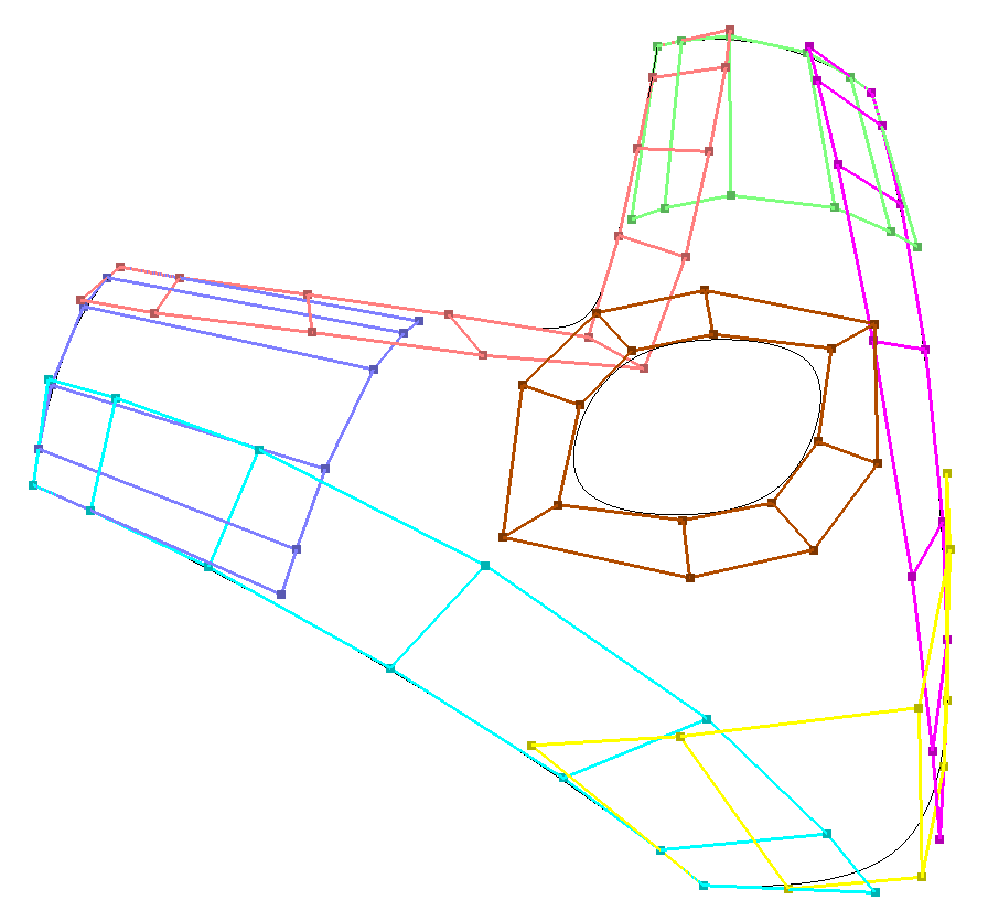
(a) Input ribbons

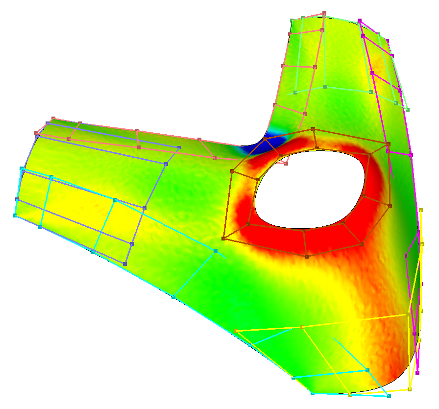
(b) GBS patch

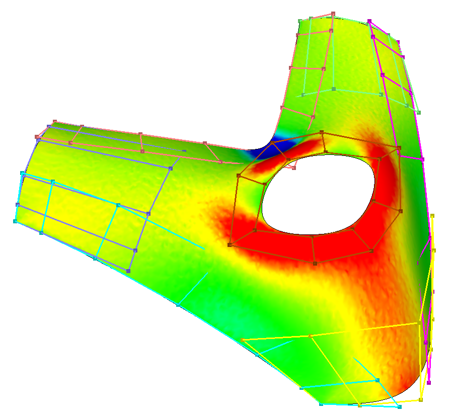
(c) Biharmonic patch

Figure 2: Comparison of multiply connected surfaces. Colors indicate mean curvature.

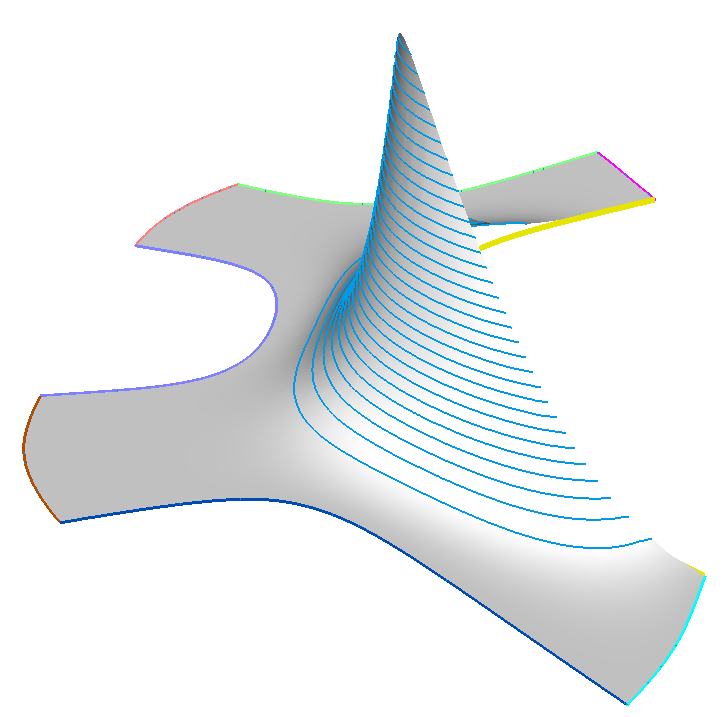
(a) GBS (boundary CP)

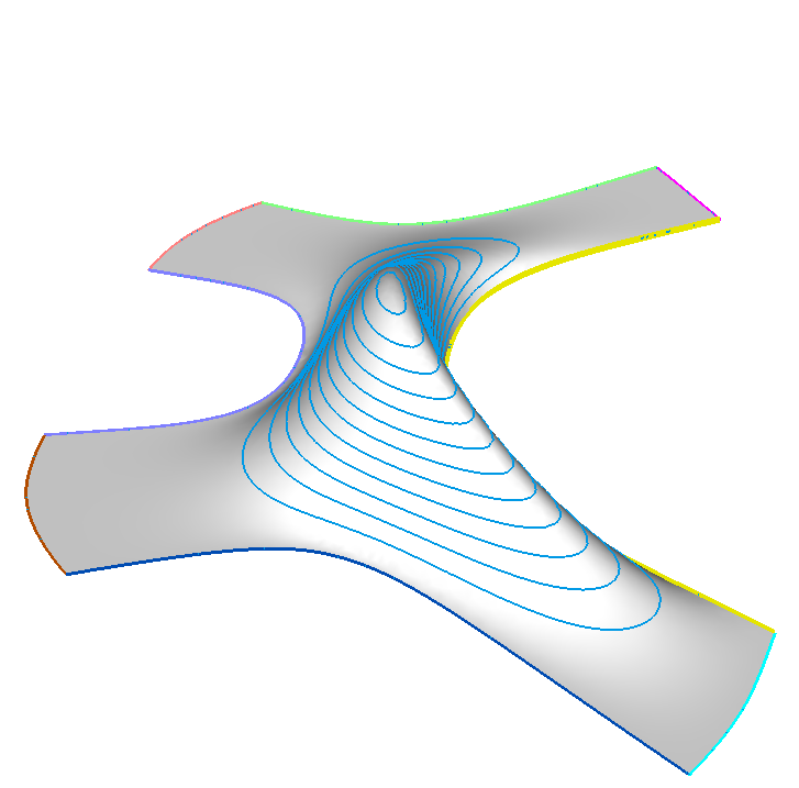
(b) GBS (tangent CP)

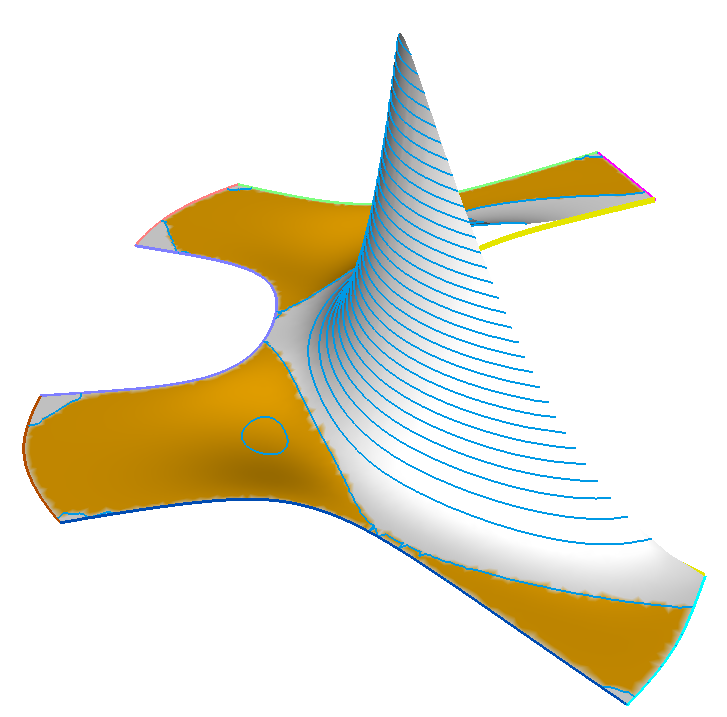
(c) Biharmonic (boundary CP)

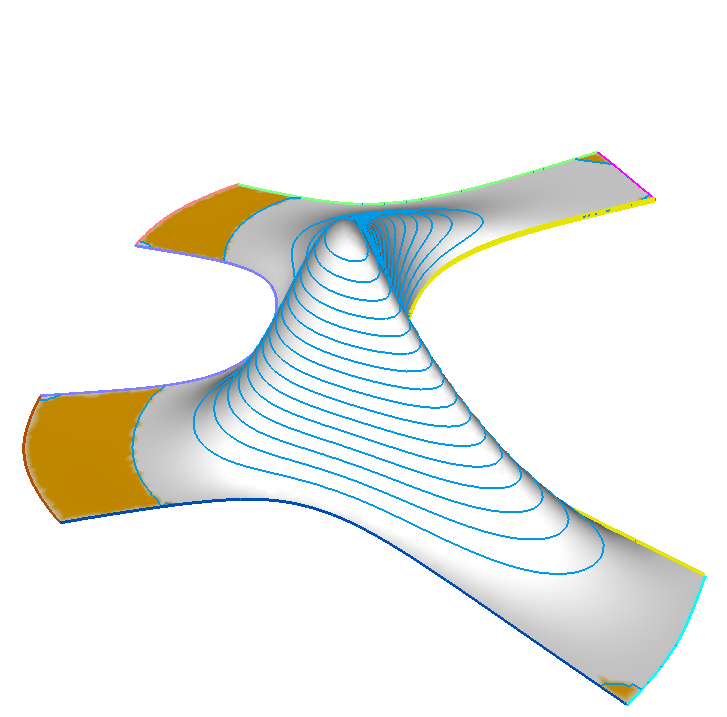
(d) Biharmonic (tangent CP)

Figure 3: Comparison of blend function level surfaces. Yellow color indicates negative values.

References

- (1) P. Kiciak, Geometric Continuity of Curves and Surfaces, Synthesis Lectures on Visual Computing, Morgan & Claypool Publishers (2017), 10.1007/978-3-031-02590-7.
- (2) J. Peters, Splines for meshes with irregularities, The SMAI Journal of computational mathematics 5 (2019) 161.
- (3) M. Vaitkus, T. Várady, P. Salvi and Á. Sipos, Multi-sided B-spline surfaces over curved, multi-connected domains, Computer Aided Geometric Design 89 (2021) 102019.
- (4) Á. Sipos, T. Várady, P. Salvi and M. Vaitkus, Multi-sided implicit surfacing with I-patches, Computers & Graphics 90 (2020) 29.
- (5) T. Várady, P. Salvi, M. Vaitkus and Á. Sipos, Multi-sided Bézier surfaces over curved, multi-connected domains, Computer Aided Geometric Design 78 (2020) 101828.
- (6) F. Martin and U. Reif, Trimmed spline surfaces with accurate boundary control, in Geometric Challenges in Isogeometric Analysis, vol. 49 of Springer INdAM Series, pp. 123–148, 2022, DOI.
- (7) M.A. Sabin, Transfinite surface interpolation, in The Mathematics of Surfaces VI, pp. 517–534, IMA, 1996.
- (8) C. Dyken and M.S. Floater, Transfinite mean value interpolation, Computer Aided Geometric Design 26 (2009) 117.
- (9) T. Várady, A. Rockwood and P. Salvi, Transfinite surface interpolation over irregular -sided domains, Computer-Aided Design 43 (2011) 1330.
- (10) P. Salvi, T. Várady and A. Rockwood, Ribbon-based transfinite surfaces, Computer Aided Geometric Design 31 (2014) 613.
- (11) T. Várady, Overlap patches: a new scheme for interpolating curve networks with -sided regions, Computer Aided Geometric Design 8 (1991) 7.
- (12) T. Várady, P. Salvi and G. Karikó, A multi-sided Bézier patch with a simple control structure, Computer Graphics Forum 35 (2016) 307.
- (13) G.J. Hettinga and J. Kosinka, Multisided generalisations of Gregory patches, Computer Aided Geometric Design 62 (2018) 166.
- (14) G.J. Hettinga and J. Kosinka, A multisided B-spline patch over extraordinary vertices in quadrilateral meshes, Computer-Aided Design 127 (2020) 102855.
- (15) H.P. Moreton and C.H. Séquin, Functional optimization for fair surface design, ACM SIGGRAPH Computer Graphics 26 (1992) 167.
- (16) R. Schneider and L. Kobbelt, Generating fair meshes with boundary conditions, in Geometric Modeling and Processing 2000, pp. 251–261, IEEE, 2000, DOI.
- (17) H. Pan, Y. Liu, A. Sheffer, N. Vining, C. Li and W. Wang, Flow aligned surfacing of curve networks, ACM Transactions on Graphics (TOG) 34 (2015) 127.
- (18) Y. Soliman, A. Chern, O. Diamanti, F. Knöppel, U. Pinkall and P. Schröder, Constrained Willmore surfaces, ACM Transactions on Graphics (TOG) 40 (2021) 112.
- (19) M. Botsch and L. Kobbelt, An intuitive framework for real-time freeform modeling, ACM Transactions on Graphics (TOG) 23 (2004) 630.
- (20) A. Jacobson, E. Tosun, O. Sorkine and D. Zorin, Mixed finite elements for variational surface modeling, Computer Graphics Forum 29 (2010) 1565.
- (21) J. Andrews, P. Joshi and N. Carr, A linear variational system for modelling from curves, Computer Graphics Forum 30 (2011) 1850.
- (22) M. Botsch and O. Sorkine, On linear variational surface deformation methods, IEEE Transactions on Visualization and Computer Graphics 14 (2007) 213.
- (23) O. Stein, E. Grinspun, M. Wardetzky and A. Jacobson, Natural boundary conditions for smoothing in geometry processing, ACM Transactions on Graphics (TOG) 37 (2018) 1.
- (24) O. Weber, R. Poranne and C. Gotsman, Biharmonic coordinates, Computer Graphics Forum 31 (2012) 2409.
- (25) R. Sawhney and K. Crane, Monte Carlo geometry processing: a grid-free approach to PDE-based methods on volumetric domains, ACM Transactions on Graphics (TOG) 39 (2020) 123.
- (26) P. Joshi, M. Meyer, T. DeRose, B. Green and T. Sanocki, Harmonic coordinates for character articulation, ACM Transactions on Graphics (TOG) 26 (2007) 71.
- (27) C. Mancinelli, M. Livesu and E. Puppo, A comparison of methods for gradient field estimation on simplicial meshes, Computers & Graphics 80 (2019) 37.
- (28) J. Peters, Smoothness, fairness and the need for better multi-sided patches, in Topics in Algebraic Geometry and Geometric Modeling, vol. 334 of Contemporary Mathematics, pp. 55–64, AMS, 2003, DOI.
- (29) J. Peters and K. Karčiauskas, An introduction to guided and polar surfacing, in 7th International Conference on Mathematical Methods for Curves and Surfaces, vol. 5862 of Lecture Notes in Computer Science, pp. 299–315, 2008, DOI.