Proposing an intelligent mesh smoothing method with graph neural networks

Abstract

In CFD, mesh smoothing methods are commonly utilized to refine the mesh quality to achieve high-precision numerical simulations. Specifically, optimization-based smoothing is used for high-quality mesh smoothing, but it incurs significant computational overhead. Pioneer works improve its smoothing efficiency by adopting supervised learning to learn smoothing methods from high-quality meshes. However, they pose difficulty in smoothing the mesh nodes with varying degrees and also need data augmentation to address the node input sequence problem. Additionally, the required labeled high-quality meshes further limit the applicability of the proposed method. In this paper, we present GMSNet, a lightweight neural network model for intelligent mesh smoothing. GMSNet adopts graph neural networks to extract features of the node’s neighbors and output the optimal node position. During smoothing, we also introduce a fault-tolerance mechanism to prevent GMSNet from generating negative volume elements. With a lightweight model, GMSNet can effectively smoothing mesh nodes with varying degrees and remain unaffected by the order of input data. A novel loss function, MetricLoss, is also developed to eliminate the need for high-quality meshes, which provides a stable and rapid convergence during training. We compare GMSNet with commonly used mesh smoothing methods on two-dimensional triangle meshes. The experimental results show that GMSNet achieves outstanding mesh smoothing performances with 5% model parameters of the previous model, and attains 8.62 times faster than optimization-based smoothing.

1 Introduction

With the rapid advancement of computer technology, computational fluid dynamics (CFD) has emerged as a crucial method for studying the principles of fluid dynamics. Its wide applications span diverse fields, including aerospace, hydraulic engineering, automotive engineering, and biomedicine [1, 2, 3, 4]. Normally, CFD simulations are performed by discretizing the governing physical equations and subsequently solving large-scale algebraic systems of discretized equations to obtain fluid variables. Discretization, a critical step in CFD, encompasses two key aspects: discretizing the governing physical equations and discretizing the computational domain [5]. The latter process, known as mesh generation, plays a fundamental role in CFD. It involves partitioning the computational domain into non-overlapping mesh elements, such as polygons in the two-dimensional region and polyhedra in the three-dimensional region [6]. The quality of the generated mesh profoundly impacts the convergence, accuracy, and efficiency of numerical simulations. Orthogonality, smoothness, distributivity and density distribution of mesh elements significantly influence the stability and convergence of the solution matrix [7]. Consequently, the quest for high-quality mesh generation remains a vibrant and active area in CFD research. During the practical mesh generation process, the initial generated mesh often fails to meet simulation requirements. To enhance the quality of the mesh, mesh quality improvement techniques are commonly employed, including mesh smoothing, face-swapping, edge-swapping, point insertion/deletion, and other techniques [8, 9, 10]. Among such techniques, mesh smoothing methods are the most commonly used approach to improve mesh quality.

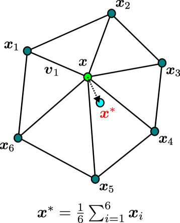
(a)

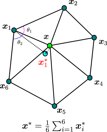
(b)

Figure 1: a) Laplacian smoothing. The StarPolygon of point $\boldsymbol{x}$ is formed by $\mathbf{S}(\boldsymbol{x})=\{\boldsymbol{x}_{1},\boldsymbol{x}_{2},\dots,\boldsymbol{x}_{6}\}$ as a hexagon. The optimized mesh nodes are then located at the arithmetic average of the coordinates of the nodes in the StarPolygon. b) Angle-Based smoothing. The figure shows the optimal position based on $\boldsymbol{x}_{1}$. This is achieved by rotating $\boldsymbol{x}$ to the angle bisector of the angle where $\boldsymbol{x}_{1}$ is located, resulting in $\boldsymbol{x}_{1}^{*}$. This process is repeated for other points in the mesh, and the final optimized points are obtained through arithmetic averaging.

Mesh smoothing can be categorized into two main types: heuristic smoothing and optimization-based smoothing [11]. One representative heuristic method is Laplacian smoothing [12] (shown in Figure 1a). In Laplacian smoothing, mesh node is placed at the arithmetic average of the coordinates of the nodes in the StarPolygon (a polyhedron containing the node, as shown in Figure 1) for smoothing. This method is efficient but may produce negative volume elements when the StarPolygon is non-convex. Angle-based smoothing achieves mesh smoothing by placing mesh node on the angle bisectors of the nodes of the StarPolygon (shown in Figure 1b) [13]. In addition to node-based methods, Centroidal Voronoi tessellation (CVT) smoothing [14] recalculates the Voronoi regions of each node through Lloyd iterations [15] and relocates the point to the centroid of the Voronoi region for smoothing. To enhance the efficiency of the Lloyd algorithm, deterministic methods have been proposed for calculating the new point location [16]. Although heuristic-based mesh smoothing methods are simple and efficient, their optimization capabilities are limited. They may lead to inverted elements, and the smoothness effect heavily relies on the design of heuristic functions. On the other hand, optimization-based methods achieve mesh smoothing by optimizing the mesh quality evaluation metric in the local area [17, 18, 19, 20]. Parthasarathy and Kodiyalam [17] formulate the mesh smoothing problem as a constrained optimization problem and utilize iterative optimization algorithms to optimize the mesh node positions. Despite the adoption of different mesh quality evaluation metrics and optimization methods in subsequent works, the optimization-based methods usually require solving optimization problems iteratively for mesh smoothing, resulting in low efficiency.

Recently, Artificial Intelligence (AI) methods have also been widely used in mesh-related fields. Most of these research works are devoted to applying AI methods to mesh quality evaluation [21, 22, 23], mesh density control [24, 25], mesh generation [26, 27, 28], mesh refinement [29, 30], mesh adapatation [31, 32, 33]. However, there is relatively little work on AI-based mesh smoothing. Guo et al. [11] firstly introduced a supervised learning approach to imitate optimization-based smoothing methods with feedforward neural networks. The proposed model, NN-Smoothing, improves the efficiency of optimization-based smothing by directly giving the optimal node position. However, feedforward neural networks suffer from fixed-dimensional inputs, necessitating separate models for mesh nodes with different degrees and data augmentation for different sequences of input nodes, thereby increasing the model’s training cost. Moreover, to train the model through supervised learning, high-quality mesh generation also incurs burdensome computational overhead.

To overcome such limitations, we present a novel mesh smoothing model, GMSNet, based on graph neural networks (GNNs) [34] in this paper. We propose a lightweight and efficient GNN model to learn the process of mesh smoothing. GMSNet avoids the overhead of solving the optimization problem by extracting features of the neighboring nodes of the mesh node to directly output better node position. We show that through the ability of graph neural networks to handle unstructured data, GMSNet can smooth nodes of varying degrees with a single model and elegantly solves the node input sequence problem without data augmentation. Once trained, it can be applied to smooth mesh with different shapes. We also propose a shift truncation operation to avoid introducing negative volume elements when smoothing the mesh. Beyond the proposed GMSNet, we introduce a novel loss function, MeticLoss, based on the mesh quality metrics to train the model, which further eliminates the overhead of generating high-quality meshes. We conduct extensive experiments among GMSNet and commonly used mesh smoothing algorithms on two-dimensional triangular meshes. The experimental results show that our model achieves a speedup of 8.62 times compared with optimization-based smoothing while achieving similar performance, and outstands all the other heuristic smoothing algorithms. The results also indicate that GMSNet can be applied to meshes that were unseen during training. Meanwhile, compared to previous NN-Smoothing model, GMSNet has only 5% of its model parameter, but obtains superior mesh smoothing performance. We also validate the effectiveness of proposed MetriLoss and shift truncation with comparative experiments. We summary our contributions as follows:

1. We propose a lightweight graph neural network model, GMSNet, for intelligent mesh smoothing. GMSNet can smoothing node with varying degrees and remain unaffected by the data input order. Additionally, we offer a fault-tolerance mechanism, shift truncation, to prevent GMSNet from generating negative volume elements

2. Basing on the mesh quality metrics, we introduce a novel loss function, MetricLoss, to train the model without necessity for high-quality meshes. MetricLoss exhibits a stable and rapid convergence during model training.

3. We validate the effectiveness of GMSNet through extensive experiments conducted on two-dimensional triangular meshes. The experimental results demonstrate that GMSNet achieves excellent mesh smoothing performance and significantly outperforms optimization-based smoothing with a average speedup of 8.62 times. Comparative experiments are also conducted to showcase the effectiveness of the proposed MetricLoss and shift truncation operation.

The remaining parts of this paper are organized as follows. In Section 2, we introduce commonly used mesh smoothing methods and applications of neural networks in the field of mesh. In Section 3, we present the proposed model, providing detailed explanations of the mesh data preprocessing, design of the model’s architecture, loss function and training method. In Section 4, we conduct experiments to compare the performance of our proposed model with baseline models and discuss the effectiveness of loss function and shift truncation. Finally, in the conclusion section, we summarize the entire paper and propose potential future work that can be explored.

2 Realted work

2.1 Heuristic mesh smoothing

Laplacian smoothing is the most commonly used heuristic mesh smoothing method. It updates the node coordinate to the arithmetic average of nodes in StarPolygon. Weighted Laplacian smoothing [35] introduces additional weights or importance factors to the neighboring nodes or edges during the smoothing process, offering more control over the smoothing effect and preserving specific features of the mesh. Smart Laplacian smoothing [18] includes a check before each node movement to assess whether the operation will improve the mesh quality. If the mesh quality does not improve, the movement of the mesh node is skipped, resulting in a more efficient process. Angle-based mesh smoothing achieves smoothness by considering the angles of the mesh nodes. In this method, the node is rotated to align with the angle bisectors of each node in StarPolygon. Since the angle bisectors of the various nodes of the StarPolygon may not coincide, the final node positions require additional calculation. This can be achieved by calculating the average of the node coordinates or by solving a least squares problem. CVT smoothing positions the node at the centroids of the Voronoi region defined by the mesh node. To enhance the efficiency of the Lloyd algorithm in the solving process, more efficient method has been designed to calculate the centroids, as described below:

$$\boldsymbol{x}_{i}^{*}=\frac{1}{\left|\Omega_{i}\right|}\sum_{T_{j}\in\Omega_{i}}\left|T_{j}\right|C_{j}$$ (1)

where $\boldsymbol{x}_{i}^{*}$ represents the new node position, $|\Omega_{i}|$ is the total area of the node’s StarPolygon, $|{T_{j}}|$ is the area of the $j$ th triangle, and $C_{j}$ is the circumcenter of the $j$ th triangle.

It is worth noting that there is no absolute boundary between heuristic smoothing and optimization-based smoothing. From another perspective, heuristic mesh smoothing can also be viewed as an optimization-based approach. For instance, Laplacian smoothing can be viewed as minimizing the energy function $E=\frac{K}{2}\sum_{i=1}^{K}\left|\boldsymbol{v}_{i}\right|^{2}$, where $\boldsymbol{v}_{i}$ represents the edge from $\boldsymbol{x}$ to $\boldsymbol{x}_{i}$, and $K$ is the number of nodes in the StarPolygon (shown in Figure 1a). Similarly, Angle-based mesh smoothing can be seen as minimizing the energy function $E=\frac{K}{2}\sum_{i=1}^{2K}\theta_{i}^{2}$, where $\theta_{i}$ is the angle between the edge from $\boldsymbol{x}$ to $\boldsymbol{x}_{i}$ and the edge of the polygon (shown in Figure 1b). The primary advantage of heuristic mesh smoothing lies in its efficiency. However, its smoothing performance often is inferior to that of optimization-based smoothing. Furthermore, the effectiveness of heuristic mesh smoothing heavily relies on the design of the heuristic functions.

2.2 Optimization-based smoothing

The mesh smoothing method based on optimization can be formalized as the following problem: Given an initial mesh with node positions $\boldsymbol{x}_{i}$ and a set of constraints and the objective function $f$, the goal is to find a new node positions $\boldsymbol{x}_{i}^{*}$ that minimizes the objective function $f$. Mathematically, this can be expressed as:

$$\boldsymbol{x}_{i}^{*}=\underset{\boldsymbol{x}_{i}}{\arg\min}f\left(\boldsymbol{x}_{i},\mathbf{S}\left(\boldsymbol{x}_{i}\right)\right)$$ (2)

$$\text{s.t.}\quad\boldsymbol{x}_{i}\in\mathcal{X}$$

where $\boldsymbol{x}_{i}^{*}$ represents the new position of the mesh node $\boldsymbol{x}_{i}$, $f$ is some mesh quality evaluation function, $\mathcal{X}$ is the feasible set satisfying constraints on $\boldsymbol{x}_{i}^{*}$, and $\mathbf{S}(\boldsymbol{x}_{i})$ is the set of nodes of the StarPolygon of $\boldsymbol{x}_{i}$. It is important to mention that the input of this function also includes the connectivity between nodes, which is omitted here for clarity. Different choices of evaluation functions lead to different mesh smoothing methods, reflecting our emphasis on different mesh qualities. Commonly used evaluation functions include the maximum minimum angle [36], respect ratio, and distort ratio, among others [17]. If the function $f$ is differentiable, the optimal point of this constrained optimization problem may be solved by setting the gradient $\nabla f=0$ to obtain an explicit expression. However, in most cases, it is difficult to derive explicit expressions for $\boldsymbol{x}_{i}^{*}$ as in Laplacian smoothing and Angle-based smoothing. Iterative methods are often used to solve $\boldsymbol{x}_{i}^{*}$, which are of low efficiency. Therefore, developing an efficient way to solve the optimal positions is a problem that needs to be addressed.

2.3 Neural networks in mesh-related fields

Inspired by the neurons in the human brain, artificial neural networks are utilized to learn complex function mappings. They find extensive applications in machine learning and artificial intelligence, addressing tasks like image recognition, speech recognition, natural language processing, and more [37, 38, 39, 40]. Recently, neural networks have found significant application in various domains related to meshes. In the realm of mesh quality evaluation, GridNet, a convolutional neural network model, was introduced by Chen et al. [21], along with the NACA-Market dataset, to facilitate automated evaluation of structured mesh quality. Extending this notion to unstructured meshes, Wang et al. [22] employed graph neural networks for mesh quality assessment. In the pursuit of refining mesh distribution, Zhang et al. [24] employed an artificial neural network to enhance conventional mesh generation software, enabling prediction of local mesh density throughout the domain. This approach was further expanded to tetrahedral meshes, as demonstrated convincingly through extensive testing [25]. In the domain of intelligent mesh generation, Daroya et al. [26] presented an algorithm that leverages global structural information from point clouds to achieve high-quality mesh reconstruction. Similarly, Papagiannopoulos et al. [27] harnessed data extracted from meshed contours to train neural networks, enabling accurate approximation of the number, placement, and interconnectivity of nodes within the meshing domain. Taking a novel differential approach, Chen et al. [28] introduced MGNet, an unsupervised neural network methodology for generating structured meshes, yielding promising results. Beyond generation, artificial intelligence techniques have also made significant contributions to mesh refinement and adaptation. Bohn and Feischl [29] employed recurrent neural networks to learn optimal mesh refinement algorithms, establishing its prowess as an effective black-box tool for enhancing a wide spectrum of partial differential equations. Enriching variational mesh adaptation, Tingfan et al. [31] seamlessly integrated a machine learning regression model to expedite flow field estimation on updated meshes. Meanwhile, Wallwork et al. [32] devised a data-driven goal-oriented mesh adaptation strategy, underpinned by a trained neural network, effectively supplanting the computationally expensive error estimation phase in the adaptation process. Furthermore, Fidkowski and Chen [33] ingeniously employed Artificial Neural Networks to ascertain optimal anisotropy in computational meshes, yielding enhanced mesh efficiency in comparison to conventional methods. In term of mesh smoothing, NN-Smoothing [11] imitates optimization-based mesh smoothing using feedforward neural networks, significantly enhancing the efficiency of optimization-based mesh smoothing. However, separate models training and expensive high-quality mesh generation incur significant computational overhead.

In addition to conventional deep learning algorithms, graph neural networks [34] were introduced to enhance the learning capacity of artificial intelligence methods for handling non-structured data. GNNs utilize graph convolutions [41] to incorporate the topological connections in the feature learning process on graphs. As meshes can be naturally represented as graph data, GNNs have found extensive applications in various computational fluid dynamics fields, including mesh refinement, flow field simulation, turbulence modeling, and more [42, 43, 44, 45, 46]. Therefore, we argue that applying GNNs to mesh smoothing is a promising and effective solution.

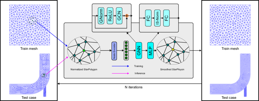
Figure 2: The architecture of GMSNet. GMSNet smoothes the mesh by calculating the optimized position for each mesh node. The process begins with the normalization of the input StarPolygon. Next, feature transformation is performed on the normalized features, and information from the StarPolygon nodes is integrated using graph convolution. Finally, the model predicts the optimized node positions through fully connected (FC) layers. In the figure, GNorm represents the GraphNorm operation, and IS-Norm represents the InstanceNorm operation. The model iterates $N$ times over the entire mesh to perform the smoothing operation. After training, GMSNet can be applied to previously unseen meshes, such as the pipe’s mesh.

3 Methodology

3.1 Problem formulation

The mesh smoothing problem involves enhancing the quality of a mesh by adjusting the positions of its nodes while maintaining the connectivity between them. Mesh smoothing processes are defined as functions that operate on the mesh, taking the mesh nodes and their connections as inputs and providing new coordinates for the mesh nodes as outputs. For each mesh node, the input of the smoothing function is itself and its StarPolygon, which comprises the node’s one-ring neighbors. In this paper, we define the mesh as a node graph. Specifically, given a node $\boldsymbol{x}_{0}$ and its StarPolygon, we represent it with a graph $\mathcal{G}=(\mathcal{V},\mathcal{E})$, where $\mathcal{V}=\{\boldsymbol{x}_{0},\boldsymbol{x}_{1},\boldsymbol{x}_{2},\dots,\boldsymbol{x}_{n}\}$ represents the node and nodes in the StarPolygon, $\boldsymbol{x}_{i}$ is the coordinate of node $i$ in StarPolygon, $n$ is the number of nodes in the StarPolygon, and $\mathcal{E}=\{(i,j)\mid\text{if }\boldsymbol{x}_{i}\text{ is connected with }\boldsymbol{x}_{j}\}$ represents the connections between the nodes. A typical smoothing process is iterative, where at the $t$ th iteration step, the initial node graph is denoted as $\mathcal{G}_{t}$, and the optimized node position for the center node can be represented as:

$$\boldsymbol{x}_{0}^{t+1}=\mathcal{F}(\mathcal{G}_{t})=\mathcal{F}(\mathcal{V}_{t},\mathcal{E})$$ (3)

In this paper, we employ graph neural networks to learn the function $\mathcal{F}$ for mesh smoothing.

3.2 GMSNet

3.2.1 Lightweight model design

The mesh smoothing model based on graph neural networks is depicted in Figure 2. Given a graph consisting of mesh nodes and edges, our goal is to compute a more optimal mesh node position for each mesh node to smoothing the mesh. In the model, we use the coordinate positions as node features, denoted as $X\in\mathbb{R}^{(n+1)\times 2}$ ($n$ nodes in the StarPolygon and one free node to move). The connectivity between nodes is represented by the adjacency matrix $A\in\mathbb{R}^{(n+1)\times(n+1)}$ (node index $i$ is omitted for clarity).

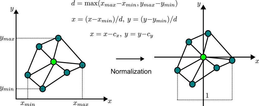
Figure 3: Data normalization. The StarPolygon to be processed is normalized to the center of the coordinate axis. In the figure, $d$ represents the maximum size of the StarPolygon, $x$ and $y$ represent the coordinates to be scaled, and $c_{x}$ and $c_{y}$ are the normalized coordinates of the target node after the scaling.

To ensure the model’s scale invariance, we apply node normalization during processing. The model normalizes the node input using min-max normalization on $X$, restricting it to the range of 0 and 1, and subsequently performs a translation to center the node around the coordinate origin. After model processing, we employ an affine transformation to map the node positions back to their original scale. Data normalization is illustrated in Figure 3. After normalizing the data, we transform the features by a linear layer, which can be expressed as

$$X_{h}=\mathrm{Norm}(X)\mathbf{W}_{l}+\mathbf{b}_{l}$$ (4)

where $\mathrm{Norm}$ represents the normalization operation, $\mathbf{W}_{l}\in\mathbb{R}^{2\times H}$ and $\mathbf{b}_{l}$ is the transformation matrix and bias of the linear layer, $H$ is the dimension of the hidden feature, and $X_{h}\in\mathbb{R}^{(n+1)\times H}$ is the output of the linear layer. Subsequently, we employ a residual graph convolutional network (GCN) layer [41, 47] to compute the features of the hidden layer based on the features of the nodes in the StarPolygon. The process involves normalizing the features outputted by the linear layer using GraphNorm [48], followed by an activation layer, a convolutional layer, and a summation layer to calculate the hidden features of the nodes. This process can be represented as:

$$\hat{X}_{h} =\mathrm{GraphNorm}(X_{h})$$ (5)

$$X_{g} =\mathrm{GCN}(\mathrm{ReLU}(\hat{X}_{h}),\tilde{A})+\hat{X}_{h}$$ (6)

$$=\tilde{A}[\mathrm{ReLU}(\hat{X}_{h})]\mathbf{W}_{g}+\hat{X}_{h}$$ (7)

where $\tilde{A}$ is the normalized adjacency matrix, ReLU is activation function, $\mathbf{W}_{g}$ is the parameter of GCN layer, and $X_{g}$ represents the final features output by the residual GCN layer. The final position of the center node is obtained through a two-layer fully connected neural network with InstanceNorm [49]. Let $i_{c}$ be the index of the center node, then the optimized node position is given by:

$$\boldsymbol{x}^{*}=\mathrm{MLP}(X_{g})[i_{c}]$$ (8)

The smoothing algorithm should possess the capability to handle nodes with varying degrees and remain unaffected by the order of node inputs. In the NN-Smoothing model, handling nodes with different degrees is achieved by training separate models, while the order of node inputs is addressed through data augmentation by varying the starting node in the ring of StarPolygon. However, due to the permutation invariance property of graph neural network models, where the output remains unchanged despite permutations in the input order (such as in the sum function or mean function), GMSNet can effectively handle nodes with different degrees without the need for training separate models or performing data augmentation.

Table 1: Comparison among optimization-based smoothing, NN-Smoothing and GMSNet

Method	Speed	Labeled high-quality mesh	Varying node degrees	Node input order
OptimSmoothing1	Slow	Not acquiring	Not affected	Not affected
NN-Smoothing	Fast	Acquiring	Training separate models	Data augmentation
GMSNet	Fast	Not acquiring	Not affected	Not affected

• Optimization-based smoothing.

3.2.2 Model training

In the NN-Smoothing method, the model is trained using supervised learning, and the labeled high-quality meshes are generated using optimization-based smoothing, which is a time-consuming task. In contrast, the proposed GMSNet directly learns the optimization process for mesh smoothing. This process can be illustrated by comparing it with optimization-based smoothing. In optimization-based smoothing, taking gradient descent as the optimization method and given a mesh quality function $f$ to be optimized, the objective is to find its minimum value. In the $k$ th iteration, the optimization algorithm updates the position as $\boldsymbol{x}_{k+1}=\boldsymbol{x}_{k}-\alpha\nabla_{\boldsymbol{x}}f(\boldsymbol{x}_{k},\mathbf{S}(\boldsymbol{x}_{0}))$, where $\nabla_{\boldsymbol{x}}f(\boldsymbol{x}_{k},\mathbf{S}(\boldsymbol{x}_{0}))$ is the gradient of $f$ and $\alpha$ is the step size. By iteratively updating $\boldsymbol{x}_{k}$, the function converges to a local or global optimum $\boldsymbol{x}^{*}$. In contrast, NN-Smoothing directly predicts the optimal point for mesh smoothing, i.e., $\boldsymbol{\hat{x}}^{*}=\mathrm{NN}(\boldsymbol{x}_{0},\mathbf{S}(\boldsymbol{x}_{0}))$. However, this approach requires labeled high-quality meshes generated through the optimization algorithm, which is time-consuming. On the other hand, the GMSNet model does not require labeled data to learn the smoothing process for mesh nodes. Instead, the training process is driven by the quality evaluation metric of the mesh elements, which can be expressed as:

$$\mathbf{W}^{*} ={\arg\min}_{\mathbf{W}}\mathcal{L}(\boldsymbol{\hat{x}}^{*},\mathbf{S}(\boldsymbol{x}_{0}))$$ (9)

$$={\arg\min}_{\mathbf{W}}\mathcal{L}(\mathcal{F}_{\mathbf{W}}(\boldsymbol{x}_{0},\mathbf{S}(\boldsymbol{x}_{0})),\mathbf{S}(\boldsymbol{x}_{0}))$$

where $\mathcal{L}$ is the loss function constructed using a mesh quality metric, $\mathcal{F}_{\mathbf{W}}$ is learned through the proposed model, and ${\mathbf{W}}$ is the parameters of the model. The loss function is based on the mesh element evaluation metric, and the model optimizes the positions of mesh nodes by minimizing this function.

The main distinction between this approach and NN-Smoothing lies in the training data. In the proposed method, there are no high-quality meshes provided for the labels. Instead, the learning process relies solely on minimizing the mesh quality metric function. The primary divergence from optimization-based mesh smoothing methods is that this approach directly offers optimized positions for mesh nodes without the need to solve an optimization problem, resulting in a significant improvement in the efficiency of mesh smoothing. A comprehensive comparison of the three aforementioned methods is shown in Table 1.

3.2.3 MetricLoss

There are several metrics available to evaluate the quality of mesh elements, including the maximum angle, minimum angle, Jacobian matrix, aspect ratio, and others. In our case, we adopt the aspect ratio $q=\frac{{m^{2}+n^{2}+l^{2}}}{{4\sqrt{3}S}}$ to assess the mesh quality, where $m$, $n$, $l$ are the edges of the triangle, and $S$ is the area of the triangle. For an equilateral triangle, this value is 1, while for a degenerate triangle, it approaches $+\infty$. However, the range of this metric is too large, which can cause gradient explosion, especially for poor-shape elements. To address this issue, we use $1-\frac{1}{q}$ as the evaluation metric for mesh elements. For equilateral triangles, this value is 0, while for degenerate triangles, it is 1. The formal definition of the loss function is as follows:

$$\mathcal{L}(\boldsymbol{x},\mathbf{S}(\boldsymbol{x})) =\frac{1}{|\mathbf{S}(\boldsymbol{x})|}\sum_{i=1}^{|\mathbf{S}(\boldsymbol{x})|}{(1-\frac{1}{q_{i}})}$$ (10)

$$=\frac{1}{|\mathbf{S}(\boldsymbol{x})|}\sum_{i=1}^{|\mathbf{S}(\boldsymbol{x})|}{(1-\frac{4\sqrt{3}S_{i}}{m_{i}^{2}+n_{i}^{2}+l_{i}^{2}})}$$

where $|\mathbf{S}(\boldsymbol{x})|$ is the number of nodes in the StarPolygon, $m_{i}$,$n_{i}$,$l_{i}$ are the edges of triangle $T_{i}$, and $q_{i}$ is the quality of $T_{i}$. We validated the effectiveness of our designed loss function in Section 4.4.

3.2.4 Shift truncation

In the process of mesh generation and mesh smoothing, it is important to ensure that the generated mesh avoids negative volume elements. However, mesh smoothing algorithms can sometimes lead to the generation of negative volume elements, as depicted in Figure 4. For instance, in the case of Laplacian smoothing, when dealing with non-convex StarPolygons, negative volume elements may arise (as illustrated in Figure 4a). Similarly, during CVT smoothing, the calculation of the Voronoi centroid for elongated mesh elements can result in shifts that extend far away from the StarPolygon region, as shown in Figure 4b (in the case of degenerate mesh elements, the centroid position may even be at an infinite distance). Additionally, in optimization algorithms, using a uniform step size for different scales of mesh elements can also lead to the production of negative volume elements, as the optimization process may overshoot the optimal position.

(a)

(b)

(c)

Figure 4: a) For non-convex StarPolygons, Laplace smoothing may move nodes outside the StarPolygon. b) Computing the circumcenter of triangles is necessary for CVT smoothing. For highly distorted mesh element, it circumcenter is far away from the StarPolygon, resulting in negative volume elements. b) Shift truncation. In the training and inference phases of the model, we truncate the shift to avoid generating negative volume elements.

Negative volume elements can also occur during the training and inference stage of neural network-based smoothing algorithms. The generation of negative volume elements does not disrupt the learning process, as verified in Section 4.3. With the model training, the occurrence of negative volume elements gradually decreases. However, due to the uncertainty of neural networks, although rare, it is still possible for the model to introduce negative volume elements during the inference stage. Hence, a method is required to prevent the occurrence of negative volume elements. The simplest approach is to set the displacements that result in negative volume elements to zero. However, this approach hinders the update of poorly shaped mesh elements, which is precisely the optimization goal of mesh smoothing. Therefore, we have adopted a line search method to handle negative volume elements, as depicted in Figure 4c. We repeatedly half the shift which introduces the negative volume elements until no negative volume element is generated. We investigate the effect of shift truncation on the model in Section 4.3.

4 Experiments

4.1 Exprimental Setup

(a) Train data

(b) Supervised data

Figure 5: Mesh examples of the dataset for NN-Smoothing and GMSNet training. Supervised data is not utilized during the training of GMSNet.

In this section, we conducted a comprehensive performance comparison of the proposed GMSNet with five baseline smoothing methods (algorithms). The baseline methods we evaluated are as follows: Laplacian smoothing [18], Angle-based smoothing [13], CVT smoothing [14], Optimization-based smoothing, and NN-Smoothing [11]. Below are the implementation details for each baseline model:

• All models adopted the asynchronous updating, where the mesh nodes are directly updated after each optimization step (as opposed to computing the updates for all nodes and then updating them together).

• Smart Laplacian smoothing was adopted to prevent negative volume elements.

• In the Angle-based smoothing, the final node positions were obtained by averaging the optimized positions computed for each angle in the StarPolygon.

• The CVT smoothing employed the Equation 1 to improve the algorithm’s performance.

• The Optimization-based smoothing used MetricLoss defined in section 3.2.3 as the objective function and employed Adam [50] as the optimizer. Each node was optimized for a maximum of 20 iterations.

• The NN-Smoothing followed the implementation approach in the original paper. For nodes with different degrees, we trained different models to smooth the meshes. Additionally, Laplacian smoothing was used to handle nodes with degrees other than 3, 4, 5, 6, 7, 8, and 9.

We trained the model using two-dimensional triangle meshes, comprising a total of 20 meshes. The dataset was split into training, validation, and testing sets in a ratio of 6:2:2. Each mesh has distinct sizes and densities, randomly generated before the training. The mesh nodes are positioned randomly within the geometric domain, and the meshes are generated using Delaunay triangulation [51]. Example of the meshes is showns in Figure 5a.

In the experiment, we utilized the final optimization results obtained from the Optimization-based smoothing as the training labels for the NN-Smoothing model, which is shown in Figure 5b. Simultaneously, we trained the GMSNet without incorporating labels during the training process using the same dataset. For both neural network models, we employed Adam [50] as the optimizer with an initial learning rate of 1e-2. Throughout the training process, the learning rate was dynamically adjusted based on the performance on the validation set. In each training epoch, we randomly sampled 32 mesh nodes from each mesh to train the models. Despite training with only a partial sampling of mesh nodes, the models converge effectively.

4.2 Experimental results

We conducted tests on four mesh cases to evaluate the model’s smoothing performance. To test the performance of the model more thoroughly, we constructed meshes containing highly distorted elements as test cases, as shown in the first column of Figure 7. For the first two meshes, mesh nodes were generated by uniform sampling within the geometric domain. The latter two meshes were initially created using meshing software to generate high-quality meshes, and then manual adjustments were made to introduce distorted mesh elements.

To facilitate a fair comparison among different models, we have implemented the algorithms within the same framework. The variations among the algorithms lie in how they generate the optimized point positions. It is essential to mention that we have employed serial algorithms in our study. However, for simpler algorithms like Laplacian smoothing, updating all nodes simultaneously is straightforward and fast. We have chosen the minimum angle, maximum angle, and the reciprocal of the aspect ratio as evaluation metrics for mesh quality. We conducted ten experimental runs for each case, with a maximum of 100 smoothing iterations per experiment. The best-smoothed mesh was selected as the final result based on the weighted quality metric, which is defined as:

$$\hat{q} =\frac{1}{6}[\frac{\alpha_{\text{mean}}+\alpha_{\text{min}}+120-\beta_{\text{max}}-\beta_{\text{mean}}}{60}$$ (11)

$$+\left(\frac{1}{q}\right)_{\text{mean}}+\left(\frac{1}{q}\right)_{\text{min}}]$$

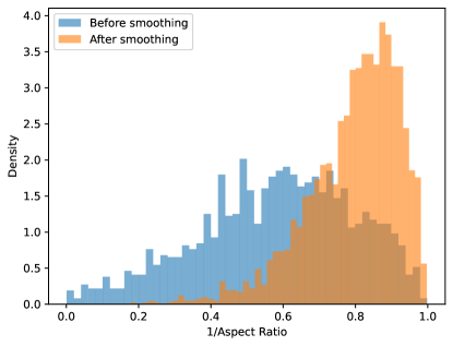
(a) Sqaure mesh

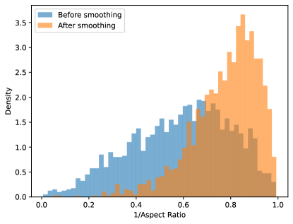
(b) Circle mesh

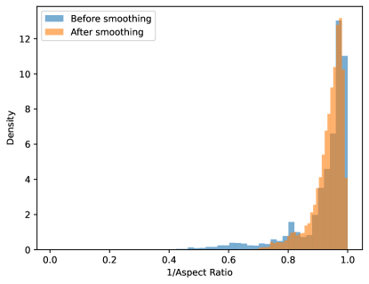
(c) Airfoil mesh

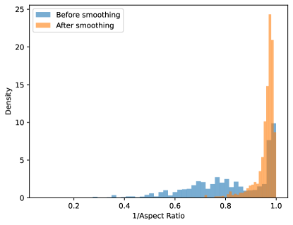
(d) Pipe mesh

Figure 6: The quality distribution of mesh elements before and after GMSNet smoothing.

where $\alpha$ is minimum angle, $\beta$ is the maximum angle, and $q$ is the aspect ratio. Furthermore, the algorithm speed is measured in terms of the time taken to process a single mesh node. The results of mesh smoothing using the GMSNet are depicted in the second column of Figure 7, and a comprehensive comparison of the performances of each algorithm is summarized in Table 2.

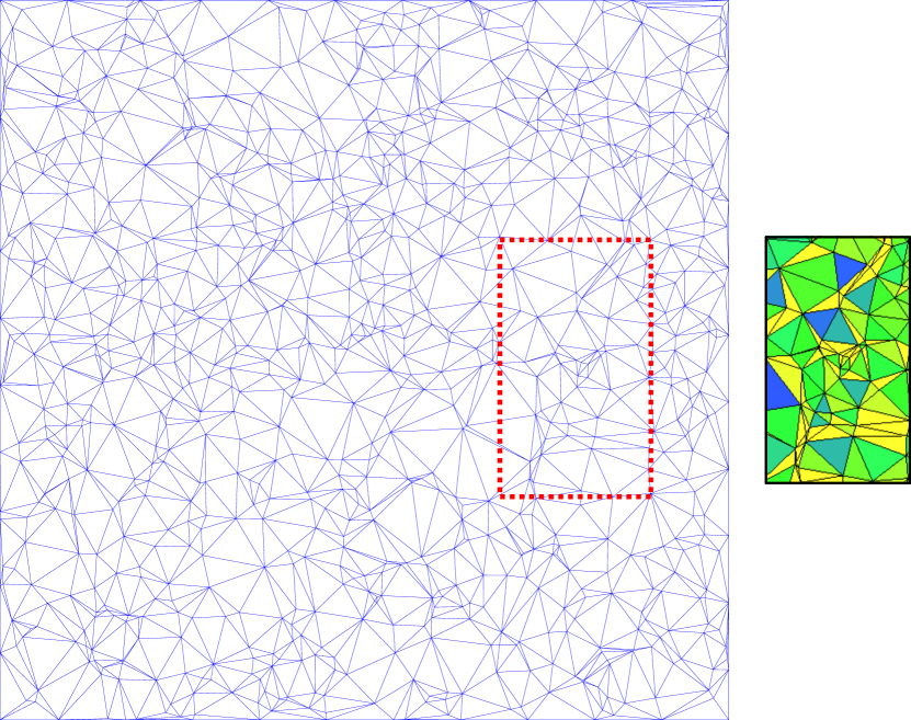
(a) Square mesh before smoothing

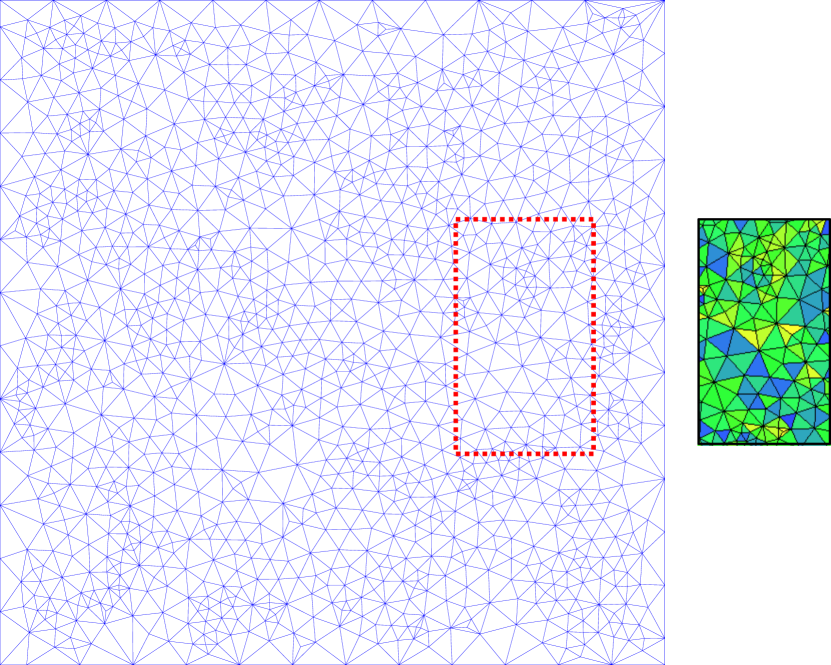
(b) Square mesh after smoothing

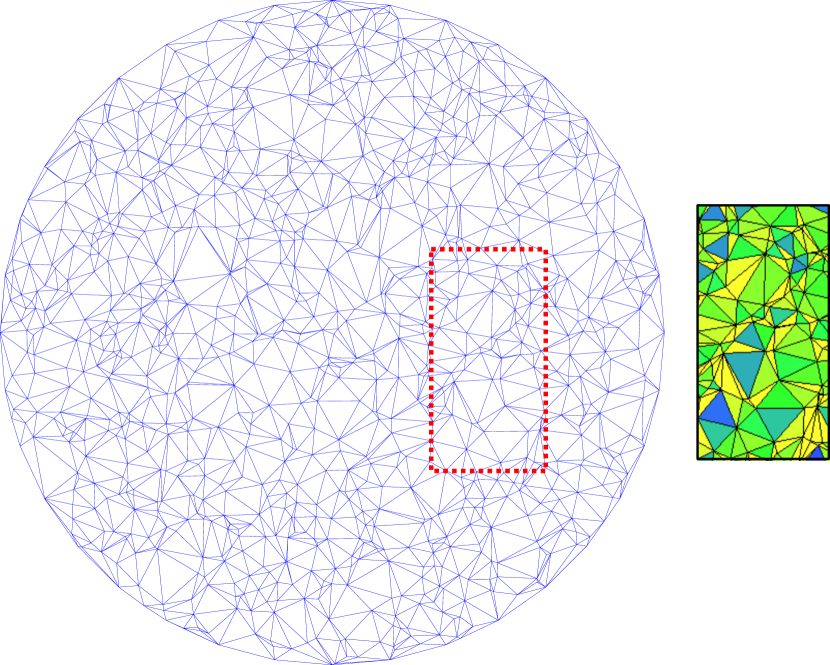
(c) Circle mesh before smoothing

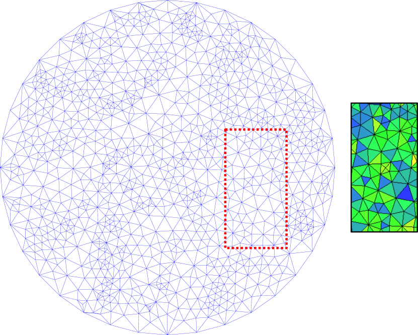
(d) Circle mesh after smoothing

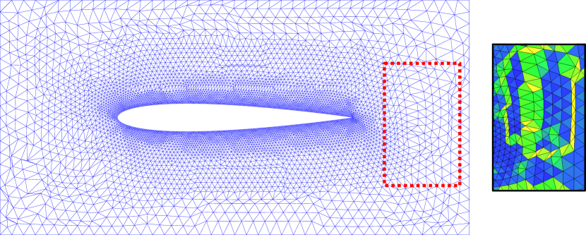
(e) Airfoil mesh before smoothing

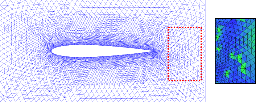
(f) Airfoil mesh after smoothing

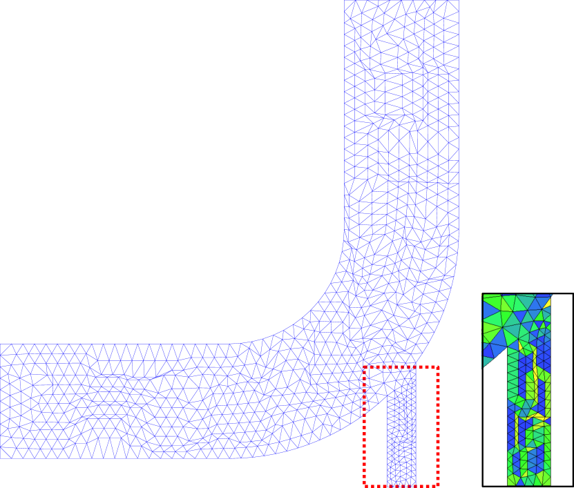
(g) Pipe mesh before smoothing

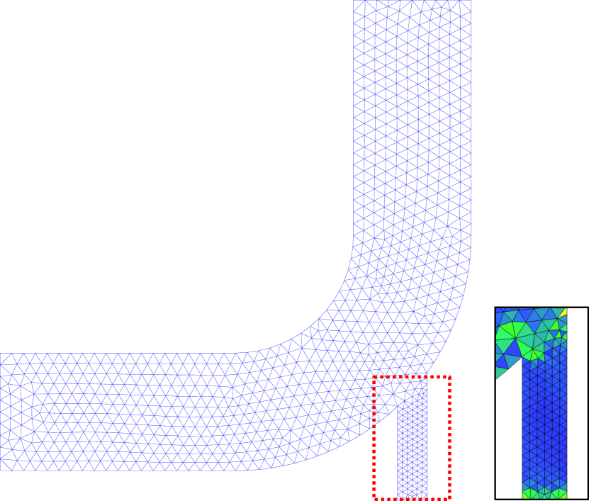
(h) Pipe mesh after smoothing

Figure 7: Mesh smoothing results of GMSNet on the test cases. Mesh nodes in meshes a) and c) are randomly generated in the domain, and mesh nodes in meshes e) and g) are manually adjusted to introduce distorted elements. High-quality elements are colored blue, and low-quality elements are colored yellow.

Table 2: Performance of mesh smoothing algorithms

		Min. Angle		Max. Angle		$\frac{1}{\text{Aspect ratio}}$		s/per node
Mesh	Algorithm	min	mean	max	mean	min	mean
Square	Origin	0.04	29.65	179.82	95.09	0.00	0.58	-
	LaplacianSmoothing	12.38	43.97	147.67	79.44	0.25	0.79	1.26E-03
	AngleSmoothing	10.52	41.26	148.6	81.76	0.22	0.76	2.36E-03
	CVTSmoothing	2.55	40.88	170.6	84.04	0.05	0.75	4.60E-03
	OptimSmoothing	16.33	43.94	136.99	80.7	0.32	0.79	2.29E-02
	NN-Smoothing	9.14	43.58	158.97	79.79	0.16	0.79	1.97E-03
	GMSNet	13.99	43.81	151.39	79.81	0.22	0.79	2.58E-03
Circle	Origin	0.29	30.38	179.05	94.60	0.01	0.59	-
	LaplacianSmoothing	1.43	42.86	174.53	81.19	0.03	0.78	1.21E-03
	AngleSmoothing	1.95	39.47	173.97	84.23	0.04	0.73	2.30E-03
	CVTSmoothing	3.19	39.98	172.98	85.59	0.05	0.73	4.35E-03
	OptimSmoothing	6.52	43.31	154.66	81.9	0.15	0.78	2.32E-02
	NN-Smoothing	1.26	41.1	176.04	83.86	0.03	0.75	1.88E-03
	GMSNet	2.2	43	169.21	81.29	0.05	0.78	2.38E-03
Airfoil	Origin	0.25	53.25	178.91	67.84	0.01	0.92	-
	LaplacianSmoothing	26.36	54.91	111.02	65.78	0.51	0.94	1.30E-03
	AngleSmoothing	20.26	53.49	118.76	66.64	0.42	0.93	2.54E-03
	CVTSmoothing	25.49	52.08	115.79	68.19	0.48	0.91	4.64E-03
	OptimSmoothing	30.53	54.9	108.85	65.72	0.54	0.94	1.66E-02
	NN-Smoothing	27.69	54.06	113.06	66.57	0.51	0.93	2.03E-03
	GMSNet	27.17	54.5	110.47	66.08	0.52	0.94	2.52E-03
Pipe	Origin	4.10	46.28	170.48	76.81	0.07	0.82	-
	LaplacianSmoothing	27.91	56.55	112.45	63.93	0.52	0.96	1.05E-03
	AngleSmoothing	24.28	54.62	101.93	65.69	0.53	0.94	1.93E-03
	CVTSmoothing	27.78	54.22	97.8	66.28	0.62	0.93	3.68E-03
	OptimSmoothing	32.39	56.41	106.07	64.14	0.57	0.96	1.79E-02
	NN-Smoothing	28.28	53.72	112.79	66.69	0.51	0.93	1.52E-03
	GMSNet	28.23	55.76	112.27	64.71	0.52	0.95	1.93E-03

From Figure 7, it can be observed that for all four test cases, our proposed model significantly improves the mesh element quality. For meshes with reasonably distributed node degrees, our approach produces very smooth meshes, as shown in Figure 7f and 7h. Moreover, our algorithm ensures robustness for highly distorted meshes, as demonstrated in Figure 7b and 7d. As shown in Table 2, our proposed algorithm outperforms most heuristic mesh smoothing methods, and the mesh element quality metrics closely approximate the results obtained using optimization-based algorithms. For all test cases, our model generally outperforms the NN-Smoothing model, despite the fact that we trained only one model to smooth nodes of different degrees, whereas NN-Smoothing requires training seven models. Our model has only 5% of the parameters compared to the NN-Smoothing model. From the efficiency perspective, the proposed method exhibits a average speed improvement of of 8.62 times compared to optimization-based approaches.

We also validate the effectiveness of our proposed algorithm by examining the distribution of mesh element quality. The quality distributions of mesh elements before and after smoothing are shown in Figure 6. It can be observed that the algorithm significantly increases the proportion of high-quality mesh elements and improves the overall mesh quality. In summary, the experimental results demonstrate the effectiveness and efficiency of our proposed model for mesh smoothing tasks.

4.3 The essential of shift truncation

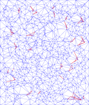
(a) Train mesh after model training for 1 epoch

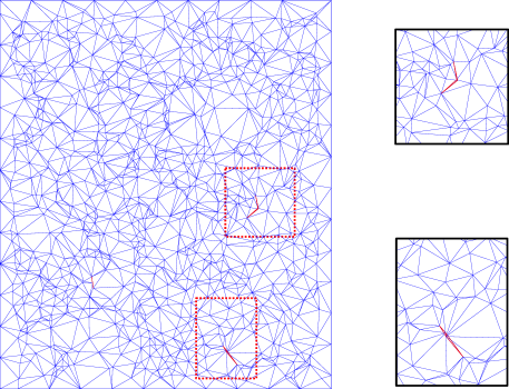
(b) Train mesh after model training for 10 epochs

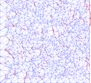
(c) Test mesh after model training for 1 epoch

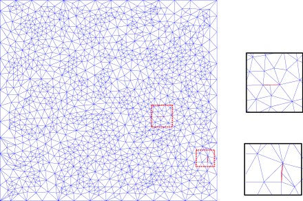
(d) Test mesh after model training for 10 epochs

Figure 8: The essential of shift truncation. The red elements in the figure represent negative volume elements.

To compare the effectiveness of shift truncation in the model, we visualized the output mesh after the first epoch of training. It can be observed that a large portion of the node updates resulted in negative volume elements, as shown in Figure 8a. However, as the model continues training, it learns the smoothing process, and the number of negative volume elements decreases, as depicted in Figure 8b. We also study the impact of shift truncation in the model predictions. The experimental results are shown in Figure 8c and 8c. It is evident that for certain highly distorted elements, the model may produce negative volume elements despite being trained for epochs. This demonstrates that shift truncation is essential during the prediction stage.

4.4 The influence of different loss functions

In Section 3.2.3, we designed a loss function for model training. In this section, we discuss the effectiveness of MetricLoss and how to choose the appropriate loss function. We compare the performance of commonly used mesh quality metrics as loss functions during model training, including:

• Min-max angle loss:
  $\mathcal{L}(\boldsymbol{x},\mathbf{S}(\boldsymbol{x}))=\frac{1}{|\mathbf{S}(\boldsymbol{x})|}\sum_{i=1}^{|\mathbf{S}(\boldsymbol{x})|}{\min\max(\theta_{ij})}$, for $j=1,2,3$, where $\theta_{ij}$ is the angle in triangle $T_{i}$.

• Aspect ratio loss:
  $\mathcal{L}(\boldsymbol{x},\mathbf{S}(\boldsymbol{x}))=\frac{1}{|\mathbf{S}(\boldsymbol{x})|}\sum_{i=1}^{|\mathbf{S}(\boldsymbol{x})|}{\frac{m_{i}^{2}+n_{i}^{2}+l_{i}^{2}}{4\sqrt{3}S_{i}}}$, where the symbols are defined in Section 3.2.3.

• Cosine loss:
  $\mathcal{L}(\boldsymbol{x},\mathbf{S}(\boldsymbol{x}))=\frac{1}{3|\mathbf{S}(\boldsymbol{x})|}\sum_{i=1}^{|\mathbf{S}(\boldsymbol{x})|}{(\cos(\theta_{ij})-\frac{1}{2})^{2}}$

• MetricLoss:
  $\mathcal{L}(\boldsymbol{x},\mathbf{S}(\boldsymbol{x}))=\frac{1}{|\mathbf{S}(\boldsymbol{x})|}\sum_{i=1}^{|\mathbf{S}(\boldsymbol{x})|}{(1-\frac{4\sqrt{3}S_{i}}{m_{i}^{2}+n_{i}^{2}+l_{i}^{2}})}$

Table 3: Comparison of cosine loss and proposed loss on Pipe and Square meshes

		Min. Angle		Max. Angle		$\frac{1}{\text{Aspect ratio}}$
Mesh	Algorithm	min	mean	max	mean	min	mean
Pipe	Cosine loss	26.77	55.71	110.43	64.67	0.54	0.95
	MetricLoss	26.37	55.56	107.73	64.82	0.56	0.95
Square	Cosine loss	11.04	43.76	146.87	79.61	0.25	0.79
	MetricLoss	13.53	44.06	150.46	79.65	0.22	0.79

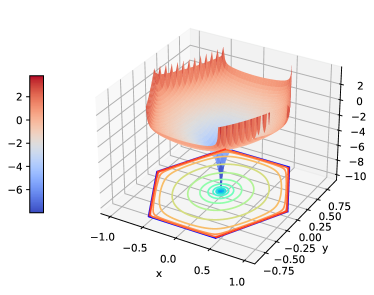
(a) Aspect ratio loss

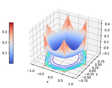
(b) Min-max angle loss

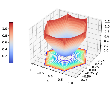
(c) Cosine loss

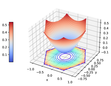
(d) The proposed loss

Figure 9: Plots of different loss functions. The range and smoothness of the loss function influence the model’s convergence. In Figure 9a, The z-coordinate is given as $log(z)$.

The plots of the aforementioned loss functions with respect to the variations in the central node of the StarPolygon are shown in Figure 9. It can be observed that the loss function we employed exhibits smoother transformations as the input changes, which facilitates the optimization process. We can also see than the aspect ratio loss and min-max angle loss are not suitable to be employed as the loss function. When encountering highly distorted elements, the former leads to numerical values approaching positive infinity, causing a sharp increase in loss and inducing training instability. The latter, on the other hand, results in abrupt changes in loss when facing highly distorted elements, while the loss function remains relatively flat when the central node is situated in the neighborhood of the optimal position. This circumstance also hinders the optimization process. Although the original angle-based loss function is difficult to train, the loss function transformed using the cosine function is more stable, as shown in Figure 9c. We trained the model using different loss functions, employing the same model configuration and training configuration. The train loss and validation loss of models with different loss functions are depicted in Figure 10. It can be observed that MetricLoss and cosine loss function are suitable for training the model, as the model converges rapidly after several iterations. Moreover, MetricLoss is remarkably stable during the training process. The experiments between two models based on different loss functions are shown in Table 3. It can be seen that the models show similar performance.

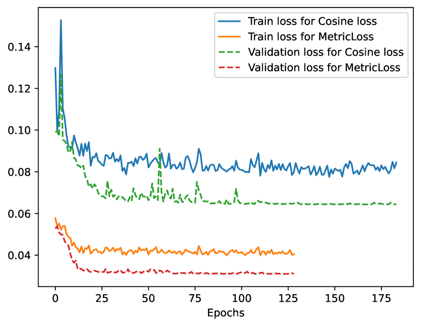
Figure 10: Comparison of different loss functions. The loss functions based on min-max angle and aspect ratio encountered training failures during the initial epochs. In contrast, both MetricLoss and the transformed Cosine loss function yielded convergent results.

When training with the other two loss functions, the model either fails to converge or exhibits severe oscillations. This indicates that employing mesh quality metrics with a larger range of numerical values or rapid changes in the numerical values when encountering highly distorted elements is detrimental to the training of the model. In summary, various loss functions can be used for mesh smoothing model training. When constructing the loss function through mesh quality metrics, it is necessary to consider the behavior of the function when encountering distorted elements, and to avoid selecting loss functions with a larger range of numerical values or abrupt changes. Inappropriate mesh quality metrics can also be transformed and employed for model training, as demonstrated by the min-max angle loss and cosine loss.

5 Conclusion

In this paper, we propose a graph neural network model, GMSNet, for intelligent mesh smoothing. The proposed model takes the neighbours of mesh nodes as input and learns to directly output the smoothed positions of mesh nodes, avoiding the computational overhead associated with the optimization-based smoothing. A fault-tolerance mechanism, shift truncation, is also applied to prevent negative volume elements. With a lightweight design, GMSNet can be applied to mesh nodes with varying degrees, and is not affected by the data input order. We also introduce an novel loss function, MetricLoss, based on mesh quality metrics, eliminating the need for high-quality mesh generation cost to train the model. Experiments on two-dimensional triangle meshes demonstrates that our proposed model achieves outstanding smoothing performance with an average acceleration of 8.62 times compared to to optimization-based smoothing. The results also show that GMSNet achieve superior performance than NN-Smoothing model with just 5% model parameters. We also illustrate that MetricLoss achieves fast and stable model training, and show the essential of shift truncation operation through experiments.

Future work includes applying our proposed method to other types of mesh elements and extending it to surface and volume meshes. Introducing edge flipping and mesh density modification into the mesh smoothing process to achieve superior mesh smoothing effects is also an approach worth exploring.

Supplementary information

Acknowledgments

This research work was supported in part by the National Key Research and Development Program of China (2021YFB0300101).

Declarations

References

- \bibcommenthead
- Spalart and Venkatakrishnan [2016] Spalart, P.R., Venkatakrishnan, V.: On the role and challenges of cfd in the aerospace industry. The Aeronautical Journal 120(1223), 209–232 (2016)
- Bridgeman et al. [2010] Bridgeman, J., Jefferson, B., Parsons, S.A.: The development and application of cfd models for water treatment flocculators. Advances in Engineering Software 41(1), 99–109 (2010)
- Damjanović et al. [2011] Damjanović, D., Kozak, D., Živić, M., Ivandić, Ž., Baškarić, T.: Cfd analysis of concept car in order to improve aerodynamics. Járműipari innováció 1(2), 108–115 (2011)
- Samstag et al. [2016] Samstag, R.W., Ducoste, J.J., Griborio, A., Nopens, I., Batstone, D., Wicks, J., Saunders, S., Wicklein, E., Kenny, G., Laurent, J.: Cfd for wastewater treatment: an overview. Water Science and Technology 74(3), 549–563 (2016)
- Darwish and Moukalled [2016] Darwish, M., Moukalled, F.: The Finite Volume Method in Computational Fluid Dynamics: an Advanced Introduction with OpenFOAM® and Matlab®, pp. 110–128. Springer, Berlin (2016)
- Baker [2005] Baker, T.J.: Mesh generation: Art or science? Progress in Aerospace Sciences 41(1), 29–63 (2005)
- Knupp [2001] Knupp, P.M.: Algebraic mesh quality metrics. SIAM journal on scientific computing 23(1), 193–218 (2001)
- Freitag and Ollivier-Gooch [1997] Freitag, L.A., Ollivier-Gooch, C.: Tetrahedral mesh improvement using swapping and smoothing. International Journal for Numerical Methods in Engineering 40(21), 3979–4002 (1997)
- Freitag and Ollivier-Gooch [1996] Freitag, L.A., Ollivier-Gooch, C.: A comparison of tetrahedral mesh improvement techniques. Technical report, Argonne National Lab.(ANL), Argonne, IL (United States) (1996)
- Prasad [2018] Prasad, T.: A comparative study of mesh smoothing methods with flipping in 2d and 3d. PhD thesis, Rutgers University-Camden Graduate School (2018)
- Guo et al. [2021] Guo, Y., Wang, C., Ma, Z., Huang, X., Sun, K., Zhao, R.: A new mesh smoothing method based on a neural network. Computational Mechanics, 1–14 (2021)
- Herrmann [1976] Herrmann, L.R.: Laplacian-isoparametric grid generation scheme. Journal of the Engineering Mechanics Division 102(5), 749–756 (1976)
- Zhou and Shimada [2000] Zhou, T., Shimada, K.: An angle-based approach to two-dimensional mesh smoothing. IMR 2000, 373–384 (2000)
- Du and Gunzburger [2002] Du, Q., Gunzburger, M.: Grid generation and optimization based on centroidal voronoi tessellations. Applied mathematics and computation 133(2-3), 591–607 (2002)
- Lloyd [1982] Lloyd, S.: Least squares quantization in pcm. IEEE transactions on information theory 28(2), 129–137 (1982)
- Du et al. [1999] Du, Q., Faber, V., Gunzburger, M.: Centroidal voronoi tessellations: Applications and algorithms. SIAM review 41(4), 637–676 (1999)
- Parthasarathy and Kodiyalam [1991] Parthasarathy, V., Kodiyalam, S.: A constrained optimization approach to finite element mesh smoothing. Finite Elements in Analysis and Design 9(4), 309–320 (1991)
- Field [1988] Field, D.A.: Laplacian smoothing and delaunay triangulations. Communications in applied numerical methods 4(6), 709–712 (1988)
- Canann et al. [1998] Canann, S.A., Tristano, J.R., Staten, M.L.: An Approach to Combined Laplacian and Optimization-Based Smoothing for Triangular, Quadrilateral, and Quad-Dominant Meshes. IMR 1, 479–94 (1998). Publisher: Citeseer
- Field [1988] Field, D.A.: Laplacian smoothing and delaunay triangulations. Communications in applied numerical methods 4(6), 709–712 (1988)
- Chen et al. [2020] Chen, X., Liu, J., Pang, Y., Chen, J., Chi, L., Gong, C.: Developing a new mesh quality evaluation method based on convolutional neural network. Engineering Applications of Computational Fluid Mechanics 14(1), 391–400 (2020)
- Wang et al. [2022] Wang, Z., Chen, X., Li, T., Gong, C., Pang, Y., Liu, J.: Evaluating mesh quality with graph neural networks. Engineering with Computers 38(5), 4663–4673 (2022)
- Chen et al. [2021] Chen, X., Liu, J., Gong, C., Li, S., Pang, Y., Chen, B.: Mve-net: An automatic 3-d structured mesh validity evaluation framework using deep neural networks. Computer-Aided Design 141, 103104 (2021)
- Zhang et al. [2020] Zhang, Z., Wang, Y., Jimack, P.K., Wang, H.: Meshingnet: A new mesh generation method based on deep learning. In: International Conference on Computational Science, pp. 186–198 (2020). Springer
- Zhang et al. [2021] Zhang, Z., Jimack, P.K., Wang, H.: Meshingnet3d: Efficient generation of adapted tetrahedral meshes for computational mechanics. Advances in Engineering Software 157, 103021 (2021)
- Daroya et al. [2020] Daroya, R., Atienza, R., Cajote, R.: Rein: Flexible mesh generation from point clouds. In: Proceedings of the IEEE/CVF Conference on Computer Vision and Pattern Recognition Workshops, pp. 352–353 (2020)
- Papagiannopoulos et al. [2021] Papagiannopoulos, A., Clausen, P., Avellan, F.: How to teach neural networks to mesh: Application on 2-d simplicial contours. Neural Networks 136, 152–179 (2021)
- Chen et al. [2022] Chen, X., Li, T., Wan, Q., He, X., Gong, C., Pang, Y., Liu, J.: Mgnet: a novel differential mesh generation method based on unsupervised neural networks. Engineering with Computers 38(5), 4409–4421 (2022)
- Bohn and Feischl [2021] Bohn, J., Feischl, M.: Recurrent neural networks as optimal mesh refinement strategies. Computers & Mathematics with Applications 97, 61–76 (2021)
- Paszyński et al. [2021] Paszyński, M., Grzeszczuk, R., Pardo, D., Demkowicz, L.: Deep learning driven self-adaptive hp finite element method. In: International Conference on Computational Science, pp. 114–121 (2021). Springer
- Tingfan et al. [2022] Tingfan, W., Xuejun, L., Wei, A., Huang, Z., Hongqiang, L.: A mesh optimization method using machine learning technique and variational mesh adaptation. Chinese Journal of Aeronautics 35(3), 27–41 (2022)
- Wallwork et al. [2022] Wallwork, J.G., Lu, J., Zhang, M., Piggott, M.D.: E2n: error estimation networks for goal-oriented mesh adaptation. arXiv preprint arXiv:2207.11233 (2022)
- Fidkowski and Chen [2021] Fidkowski, K.J., Chen, G.: Metric-based, goal-oriented mesh adaptation using machine learning. Journal of Computational Physics 426, 109957 (2021)
- Wu et al. [2020] Wu, Z., Pan, S., Chen, F., Long, G., Zhang, C., Philip, S.Y.: A comprehensive survey on graph neural networks. IEEE transactions on neural networks and learning systems 32(1), 4–24 (2020)
- Vollmer et al. [1999] Vollmer, J., Mencl, R., Mueller, H.: Improved laplacian smoothing of noisy surface meshes. In: Computer Graphics Forum, vol. 18, pp. 131–138 (1999). Wiley Online Library
- Xu et al. [2018] Xu, K., Gao, X., Chen, G.: Hexahedral mesh quality improvement via edge-angle optimization. Computers & Graphics 70, 17–27 (2018)
- Reddy [1976] Reddy, D.R.: Speech recognition by machine: A review. Proceedings of the IEEE 64(4), 501–531 (1976)
- LeCun et al. [2015] LeCun, Y., Bengio, Y., Hinton, G.: Deep learning. nature 521(7553), 436–444 (2015)
- Pak and Kim [2017] Pak, M., Kim, S.: A review of deep learning in image recognition. In: 2017 4th International Conference on Computer Applications and Information Processing Technology (CAIPT), pp. 1–3 (2017). IEEE
- Chowdhary and Chowdhary [2020] Chowdhary, K., Chowdhary, K.: Natural language processing. Fundamentals of artificial intelligence, 603–649 (2020)
- Kipf and Welling [2016] Kipf, T.N., Welling, M.: Semi-supervised classification with graph convolutional networks. arXiv preprint arXiv:1609.02907 (2016)
- Song et al. [2022] Song, W., Zhang, M., Wallwork, J.G., Gao, J., Tian, Z., Sun, F., Piggott, M., Chen, J., Shi, Z., Chen, X., et al.: M2n: mesh movement networks for pde solvers. Advances in Neural Information Processing Systems 35, 7199–7210 (2022)
- Lino et al. [2021] Lino, M., Cantwell, C., Bharath, A.A., Fotiadis, S.: Simulating continuum mechanics with multi-scale graph neural networks. arXiv preprint arXiv:2106.04900 (2021)
- Pfaff et al. [2020] Pfaff, T., Fortunato, M., Sanchez-Gonzalez, A., Battaglia, P.W.: Learning mesh-based simulation with graph networks. arXiv preprint arXiv:2010.03409 (2020)
- Han et al. [2022] Han, X., Gao, H., Pfaff, T., Wang, J.-X., Liu, L.-P.: Predicting physics in mesh-reduced space with temporal attention. arXiv preprint arXiv:2201.09113 (2022)
- Peng et al. [2022] Peng, W., Yuan, Z., Wang, J.: Attention-enhanced neural network models for turbulence simulation. Physics of Fluids 34(2) (2022)
- Li et al. [2019] Li, G., Muller, M., Thabet, A., Ghanem, B.: Deepgcns: Can gcns go as deep as cnns? In: Proceedings of the IEEE/CVF International Conference on Computer Vision, pp. 9267–9276 (2019)
- Cai et al. [2021] Cai, T., Luo, S., Xu, K., He, D., Liu, T.-y., Wang, L.: Graphnorm: A principled approach to accelerating graph neural network training. In: International Conference on Machine Learning, pp. 1204–1215 (2021). PMLR
- Ulyanov et al. [2016] Ulyanov, D., Vedaldi, A., Lempitsky, V.: Instance normalization: The missing ingredient for fast stylization. arXiv preprint arXiv:1607.08022 (2016)
- Kingma and Ba [2014] Kingma, D.P., Ba, J.: Adam: A method for stochastic optimization. arXiv preprint arXiv:1412.6980 (2014)
- Lee and Schachter [1980] Lee, D.-T., Schachter, B.J.: Two algorithms for constructing a delaunay triangulation. International Journal of Computer & Information Sciences 9(3), 219–242 (1980)