On the emergence of memory in equilibrium versus non-equilibrium systems

Abstract

Experiments often probe observables that correspond to low-dimensional projections of high-dimensional dynamics. In such situations distinct microscopic configurations become lumped into the same observable state. It is well known that correlations between the observable and the hidden degrees of freedom give rise to memory effects. However, how and under which conditions these correlations emerge remains poorly understood. Here we shed light on two fundamentally different scenarios of the emergence of memory in minimal stationary systems, where observed and hidden degrees of freedom evolve either cooperatively or are coupled by a hidden non-equilibrium current. In the reversible setting strongest memory manifests when the time-scales of hidden and observed dynamics overlap, whereas, strikingly, in the driven setting maximal memory emerges under a clear time-scale separation. Our results hint at the possibility of fundamental differences in the way memory emerges in equilibrium versus driven systems that may be utilized as a “diagnostic” of the underlying hidden transport mechanism.

Observables coupled to hidden degrees of freedom that do not relax sufficiently fast [1] or selected reaction coordinates that do not locally equilibrate in meso-states [2] generically display memory. In fact, this holds for most high-dimensional dynamics probed on a coarse-grained level [3, 4, 5, 6, 7, 8, 9, 10, 11, 12, 13, 14]. Tremendous progress has been made over the years in describing and understanding kinetic aspects of non-Markovian dynamics [15, 16, 17, 18, 19, 20, 21, 22, 23, 24, 25, 26, 27, 28, 29, 30, 31, 32, 1, 33, 34, 12, 35, 36, 37]. More recently, coarse-grained, partially observed dynamics have become of great interest from the point of view of thermodynamic inference [38, 39, 40, 41, 2, 42, 43, 44, 45, 46, 47, 48, 49, 50, 51, 52, 37]. Namely, while efficient methods exist to detect [53, 54, 55] and quantify [55] the existence of memory, it conversely turns out to be quite challenging to quantify [2, 42, 44, 56] or even infer [57, 50, 51, 37] irreversibility from lower-dimensional, projected dynamics. Thus, understanding potential differences in the emergence of memory in equilibrium and non-equilibrium systems is a difficult task.

Considering in particular ergodic dynamics in the sense that the probability distribution to be found in a given microscopic state at long times relaxes to a unique stationary, equilibrium or non-equilibrium, steady state from any initial condition, the extent of memory is necessarily finite and is more prominent if the hidden degrees of freedom are slow [1, 58, 2]. Yet, even in this “well behaved”, thermodynamically consistent [59] setting quite little is known about the possible ways in which the dynamics of observables can become correlated with that of hidden degrees of freedom on different time scales. A particularly intriguing question is whether there are any characteristic differences between how memory emerges in reversible versus irreversible, driven systems when observed dynamics is much faster than the hidden one.

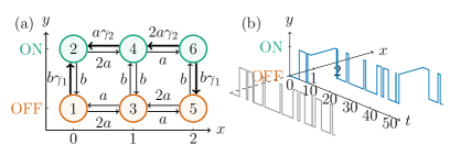
Figure 1: (a) Schematics of the full Markov network for the respective models. The upper green states are lumped to the observed “ON” state and the lower orange ones to the observed “OFF” state. In order to separate the time scale of horizontal and vertical dynamics, we choose the rates (in arbitrary units) $a=0.5$ and $b=25$ to make vertical process always much faster than horizontal one. In the driven model (see Fig. 2) we set $\gamma_{1}>1$ and $\gamma_{2}=1$, whereas in the reversible “allosteric” model (Fig. 3) we chose $\gamma_{1}=\gamma_{2}\equiv\gamma\geq 1$. A trajectory of the full dynamics (blue) and its corresponding projection (gray) are shown in panel (b).

Addressing this problem in full generality is a daunting task. Here we focus on the minimal “cooperative” setting [60, 61, 62, 63], where the microscopic dynamics is a Markov process on a planar network and we observe only the vertical coordinate whereas the horizontal transitions are hidden (see Fig. 1). This particular setting is important for understanding “active secondary transport”—transporter proteins exploiting the energy stored in transmembrane gradient of one type of molecules to transport another type against their gradients [64, 65, 66]. Moreover, it is also relevant as the physical basis of the sensitivity of the flagellar motor in E. coli in sensing concentrations of its regulator [60, 61, 62, 67], where two fundamentally different explanations were proposed to explain the “ultrasensitivity” of the motor’s response, an equilibrium allosteric and a dissipative non-equilibrium model [61, 67, 68].

We are not interested in the biophysical implications of the model. Instead, we use the above two distinct settings merely as a minimal model of non-Markovian 2-state dynamics, where we can “turn on” memory in a controlled manner via an equilibrium versus non-equilibrium mechanism. We consider the scenario, where the observed dynamics is faster than the hidden (see Fig. 1a) but there is not necessarily a large time-scale separation present. Interestingly, in the driven setting we only change the fastest time scales, whereas in the reversible cooperative model we alter all time scales. In both cases we find a maximal capacity for memory, i.e. the maximal magnitude of memory saturates at a finite coupling and non-equilibrium driving, respectively. Interestingly, in the reversible setting the memory manifests strongest when the time-scale separation between hidden and observed transition becomes partially lifted and the hidden and observable time-scales overlap, whereas in the driven setting maximal memory occurs in the presence of a time-scale separation. Our results provide deeper insight into the emergence of memory in the distinct situations when observed and hidden dynamics either evolve cooperatively or become coupled by a hidden non-equilibrium current.

Setup.—We consider a 6-state continuous-time Markov process (see Fig. 1a) with generator $L$, whose elements $L_{n,m}$ are transition rates between states $m\to n$ given by

$$L=\displaystyle{\begin{pmatrix}\ -b\gamma_{1}-2a&b&a&0&0&0\\ b\gamma_{1}&-b-2a&0&a\gamma_{2}&0&0\\ 2a&0&-b-2a&b&2a&0\\ 0&2a&b&-b-a-a\gamma_{2}&0&2a\gamma_{2}\\ 0&0&a&0&-b-2a&b\gamma_{1}\\ 0&0&0&a&b&-b\gamma_{1}-2a\gamma_{2}\end{pmatrix}},$$ (1)

where we choose $a=1/2$ and $b=25$ such that in the “baseline” model horizontal transitions are slower than vertical ones, i.e. the hidden dynamics relax slower than the observable ON$\rightleftarrows$OFF transitions. We adopt the Dirac bra-ket notation and denote the transition probability from microscopic state $i$ to microscopic state $j$ in time $t$ as $G(j,t|i)\equiv\langle j|\mathrm{e}^{Lt}|i\rangle$ and the stationary probability of state $j$ as $P_{s}(j)=\lim_{t\to\infty}G(j,t|i)$. In the baseline model with $\gamma_{1}=\gamma_{2}=1$ the dynamics is reversible and the ON/OFF states are equi-probable in the steady state. The parameters $\gamma_{1}$ and $\gamma_{2}$ are acceleration factors when they are larger than 1. In the cooperative allosteric regime with $\gamma_{1}=\gamma_{2}\equiv\gamma>1$ the dynamics obeys detailed balance, i.e. $P_{s}(i)L_{j,i}=P_{s}(j)L_{j,i},\,\forall i,j$. Conversely, in the driven model we set $\gamma_{1}>1,\gamma_{2}=1$; here detailed balance is violated, i.e. $\exists i,j$ for which $P_{s}(i)L_{j,i}\neq P_{s}(j)L_{j,i}$. (that is, the model is irreversible yet thermodynamically consistent [59]).

It turns out that $L$ defined this way is diagonalizable, i.e. we can find a bi-orthonormal basis $\{\langle\psi_{k}^{L}|,|\psi_{k}^{R}\rangle\}$ of left $\langle\psi_{k}^{L}|$ and right $|\psi_{k}^{R}\rangle$ eigenvectors with eigenvalue $-\lambda_{k}$ and $k=0,\ldots,5$ and $\langle\psi_{k}^{L}|\psi_{l}^{R}\rangle=\delta_{kl}$. Thus, we have $L=\sum_{k}-\lambda_{k}|\psi_{k}^{R}\rangle\langle\psi_{k}^{L}|$ and in turn we can expand $G(j,t|i)=\sum_{k=0}^{5}\langle j|\psi_{k}^{R}\rangle\langle\psi_{k}^{L}|i\rangle e^{-\lambda_{k}t}$. In this notation the steady-state probability of state $i$ is given by $P_{s}(i)=\langle i|\psi_{0}^{R}\rangle$.

The eigenvalues of the baseline model are $\lambda_{0}=0,\lambda_{1}=2a,\lambda_{2}=4a,\lambda_{3}=2b,\lambda_{4}=2(a+b),\lambda_{5}=2(2a+b)$. We can also determine the eigenspectrum analytically for the driven model, which has eigenvalues $\lambda^{\gamma_{1}}_{0}=0,\lambda^{\gamma_{1}}_{1}=2a,\lambda^{\gamma_{1}}_{2}=4a,\lambda^{\gamma_{1}}_{3}=\frac{1}{2}[4a+(\gamma_{1}+3)b-\sqrt{16a^{2}+(\gamma_{1}-1)^{2}b^{2}}],\lambda^{\gamma_{1}}_{4}=2a+(\gamma_{1}+1)b,\lambda^{\gamma_{1}}_{5}=\frac{1}{2}[4a+(\gamma_{1}+3)b+\sqrt{16a^{2}+(\gamma_{1}-1)^{2}b^{2}}]$. The reversible allosteric model ($\gamma>1$) cannot be diagonalized analytically and we therefore provide numerical results instead.

We assume that the full system is prepared in a steady state $P_{s}(j)$ and only vertical ON$\rightleftarrows$OFF transitions are observed with observable sets ${\rm ON}=\{2,4,6\}$ and ${\rm OFF}=\{1,3,5\}$. We determine the non-Markovian transition probability of the observed process $\hat{k}_{t}$, $Q_{P_{s}}(\hat{n},t|\hat{m})$ with $\hat{m},\hat{n}\in\{{\rm ON},{\rm OFF}\}$ as [1]

$$Q_{P_{s}}(\hat{n},t|\hat{m})\equiv\frac{\sum_{j=1}^{6}\mathbbm{1}_{\hat{n}}[j]\sum_{i=1}^{6}\mathbbm{1}_{\hat{m}}[i]G(j,t|i)P_{s}(i)}{\sum_{i=1}^{6}\mathbbm{1}_{\hat{m}}[i]P_{s}(i)},$$ (2)

where $\mathbbm{1}_{\Omega}$ is the indicator function of the set $\Omega$. The non-Markovian transition probability between two fixed observed states $\hat{m}\to\hat{n}$ as well as the observable return probability $\hat{m}\to\hat{m}$ depend on the preparation of the full system [69]. Moreover, in spite of the full system being prepared in the stationary state $P_{s}$, by specifying the initial observed state (here either “ON” or “OFF”) we “quench” the full system out of the steady state by conditioning on the state of the observable [1, 69]. Without loss of generality we will focus on the scenario where the observable is initially in the ON state, i.e. $\hat{k}_{0}={\rm ON}$.

To quantify the magnitude of memory in the projected dynamics, we follow [55] and construct the auxiliary Chapman-Kolmogorov (CK) transition density

$$Q^{\rm CK}(\hat{n},t_{1}+t_{2}|\hat{m})\equiv\sum_{\hat{k}}Q_{P_{s}}(\hat{n},t_{2}|\hat{k})Q_{P_{s}}(\hat{k},t_{1}|\hat{m}).$$ (3)

Note that for a non-Markovian process $Q^{\rm CK}$ depends on both $t_{1}$ and $t_{2}$. The Chapman-Kolmogorov construction $Q^{\rm CK}(\hat{n},t_{1}+t_{2}|\hat{m})$ corresponds to a fictitious dynamics where we force at time $t_{1}$ all hidden degrees of freedom to their stationary distribution and thereby erase all memory of their initial condition. When the observed ON$\rightleftarrows$OFF dynamics is Markovian we have $Q^{\rm CK}(\hat{n},t_{1}+t_{2}|\hat{m})=Q_{P_{s}}(\hat{n},t_{1}+t_{2}|\hat{m}),\,\forall t_{1},t_{2}\geq 0$ but the converse is not true in general [1, 55]. As soon as $Q^{\rm CK}(\hat{n},t_{1}+t_{2}|\hat{m})\neq Q_{P_{s}}(\hat{n},t_{1}+t_{2}|\hat{m})$ for some $\hat{n}$, the observable at time $t_{1}+t_{2}$ “remembers” the state of hidden degrees of freedom at time $t_{1}$.

We use the Kullback-Leibler divergence $D_{k}[p||q]\equiv\sum_{k}p(k)\ln[p(k)/q(k)]\geq 0$ to quantify the difference between $Q_{P_{s}}$ and $Q^{\rm CK}$ [55]

$$D_{\hat{m}}^{\rm CK}(t_{1},t_{2})\equiv D_{\hat{n}}[Q_{P_{s}}(\hat{n},t_{1}+t_{2}|\hat{m})||Q^{\rm CK}(\hat{n},t_{1}+t_{2}|\hat{m})],$$ (4)

where the superscript $k$ in $D_{k}[p||q]$ denotes the independent dummy variable of the measures $p$ and $q$. In the absence of memory $D_{\hat{m}}^{\rm CK}(t_{1},t_{2})=0,\,\forall t_{1},t_{2}$. Conversely, as we are interested in ergodic dynamics prepared in a steady state, we have that $D_{\hat{m}}^{\rm CK}\to 0$ whenever $t_{1}+t_{2}\to 0$ or $t_{1}+t_{2}\to\infty$ [55]. Therefore, by the positivity of $D_{\hat{m}}^{\rm CK}$ we will have at least one maximum in the half-space to $t_{1},t_{2}>0$. We quantify the magnitude of memory in terms of the global maximum on $t_{1},t_{2}>0$

$$D_{\rm max}^{\rm CK}(\hat{m})\equiv\sup_{t_{1},t_{2}>0}D_{\hat{m}}^{\rm CK}(t_{1},t_{2}).$$ (5)

In the baseline setting ($\gamma_{1}=\gamma_{2}=1$) the observed and hidden dynamics are decoupled (i.e. all microscopic pathways are equivalent). As a result, the observed dynamics is Markovian and $D_{\rm max}^{\rm CK}(\hat{m})=0$. We are interested in the dependence of $D_{\rm max}^{\rm CK}(\hat{m})$ as we couple the vertical and horizontal dynamics cooperatively or by a dissipative current, that is, on $\gamma_{1}$ and $\gamma$ in the driven and cooperative model, respectively.

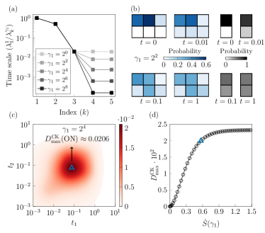
Figure 2: Driven setting ($\gamma_{1}>1,\gamma_{2}=1$): (a) Characteristic time-scales $1/\lambda_{i}^{\gamma_{1}},\,i\geq 1$ as a function of $\gamma_{1}$ relative to the baseline relaxation time $1/\lambda^{1}_{1}$. (b) Left: Microscopic transition probability $G(j,t|{\rm ON})$ for $\gamma_{1}=2^{2}$ at four different times. Right: Corresponding observed transition probability $Q_{P_{s}}(\hat{n},t|\rm ON)$. (c) Relative entropy $D_{\rm ON}^{\rm CK}(t_{1},t_{2})$ in Eq. (4) for $\gamma_{1}=2^{4}$; The triangle depicts $D^{\text{CK}}_{\rm max}({\rm ON})$. (d) Magnitude of memory $D^{\text{CK}}_{\rm max}({\rm ON})$ in Eq. (5) as a function of driving $\dot{S}(\gamma_{1})$; the blue triangle denotes the position of maximum in (c).

Driven setting.—We first consider the driven scenario with $\gamma_{1}>1$ and $\gamma_{2}=1$. Instead of $\gamma_{1}$ we use the steady-state entropy production rate of the microscopic dynamics $\dot{S}(\gamma_{1})=\sum_{i,j}P_{s}(j)L_{i,j}\ln[P_{s}(j)L_{i,j}/(P_{s}(i)L_{j,i})]$ to indicate how far the system is driven out of equilibrium and we change $\gamma$ in equidistant units of the chemical potential $\ln(\gamma_{1}/\gamma_{2})=\ln\gamma_{1}$ that drives the system out of equilibrium, i.e. $\gamma$ increases exponentially. We first provide some intuition about the microscopic dynamics.

Since $\lambda_{1,2}$ are independent of $\gamma_{1}$ and because $\lambda_{3}\simeq 2(a+b)$ for $b\gg a$ and $\gamma_{1}\geq 2$, by increasing $\gamma_{1}$ we only alter $\lambda_{4,5}$ (see Fig. 2a and Appendix B). That is, we are essentially only tuning the fastest time scales, whereas the slow time scales remain unaffected by the driving. We also alter the stationary distribution $P_{s}(\hat{m})$. Because $b\gg a$ the system (even without driving) tends to first explore vertical paths to reach a “quasi-steady state” between observed ON-OFF states within a time scale of approximately $\sim 1/b=0.04$ (see Fig. 2b). Afterwards, the probability redistributes horizontally within observable states. However, because the transition rates from state 1 to 2 and from 6 to 5 are accelerated by a factor of $\gamma_{1}$, transitions $2\to 1$ and $6\to 5$ will be instantly followed by the reverse transitions $1\to 2$ and $5\to 6$. Thus, the probability distribution dominantly redistributes along the microscopic path $2\leftrightarrow 4\leftrightarrow 3\leftrightarrow 5$, and finally reaches a steady state “skewed” in the hidden direction (see Fig. 2b).

We now address the magnitude of the emerging memory via $D^{\rm CK}_{\rm max}$ in Eq. (5). We find that $D^{\rm CK}_{\rm max}$ monotonically increases with $\gamma_{1}$ (note that $\dot{S}$ is a monotonically increasing function of $\gamma_{1}$), and eventually at $\approx 0.02324$, where the location of the supremum approaches $t_{1}=t_{2}\approx 0.08$ as $\gamma_{1}\to\infty$. Note that the maximal memory is attained on a time scale that is longer than the local vertical equilibration time $\approx 1/b=0.04$. The saturation may be explained by noticing that as $\gamma_{1}\to\infty$, only states $2,3,4,5$ have a non-zero probability and accelerated paths are almost never traversed. As a result, $D^{\rm CK}_{\rm max}$ no longer changes with $\gamma_{1}$.

Note that in this driven setting vertical transitions are always much faster than horizontal ones, which maintains a separation of time scales between observed and hidden dynamics. The memory we observe is thus “only” a manifestation of the relaxation of hidden degrees of freedom.

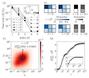
Figure 3: Reversible setting ($\gamma_{1}=\gamma_{2}=\gamma$): (a) Characteristic time-scales $1/\lambda_{i}^{\gamma},\,i\geq 1$ as a function of $\gamma_{1}=\gamma_{2}=\gamma$ relative to the baseline relaxation time $1/\lambda^{1}_{1}$. Inset: $\lambda^{1}_{1}/\lambda_{1}^{\gamma}$ on a linear scale. (b) Left: Microscopic transition probability $G(j,t|{\rm ON})$ for $\gamma=2^{2}$ at four different times. Right: Corresponding observed transition probability $Q_{P_{s}}(\hat{n},t|\rm ON)$. (c) Relative entropy $D_{\rm ON}^{\rm CK}(t_{1},t_{2})$ in Eq. (4) for $\gamma=2^{4}$ as a function of $t_{1},t_{2}$; The triangle denotes $D^{\text{CK}}_{\rm max}({\rm ON})$. (d) Magnitude of memory $D^{\text{CK}}_{\rm max}({\rm ON})$ in Eq. (5) as a function of $\gamma$.

Reversible cooperative setting.—We now inspect the reversible scenario where $\gamma_{1}=\gamma_{2}\equiv\gamma\geq 1$. As before, we first give some insight into the microscopic dynamics. As time evolves, in the first stage the system initially populates microscopic states 2 and 4, when $\gamma$ is large especially state 2. The accelerated transition paths do not instantly play a role. Thus, similar to the driven model, the system tends to first explore vertical paths (paths $2\to 1$ and $4\to 3$) on a time scale of $1/b\sim 0.04$. In the second stage, also similar to the driven model, transitions $2\to 1$ will instantly go back to state 2. During this stage, the probability redistributes in the horizontal direction. However, since the transition rates inside the ON state ($L_{2,4},L_{4,6}$) are also accelerated by a factor of $\gamma$, the time scale of the horizontal redistribution of probability is not necessarily larger than that of vertical dynamics. Here, the two main frequently visited vertical paths are $2\to 1$ and $4\to 3$.

Note that when we increase $\gamma$ in this reversible setting, such that $a\gamma>b$, part of the horizontal transition rates exceeds vertical ones, i.e. the time scales of observable dynamics and hidden dynamics overlap and there is no time-scale separation. This overlapping (and “mixing”) of hidden and observable time scales may contribute to the appearance of two shoulders in Fig. 3d at $\gamma\approx 38$ and $\gamma\approx 443$. The shoulders are a result of the shift in position of the peak of $D_{\hat{m}}^{\rm CK}(t_{1},t_{2})$ (for details see Fig. A1 in the Appendix A). As $\gamma$ tends to become very large, $D_{\rm max}^{\rm CK}$ saturates to $\approx 0.08471$, and the location of peak approaches $t_{1}=t_{2}\approx 0.13$.

Conclusion.—In this Letter we addressed the emergence of memory in a minimal setting, where the microscopic dynamics corresponds to a Markov process on a planar network and we observe only the vertical ON$\rightleftarrows$OFF dynamics, whereby the horizontal dynamics are hidden. Our aim was to gain insight into how correlations between hidden and observed dynamics emerge, in particular if and how the nature of these correlations depends on whether the microscopic dynamics is reversible (i.e. obeys detailed balance) or instead is driven. In the former scenario, the observed and hidden degrees of freedom are coupled cooperatively, whereas in the latter scenario the coupling emerges due to a non-equilibrium current. We focused on quantifying the magnitude of memory while tuning cooperativity or irreversible driving. Many features were found to be similar in both setting. However, in the reversible setting the strongest memory was found in the expected situation, when the time-scales of hidden and observed dynamics overlap. Conversely, in the driven setting maximal memory is reached under a clear time-scale separation. Our work therefore unravels qualitative differences in the way memory can emerge in equilibrium versus driven systems. While we focused on a simple model, our findings pave the way for more systematic studies. From a practical, “diagnostic” perspective, our results imply the possibility to gain insight about the dynamic coupling underlying active secondary transport [64, 65, 66] from observations of memory in the transmembrane transport of either species.

Acknowledgments.—Financial support from the Max Planck School Matter to Life supported by the German Federal Ministry of Education and Research (BMBF) in collaboration with the Max Planck Society (fellowship to XZ), and from the European Research Council (ERC) under the European Union’s Horizon Europe research and innovation programme (grant agreement No 101086182 to AG) is gratefully acknowledged.

Appendix A: Peak position of $D^{\rm CK}$ in the reversible setting.— Let $(t_{1}^{*},t_{2}^{*})\equiv{\rm arg\,max}_{t_{1},t_{2}}D_{\hat{m}}^{\rm CK}(t_{1},t_{2})$ be the values of $t_{1}$ and $t_{2}$ when $D_{\rm ON}^{\rm CK}$ reaches its maximum at a given $\gamma$ in the reversible cooperative scenario (see Fig. 3c). As stated in the main text, the two shoulders in Fig. 3d are a result of discontinuities in the shift of peak position. To visualize this, we show in Fig. A1 the dependence of the peak position on $\gamma$. Note that $G^{\rm CK}$ in Eq. (3) is a symmetric function of $t_{1}$ and $t_{2}$, so the peak of $D_{\rm ON}^{\rm CK}$ always occurs at $t_{1}^{*}=t_{2}^{*}$.

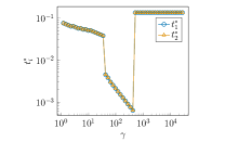
Figure A1: Dependence of the peak position of $D_{\rm ON}^{\rm CK}$, $(t_{1}^{*},t_{2}^{*})$, on the cooperativity parameter $\gamma$ in the reversible model. Note the two discontinuities.

Appendix B: Table of characteristic time-scales.— Table B1 lists a part of the characteristic time-scales under the driven and reversible settings shown in Figs. 2a and 3a, respectively.

Table B1: Characteristic time-scales relative to the baseline relaxation time in driven ($\lambda_{1}^{1}/\lambda_{k}^{\gamma_{1}}$) and reversible ($\lambda_{1}^{1}/\lambda_{k}^{\gamma}$) settings.

	Baseline	Driven ($\gamma_{1}>1,\gamma_{2}=1$)		Reversible ($\gamma_{1}=\gamma_{2}=\gamma$)
Index $k$	$\gamma_{1}=\gamma_{2}=1$	$\gamma_{1}=2^{4}$	$\gamma_{1}=2^{8}$	$\gamma=2^{4}$	$\gamma=2^{8}$
1	1	1	1	0.578	0.519
2	0.5	0.5	0.5	0.181	0.0465
3	0.02	0.0196	0.0196	0.0182	$6.29\times 10^{-3}$
4	0.0196	$2.35\times 10^{-3}$	$1.56\times 10^{-4}$	$2.35\times 10^{-3}$	$1.56\times 10^{-4}$
5	0.0192	$2.35\times 10^{-3}$	$1.56\times 10^{-4}$	$2.27\times 10^{-3}$	$1.50\times 10^{-4}$

References

- Lapolla and Godec [2019] A. Lapolla and A. Godec, Manifestations of projection-induced memory: General theory and the tilted single file, Front. Phys. 7, 10.3389/fphy.2019.00182 (2019).
- Hartich and Godec [2021a] D. Hartich and A. Godec, Emergent memory and kinetic hysteresis in strongly driven networks, Phys. Rev. X 11, 041047 (2021a).
- Plotkin and Wolynes [1998] S. S. Plotkin and P. G. Wolynes, Non-markovian configurational diffusion and reaction coordinates for protein folding, Phys. Rev. Lett. 80, 5015 (1998).
- Min et al. [2005] W. Min, G. Luo, B. J. Cherayil, S. C. Kou, and X. S. Xie, Observation of a power-law memory kernel for fluctuations within a single protein molecule, Phys. Rev. Lett. 94, 198302 (2005).
- Neusius et al. [2008] T. Neusius, I. Daidone, I. M. Sokolov, and J. C. Smith, Subdiffusion in peptides originates from the fractal-like structure of configuration space, Phys. Rev. Lett. 100, 188103 (2008).
- Sangha and Keyes [2009] A. K. Sangha and T. Keyes, Proteins Fold by Subdiffusion of the Order Parameter, J. Phys. Chem. B 113, 15886 (2009).
- Avdoshenko et al. [2017] S. M. Avdoshenko, A. Das, R. Satija, G. A. Papoian, and D. E. Makarov, Theoretical and computational validation of the Kuhn barrier friction mechanism in unfolded proteins, Sci. Rep. 7, 269 (2017).
- Makarov [2013] D. E. Makarov, Interplay of non-markov and internal friction effects in the barrier crossing kinetics of biopolymers: Insights from an analytically solvable model, J. Chem. Phys. 138, 014102 (2013).
- Ozmaian and Makarov [2019] M. Ozmaian and D. E. Makarov, Transition path dynamics in the binding of intrinsically disordered proteins: A simulation study, J. Chem. Phys. 151, 235101 (2019).
- Meyer et al. [2020] H. Meyer, P. Pelagejcev, and T. Schilling, Non-markovian out-of-equilibrium dynamics: A general numerical procedure to construct time-dependent memory kernels for coarse-grained observables, EPL (Europhys. Lett.) 128, 40001 (2020).
- Pyo and Woodside [2019] A. G. T. Pyo and M. T. Woodside, Memory effects in single-molecule force spectroscopy measurements of biomolecular folding, Phys. Chem. Chem. Phys. 21, 24527–24534 (2019).
- Ayaz et al. [2022] C. Ayaz, L. Scalfi, B. A. Dalton, and R. R. Netz, Generalized langevin equation with a nonlinear potential of mean force and nonlinear memory friction from a hybrid projection scheme, Phys. Rev. E 105, 054138 (2022).
- Ginot et al. [2022] F. Ginot, J. Caspers, M. Krüger, and C. Bechinger, Barrier crossing in a viscoelastic bath, Phys. Rev. Lett. 128, 028001 (2022).
- Narinder et al. [2018] N. Narinder, C. Bechinger, and J. R. Gomez-Solano, Memory-induced transition from a persistent random walk to circular motion for achiral microswimmers, Phys. Rev. Lett. 121, 078003 (2018).
- Haken [1975] H. Haken, Cooperative phenomena in systems far from thermal equilibrium and in nonphysical systems, Rev. Mod. Phys. 47, 67 (1975).
- Grabert et al. [1977] H. Grabert, P. Talkner, and P. Hänggi, Microdynamics and time-evolution of macroscopic non-markovian systems, Z. Phys. B: Cond. Matt. 26, 389 (1977).
- Grabert et al. [1978] H. Grabert, P. Talkner, P. Hänggi, and H. Thomas, Microdynamics and time-evolution of macroscopic non-markovian systems. ii, Z. Phys. B: Cond. Matt. 29, 273–280 (1978).
- Casademunt et al. [1987] J. Casademunt, R. Mannella, P. V. E. McClintock, F. E. Moss, and J. M. Sancho, Relaxation times of non-markovian processes, Phys. Rev. A 35, 5183 (1987).
- Ferrario and Grigolini [2008] M. Ferrario and P. Grigolini, The non‐Markovian relaxation process as a “contraction” of a multidimensional one of Markovian type, J. Math. Phys. 20, 2567 (2008).
- Goychuk [2012] I. Goychuk, Viscoelastic subdiffusion: Generalized langevin equation approach, Adv. Chem. Phys. , 187–253 (2012).
- Sokolov [2002] I. M. Sokolov, Solutions of a class of non-Markovian Fokker-Planck equations, Phys. Rev. E 66, 041101 (2002).
- Sokolov [2003] I. M. Sokolov, Cyclization of a polymer: First-passage problem for a Non-Markovian process, Phys. Rev. Lett. 90, 080601 (2003).
- Dybiec et al. [2011] B. Dybiec, I. M. Sokolov, and A. V. Chechkin, Relaxation to stationary states for anomalous diffusion, Commun. Nonlinear Sci. Numer. Simul. 16, 4549–4557 (2011).
- Metzler and Klafter [2000] R. Metzler and J. Klafter, The random walk’s guide to anomalous diffusion: a fractional dynamics approach, Phys. Rep. 339, 1 (2000).
- Metzler and Klafter [2004] R. Metzler and J. Klafter, The restaurant at the end of the random walk: recent developments in the description of anomalous transport by fractional dynamics, J. Phys. A: Math. Gen. 37, R161 (2004).
- Barkai et al. [2000] E. Barkai, R. Metzler, and J. Klafter, From continuous time random walks to the fractional fokker-planck equation, Phys. Rev. E 61, 132 (2000).
- Schulz et al. [2014] J. H. P. Schulz, E. Barkai, and R. Metzler, Aging renewal theory and application to random walks, Phys. Rev. X 4, 011028 (2014).
- Carmi et al. [2010] S. Carmi, L. Turgeman, and E. Barkai, On distributions of functionals of anomalous diffusion paths, J. Stat. Phys. 141, 1071–1092 (2010).
- Barkai and Sokolov [2007] E. Barkai and I. M. Sokolov, Multi-point distribution function for the continuous time random walk, J. Stat. Mech. 2007, P08001 (2007).
- Bray et al. [2013] A. J. Bray, S. N. Majumdar, and G. Schehr, Persistence and first-passage properties in nonequilibrium systems, Adv. Phys. 62, 225 (2013), https://doi.org/10.1080/00018732.2013.803819 .
- Majumdar and Bray [1998] S. N. Majumdar and A. J. Bray, Persistence with partial survival, Phys. Rev. Lett. 81, 2626 (1998).
- Majumdar et al. [1996] S. N. Majumdar, A. J. Bray, S. J. Cornell, and C. Sire, Global persistence exponent for nonequilibrium critical dynamics, Phys. Rev. Lett. 77, 3704 (1996).
- Lapolla and Godec [2020] A. Lapolla and A. Godec, Single-file diffusion in a bi-stable potential: Signatures of memory in the barrier-crossing of a tagged-particle, J. Chem. Phys. 153, 194104 (2020).
- Talkner and Hänggi [2020] P. Talkner and P. Hänggi, Colloquium: Statistical mechanics and thermodynamics at strong coupling: Quantum and classical, Rev. Mod. Phys. 92, 041002 (2020).
- Di Terlizzi et al. [2020] I. Di Terlizzi, F. Ritort, and M. Baiesi, Explicit solution of the generalised langevin equation, J. Stat. Phys. 181, 1609–1635 (2020).
- Netz [2023a] R. R. Netz, Derivation of the non-equilibrium generalized langevin equation from a generic time-dependent hamiltonian (2023a), arXiv:2310.00748 [cond-mat.stat-mech] .
- Netz [2023b] R. R. Netz, Multi-point distribution for gaussian non-equilibrium non-markovian observables (2023b), arXiv:2310.08886 [cond-mat.stat-mech] .
- Terlizzi and Baiesi [2020] I. D. Terlizzi and M. Baiesi, A thermodynamic uncertainty relation for a system with memory, J. Phys. A: Math. Theor. 53, 474002 (2020).
- Mehl et al. [2012] J. Mehl, B. Lander, C. Bechinger, V. Blickle, and U. Seifert, Role of hidden slow degrees of freedom in the fluctuation theorem, Phys. Rev. Lett. 108, 220601 (2012).
- Esposito [2012] M. Esposito, Stochastic thermodynamics under coarse graining, Phys. Rev. E 85, 041125 (2012).
- van der Meer et al. [2022] J. van der Meer, B. Ertel, and U. Seifert, Thermodynamic inference in partially accessible markov networks: A unifying perspective from transition-based waiting time distributions, Phys. Rev. X 12, 031025 (2022).
- Harunari et al. [2022] P. E. Harunari, A. Dutta, M. Polettini, and E. Roldán, What to learn from a few visible transitions’ statistics?, Phys. Rev. X 12, 041026 (2022).
- Dieball and Godec [2022] C. Dieball and A. Godec, Mathematical, thermodynamical, and experimental necessity for coarse graining empirical densities and currents in continuous space, Phys. Rev. Lett. 129, 140601 (2022).
- van der Meer et al. [2023] J. van der Meer, J. Degünther, and U. Seifert, Time-resolved statistics of snippets as general framework for model-free entropy estimators, Phys. Rev. Lett. 130, 257101 (2023).
- Godec and Makarov [2023a] A. Godec and D. E. Makarov, Challenges in inferring the directionality of active molecular processes from single-molecule fluorescence resonance energy transfer trajectories, J. Phys. Chem. Lett. 14, 49 (2023a).
- Andrieux [2012] D. Andrieux, Bounding the coarse graining error in hidden markov dynamics, Appl. Math. Lett. 25, 1734 (2012).
- Gomez-Marin et al. [2008] A. Gomez-Marin, J. M. R. Parrondo, and C. Van den Broeck, Lower bounds on dissipation upon coarse graining, Phys. Rev. E 78, 011107 (2008).
- Rahav and Jarzynski [2007] S. Rahav and C. Jarzynski, Fluctuation relations and coarse-graining, J. Stat. Mech. 2007, P09012 (2007).
- Teza and Stella [2020] G. Teza and A. L. Stella, Exact coarse graining preserves entropy production out of equilibrium, Phys. Rev. Lett. 125, 110601 (2020).
- Roldán and Parrondo [2010] E. Roldán and J. M. R. Parrondo, Estimating dissipation from single stationary trajectories, Phys. Rev. Lett. 105, 150607 (2010).
- Roldán and Parrondo [2012] E. Roldán and J. M. R. Parrondo, Entropy production and kullback-leibler divergence between stationary trajectories of discrete systems, Phys. Rev. E 85, 031129 (2012).
- Baiesi et al. [2023] M. Baiesi, G. Falasco, and T. Nishiyama, Effective estimation of entropy production with lacking data (2023), arXiv:2305.04657 [cond-mat.stat-mech] .
- Berezhkovskii and Makarov [2018] A. M. Berezhkovskii and D. E. Makarov, Single-Molecule Test for Markovianity of the Dynamics along a Reaction Coordinate, J. Phys. Chem. Lett. 9, 2190 (2018).
- Engbring et al. [2023] K. Engbring, D. Boriskovsky, Y. Roichman, and B. Lindner, A nonlinear fluctuation-dissipation test for markovian systems, Phys. Rev. X 13, 021034 (2023).
- Lapolla and Godec [2021] A. Lapolla and A. Godec, Toolbox for quantifying memory in dynamics along reaction coordinates, Phys. Rev. Research 3, L022018 (2021).
- Hartich and Godec [2023] D. Hartich and A. Godec, Violation of local detailed balance upon lumping despite a clear timescale separation, Phys. Rev. Res. 5, L032017 (2023).
- Godec and Makarov [2023b] A. Godec and D. E. Makarov, Challenges in inferring the directionality of active molecular processes from single-molecule fluorescence resonance energy transfer trajectories, J. Phys. Chem. Lett. 14, 49 (2023b).
- Hartich and Godec [2021b] D. Hartich and A. Godec, Thermodynamic uncertainty relation bounds the extent of anomalous diffusion, Phys. Rev. Lett. 127, 080601 (2021b).
- Seifert [2012] U. Seifert, Stochastic thermodynamics, fluctuation theorems and molecular machines, Rep. Prog. Phys. 75, 126001 (2012).
- Monod et al. [1965] J. Monod, J. Wyman, and J.-P. Changeux, On the nature of allosteric transitions: A plausible model, J. Mol. Biol. 12, 88 (1965).
- Tu [2008] Y. Tu, The nonequilibrium mechanism for ultrasensitivity in a biological switch: Sensing by maxwell’s demons, Proc. Natl. Acad. Sci. 105, 11737–11741 (2008).
- Korobkova et al. [2006] E. A. Korobkova, T. Emonet, H. Park, and P. Cluzel, Hidden stochastic nature of a single bacterial motor, Phys. Rev. Lett. 96, 058105 (2006).
- Marzen et al. [2013] S. Marzen, H. G. Garcia, and R. Phillips, Statistical mechanics of monod–wyman–changeux (mwc) models, J. Mol. Biol. 425, 1433 (2013).
- Berlaga and Kolomeisky [2021] A. Berlaga and A. B. Kolomeisky, Molecular mechanisms of active transport in antiporters: Kinetic constraints and efficiency, J. Phys. Chem. Lett. 12, 9588–9594 (2021).
- Berlaga and Kolomeisky [2022a] A. Berlaga and A. B. Kolomeisky, Understanding mechanisms of secondary active transport by analyzing the effects of mutations and stoichiometry, J. Phys. Chem. Lett. 13, 5405–5412 (2022a).
- Berlaga and Kolomeisky [2022b] A. Berlaga and A. B. Kolomeisky, Theoretical study of active secondary transport: Unexpected differences in molecular mechanisms for antiporters and symporters, J. Chem. Phys. 156, 10.1063/5.0082589 (2022b).
- Hartich et al. [2015] D. Hartich, A. C. Barato, and U. Seifert, Nonequilibrium sensing and its analogy to kinetic proofreading, New J. Phys. 17, 055026 (2015).
- Owen et al. [2020] J. A. Owen, T. R. Gingrich, and J. M. Horowitz, Universal thermodynamic bounds on nonequilibrium response with biochemical applications, Phys. Rev. X 10, 011066 (2020).
- Lapolla et al. [2021] A. Lapolla, J. C. Smith, and A. Godec, Ubiquitous dynamical time asymmetry in measurements on materials and biological systems (2021), arXiv:2102.01666 [cond-mat.stat-mech] .