Transferring to Real-World Layouts:
A Depth-aware Framework for Scene Adaptation

Abstract

Scene segmentation via unsupervised domain adaptation (UDA) enables the transfer of knowledge acquired from source synthetic data to real-world target data, which largely reduces the need for manual pixel-level annotations in the target domain. To facilitate domain-invariant feature learning, existing methods typically mix data from both the source domain and target domain by simply copying and pasting the pixels. Such vanilla methods are usually sub-optimal since they do not take into account how well the mixed layouts correspond to real-world scenarios. Real-world scenarios are with an inherent layout. We observe that semantic categories, such as sidewalks, buildings, and sky, display relatively consistent depth distributions, and could be clearly distinguished in a depth map. Based on such observation, we propose a depth-aware framework to explicitly leverage depth estimation to mix the categories and facilitate the two complementary tasks, i.e., segmentation and depth learning in an end-to-end manner. In particular, the framework contains a Depth-guided Contextual Filter (DCF) for data augmentation and a cross-task encoder for contextual learning. DCF simulates the real-world layouts, while the cross-task encoder further adaptively fuses the complementing features between two tasks. Besides, it is worth noting that several public datasets do not provide depth annotation. Therefore, we leverage the off-the-shelf depth estimation network to generate the pseudo depth. Extensive experiments show that our proposed methods, even with pseudo depth, achieve competitive performance on two widely-used benchmarks, i.e. 77.7 mIoU on GTA$\rightarrow$Cityscapes and 69.3 mIoU on Synthia$\rightarrow$Cityscapes.

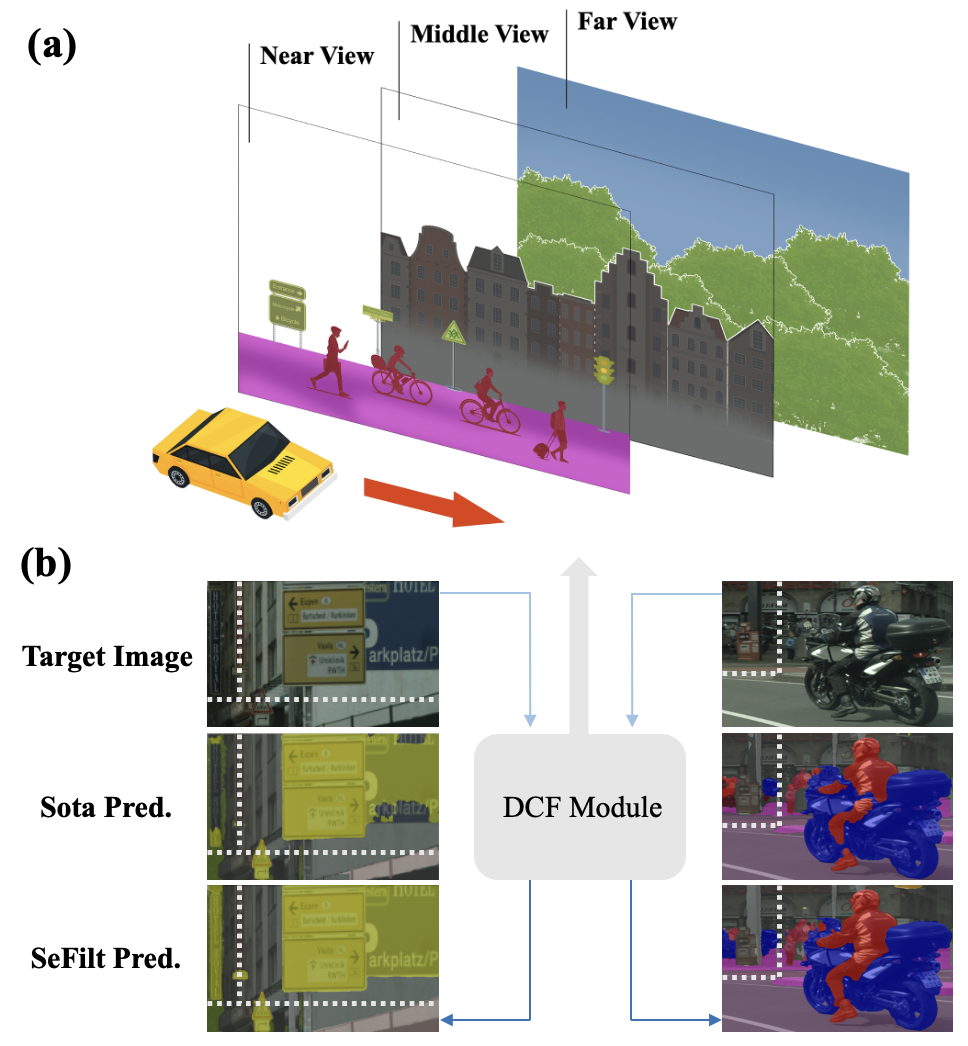
Figure 1: (a) Considering the driving scenario, we observe that the object location is relatively stable according to the distance from the camera. Therefore, we propose a Depth-guided Contextual Filter (DCF) which is aware of the semantic categories distribution in terms of Near, Middle, and Far view to facilitate cross-domain mixing. (b) Since we explicitly take the semantic layout into consideration, our method achieves better segmentation edges and yields significant improvement on small-scale categories such as Traffic Sign, Pole, and Rider, compared to the competitive MIC (second row) with the vanilla mixing strategy [1].

1 Introduction

Semantic segmentation refers to the task of assigning pixel-level category labels in an image, which has achieved significant progress in the last few years [2, 3, 4, 5]. It is worth noting that prevailing models usually require large-scale training datasets with high-quality annotations, such as ADE20K [6], to achieve good performance and but such pixel-level annotations in real-world are usually unaffordable and time-consuming [7]. One straightforward idea is to train networks with synthetic data so that the pixel-level annotations are easier to obtain [8, 9]. However, the network trained with synthetic data usually results in poor scalability when being deployed to a real-world environment due to multiple factors, such as weather, illumination, and road design. Therefore, researchers resort to unsupervised domain adaptation (UDA) to further tackle the variance between domains. One branch of UDA methods attempts to mitigate the domain shift by aligning the domain distributions [10, 11, 12, 13, 14]. Another potential paradigm to heal the domain shift is self-training [15, 16, 17, 18, 19], which recursively refine the target pseudo-labels. Taking one step further, recent DACS [20] and follow-up works [21, 22, 23, 1, 24, 25, 26] combine self-training and ClassMix [27] to mix images from both source and target domain. In this way, these works could craft highly perturbed samples to assist training by facilitating learning shared knowledge between two domains. Specifically, cross-domain mixing aims to copy the corresponding regions of certain categories from a source domain image and paste them onto an unlabelled target domain image. We note that such a vanilla strategy leads to pasting a large amount of objects to the unrealistic depth position. It is because that every category has its own position distribution. For instance, the background classes such as ”sky” and ”vegetation” usually appear farther away, while the classes that occupy a small number of pixels such as ”traffic signs” and ”pole”, usually appear closer as shown in Figure 1 (a). Such crafted training data compromise contextual learning, leading to sub-optimal location prediction performance, especially for small objects.

To address these limitations, we observe the real-world depth distribution and find that semantic categories are easily separated (disentangled) in the depth map since they follow a similar distribution under certain scenarios, e.g., urban. Therefore, we propose a new depth-aware framework, which contains Depth Contextual Filter (DCF) and a cross-task encoder. In particular, DCF removes unrealistic classes mixed with the real-world target training samples based on the depth information. On the other hand, multi-modal data could improve the performance of deep representations and the effective use of the deep multi-task features to facilitate the final predictions is crucial. The proposed cross-task encoder contains two specific heads to generate intermediate features for each task and an Adaptive Feature Optimization module (AFO). AFO encourages the network to optimize the fused multi-task features in an end-to-end manner. Specifically, the proposed AFO adopts a series of transformer blocks to capture the information that is crucial to distinguish different categories and assigns high weights to discriminative features and vice versa.

The main contributions are as follows: (1) We propose a simple Depth-Guided Contextual Filter (DCF) to accurately explicitly leverage the key semantic categories distribution hidden in the depth map, enhancing the realism of cross-domain information mixing and refining the cross-domain layout mixing. (2) We propose an Adaptive Feature Optimization module (AFO) that enables the cross-task encoder to exploit the discriminative depth information and embed it with the visual feature which jointly facilitates semantic segmentation and pseudo depth estimation. (3) Albeit simple, the effectiveness of our proposed methods has been verified by extensive ablation studies. Despite the pseudo depth, our method still achieves competitive accuracy on two commonly used scene adaptation benchmarks, namely 77.7 mIoU on GTA$\rightarrow$Cityscapes and 69.3 mIoU on Synthia$\rightarrow$Cityscapes.

2 Related Work

2.1 Unsupervised Domain Adaptation

Unsupervised domain adaptation (UDA) aims to train a model on a label-rich source domain and adapt the model to a label-scarce target domain. Some methods propose learning the domain-invariant knowledge by aligning the source and target distribution at different levels. For instance, AdaptSegNet [12], ADVENT [28], and CLAN [13] adversarially align the distributions in the feature space. CyCADA [10] diminishes the domain shift at both pixel-level and feature-level representation. DALN [29] proposes a discriminator-free adversarial learning network and leverages the predicted discriminative information for feature alignment. Both Wu et al. [11] and Yue et al. [30] learn domain-invariant features by transferring the input images into different styles, such as rainy and foggy, while Zhao et al. [31] and Zhang et al. [32] diversify the feature distribution via normalization and adding noise respectively. Another line of work refines pseudo-labels gradually under the iterative self-training framework, yielding competitive results. Following the motivation of generating highly reliable pseudo labels for further model optimization, CBST [15] adopts class-specific thresholds on top of self-training to improve the generated labels. Feng et al. [33] acquire pseudo labels with high precision by leveraging the group information. PyCDA [34] constructs pseudo-labels in various scales to further improve the training. Zheng et al. [35] introduce memory regularization to generate consistent pseudo labels. Other works propose either confidence regularization [16, 17] or category-aware rectification [36, 37] to improve the quality of pseudo labels. DACS [20] proposes a domain-mixed self-training pipeline to mix cross-domain images during training, avoiding training instabilities. Kim et al. [38], Li et al. [39] and Wang et al. [40] combine adversarial and self-training for further improvement. Chen et al. [41] establish a deliberated domain bridging (DDB) that aligns and interacts with the source and target domain in the intermediate space. SePiCo [24] and PiPa [25] adopt contrastive learning to align the domains. Liu et al. [42] addresses the label shift problem by adopting class-level feature alignment for conditional distribution alignment. Researchers also attempted to perform entropy minimization [28, 43], and image translation [44, 45]. consistency regularization[46, 47, 48, 49]. Recent multi-target domain adaptation (MTDA) methods enable a single model to adapt a labeled source domain to multiple unlabeled target domains [50, 51, 52]. However, the above methods usually ignore the rich multi-modality information, which can be easily obtained from the depth sensor and other sensors.

2.2 Depth Estimation and Multi-task Learning in Semantic Segmentation

Semantic segmentation and geometric information are shown to be highly correlated [53, 54, 55, 56, 57, 58, 59]. Recently depth estimation has been increasingly used to improve the learning of semantics within the context of multi-task learning, but the depth information should be exploited more precisely to help the domain adaptation. SPIGAN [60] pioneered the use of geometric information as an additional supervision by regularizing the generator with an auxiliary depth regression task. DADA [61] introduces an adversarial training framework based on the fusion of semantic and depth predictions to facilitate the adaptation. GIO-Ada [62] leverages the geometric information on both the input level and output level to reduce domain shift. CTRL [63] encodes task dependencies between the semantic and depth predictions to capture the cross-task relationships. CorDA [21] bridges the domain gap by utilizing self-supervised depth estimation on both domains. Wu et al. [64] propose to further support semantic segmentation by depth distribution density. Our work follows a similar spirit to leverage depth knowledge as auxiliary supervision. It is worth noting that our work is primarily different from existing works in the following two aspects: (1) from the data perspective, we explicitly delineate the depth distribution to refine data augmentation and construct realistic training samples to enhance contextual learning. (2) from the network perspective, our proposed multi-task learning network not only adopts auxiliary supervision for learning more robust deep representations but also facilitates the multi-task feature fusion by iterative deploying of transformer blocks to jointly learn the rich multi-task information for improving the final predictions.

3 Method

Algorithm 1 Depth-guided Contextual Filter Algorithm with Cross-Image Mixing and Self Training

0:  Source domain: $(\mathbf{x}^{S},\mathbf{y}^{S},\mathbf{z}^{S}\sim\mathbf{X}^{S},\mathbf{Y}^{S},\mathbf{Z}^{S})$, Target domain: $(\mathbf{x}^{T},\mathbf{z}^{T}\sim\mathbf{X}^{T},\mathbf{Z}^{T})$. Semantic network $\mathcal{F}_{\theta}$.

1:  Initialize network parameters $\theta$ randomly.

2:  for iteration = 1 to $n$ do

3:     $\hat{\mathbf{y}}^{T}\leftarrow\mathcal{F}_{\theta}\left(\mathbf{x}^{T}\right),$ Generate pseudo label

4:     Pre-calculate the density value $\mathbf{p}$ for each class $i$ at each depth interval from the target depth map $\mathbf{z}^{T}$,

5:     $\hat{\mathbf{y}}^{M}\leftarrow\mathcal{M}\odot\mathbf{y}^{S}+\left(1-\mathcal{M}\right)\odot\mathbf{\hat{y}}^{T},$ Randomly select $50\%$ categories and copy the category ground truth label from the source image to target pseudo label${\mathbf{x}}^{M}\leftarrow\mathcal{M}\odot\mathbf{x}^{S}+\left(1-\mathcal{M}\right)\odot\mathbf{{x}}^{T},$ Copy the corresponding category region from the source image to the target image

6:     Re-calculate the density value $\hat{\mathbf{p}}$ after the mixing,

7:     Calculate the depth density distribution difference before and after mixing,

8:     Filter the category once the difference exceeds the threshold,

9:     Re-generate the depth-aware binary mask $\mathcal{M}^{DCF},$

10:     $\hat{\mathbf{y}}^{F}\leftarrow\mathcal{M^{DCF}}\odot\mathbf{y}^{S}+\left(1-\mathcal{M^{DCF}}\right)\odot\hat{\mathbf{y}}^{T},$ Generate the filtered training samples with new DCF mask$\mathbf{x}^{F}\leftarrow\mathcal{M^{DCF}}\odot\mathbf{x}^{S}+\left(1-\mathcal{M^{DCF}}\right)\odot\mathbf{x}^{T},$

11:     Compute predictions $\bar{\mathbf{y}}^{S}\leftarrow argmax\left(\mathcal{F}_{\theta}\left(\mathbf{x}^{S}\right)\right),$ $\bar{\mathbf{y}}^{F}\leftarrow argmax\left(\mathcal{F}_{\theta}\left(\mathbf{x}^{F}\right)\right),$

12:     Compute loss for the batch:$\ell\leftarrow{\mathcal{L}}\left(\bar{\mathbf{y}}^{S},\mathbf{y}^{S},\bar{\mathbf{y}}^{F},\hat{\mathbf{y}}^{F}\right).$

13:     Compute $\nabla_{\theta}\ell$ by backpropagation.

14:     Perform stochastic gradient descent.

15:  end for

16:  return  $\mathcal{F}_{\theta}$

3.1 Problem Formulation

In the common UDA setting, label-rich synthetic data is used as source $S$ and label-scarce real-world data is treated as target $T$. For example, we have $n$ number of labeled training samples in the source domain, $\left\{\left(\mathbf{x}_{1}^{S},\mathbf{y}_{1}^{S},\mathbf{z}_{1}^{S}\right),\ldots,\left(\mathbf{x}_{n}^{S},\mathbf{y}_{n}^{S},\mathbf{z}_{n}^{S}\right)\right\}$ sampled from source domain data $\left\{\mathbf{X}^{S},\mathbf{Y}^{S},\mathbf{Z}^{S}\right\}$, where $\mathbf{x}_{i}^{S}$ and $\mathbf{y}_{i}^{S}$ are the $i$-th sample and corresponding ground truth for semantic segmentation. $\mathbf{z}_{i}^{S}$ is the label for the depth estimation task. Similarly, we have $m$ number of unlabeled target images sampled from target domain data $\left\{\mathbf{X}^{T},\mathbf{Z}^{T}\right\}$, which is denoted by $\left\{\left(\mathbf{x}_{1}^{T},\mathbf{z}_{1}^{T}\right),\ldots,\left(\mathbf{x}_{m}^{T},\mathbf{z}_{m}^{T}\right)\right\}$, where $\mathbf{x}_{i}^{T}$ is the i-th unlabeled sample in the target domain and $\mathbf{z}_{i}^{T}$ is the label for the depth estimation task. Since depth annotation is not supported by common public datasets, we adopt pseudo depth that can be easily generated by the off-the-shelf model [65].

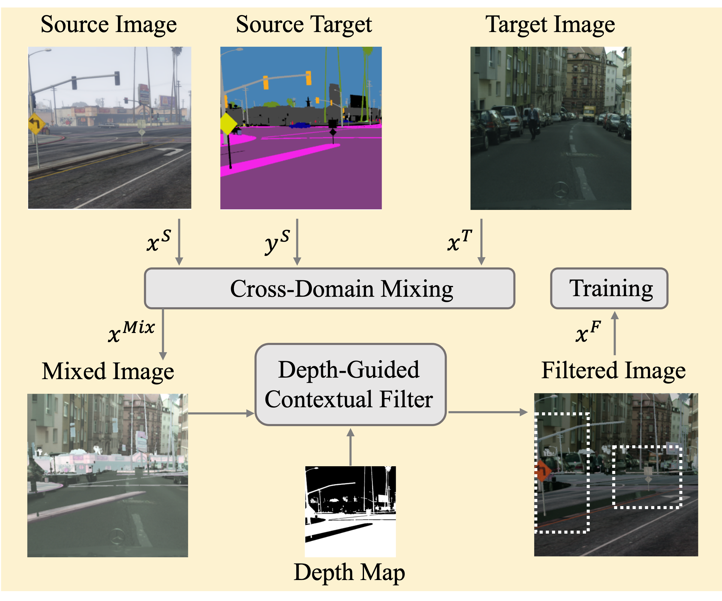
Figure 2: Source domain images $x^{S}$ and $x^{T}$ are mixed together, using the ground truth label $y^{S}$. The mixed images are de-noised by our proposed Depth-guided Contextual Filter (DCF) and then trained by the network. We illustrate DCF with a set of practical sample. As illustrated, the unrealistic “Building” pixels from the source image are mixed pasted to the target image, leading to a noisy mixed sample. The proposed DCF removes these pixels and maintain mixed pixels of “Traffic Sign” and “Pole” shown in the white dotted boxes, enhancing the realism of cross-domain mixing. (Best viewed when zooming in.)

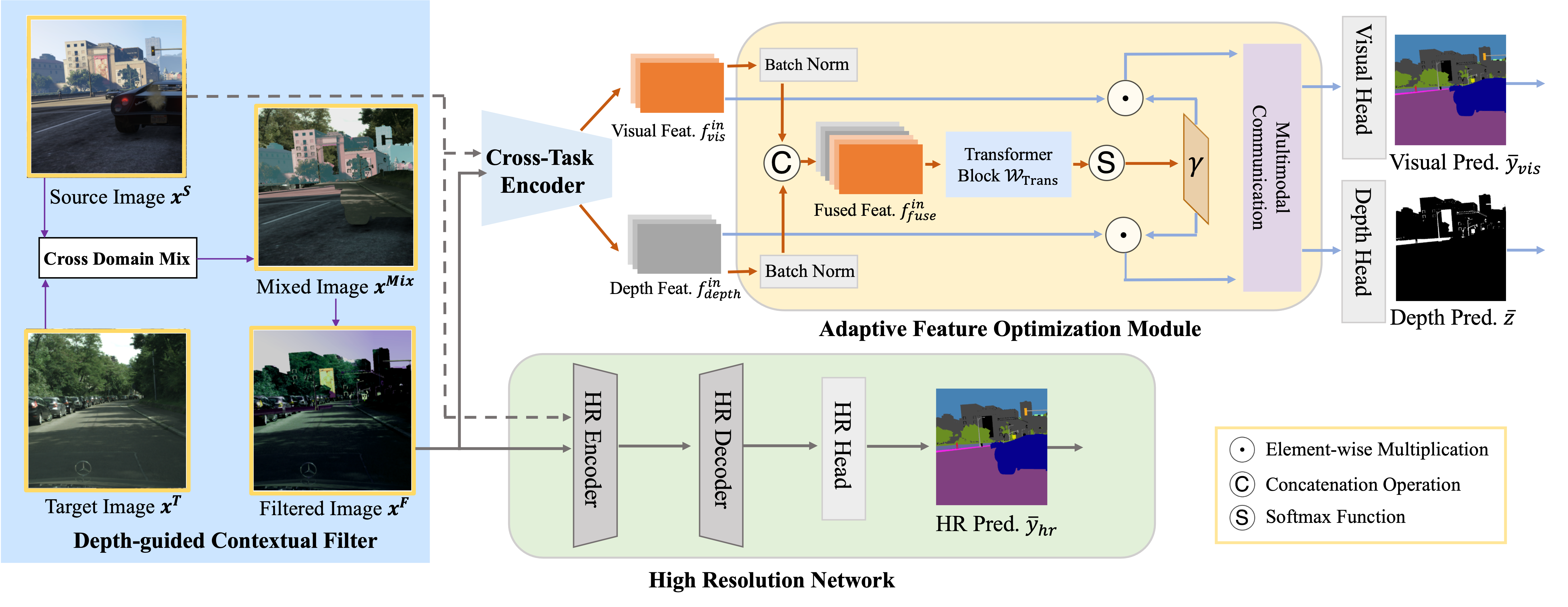
Figure 3: The proposed multi-task learning framework. The input images $x^{F}$ are mixed from the source image $x^{S}$ and target domain $x^{T}$ according to the depth (Please refer to Figure 2). Then we are fed $x^{S}$ and $x^{F}$ into the high resolution encoder to generate high resolution predictions. To enhance multi-modal learning, the visual and depth feature created by the cross-task encoder are fused and fed into the proposed Adaptive Feature Optimization module (AFO) for multimodal communication. Finally, the multimodal communication via several transformer blocks incorporates and optimizes the fusion of depth information, improving the final visual predictions.

3.2 Depth-guided Contextual Filter

In UDA, recent works [27, 21, 22, 23, 1, 25] apply the strategy to generate cross-domain augmented samples by mixing pixels. The typical mixing is to copy one set of pixels from a source domain image and paste such pixels to one set of pixels from a target domain image. Due to the different layouts between source and target domain data, it is challenging for such a vanilla method to craft high-quality cross-domain mixing samples for training. To decrease noisy signals and simulate augmented training samples with real-world layouts, we propose Depth-guided Contextual Filter to reduce the noisy pixels that are naively mixed across domains.

Based on the hypothesis that most semantic categories usually fall under a finite depth range, we introduce DCF, which divides the target depth map $\mathbf{z}^{T}$ into a few discrete depth intervals $(I_{z}1,...,I_{z}n)$. The implementation of DCF is represented as pseudo-code in Algorithm 1, where the image $\mathbf{x}^{S}$ and the corresponding semantic labels $\mathbf{y}^{S}$ are sampled from source domain data. The image $\mathbf{x}^{T}$ and the depth label $\mathbf{z}^{T}$ are from target domain data. Pseudo label $\hat{\mathbf{y}}^{T}$ is then generated:

$$\hat{\mathbf{y}}^{T}=\mathcal{F}_{\theta}\left(\mathbf{x}^{T}\right).$$ (1)

For a given real-world target input image $\mathbf{x}^{T}$ combined with the pseudo label $\hat{\mathbf{y}}^{T}$ and target depth map $\mathbf{z}^{T}$, the density value at each depth interval $(I_{z1},...,I_{zn})$ for each class $i\in(1,\ldots,C)$ can be pre-calculated. For example, the density value for class $i$ at the depth interval $I_{z1}$ is calculated as $p(i,I_{z1})$. All the density values make up the depth distribution in the target domain image. Then we randomly select half of the categories on the source images. In practice, we apply a binary mask $\mathcal{M}$ to denote the corresponding pixels. Then naive cross-domain mixed image $\mathbf{x}^{Mix}$ and the mixed label $\hat{\mathbf{y}}^{Mix}$ can be formulated as:

$$\mathbf{x}^{Mix}=\mathcal{M}\odot\mathbf{x}^{S}+\left(1-\mathcal{M}\right)\odot\mathbf{x}^{T},$$ (2)

$$\hat{\mathbf{y}}^{Mix}=\mathcal{M}\odot\mathbf{y}^{S}+\left(1-\mathcal{M}\right)\odot\hat{\mathbf{y}}^{T},$$ (3)

where $\odot$ denotes the element-wise multiplication of between the mask and the image. The naively mixed images are visualized in Figure 2. It could be observed that due to the depth distribution difference between two domains, pixels of “Building” category are mixed from the source domain to the target domain, creating unrealistic images. Training with such training samples will compromise contextual learning. Therefore, we propose to filter the pixels that do not match the depth density distribution in the mixed image. After the naive mixing, we re-calculate the density value for each class at each depth interval. For example, the new density value for class $i$ at the depth interval $I_{z1}$ is denoted as $\hat{p}\left(i,I_{z1}\right)$. Then we calculate the depth density distribution difference for each pasted category and denote the difference for class $i$ at the depth interval $I_{z1}$ as $\text{diff}^{z1}_{i}$. Once $\text{diff}^{z1}_{i}$ exceeds the threshold of that category $i$, these pasted pixels are removed. After performing DCF, we confirm the final realistic pixels to be mixed and construct a depth-aware binary mask $\mathcal{M^{DCF}}$, which is changed dynamically based on the depth layout of the current target image.

The filtered mixing samples are then generated. In practice, we directly apply the updated depth-aware mask to replace the original mask. Therefore, the new mixed sample and the label are as follows:

$$\mathbf{x}^{F}=\mathcal{M^{DCF}}\odot\mathbf{x}^{S}+\left(1-\mathcal{M^{DCF}}\right)\odot\mathbf{x}^{T},$$ (4)

$$\hat{\mathbf{y}}^{F}=\mathcal{M^{DCF}}\odot\mathbf{y}^{S}+\left(1-\mathcal{M^{DCF}}\right)\odot\hat{\mathbf{y}}^{T}.$$ (5)

The filtered samples could be visualized in Figure 2. Because large objects such as “sky” and “terrain” usually aggregate and occupy a large amount of pixels and small objects only occupy a small amount of pixels in a certain depth range, we set different filtering thresholds for each category. DCF uses pseudo semantic labels for the target domain as there is no ground truth available. Since the label prediction is not stable in the early stage, we apply a warmup strategy to perform DCF after 10000 iterations. Examples of the input images, naively mixed samples and filtered samples are presented in Figure 2. The sample after the process of the DCF module has the pixels from the source domain that match the depth distribution of the target domain, helping the network to better deal with the domain gap.

3.3 Multi-task Scene Adaptation Framework

In order to exploit the relation between segmentation and depth learning, we introduce a multi-task scene adaptation framework including a high resolution semantic encoder, and a cross-task shared encoder with a feature optimization module, which is depicted in Figure 3. The proposed framework incorporates and optimizes the fusion of depth information for improving the final semantic predictions.

High Resolution Semantic Prediction.

Most supervised methods use high resolution images for training, but common scene adaptation methods usually use random crops of the image that is half of the full resolution. To reduce the domain gap between scene adaptation and supervised learning while maintaining the GPU memory consumption, we adopt a high-resolution encoder to encode HR image crops into deep HR features. Then a semantic decoder is used to generate the HR semantic predictions $\bar{\mathbf{y}}_{hr}$. We adopt the cross entropy loss for semantic segmentation:

$${\mathcal{L}}_{hr}^{S}\left(\mathbf{x}^{S},\mathbf{y}^{S}\right) =\mathbb{E}\left[-\mathbf{y}^{S}\log\bar{\mathbf{y}}_{hr}^{S}\right],$$ (6)

$${\mathcal{L}}_{hr}^{F}\left(\mathbf{x}^{F},\mathbf{y}^{F}\right) =\mathbb{E}\left[-\hat{\mathbf{y}}^{F}\log\bar{\mathbf{y}}_{hr}^{F}\right],$$ (7)

where $\bar{\mathbf{y}}_{hr}^{S}$ and $\bar{\mathbf{y}}_{hr}^{T}$ are high resolution semantic predictions. $\mathbf{y}^{S}$ is the one-hot semantic label for the source domain and $\hat{\mathbf{y}}^{F}$ is the one-hot pseudo label for the depth-aware fused domain.

Adaptive Feature Optimization.

In addition to the high resolution encoder, We use another cross-task encoder to encode input images which are shared for both tasks. Depth maps are rich in spatial depth information, but a naive concatenation of depth information directly to visual information causes some interference, e.g. categories at similar depth positions are already well distinguished by visual information, and attention mechanisms can help the network to select the crucial part of the multitask information. In the proposed multi-task learning framework, the visual semantic feature and depth feature is generated by a visual head and a depth head, respectively. As shown in Figure 3, after applying batch normalization, an Adaptive Feature Optimization module then concatenates the normalized input visual feature and the input depth feature to create a fused multi-task feature:

Table 1: Quantitative comparison with previous UDA methods on GTA $\rightarrow$ Cityscapes. We present pre-class IoU and mIoU. The best accuracy in every column is in bold. Our results are averaged over 3 random seeds. Further methods are shown in the supplementary materials.

Method	Road	SW	Build	Wall	Fence	Pole	TL	TS	Veg.	Terrain	Sky	PR	Rider	Car	Truck	Bus	Train	Motor	Bike	mIoU
AdvEnt [28]	89.4	33.1	81.0	26.6	26.8	27.2	33.5	24.7	83.9	36.7	78.8	58.7	30.5	84.8	38.5	44.5	1.7	31.6	32.4	45.5
MRNet [35]	89.1	23.9	82.2	19.5	20.1	33.5	42.2	39.1	85.3	33.7	76.4	60.2	33.7	86.0	36.1	43.3	5.9	22.8	30.8	45.5
APODA [66]	85.6	32.8	79.0	29.5	25.5	26.8	34.6	19.9	83.7	40.6	77.9	59.2	28.3	84.6	34.6	49.2	8.0	32.6	39.6	45.9
CBST [15]	91.8	53.5	80.5	32.7	21.0	34.0	28.9	20.4	83.9	34.2	80.9	53.1	24.0	82.7	30.3	35.9	16.0	25.9	42.8	45.9
PatchAlign [67]	92.3	51.9	82.1	29.2	25.1	24.5	33.8	33.0	82.4	32.8	82.2	58.6	27.2	84.3	33.4	46.3	2.2	29.5	32.3	46.5
MRKLD [16]	91.0	55.4	80.0	33.7	21.4	37.3	32.9	24.5	85.0	34.1	80.8	57.7	24.6	84.1	27.8	30.1	26.9	26.0	42.3	47.1
BL [39]	91.0	44.7	84.2	34.6	27.6	30.2	36.0	36.0	85.0	43.6	83.0	58.6	31.6	83.3	35.3	49.7	3.3	28.8	35.6	48.5
DT [68]	90.6	44.7	84.8	34.3	28.7	31.6	35.0	37.6	84.7	43.3	85.3	57.0	31.5	83.8	42.6	48.5	1.9	30.4	39.0	49.2
Uncertainty [17]	90.4	31.2	85.1	36.9	25.6	37.5	48.8	48.5	85.3	34.8	81.1	64.4	36.8	86.3	34.9	52.2	1.7	29.0	44.6	50.3
DACS [20]	89.9	39.7	87.9	30.7	39.5	38.5	46.4	52.8	88.0	44.0	88.8	67.2	35.8	84.5	45.7	50.2	0.0	27.3	34.0	52.1
BAPA [69]	94.4	61.0	88.0	26.8	39.9	38.3	46.1	55.3	87.8	46.1	89.4	68.8	40.0	90.2	60.4	59.0	0.0	45.1	54.2	57.4
ProDA [36]	87.8	56.0	79.7	46.3	44.8	45.6	53.5	53.5	88.6	45.2	82.1	70.7	39.2	88.8	45.5	59.4	1.0	48.9	56.4	57.5
DAFormer [22]	95.7	70.2	89.4	53.5	48.1	49.6	55.8	59.4	89.9	47.9	92.5	72.2	44.7	92.3	74.5	78.2	65.1	55.9	61.8	68.3
CAMix [49]	96.0	73.1	89.5	53.9	50.8	51.7	58.7	64.9	90.0	51.2	92.2	71.8	44.0	92.8	78.7	82.3	70.9	54.1	64.3	70.0
HRDA [23]	96.4	74.4	91.0	61.6	51.5	57.1	63.9	69.3	91.3	48.4	94.2	79.0	52.9	93.9	84.1	85.7	75.9	63.9	67.5	73.8
MIC [1]	97.4	80.1	91.7	61.2	56.9	59.7	66.0	71.3	91.7	51.4	94.3	79.8	56.1	94.6	85.4	90.3	80.4	64.5	68.5	75.9
CorDA† [21]	94.7	63.1	87.6	30.7	40.6	40.2	47.8	51.6	87.6	47.0	89.7	66.7	35.9	90.2	48.9	57.5	0.0	39.8	56.0	56.6
FAFS† [70]	93.4	60.7	88.0	43.5	32.1	40.3	54.3	53.0	88.2	44.5	90.0	69.5	35.8	88.7	34.1	53.9	41.3	51.7	54.7	58.8
DBST† [70]	94.3	60.0	87.9	50.5	43.0	42.6	50.8	51.3	88.0	45.9	89.7	68.9	41.8	88.0	45.8	63.8	0.0	50.0	55.8	58.8
Ours†	97.5	80.7	92.1	66.4	62.3	63.1	67.7	75.7	91.8	52.4	93.9	81.6	61.8	94.7	88.3	90.0	81.2	65.8	69.6	77.7

^†: Training with depth data.

$$f_{fuse}^{in}=\operatorname{CONCAT}\left(f_{vis}^{in},f_{depth}^{in}\right),$$ (8)

where $\operatorname{CONCAT}\left(,\right)$ denotes the concatenation operation. The fused feature is then fed into a series of transformer blocks to capture the key information between the two tasks. The attention mechanism adaptively adjusts the extent to which depth features are embedded in visual features.

$$f_{fuse}^{out}=\mathcal{W}_{Trans}\left(f_{fuse}^{in}\right),$$ (9)

where $\mathcal{W}_{Trans}$ is the transformer parameter. The learned output of the transformer blocks is a weight map $\gamma$ which is multiplied back to the input visual feature and depth feature, resulting in an optimized feature for each task.

$$\bm{\gamma}=\bm{\sigma}\left(\mathcal{W}_{Conv}\otimes f_{fuse}^{out}\right),$$ (10)

where $\mathcal{W}_{Conv}$ denotes the convolution parameter, $\otimes$ denotes the convolution operation and $\bm{\sigma}$ represents the sigmoid function. The weight matrix $\bm{\gamma}$ performs adaptive optimization of the muti-task features. And then the fused feature $f_{fuse}^{out}$ is fed into different decoders for predicting different final tasks, i.e., the visual and the depth task. The output features are essentially multimodal features containing crucial depth information.

$$f_{vis}^{out}=f_{vis}^{out}\odot\bm{\gamma},$$ (11)

$$f_{depth}^{out}=f_{depth}^{out}\odot\bm{\gamma},$$ (12)

where $\odot$ represents element-wise multiplication. The optimized visual and depth feature is then fed into the multimodal communication module for further processing. The multimodal communication module refines the learning of key information between two tasks by iterative use of transformer blocks. the inference is merely based on the visual input when the feature optimization is fished. The final semantic prediction $\bar{\mathbf{y}}_{vis}^{S}$ and depth prediction $\bar{\mathbf{z}}^{S}$ can be generated from the final visual feature $f_{vis}^{final}$ and depth feature $f_{depth}^{final}$ by the visual head and depth head . Similar to the high resolution predictions, we use the cross entropy loss for the semantic loss calculation:

$${\mathcal{L}}_{vis}^{S}\left(\mathbf{x}^{S},\mathbf{y}^{S}\right)=\mathbb{E}\left[-\mathbf{y}^{S}\log\bar{\mathbf{y}}_{vis}^{S}\right],$$ (13)

$${\mathcal{L}}_{vis}^{F}\left(\mathbf{x}^{F},\mathbf{y}^{F}\right)=\mathbb{E}\left[-\hat{\mathbf{y}}^{F}\log\bar{\mathbf{y}}_{vis}^{F}\right].$$ (14)

We also employ the berHu loss for depth regression at source domain:

$${\mathcal{L}}_{depth}^{S}\left(\mathbf{z}^{S}\right)=\mathbb{E}\left[\operatorname{berHu}\left(\bar{\mathbf{z}}^{S}-\mathbf{z}^{S}\right)\right],$$ (15)

where $\bar{z}$ and $z$ are predicted and ground truth semantic maps. Following [61, 63], we deploy the reversed Huber criterion [71], which is defined as :

$$\operatorname{ber}Hu\left(e_{z}\right) =\left\{\begin{array}[]{cc}\left|e_{z}\right|,&\left|e_{z}\right|\leq H\\ \frac{\left(e_{z}\right)^{2}+H^{2}}{2H},&\left|e_{z}\right|>H\end{array}\right.$$ (16)

$$H =0.2\max\left(\left|e_{z}\right|\right),$$

where $H$ is a positive threshold and we set it to $0.2$ of the maximum depth residual. Finally, the overall loss function is:

$${\mathcal{L}}={\mathcal{L}}_{hr}^{S}+{\mathcal{L}}_{vis}^{S}+\lambda_{depth}{\mathcal{L}}_{depth}^{S}+{\mathcal{L}}_{hr}^{F}+{\mathcal{L}}_{vis}^{F},$$ (17)

where hyperparameter $\lambda_{depth}$ is the loss weight. Considering that our main task is semantic segmentation and the depth estimation is the auxiliary task, we empirically $\lambda_{depth}=0.1\times 10^{-2}$. We also designed the ablation studies to change the weight of depth task $\lambda_{depth}$ to the level of $10^{-1}$ or $10^{-3}$.

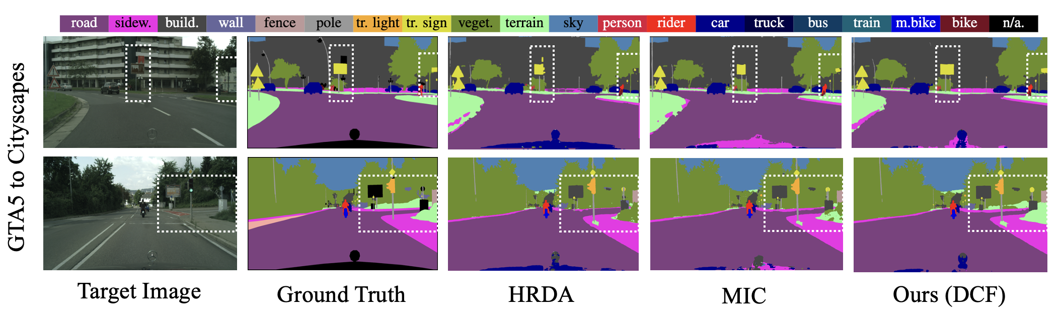
Figure 4: Qualitative results on GTA $\rightarrow$ Cityscapes. From left to right: Target Image, Ground Truth, the visual results predicted by HRDA, MIC and Ours. We deploy the white dash boxes to highlight different prediction parts. The proposed method could predict clear edges. More examples are shown in the supplementary materials.

4 Experiment

4.1 Implementation Details

Datasets.

We evaluate the proposed framework on two scene adaptation settings, i.e., GTA $\rightarrow$ Cityscapes and SYNTHIA $\rightarrow$ Cityscapes, following common protocols [20, 21, 46, 22, 23, 1]. Particularly, the GTA5 dataset [8] is the synthetic dataset collected from a video game, which contains 24,966 images annotated by 19 classes. Following [21], we adopt depth information generated by Monodepth2 [65] model which is trained merely on GTA image sequences. SYNTHIA [9] is a synthetic urban scene dataset with 9,400 training images and 16 classes. Simulated depth information provided by SYNTHIA is used. GTA and SYNTHIA serve as source domain datasets. The target domain dataset is Cityscapes, which is collected from real-world street-view images. Cityscapes contains 2,975 unlabeled training images and 500 validation images. The resolution of Cityscapes is 2048 $\times$ 1024 and the common protocol downscales the size to 1024 $\times$ 512 to save memory. Following [21], the stereo depth estimation from [72] is used. We leverage the Intersection Over Union (IoU) for per-class performance and the mean Intersection over Union (mIoU) over all classes to report the result. The code is based on Pytorch [73]. We will make our code open-source for reproducing all results.

Experimental Setup.

We adopt DAFormer [22] network with MiT-B5 backbone [5] for the high resolution encoder and DeepLabV2 network with ResNet-101 backbone for the cross-task encoder to reduce the memory consumption. All backbones are initialized with ImageNet pretraining. Our training procedure is based on self-training methods with cross-domain mixing [20, 22, 23, 1] and enhanced by our proposed Depth-guided Contextual Filter. Following [20, 23], the input image resolution is half of the full resolution for the cross-task encoder and full resolution for high resolution encoder. We utilize the same data augmentation e.g., color jitter and Gaussian blur and empirically set pseudo labels threshold $0.968$ following [20]. We train the network with batch size 2 for 40k iterations on a Tesla V100 GPU.

4.2 Comparison with SOTA

Table 2: Quantitative comparison with previous UDA methods on SYNTHIA $\rightarrow$ Cityscapes. We present pre-class IoU and mIoU. mIoU are averaged over 16 categories, respectively. The best accuracy in every column is in bold. Our results are averaged over 3 random seeds. Further methods are shown in the supplementary materials.

Method	Road	SW	Build	Wall*	Fence*	Pole*	TL	TS	Veg.	Sky	PR	Rider	Car	Bus	Motor	Bike	mIoU
MaxSquare [43]	77.4	34.0	78.7	5.6	0.2	27.7	5.8	9.8	80.7	83.2	58.5	20.5	74.1	32.1	11.0	29.9	39.3
AdaptSegNet [12]	84.3	42.7	77.5	$-$	$-$	$-$	4.7	7.0	77.9	82.5	54.3	21.0	72.3	32.2	18.9	32.3	46.7
AdvEnt [28]	85.6	42.2	79.7	8.7	0.4	25.9	5.4	8.1	80.4	84.1	57.9	23.8	73.3	36.4	14.2	33.0	41.2
ASA [74]	91.2	48.5	80.4	3.7	0.3	21.7	5.5	5.2	79.5	83.6	56.4	21.0	80.3	36.2	20.0	32.9	41.7
CBST [15]	68.0	29.9	76.3	10.8	1.4	33.9	22.8	29.5	77.6	78.3	60.6	28.3	81.6	23.5	18.8	39.8	42.6
CLAN [13]	81.3	37.0	80.1	$-$	$-$	$-$	16.1	13.7	78.2	81.5	53.4	21.2	73.0	32.9	22.6	30.7	47.8
SP-Adv [75]	84.8	35.8	78.6	$-$	$-$	$-$	6.2	15.6	80.5	82.0	66.5	22.7	74.3	34.1	19.2	27.3	48.3
Uncertainty [17]	87.6	41.9	83.1	14.7	1.7	36.2	31.3	19.9	81.6	80.6	63.0	21.8	86.2	40.7	23.6	53.1	47.9
APODA [66]	86.4	41.3	79.3	$-$	$-$	$-$	22.6	17.3	80.3	81.6	56.9	21.0	84.1	49.1	24.6	45.7	53.1
IAST [76]	81.9	41.5	83.3	17.7	4.6	32.3	30.9	28.8	83.4	85.0	65.5	30.8	86.5	38.2	33.1	52.7	49.8
DAFormer [22]	84.5	40.7	88.4	41.5	6.5	50.0	55.0	54.6	86.0	89.8	73.2	48.2	87.2	53.2	53.9	61.7	60.9
HRDA [23]	85.2	47.7	88.8	49.5	4.8	57.2	65.7	60.9	85.3	92.9	79.4	52.8	89.0	64.7	63.9	64.9	65.8
MIC [1]	86.6	50.5	89.3	47.9	7.8	59.4	66.7	63.4	87.1	94.6	81.0	58.9	90.1	61.9	67.1	64.3	67.3
DADA† [61]	89.2	44.8	81.4	6.8	0.3	26.2	8.6	11.1	81.8	84.0	54.7	19.3	79.7	40.7	14.0	38.8	42.6
CorDA† [21]	93.3	61.6	85.3	19.6	5.1	37.8	36.6	42.8	84.9	90.4	69.7	41.8	85.6	38.4	32.6	53.9	55.0
Ours†	93.4	63.1	89.8	51.1	9.1	61.4	66.9	64.0	88.0	94.5	80.9	56.6	90.9	68.5	63.7	66.6	69.3

^†: Training with depth data.

Table 3: Ablation study of different components of our proposed framework on GTA$\rightarrow$Cityscapes. The results are averaged over 3 random seeds.

Method	ST Base.	Naive Mix.	DCF.	AFO. (CA)	AFO. (Trans + MMC)	mIoU$\uparrow$
M1	$\checkmark$					$73.1$
M2	$\checkmark$	$\checkmark$				$76.0$
M3	$\checkmark$	$\checkmark$	$\checkmark$			$77.1$
M4	$\checkmark$	$\checkmark$	$\checkmark$	$\checkmark$		$77.3$
M5	$\checkmark$	$\checkmark$	$\checkmark$		$\checkmark$	$77.7$

Table 4: Compatibility of the proposed method on different UDA methods and backbones on GTA$\rightarrow$Cityscapes. Our results are averaged over 3 random seeds.

Backbone	UDA Method	w/o	w/	Diff.
DeepLabV2 [2]	DACS [20]	$52.1$	$56.2$	$+4.1$
DAFormer [22]	DAFormer [22]	$68.3$	$71.5$	$+3.2$
DAFormer [22]	HRDA [23]	$73.8$	$76.1$	$+2.3$
DAFormer [22]	MIC [1]	$75.9$	$77.7$	$+1.8$

Results on GTA$\rightarrow$Cityscapes.

We show our results on GTA $\rightarrow$ Cityscapes in Table 1 and highlight the best results in bold. It could be observed that our method yields significant performance improvement over the state-of-the-art method MIC [1] from 75.9 mIoU to 77.7 mIoU. Usually, classes that occupy a small number of pixels are difficult to adapt and have a comparably low IoU performance. However, our method demonstrates competitive IoU improvement on most categories especially on small objects such as +5.7 on “Rider”, +5.4 on “Fence”, +5.2 on “Wall”, +4.4 on “Traffic Sign” and +3.4 on “Pole”. The result shows the effectiveness of the proposed contextual filter and cross-task learning framework in the contextual learning. Our method also increases the mIoU performance of classes that aggregate and occupy a large amount of pixels in an image by a smaller margi such as +1.8 on “Pedestrain” and +1.1 on “Bike”, probably because the rich texture and color information contained in the visual feature already has the ability to recognize these relatively easier classes. The above observations are also qualitatively reflected in Figure 4, where we visualize the segmentation results of the proposed method and the comparison with previous strong transformer-based methods HRDA [23], and MIC [1]. The qualitative results highlighted by white dash boxes show that the proposed method largely improved the prediction quality of challenging small object “Traffic Sign” and large category “Terrain”.

Results on Synthia$\rightarrow$Cityscapes.

We show our results on SYNTHIA $\rightarrow$ Cityscapes in Table 1 and the results show the consistent performance improvement of our method, increasing from 67.3 to 69.3 (+2.0 mIoU) compared to the state-of-the-art method MIC [1]. Especially, our method significantly increases the IoU performance of the challenging class “SideWalk” from 50.5 to 63.1 (+12.6 mIoU). It is also noticeable that our method remains competitive in segmenting most individual classes and yields a significant increase of +6.8 on “Road”, +6.6 on “Bus”, +3.9 on “Pole” +3.7 on “Road”, +3.2 on “Wall” and +2.9 on “Truck”.

4.3 Ablation Study on Different Scene Adaptation Frameworks

We combine our method with different scene adaptation architectures on GTA$\rightarrow$Cityscapes. Table 4 shows that our method achieves consistent and significant improvements across different methods with different network architectures. Firstly, our method improves the state-of-the-art performance by +1.8 mIoU. Then we evaluate the proposed method on two strong methods based on transformer backbone, yielding +3.2 mIoU and +2.3 mIoU performance increase on DAFormer [22] and HRDA [23], respectively. Secondly, we evaluate our method on DeepLabV2 [2] architecture with ResNet-101 [77] backbone. We show that we improve the performance of the CNN-based cross-domain mixing method, i.e., DACS by +4.1 mIoU. The ablation study verifies the effectiveness of our method in leveraging depth information to enhance cross-domain mixing not only on Transformer-based networks but also on CNN-based architecture.

4.4 Ablation Study on Different Components of the Proposed Method

In order to verify the effectiveness of our proposed components, we train four different models from M1 to M4 and show the result in Table 3. “ST Base” means the self training baseline with semantic segmentation branch and depth regression branch. “Naive Mix” denotes the cross-domain mixing strategy. “DCF” represents the proposed depth-aware mixing (Depth-guided Contextual Filter). “AFO” denotes the proposed Adaptive Feature Optimization module and we used two different method to perform AFO. Firstly, we leverage channel attention (CA) that could select useful information along the channel dimension to perform the feature optimization. In this method, the fused feature is adaptively optimized by SENet [78], the output is a weighted vector which is multiplied back to the visual and depth feature. We use “AFO (CA)” to denote this method. Secondly, we leverage the iterative use of transformer block to adaptively optimize the multi-task feature. In this case, the output of the transformer block is a weighted map. The Multimodal Communication (MMC) module is then used to incorporate rich knowledge from the depth prediction. We denote this method as “AFO (Trans + MMC)”. M1 is the self training baseline with depth regression based on DAFormer architecture. M2 adds the cross-domain mixing strategy for improvement and shows a competitive result of 76.0 mIoU. M3 is the model with the Depth-guided Contextual Filter, increasing the performance from 76.0 to 77.1 mIoU (+1.1 mIoU), which demonstrates the effectiveness of transferring the mixed training images to real-world layout with the help of the depth information. M4 adds the multi-task framework that leverages Channel Attention (CA) mechanism to fuse the discriminative depth feature into the visual feature. The segmentation result is increased by a small margin (+0.2 mIoU), which means CA could help the network to adaptively learn to focus or to ignore information from the auxiliary task to some extent. M5 is our proposed depth-aware multi-task model with both Depth-guided Contextual Filter and Adaptive Feature Optimization (AFO) module. Compared to M3, M5 has a mIoU increase of +0.6 from 77.1 to 77.7, which shows the effectiveness of multi-modal feature optimization using transformers to facilitate contextual learning.

5 Conclusion

In this work, we introduce a new depth-aware scene adaptation framework that effectively leverages the guidance of depth to enhance data augmentation and contextual learning. The proposed framework not only explicitly refines the cross-domain mixing by stimulating real-world layouts with the guidance of depth distributions of objects, but also introduced a cross-task encoder that adaptively optimizes the multi-task feature and focused on the discriminative depth feature to help contextual learning. By integrating our depth-aware framework into existing self-training methods based on either transformer or CNN, we achieve state-of-the-art performance on two widely used benchmarks and a significant improvement on small-scale categories. Extensive experimental results verify our motivation to transfer the training images to real-world layouts and demonstrate the effectiveness of our multi-task framework in improving scene adaptation performance.

References

- [1] Lukas Hoyer, Dengxin Dai, Haoran Wang, and Luc Van Gool. MIC: Masked image consistency for context-enhanced domain adaptation. In CVPR, 2023.
- [2] Liang-Chieh Chen, George Papandreou, Iasonas Kokkinos, Kevin Murphy, and Alan L Yuille. Deeplab: Semantic image segmentation with deep convolutional nets, atrous convolution, and fully connected crfs. IEEE transactions on pattern analysis and machine intelligence, 40(4):834–848, 2017.
- [3] Jonathan Long, Evan Shelhamer, and Trevor Darrell. Fully convolutional networks for semantic segmentation. In CVPR, 2015.
- [4] Vijay Badrinarayanan, Alex Kendall, and Roberto Cipolla. Segnet: A deep convolutional encoder-decoder architecture for image segmentation. IEEE transactions on pattern analysis and machine intelligence, 39(12):2481–2495, 2017.
- [5] Enze Xie, Wenhai Wang, Zhiding Yu, Anima Anandkumar, Jose M Alvarez, and Ping Luo. Segformer: Simple and efficient design for semantic segmentation with transformers. NeurIPS, 2021.
- [6] Bolei Zhou, Hang Zhao, Xavier Puig, Tete Xiao, Sanja Fidler, Adela Barriuso, and Antonio Torralba. Semantic understanding of scenes through the ade20k dataset. International Journal of Computer Vision, 127:302–321, 2019.
- [7] Marius Cordts, Mohamed Omran, Sebastian Ramos, Timo Rehfeld, Markus Enzweiler, Rodrigo Benenson, Uwe Franke, Stefan Roth, and Bernt Schiele. The cityscapes dataset for semantic urban scene understanding. In CVPR, 2016.
- [8] Stephan R Richter, Vibhav Vineet, Stefan Roth, and Vladlen Koltun. Playing for data: Ground truth from computer games. In ECCV, 2016.
- [9] German Ros, Laura Sellart, Joanna Materzynska, David Vazquez, and Antonio M Lopez. The synthia dataset: A large collection of synthetic images for semantic segmentation of urban scenes. In CVPR, 2016.
- [10] Judy Hoffman, Eric Tzeng, Taesung Park, Jun-Yan Zhu, Phillip Isola, Kate Saenko, Alexei Efros, and Trevor Darrell. Cycada: Cycle-consistent adversarial domain adaptation. In ICML, 2018.
- [11] Zuxuan Wu, Xin Wang, Joseph E Gonzalez, Tom Goldstein, and Larry S Davis. Ace: Adapting to changing environments for semantic segmentation. In ICCV, 2019.
- [12] Yi-Hsuan Tsai, Wei-Chih Hung, Samuel Schulter, Kihyuk Sohn, Ming-Hsuan Yang, and Manmohan Chandraker. Learning to adapt structured output space for semantic segmentation. In CVPR, 2018.
- [13] Yawei Luo, Liang Zheng, Tao Guan, Junqing Yu, and Yi Yang. Taking a closer look at domain shift: Category-level adversaries for semantics consistent domain adaptation. In CVPR, 2019.
- [14] Harsh Rangwani, Sumukh K Aithal, Mayank Mishra, Arihant Jain, and Venkatesh Babu Radhakrishnan. A closer look at smoothness in domain adversarial training. In ICML, 2022.
- [15] Yang Zou, Zhiding Yu, BVK Kumar, and Jinsong Wang. Unsupervised domain adaptation for semantic segmentation via class-balanced self-training. In ECCV, 2018.
- [16] Yang Zou, Zhiding Yu, Xiaofeng Liu, BVK Kumar, and Jinsong Wang. Confidence regularized self-training. In ICCV, 2019.
- [17] Zhedong Zheng and Yi Yang. Rectifying pseudo label learning via uncertainty estimation for domain adaptive semantic segmentation. International Journal of Computer Vision, 129(4):1106–1120, 2021.
- [18] Yanchao Yang and Stefano Soatto. Fda: Fourier domain adaptation for semantic segmentation. In CVPR, 2020.
- [19] Ruihuang Li, Shuai Li, Chenhang He, Yabin Zhang, Xu Jia, and Lei Zhang. Class-balanced pixel-level self-labeling for domain adaptive semantic segmentation. In CVPR, 2022.
- [20] Wilhelm Tranheden, Viktor Olsson, Juliano Pinto, and Lennart Svensson. Dacs: Domain adaptation via cross-domain mixed sampling. In WACV Workshop, 2021.
- [21] Qin Wang, Dengxin Dai, Lukas Hoyer, Luc Van Gool, and Olga Fink. Domain adaptive semantic segmentation with self-supervised depth estimation. In ICCV, 2021.
- [22] Lukas Hoyer, Dengxin Dai, and Luc Van Gool. Daformer: Improving network architectures and training strategies for domain-adaptive semantic segmentation. In CVPR, 2022.
- [23] Lukas Hoyer, Dengxin Dai, and Luc Van Gool. Hrda: Context-aware high-resolution domain-adaptive semantic segmentation. In ECCV, 2022.
- [24] Binhui Xie, Shuang Li, Mingjia Li, Chi Harold Liu, Gao Huang, and Guoren Wang. Sepico: Semantic-guided pixel contrast for domain adaptive semantic segmentation. arXiv:2204.08808, 2022.
- [25] Mu Chen, Zhedong Zheng, Yi Yang, and Tat-Seng Chua. Pipa: Pixel-and patch-wise self-supervised learning for domain adaptative semantic segmentation. arXiv:2211.07609, 2022.
- [26] Zhengkai Jiang, Yuxi Li, Ceyuan Yang, Peng Gao, Yabiao Wang, Ying Tai, and Chengjie Wang. Prototypical contrast adaptation for domain adaptive segmentation. In ECCV, 2022.
- [27] Viktor Olsson, Wilhelm Tranheden, Juliano Pinto, and Lennart Svensson. Classmix: Segmentation-based data augmentation for semi-supervised learning. In WACV, 2021.
- [28] Tuan-Hung Vu, Himalaya Jain, Maxime Bucher, Matthieu Cord, and Patrick Pérez. Advent: Adversarial entropy minimization for domain adaptation in semantic segmentation. In CVPR, 2019.
- [29] Lin Chen, Huaian Chen, Zhixiang Wei, Xin Jin, Xiao Tan, Yi Jin, and Enhong Chen. Reusing the task-specific classifier as a discriminator: Discriminator-free adversarial domain adaptation. In CVPR, 2022.
- [30] Xiangyu Yue, Yang Zhang, Sicheng Zhao, Alberto Sangiovanni-Vincentelli, Kurt Keutzer, and Boqing Gong. Domain randomization and pyramid consistency: Simulation-to-real generalization without accessing target domain data. In ICCV, 2019.
- [31] Yuyang Zhao, Zhun Zhong, Zhiming Luo, Gim Hee Lee, and Nicu Sebe. Source-free open compound domain adaptation in semantic segmentation. IEEE Transactions on Circuits and Systems for Video Technology, 32(10):7019–7032, 2022.
- [32] Xinyu Zhang, Dongdong Li, Zhigang Wang, Jian Wang, Errui Ding, Javen Qinfeng Shi, Zhaoxiang Zhang, and Jingdong Wang. Implicit sample extension for unsupervised person re-identification. In CVPR, 2022.
- [33] Hao Feng, Minghao Chen, Jinming Hu, Dong Shen, Haifeng Liu, and Deng Cai. Complementary pseudo labels for unsupervised domain adaptation on person re-identification. IEEE Transactions on Image Processing, 30:2898–2907, 2021.
- [34] Qing Lian, Fengmao Lv, Lixin Duan, and Boqing Gong. Constructing self-motivated pyramid curriculums for cross-domain semantic segmentation: A non-adversarial approach. In ICCV, 2019.
- [35] Zhedong Zheng and Yi Yang. Unsupervised scene adaptation with memory regularization in vivo. In IJCAI, 2020.
- [36] Pan Zhang, Bo Zhang, Ting Zhang, Dong Chen, Yong Wang, and Fang Wen. Prototypical pseudo label denoising and target structure learning for domain adaptive semantic segmentation. In CVPR, 2021.
- [37] Qiming Zhang, Jing Zhang, Wei Liu, and Dacheng Tao. Category anchor-guided unsupervised domain adaptation for semantic segmentation. In NeurIPS, 2019.
- [38] Myeongjin Kim and Hyeran Byun. Learning texture invariant representation for domain adaptation of semantic segmentation. In CVPR, 2020.
- [39] Yunsheng Li, Lu Yuan, and Nuno Vasconcelos. Bidirectional learning for domain adaptation of semantic segmentation. In CVPR, 2019.
- [40] Haoran Wang, Tong Shen, Wei Zhang, Ling-Yu Duan, and Tao Mei. Classes matter: A fine-grained adversarial approach to cross-domain semantic segmentation. In ECCV, 2020.
- [41] Lin Chen, Zhixiang Wei, Xin Jin, Huaian Chen, Miao Zheng, Kai Chen, and Yi Jin. Deliberated domain bridging for domain adaptive semantic segmentation. In NeurIPS, 2022.
- [42] Yahao Liu, Jinhong Deng, Jiale Tao, Tong Chu, Lixin Duan, and Wen Li. Undoing the damage of label shift for cross-domain semantic segmentation. In CVPR, 2022.
- [43] Minghao Chen, Hongyang Xue, and Deng Cai. Domain adaptation for semantic segmentation with maximum squares loss. In ICCV, 2019.
- [44] Shaohua Guo, Qianyu Zhou, Ye Zhou, Qiqi Gu, Junshu Tang, Zhengyang Feng, and Lizhuang Ma. Label-free regional consistency for image-to-image translation. In ICME, 2021.
- [45] Jinyu Yang, Weizhi An, Sheng Wang, Xinliang Zhu, Chaochao Yan, and Junzhou Huang. Label-driven reconstruction for domain adaptation in semantic segmentation. In ECCV, 2020.
- [46] Nikita Araslanov and Stefan Roth. Self-supervised augmentation consistency for adapting semantic segmentation. In CVPR, 2021.
- [47] Jaehoon Choi, Taekyung Kim, and Changick Kim. Self-ensembling with gan-based data augmentation for domain adaptation in semantic segmentation. In ICCV, 2019.
- [48] Luke Melas-Kyriazi and Arjun K Manrai. Pixmatch: Unsupervised domain adaptation via pixelwise consistency training. In CVPR, 2021.
- [49] Qianyu Zhou, Zhengyang Feng, Qiqi Gu, Jiangmiao Pang, Guangliang Cheng, Xuequan Lu, Jianping Shi, and Lizhuang Ma. Context-aware mixup for domain adaptive semantic segmentation. IEEE Transactions on Circuits and Systems for Video Technology, 2022.
- [50] Behnam Gholami, Pritish Sahu, Ognjen Rudovic, Konstantinos Bousmalis, and Vladimir Pavlovic. Unsupervised multi-target domain adaptation: An information theoretic approach. IEEE Transactions on Image Processing, 29:3993–4002, 2020.
- [51] Antoine Saporta, Tuan-Hung Vu, Matthieu Cord, and Patrick Pérez. Multi-target adversarial frameworks for domain adaptation in semantic segmentation. In ICCV, 2021.
- [52] Seunghun Lee, Wonhyeok Choi, Changjae Kim, Minwoo Choi, and Sunghoon Im. Adas: A direct adaptation strategy for multi-target domain adaptive semantic segmentation. In CVPR, 2022.
- [53] Zhenyu Zhang, Zhen Cui, Chunyan Xu, Zequn Jie, Xiang Li, and Jian Yang. Joint task-recursive learning for semantic segmentation and depth estimation. In ECCV, 2018.
- [54] Dan Xu, Wanli Ouyang, Xiaogang Wang, and Nicu Sebe. Pad-net: Multi-tasks guided prediction-and-distillation network for simultaneous depth estimation and scene parsing. In CVPR, 2018.
- [55] Menelaos Kanakis, David Bruggemann, Suman Saha, Stamatios Georgoulis, Anton Obukhov, and Luc Van Gool. Reparameterizing convolutions for incremental multi-task learning without task interference. In ECCV, 2020.
- [56] Simon Vandenhende, Stamatios Georgoulis, and Luc Van Gool. Mti-net: Multi-scale task interaction networks for multi-task learning. In ECCV, 2020.
- [57] Trevor Standley, Amir Zamir, Dawn Chen, Leonidas Guibas, Jitendra Malik, and Silvio Savarese. Which tasks should be learned together in multi-task learning? In ICML, 2020.
- [58] Zhenyu Zhang, Zhen Cui, Chunyan Xu, Yan Yan, Nicu Sebe, and Jian Yang. Pattern-affinitive propagation across depth, surface normal and semantic segmentation. In CVPR, 2019.
- [59] Yaxiong Wang, Yunchao Wei, Xueming Qian, Li Zhu, and Yi Yang. Ainet: Association implantation for superpixel segmentation. In 2021 IEEE/CVF International Conference on Computer Vision, ICCV 2021, Montreal, QC, Canada, October 10-17, 2021, pages 7058–7067. IEEE, 2021.
- [60] Kuan-Hui Lee, German Ros, Jie Li, and Adrien Gaidon. Spigan: Privileged adversarial learning from simulation. arXiv:1810.03756, 2018.
- [61] Tuan-Hung Vu, Himalaya Jain, Maxime Bucher, Matthieu Cord, and Patrick Pérez. Dada: Depth-aware domain adaptation in semantic segmentation. In ICCV, 2019.
- [62] Yuhua Chen, Wen Li, Xiaoran Chen, and Luc Van Gool. Learning semantic segmentation from synthetic data: A geometrically guided input-output adaptation approach. In CVPR, 2019.
- [63] Suman Saha, Anton Obukhov, Danda Pani Paudel, Menelaos Kanakis, Yuhua Chen, Stamatios Georgoulis, and Luc Van Gool. Learning to relate depth and semantics for unsupervised domain adaptation. In CVPR, 2021.
- [64] Quanliang Wu and Huajun Liu. Unsupervised domain adaptation for semantic segmentation using depth distribution. In NeurIPS, 2022.
- [65] Clément Godard, Oisin Mac Aodha, Michael Firman, and Gabriel J Brostow. Digging into self-supervised monocular depth estimation. In ICCV, 2019.
- [66] Jihan Yang, Ruijia Xu, Ruiyu Li, Xiaojuan Qi, Xiaoyong Shen, Guanbin Li, and Liang Lin. An adversarial perturbation oriented domain adaptation approach for semantic segmentation. In AAAI, 2020.
- [67] Yi-Hsuan Tsai, Kihyuk Sohn, Samuel Schulter, and Manmohan Chandraker. Domain adaptation for structured output via discriminative patch representations. In ICCV, 2019.
- [68] Zhonghao Wang, Mo Yu, Yunchao Wei, Rogerio Feris, Jinjun Xiong, Wen-mei Hwu, Thomas S Huang, and Honghui Shi. Differential treatment for stuff and things: A simple unsupervised domain adaptation method for semantic segmentation. In CVPR, 2020.
- [69] Yahao Liu, Jinhong Deng, Xinchen Gao, Wen Li, and Lixin Duan. Bapa-net: Boundary adaptation and prototype alignment for cross-domain semantic segmentation. In ICCV, 2021.
- [70] Adriano Cardace, Luca De Luigi, Pierluigi Zama Ramirez, Samuele Salti, and Luigi Di Stefano. Plugging self-supervised monocular depth into unsupervised domain adaptation for semantic segmentation. In CVPR, 2022.
- [71] Iro Laina, Christian Rupprecht, Vasileios Belagiannis, Federico Tombari, and Nassir Navab. Deeper depth prediction with fully convolutional residual networks. In 3DV, 2016.
- [72] Christos Sakaridis, Dengxin Dai, Simon Hecker, and Luc Van Gool. Model adaptation with synthetic and real data for semantic dense foggy scene understanding. In ECCV, 2018.
- [73] Adam Paszke, Sam Gross, Soumith Chintala, Gregory Chanan, Edward Yang, Zachary DeVito, Zeming Lin, Alban Desmaison, Luca Antiga, and Adam Lerer. Automatic differentiation in pytorch. 2017.
- [74] Wei Zhou, Yukang Wang, Jiajia Chu, Jiehua Yang, Xiang Bai, and Yongchao Xu. Affinity space adaptation for semantic segmentation across domains. IEEE Transactions on Image Processing, 30:2549–2561, 2020.
- [75] Yuhu Shan, Chee Meng Chew, and Wen Feng Lu. Semantic-aware short path adversarial training for cross-domain semantic segmentation. Neurocomputing, 380:125–132, 2020.
- [76] Ke Mei, Chuang Zhu, Jiaqi Zou, and Shanghang Zhang. Instance adaptive self-training for unsupervised domain adaptation. In ECCV, 2020.
- [77] Kaiming He, Xiangyu Zhang, Shaoqing Ren, and Jian Sun. Deep residual learning for image recognition. In CVPR, 2016.
- [78] Jie Hu, Li Shen, and Gang Sun. Squeeze-and-excitation networks. In CVPR, 2018.