Error Estimates for Finite Element Approximations of Viscoelastic Dynamics: The Generalized Maxwell Model

Abstract

We prove error estimates for a finite element approximation of viscoelastic dynamics based on continuous Galerkin in space and time, both in energy norm and in $L^{2}$ norm. The proof is based on an error representation formula using a discrete dual problem and a stability estimate involving the kinetic, elastic, and viscoelastic energies. To set up the dual error analysis and to prove the basic stability estimates, it is natural to formulate the problem as a system involving evolution equations for the viscoelastic stress, the displacements, and the velocities. The equations for the viscoelastic stress can, however, be solved analytically in terms of the deviatoric strain velocity, and therefore, the viscoelastic stress can be eliminated from the system, resulting in a system for displacements and velocities.

1 Introduction

For many industrial engineering applications, particularly designing mechanical structures with polymeric materials, accurate dynamic simulation of time-dependent materials is necessary for reliable results. Assuming small strains, the mechanical properties of time-dependent materials are well described by linear viscoelastic theory [17], and there exist several models for the constitutive equations of linear viscoelastic materials [3]. Based on various viscoelastic models formulated in the time or frequency domain, finite element methods incorporating viscoelastic dynamics have been developed, e.g., [4, 9, 7, 8, 6, 16, 11].

In this paper, we derive a priori error estimates for a space-time finite element method for the dynamic simulation of viscoelastic materials modeled using the generalized Maxwell model, also known as the Wiechert model. While there seems to exist quite a few papers regarding the a priori error analysis for quasi-static viscoelastic problems, e.g., [14, 13, 15, 10, 12], we have found only a few examples of a priori error estimates for finite element methods regarding dynamic viscoelasticity for this model. Campo et al. [1] proves an error estimate for a dynamic viscoelastic problem, but the analysis is limited to an explicit forward Euler-type scheme in time. A more rigorous analysis is performed by Rivière et al. [11] where a Crank–Nicolson type scheme in time and a nonsymmetric discontinuous Galerkin (dG) method in space are used. Recently, a more refined analysis was provided by Jang and Shaw [5] where a symmetric dG formulation in space was considered. This method and analysis share several nice features with the present work, such as error bounds that are only linear with respect to the end time $T$, error bounds also in terms of the $L^{2}$-error, and representing the viscoelastic stresses compactly using internal vector-valued variables.

Contributions.

In this work, we present and analyze a finite element method for the dynamical simulation of linear viscoelastic materials modeled using the generalized Maxwell model. The method is based on approximation spaces that are continuous piecewise linear in time and continuous piecewise polynomial of order $p$ in space. In summary, our main contributions are:

• We prove space-time a priori error estimates in the end time energy norm and in the end time $L^{2}$ norm of the displacement field. The proofs of both estimates are based on the same error representation formula derived using a discrete dual problem, which provides a framework that can be used to analyze a wide range of methods.

• By avoiding arguments involving Grönwall’s lemma, our error estimates only linearly depend on the end time $T$, rather than exponentially as is the case when using Grönwall style arguments [11]. This property is shared with the analysis in [5].

• The viscoelastic components of the stresses are, as in [5], compactly modeled using vector-valued internal variables. In addition, we demonstrate how these internal variables can be eliminated from the system of equations in each time step. This leads to a greatly reduced system with only displacements and velocities as unknowns, where the internal variables at the next time are readily reconstructed using a simple formula.

• In our analysis, the viscoelastic components of the stress are formulated in terms of a different differential operator than the elastic stress, the deviatoric strain, leading to a more involved analysis. In practice, viscoelastic stresses are often modeled using deviatoric strain [6].

Outline.

The remainder of this paper is dispositioned as follows. In Section 2 we present the governing equations of a dynamic viscoelastic problem based on the generalized Maxwell linear viscoelastic model, we derive a weak formulation of the problem, and we prove that the formulation satisfies a basic energy conservation law. A finite element method based on piecewise linear interpolation in time and piecewise polynomial interpolation of order $p$ in space is derived in Section 3. An equivalent method where the viscoelastic variables for each Maxwell arm are eliminated is also derived, reducing the resulting system of equations to the same size as the purely elastic case. Both methods are shown to satisfy a discrete analogy to the basic energy conservation law. In Section 4 we turn to proving an a priori error estimate in energy norm and $L^{2}$ norm. The main tool in this proof is a discrete dual problem which we use to derive a suitable error representation formula. To support our theoretical results, we in Section 5 study the end time convergence using a manufactured model problem in 3D. Finally, we provide simulation results of a more realistic problem: modeling a radial shaft seal around a vibrating shaft.

2 The Generalized Maxwell Model

2.1 Governing Equations

The displacement vector field $\bm{u}_{0}$ and stress tensor $\bm{\sigma}$ at time $t$ in a deformable material occupying a domain $\Omega\subset\mathbb{R}^{3}$ satisfies

$$\rho\ddot{\bm{u}}_{0}-\bm{\sigma}\cdot\nabla =\bm{f}\qquad \Omega\times[0,T]$$ in (2.1a)

$$\bm{\sigma}\cdot\bm{n} =\bm{g}\qquad \Gamma_{N}\times[0,T]$$ on (2.1b)

$$\bm{u}_{0} =\bm{0}\qquad \Gamma_{D}\times[0,T]$$ on (2.1c)

$$\bm{u}_{0} =\overline{\bm{u}}_{0}\qquad \Omega t=0$$ in at (2.1d)

$$\dot{\bm{u}}_{0} =\overline{\bm{v}}_{0}\qquad \Omega t=0$$ in at (2.1e)

where $\rho$ is the material density, $\bm{f}(t)$ is a body force density, $\bm{g}(t)$ is a traction pressure, and $\overline{\bm{u}}_{0}$ and $\overline{\bm{v}}_{0}$ are initial displacements and velocities fulfilling (2.1c). For the fixed and traction parts of the boundary we have $\Gamma_{D}\cup\Gamma_{N}=\partial\Omega$ and $\Gamma_{D}\cap\Gamma_{N}=\emptyset$. Furthermore, to completely describe the state at $t=0$ for a material in which depends on the history, in this case a viscoelastic material, we either need the entire history of the material or its state representation in the specific material model.

Viscoelastic Model.

Assuming an isotropic linear viscoelastic material based on the generalized Maxwell model, we separate the stress tensor into a sum of the elastic and viscoelastic components

$$\bm{\sigma}=\bm{\sigma}_{E}+\bm{\sigma}_{VE}$$ (2.2)

Here the elastic part is governed by Hooke’s law

$$\bm{\sigma}_{E} =2\mu\bm{\epsilon}(\bm{u}_{0})+\lambda\text{tr}(\bm{\epsilon}(\bm{u}_{0}))\bm{I}$$ (2.3)

where $\mu$ and $\lambda$ are Lamé parameters, $\bm{\epsilon}(\bm{w})=\frac{1}{2}\left(\nabla\otimes\bm{w}+\bm{w}\otimes\nabla\right)$ is the linear strain tensor, and $\bm{I}$ is the $3\times 3$ identity matrix.

The viscoelastic stress is given by the so-called Maxwell model

$$\bm{\sigma}_{VE} =\sum_{m=1}^{M}\bm{\sigma}_{VE}^{m}$$ (2.4)

where each contribution $\bm{\sigma}_{VE}^{m}$ is determined by the differential equation

$$\dot{\bm{\sigma}}_{VE}^{m}+\frac{1}{\tau_{m}}\bm{\sigma}_{VE}^{m}=\kappa_{m}\bm{e}(\dot{\bm{u}}_{0})$$ (2.5)

with $\bm{\sigma}_{VE}^{m}(0)$ given, and $\kappa_{m}$ and $\tau_{m}$ are material parameters denoted elastic modulus and relaxation time, respectively. The deviatoric strain $\bm{e}$ is given by $\bm{e}(\bm{w})=\bm{\epsilon}(\bm{w})-\frac{1}{3}\text{tr}\left(\bm{\epsilon}(\bm{w})\right)\bm{I}$. Note that $\text{tr}(\bm{e})=0$. Assuming $\bm{\sigma}_{VE}^{m}(0)=\bm{0}$ and using Duhamel’s formula we get the identity

$$\bm{\sigma}_{VE}^{m}(t) =\int_{0}^{t}\kappa_{m}\exp\left(-\frac{t-s}{\tau_{m}}\right)\bm{e}\left(\dot{\bm{u}}_{0}(s)\right)\,ds$$ (2.6)

Thus $\bm{\sigma}_{VE}^{m}(t)$ is determined by the deviatoric strain velocity $\bm{e}(\dot{\bm{u}_{0}})$ on the time interval $(0,t)$. Furthermore, we note that

$$\bm{\sigma}_{VE}^{m}(t)=\kappa_{m}\bm{e}\left(\int_{0}^{t}\exp\left(-\frac{t-s}{\tau_{m}}\right)\dot{\bm{u}}_{0}(s)\,ds\right)$$ (2.7)

since the integral in time commutes with the deviatoric strain given by a certain spatial derivative. Thus, introducing the notation

$$\bm{u}^{m}_{VE}=\int_{0}^{t}\exp\left(-\frac{t-s}{\tau_{m}}\right)\dot{\bm{u}}_{0}(s)\,ds$$ (2.8)

we have the identity

$$\bm{\sigma}_{VE}^{m}=\kappa_{m}\bm{e}(\bm{u}_{VE}^{m})$$ (2.9)

and we note that $\bm{u}^{m}_{VE}$ satisfies the differential equation

$$\dot{\bm{u}}^{m}_{VE}+\frac{1}{\tau_{m}}\bm{u}^{m}_{VE}=\dot{\bm{u}}_{0}$$ (2.10)

We denote $\bm{u}^{m}_{VE}$ viscoelastic velocities and remark that these variables will be used in conjunction with the displacements $\bm{u}_{0}$ as state variables for the stress $\bm{\sigma}=\bm{\sigma}(\bm{u}_{0},\bm{u}_{VE})$. For compactness we here introduced the notation $\bm{u}_{VE}:=(\bm{u}_{VE}^{1},\bm{u}_{VE}^{2},\cdots,\bm{u}_{VE}^{M})$, and we note that these variables are equivalent to the velocity form of the internal variables used in [5].

2.2 Weak Formulation in Space

Introducing the notation $\bm{u}_{1}=\dot{\bm{u}}_{0}$ we may write (2.1a) as a system

$$\rho\dot{\bm{u}}_{1}-\bm{\sigma}(\bm{u}_{0},\bm{u}_{VE})\cdot\nabla =\bm{f}$$ (2.11a)

$$\dot{\bm{u}}_{0}-\bm{u}_{1} =\bm{0}$$ (2.11b)

$$\dot{\bm{u}}_{VE}^{m}+\frac{1}{\tau_{m}}\bm{u}_{VE}^{m}-\bm{u}_{1} =\bm{0}\ , m=1\dots M$$ (2.11c)

where

$$\bm{\sigma}(\bm{u}_{0},\bm{u}_{VE}) =\bm{\sigma}_{E}(\bm{u}_{0})+\bm{\sigma}_{VE}(\bm{u}_{VE})$$ (2.12)

$$=2\mu\bm{\epsilon}(\bm{u}_{0})+\lambda\text{tr}(\bm{\epsilon}(\bm{u}_{0}))\bm{I}+\sum_{m=1}^{M}\kappa_{m}\bm{e}(\bm{u}_{VE}^{m})$$ (2.13)

Assuming an initial state for the viscoelastic state variables $\bm{u}_{VE}^{m}(0)$, $m=1\dots M$, such that $\bm{u}_{VE}^{m}(0)|_{\Gamma_{D}}=\bm{0}$, (2.11b)–(2.11c) implies that $\bm{u}_{1}|_{\Gamma_{D}}=\bm{u}_{VE}^{m}|_{\Gamma_{D}}=\bm{0}$. For convenience in the analysis below we replace (2.11b)–(2.11c) with the following two PDE

$$-\bm{\sigma}_{E}(\dot{\bm{u}}_{0}-\bm{u}_{1})\cdot\nabla =\bm{0} \Omega\times[0,T]$$ in (2.14a)

$$\bm{\sigma}_{E}(\dot{\bm{u}}_{0}-\bm{u}_{1})\cdot\bm{n} =\bm{0} \Gamma_{N}\times[0,T]$$ on (2.14b)

$$\dot{\bm{u}}_{0}-\bm{u}_{1} =\bm{0} \Gamma_{D}\times[0,T]$$ on (2.14c)

and

$$-\bm{\sigma}_{VE}^{m}\bigl{(}\dot{\bm{u}}_{VE}^{m}+\frac{1}{\tau_{m}}\bm{u}_{VE}^{m}-\bm{u}_{1}\bigr{)}\cdot\nabla =\bm{0} \Omega\times[0,T]$$ in (2.15a)

$$\bm{\sigma}_{VE}^{m}\bigl{(}\dot{\bm{u}}_{VE}^{m}+\frac{1}{\tau_{m}}\bm{u}_{VE}^{m}-\bm{u}_{1}\bigr{)}\cdot\bm{n} =\bm{0} \Gamma_{N}\times[0,T]$$ on (2.15b)

$$\dot{\bm{u}}_{VE}^{m}+\frac{1}{\tau_{m}}\bm{u}_{VE}^{m}-\bm{u}_{1} =\bm{0} \Gamma_{D}\times[0,T]$$ on (2.15c)

for $m=1\dots M$. Note that for $\bm{u}_{0}|_{\Gamma_{D}}=\bm{u}_{1}|_{\Gamma_{D}}=\bm{u}_{VE}^{m}|_{\Gamma_{D}}=\bm{0}$ the ODE boundary conditions (2.14c) and (2.15c) are always fulfilled. Assuming $\Gamma_{D}$ has a non-zero area measure this is equivalent to the original formulation (2.11b)–(2.11c).

Let $\bm{V}:=\{\bm{v}\in[H^{1}(\Omega)]^{3}:\bm{v}|_{\Gamma_{D}}=\bm{0}\}$ and let $\left(a,b\right):=\int_{\Omega}a\cdot b\,dx$ where $\cdot$ denotes the natural inner product for elements $a,b$. Multiplying (2.11a) by $\bm{v}_{1}\in\bm{V}$, (2.14) by $\bm{v}_{0}\in\bm{V}$, and (2.15) by $\bm{v}_{VE}^{m}\in\bm{V}$, integrating over $\Omega$, and applying Green’s formula results in the system

$$(\rho\dot{\bm{u}}_{1},\bm{v}_{1})+(\bm{\sigma},\bm{v}_{1}\otimes\nabla) =(\bm{f},\bm{v}_{1})+(\bm{g},\bm{v}_{1})_{\Gamma_{N}}$$ (2.16a)

$$(\bm{\sigma}_{E}(\dot{\bm{u}}_{0}-\bm{u}_{1}),\bm{v}_{0}\otimes\nabla) =\bm{0}$$ (2.16b)

$$(\bm{\sigma}_{VE}^{m}(\dot{\bm{u}}_{VE}^{m}+\frac{1}{\tau_{m}}\bm{u}_{VE}^{m}-\bm{u}_{1}),\bm{v}_{VE}^{m}\otimes\nabla) =\bm{0}$$ (2.16c)

for $m=1\dots M$. Observing that

$$(\bm{\sigma},\bm{v}_{1}\otimes\nabla) =(\bm{\sigma}_{E}(\bm{u}_{0}),\bm{v}_{1}\otimes\nabla)+\sum_{m=1}^{M}(\bm{\sigma}_{VE}^{m}(\bm{u}_{VE}^{m}),\bm{v}_{1}\otimes\nabla)$$ (2.17)

$$=(\bm{\sigma}_{E}(\bm{u}_{0}),\bm{\epsilon}(\bm{v}_{1}))+\sum_{m=1}^{M}(\bm{\sigma}_{VE}^{m}(\bm{u}_{VE}^{m}),\bm{e}(\bm{v}_{1}))\,,$$ (2.18)

performing the corresponding calculation for (2.16b)–(2.16c), and introducing the forms

$$a_{E}(\bm{v},\bm{w}):=(\bm{\sigma}_{E}(\bm{v}),\bm{\epsilon}(\bm{w}))\,,\qquad a_{VE}^{m}(\bm{v},\bm{w}):=(\bm{\sigma}_{VE}^{m}(\bm{v}),\bm{e}(\bm{w}))$$ (2.19)

we thus arrive at the problem: find $(\bm{u}_{1},\bm{u}_{0},\underbrace{\bm{u}_{VE}}_{\mathclap{:=(\bm{u}_{VE}^{1},\dots,\bm{u}_{VE}^{M})}})\in[\bm{V}]^{2+M}$ such that

$$(\rho\dot{\bm{u}}_{1},\bm{v}_{1})+a_{E}(\bm{u}_{0},\bm{v}_{1})+\sum_{m=1}^{M}a^{m}_{VE}(\bm{u}_{VE}^{m},\bm{v}_{1}) =(\bm{f},\bm{v}_{1})+(\bm{g},\bm{v}_{1})_{\Gamma_{N}}\,,\quad \forall\bm{v}_{1}\in\bm{V}$$ (2.20a)

$$a_{E}(\dot{\bm{u}}_{0},\bm{v}_{0})-a_{E}(\bm{u}_{1},\bm{v}_{0}) =0\,,\quad \forall\bm{v}_{0}\in\bm{V}$$ (2.20b)

$$\sum_{m=1}^{M}a_{VE}^{m}(\dot{\bm{u}}_{VE}^{m}+\frac{1}{\tau_{m}}\bm{u}_{VE}^{m}-\bm{u}_{1},\bm{v}_{VE}^{m}) =0\,,\quad \forall\bm{v}_{VE}^{m}\in\bm{V}$$ (2.20c)

for $m=1,2,\dots,M$. Collecting the equations, we get the following variational problem.

Weak Formulation.

Find $\bm{u}=(\bm{u}_{1},\bm{u}_{0},\bm{u}_{VE})\in[\bm{V}]^{2+M}$ such that

$$\boxed{A(\dot{\bm{u}},\bm{v})+B(\bm{u},\bm{v})=L(\bm{v})\,,\qquad\forall\bm{v}=(\bm{v}_{1},\bm{v}_{0},\bm{v}_{VE})\in[\bm{V}]^{2+M}}$$ (2.21)

where the forms are given by

$$A(\dot{\bm{u}},\bm{v}) :=(\rho\dot{\bm{u}}_{1},\bm{v}_{1})+a_{E}(\dot{\bm{u}}_{0},\bm{v}_{0})+\sum_{m=1}^{M}a_{VE}^{m}(\dot{\bm{u}}_{VE}^{m},\bm{v}^{m}_{VE})$$ (2.22)

$$B(\bm{u},\bm{v}) :=a_{E}(\bm{u}_{0},\bm{v}_{1})-a_{E}(\bm{u}_{1},\bm{v}_{0})$$ (2.23)

$$\qquad+\sum_{m=1}^{M}a_{VE}^{m}(\bm{u}_{VE}^{m},\bm{v}_{1})-a_{VE}^{m}(\bm{u}_{1},\bm{v}^{m}_{VE})$$

$$\qquad+\sum_{m=1}^{M}\frac{1}{\tau_{m}}a_{VE}^{m}(\bm{u}_{VE}^{m},\bm{v}^{m}_{VE})$$

$$L(\bm{v}) :=(\bm{f},\bm{v}_{1})+(\bm{g},\bm{v}_{1})_{\Gamma_{N}}$$ (2.24)

Note that $A(\cdot,\cdot)$ is a positive definite symmetric form and that we can write $B(\cdot,\cdot)$ as a sum of a positive semi-definite symmetric form and a skew-symmetric form

$$B(\cdot,\cdot)=B_{Sym}(\cdot,\cdot)+B_{Skew}(\cdot,\cdot)$$ (2.25)

where

$$B_{Sym}(\bm{u},\bm{v}) :=\sum_{m=1}^{M}\frac{1}{\tau_{m}}a_{VE}^{m}(\bm{u}_{VE}^{m},\bm{v}^{m}_{VE})$$ (2.26)

$$B_{Skew}(\bm{u},\bm{v}) :=a_{E}(\bm{u}_{0},\bm{v}_{1})-a_{E}(\bm{u}_{1},\bm{v}_{0})+\sum_{m=1}^{M}a_{VE}^{m}(\bm{u}_{VE}^{m},\bm{v}_{1})-a_{VE}^{m}(\bm{u}_{1},\bm{v}^{m}_{VE})$$ (2.27)

2.3 Norms and Basic Conservation Law

We first introduce the elastic and viscoelastic energy norms on $\bm{V}$ given by

$$\vvvert\bm{v}\vvvert_{E}^{2}:=a_{E}(\bm{v},\bm{v})\qquad\text{and}\qquad\vvvert\bm{v}\vvvert_{VE,m}^{2}:=a_{VE}^{m}(\bm{v},\bm{v})$$ (2.28)

respectively, and note that assuming $\Gamma_{D}\neq\emptyset$ both these norms are equivalent to the standard $[H^{1}(\Omega)]^{3}$ norm through Korn’s inequality. The energy norm on $[\bm{V}]^{2+M}$ for the system is defined

$$\vvvert(\bm{v}_{1},\bm{v}_{0},\bm{v}_{VE})\vvvert_{A}^{2} :=A((\bm{v}_{1},\bm{v}_{0},\bm{v}_{VE}),(\bm{v}_{1},\bm{v}_{0},\bm{v}_{VE}))$$ (2.29)

$$\hphantom{:}=\rho\|\bm{v}_{1}\|^{2}_{L^{2}(\Omega)}+\vvvert\bm{v}_{0}\vvvert_{E}^{2}+\sum_{m=1}^{M}\vvvert\bm{v}_{VE}^{m}\vvvert^{2}_{VE,m}$$ (2.30)

where $\|\cdot\|_{L^{2}(\Omega)}$ is the usual $L^{2}(\Omega)$ norm. In the time domain, we will also use the $L^{\infty}(I)$ norm, i.e., the max norm in time over a time interval $I$. Let $\|\cdot\|_{L^{\infty}(I,E)}$ denote the max norm in time of $\vvvert\cdot\vvvert_{E}$, i.e.,

$$\|\bm{u}_{0}\|_{L^{\infty}(I,E)}:=\sup_{t\in I}\vvvert\bm{u}_{0}(t)\vvvert_{E}$$ (2.31)

and analogously define $\|\cdot\|_{L^{\infty}(I,[VE,m])}$, $\|\cdot\|_{L^{\infty}(I,H^{2}(\Omega))}$, etc. On the complete simulation time interval $I=[0,T]$, we use abbreviated notations $\|\cdot\|_{L^{\infty}(E)}:=\|\cdot\|_{L^{\infty}([0,T],E)}$, etc.

Lemma 2.1 (Energy Conservation).

Let $\bm{u}(t)=(\bm{u}_{1},\bm{u}_{0},\bm{u}_{VE})(t)\in[\bm{V}]^{2+M}$ be the time dependent solution to the variational problem (2.21) for all times $0\leq t\leq T$. For $\{t_{0},t_{1}\}\in[0,T]$ and $\bm{f}=\bm{g}=\bm{0}$ the following conservation law holds

$$\vvvert\bm{u}(t_{1})\vvvert_{A}^{2}+\sum_{m=1}^{M}\frac{2}{\tau_{m}}\int_{t_{0}}^{t_{1}}\vvvert\bm{u}_{VE}^{m}(s)\vvvert_{VE,m}^{2}\,ds =\vvvert\bm{u}(t_{0})\vvvert_{A}^{2}$$ (2.32)

• Proof.In (2.21) setting $\bm{v}=\bm{u}$ and integrating over the time interval $(t_{0},t_{1})$ yields the conservation law. ∎

Remark 2.1.

Note that Lemma 2.1 is a generalization of the standard energy conservation law for elastic materials, i.e.,

$$\rho\|\bm{u}_{1}(t_{1})\|^{2}_{L^{2}(\Omega)}+\vvvert\bm{u}_{0}(t_{1})\vvvert_{E}^{2}=\rho\|\bm{u}_{1}(t_{0})\|^{2}_{L^{2}(\Omega)}+\vvvert\bm{u}_{0}(t_{0})\vvvert_{E}^{2}$$ (2.33)

The additional terms in (2.32) consist of the viscoelastic energy $\sum_{m=1}^{M}\vvvert\bm{u}_{VE}^{m}\vvvert_{VE,m}^{2}$, hidden in the energy norm $\vvvert\cdot\vvvert_{A}$, and the dissipated work $\sum_{m=1}^{M}\frac{2}{\tau_{m}}\int_{t_{0}}^{t_{1}}\vvvert\bm{u}_{VE}^{m}(s)\vvvert_{VE,m}^{2}\,ds$.

3 The Finite Element Method

3.1 Finite Element Spaces

Let $\mathcal{K}_{h}$, with $0<h\leq h_{0}$, be a family of quasiuniform partitions, with meshparameter $h$, of $\Omega$ into shape regular tetrahedra $K$ and let each spatial component in $\bm{V}_{h}\subset\bm{V}$ be the space of piecewise continuous polynomials of order $p$ defined on $\mathcal{K}_{h}$.

Next let $0=t_{0}<t_{1}<\dots<t_{N}=T$ be a partition of $(0,T]$ into time intervals $I_{n}=(t_{n-1},t_{n}]$ of length $k_{n}=t_{n}-t_{n-1}$ and we define the following two finite element spaces on each space-time slab $I_{n}\times\Omega$

$$\bm{V}_{h,n} :=Q_{1}(I_{n})\times\bm{V}_{h}\qquad\qquad P_{0}\bm{V}_{h,n} :=Q_{0}(I_{n})\times\bm{V}_{h}$$ (3.1)

where $Q_{\ell}(I_{n})$ is the space of polynomials of degree less or equal to $\ell$.

3.2 Interpolation

We here define interpolation operators in space and in time. In our error estimates we use the notation $a\lesssim b$ to describe inequalities on the form $a\leq Cb$ with a constant $C$ independent of the mesh size $h$ and the time step $k=\max_{n=1,\dots,N}k_{n}$.

Interpolation in Space.

We let $\pi_{h}:[\bm{V}]^{2+M}\rightarrow[\bm{V}_{h}]^{2+M}$ denote an interpolant in space defined as $\pi_{h}:=\operatorname{diag}(R_{E},R_{E},R_{VE},\dots,R_{VE})$ where $R_{E}$ and $R_{VE}$ are Ritz projections defined

$$a_{E}(R_{E}\bm{v}-\bm{v},\bm{w}) =0\,,\qquad \forall\bm{w}\in\bm{V}_{h}$$ (3.2)

$$(\bm{e}(R_{VE}\bm{v}-\bm{v}),\bm{e}(\bm{w})) =0\,,\qquad \forall\bm{w}\in\bm{V}_{h}$$ (3.3)

The latter definition implies $a_{VE}^{m}(R_{VE}\bm{v}-\bm{v},\bm{w})=0$ for all $\bm{w}\in\bm{V}_{h}$ and $m=1\dots M$.

Lemma 3.1 (Energy Norm Interpolation Error).

For $\bm{v}=(\bm{v}_{1},\bm{v}_{0},\bm{v}_{VE})$, with each vector in $[H^{r}(\Omega)]^{3}$, $r\geq 1$, and $\pi_{h}\bm{v}=(R_{E}\bm{v}_{1},R_{E}\bm{v}_{0},R_{VE}\bm{v}_{VE}^{1},\cdots,R_{VE}\bm{v}_{VE}^{M})$ there exists a constant $h_{0}>0$ such that for mesh sizes $0<h<h_{0}$ it holds

$$\vvvert\bm{v}-\pi_{h}\bm{v}\vvvert_{A} \lesssim h^{s}\left\|\bm{v}_{1}\right\|_{H^{s}(\Omega)}+h^{s-1}\left(\left\|\bm{v}_{0}\right\|_{H^{s}(\Omega)}+\sum_{m=1}^{M}\left\|\bm{v}_{VE}^{m}\right\|_{H^{s}(\Omega)}\right)$$ (3.4)

where $s=\min(r,p+1)$ and the constant in $\lesssim$ is independent of $h$ but typically dependent of $\Omega$.

• Proof.Due to the construction of the interpolant via Ritz projections the interpolation estimate directly follows from standard finite element error estimates for the static problem. ∎

Interpolation in Time.

We let $\pi_{k}$ denote the Lagrange interpolant onto continuous piecewise linear functions in the time direction with nodes at $\{t_{n}\}_{n=0}^{N}$. The combination of both the interpolants in space and time we denote by $\pi_{hk}$ and note that $\pi_{k}$ and $\pi_{h}$ commutes, i.e., that

$$\pi_{hk}\bm{v}:=\pi_{k}\pi_{h}\bm{v}=\pi_{h}\pi_{k}\bm{v}$$ (3.5)

We will also need the $L^{2}$-projection $P_{0}v$ of a function $v$ onto piecewise constants in time, defined by

$$\int_{I_{n}}(P_{0}v-v)w\,dt=0\,,\qquad\forall w\in Q_{0}(I_{n})\,,\quad n=1,2,\dots,N$$ (3.6)

and make use of the standard max norm estimates

$$\|v-\pi_{k}v\|_{L^{\infty}([0,T])} \leq\frac{1}{8}k^{2}\|\ddot{v}\|_{L^{\infty}([0,T])}$$ (3.7)

$$\|v-P_{0}v\|_{L^{\infty}([0,T])} \lesssim k\|\dot{v}\|_{L^{\infty}([0,T])}$$ (3.8)

see, e.g., [2].

3.3 The Method

The finite element method takes the form: given $\bm{U}(t_{0})$ find $\bm{U}=(\bm{U}_{1},\bm{U}_{0},\bm{U}_{VE})\in[\bm{V}_{h,n}]^{2+M}$ such that $\bm{U}^{+}(t_{n-1})=\bm{U}^{-}(t_{n-1})$ and

$$\int_{I_{n}}A(\dot{\bm{U}},\bm{W})+B(\bm{U},\bm{W})\,dt=\int_{I_{n}}L_{k}(\bm{W})\,dt\,,\qquad\forall\bm{W}\in[P_{0}\bm{V}_{h,n}]^{2+M}$$ (3.9)

for $n=1,\dots,N$. Here, an approximate linear functional $L_{k}$ defined as

$$L_{k}((\bm{v}_{1},\bm{v}_{0},\bm{v}_{VE})) :=(\bm{f},\bm{v}_{1})+(\bm{g}_{k},\bm{v}_{1})_{\Gamma_{N}}$$ (3.10)

is used where $\bm{g}_{k}$ is a piecewise linear approximation to $\bm{g}$ in time, i.e., $\bm{g}_{k}\in Q_{1}(I_{n})\times L^{2}(\Gamma_{N})$. The analysis below shows that $\bm{g}_{k}:=\pi_{k}\bm{g}$ is a suitable choice. As $\bm{V}_{h}\subset\bm{V}$, we by integrating (2.21) and subtracting (3.9) readily get that the following approximate Galerkin orthogonality holds which accounts for boundary data approximation

$$\int_{I_{n}}A(\dot{\bm{u}}-\dot{\bm{U}},\bm{W})+B(\bm{u}-\bm{U},\bm{W})\,dt=(\bm{g}-\bm{g}_{k},\bm{W}_{1})_{\Gamma_{N}}\,,\quad\forall\bm{W}\in[P_{0}\bm{V}_{h,n}]^{2+M}$$ (3.11)

Introducing discrete differential operators $\mathcal{L}_{E}$ and $\mathcal{L}_{VE}^{m}$ such that

$$(\mathcal{L}_{E}\bm{U}_{0},\bm{v}) =a_{E}(\bm{U}_{0},\bm{v})\,,\qquad \forall\bm{v}\in\bm{V}_{h}$$ (3.12)

$$(\mathcal{L}_{VE}^{m}\bm{U}_{VE}^{m},\bm{v}) =a_{VE}^{m}(\bm{U}_{VE}^{m},\bm{v})\,,\qquad \forall\bm{v}\in\bm{V}_{h}\,,\quad m=1,\dots,M$$ (3.13)

and discrete matrix operators $\mathcal{A}_{h}$ and $\mathcal{B}_{h}$ such that

$$\mathcal{A}_{h}\bm{U}:=\begin{pmatrix}\rho I&0&0&\cdots&0\\ 0&\mathcal{L}_{E}&0&\ldots&0\\ 0&0&\mathcal{L}_{VE}^{1}&\ddots&\vdots\\ \vdots&\vdots&\ddots&\ddots&0\\ 0&0&\cdots&0&\mathcal{L}_{VE}^{M}\end{pmatrix}\begin{pmatrix}\bm{U}_{1}\\ \bm{U}_{0}\\ \bm{U}_{VE}^{1}\\ \vdots\\ \bm{U}_{VE}^{M}\end{pmatrix}$$ (3.14)

and

$$\mathcal{B}_{h}\bm{U}:=\begin{pmatrix}0&\mathcal{L}_{E}&\mathcal{L}_{VE}^{1}&\cdots&\mathcal{L}_{VE}^{M}\\ -\mathcal{L}_{E}&0&0&\cdots&0\\ -\mathcal{L}_{VE}^{1}&0&\frac{1}{\tau_{1}}\mathcal{L}_{VE}^{1}&\ddots&\vdots\\ \vdots&\vdots&\ddots&\ddots&0\\ -\mathcal{L}_{VE}^{M}&0&\cdots&0&\frac{1}{\tau_{M}}\mathcal{L}_{VE}^{M}\end{pmatrix}\begin{pmatrix}\bm{U}_{1}\\ \bm{U}_{0}\\ \bm{U}_{VE}^{1}\\ \vdots\\ \bm{U}_{VE}^{M}\end{pmatrix}$$ (3.15)

we may write (3.9) in terms of $L^{2}$ inner products as

$$\int_{I_{n}}(\mathcal{A}_{h}\dot{\bm{U}},\bm{W})+(\mathcal{B}_{h}\bm{U},\bm{W})\,dt=\int_{I_{n}}L_{k}(\bm{W})\,dt$$ (3.16)

Remark 3.1.

This notation in terms of discrete differential operators will be convenient in the proof of the $L^{2}$ error estimate. Note that in the special case $\bm{\sigma}(\bm{U}_{0},\bm{U}_{VE})\cdot\bm{n}=\bm{0}$ on $\Gamma_{N}$ we from integration by parts realize that we can explicitly define the operator

$$\mathcal{L}_{E}\bm{U}_{0}+\sum_{m=1}^{M}\mathcal{L}_{VE}^{m}\bm{U}_{VE}^{m}:=-\nabla\cdot\bm{\sigma}(\bm{U}_{0},\bm{U}_{VE})=-\nabla\cdot\Bigl{(}\bm{\sigma}_{E}(\bm{U}_{0})+\sum_{m=1}^{M}\bm{\sigma}_{VE}^{m}(\bm{U}_{VE}^{m})\Bigr{)}$$ (3.17)

which is defined on the complete space $\bm{V}$, rather than only on $\bm{V}_{h}$, such that

$$\bigl{(}\mathcal{L}_{E}\bm{U}_{0}+\sum_{m=1}^{M}\mathcal{L}_{VE}^{m}\bm{U}_{VE}^{m},\bm{v}\bigr{)} =a_{E}(\bm{U}_{0},\bm{v})+\sum_{m=1}^{M}a_{VE}(\bm{U}_{VE}^{m},\bm{v})\,,\qquad \forall\bm{v}\in\bm{V}$$ (3.18)

3.4 Elimination of Viscoelastic Variables

Looking at (3.9) we note that it is possible to explicitly express $\bm{U}_{VE}$ in terms of $(\bm{U}_{1},\bm{U}_{0})$ by solving $M$ first order ODE. We use this to formulate a reduced method with only $\bm{U}_{r}=(\bm{U}_{1},\bm{U}_{0})$ as unknowns.

As we in the discrete problem (3.9) for the third equation use test functions in $P_{0}\bm{V}_{h,n}$ we may express the discrete viscoelastic velocities $\bm{U}_{VE}^{m}$ on $I_{n}$ via the ODEs

$$P_{0}\left(\dot{\bm{U}}_{VE}^{m}-\bm{U}_{1}+\frac{1}{\tau_{m}}\bm{U}_{VE}^{m}\right)=0\,,\qquad\quad m=1\dots M$$ (3.19)

For $\bm{U}_{1},\bm{U}_{VE}^{m}\in\bm{V}_{h,n}$ these ODEs can be solved explicitly yielding the following incremental update formulas

$$\bm{U}_{VE}^{m}(t_{n})=\alpha_{k_{n}}^{m}\left(\bm{U}_{1}(t_{n})+\bm{U}_{1}(t_{n-1})\right)+\beta_{k_{n}}^{m}\bm{U}_{VE}^{m}(t_{n-1})\,,\qquad\quad m=1\dots M$$ (3.20)

where $\alpha_{k}^{m}:=\frac{k}{2+\nicefrac{{k}}{{\tau_{m}}}}$ and $\beta_{k}^{m}:=\frac{2-\nicefrac{{k}}{{\tau_{m}}}}{{2+\nicefrac{{k}}{{\tau_{m}}}}}$. Setting $\bm{U}^{m}_{VE}(t_{0})=\bm{0}$ we obtain a method involving only the discrete velocities $\bm{U}_{1}$ and discrete displacements $\bm{U}_{0}$.

The last term in (3.20) can in each time step be moved to the right hand side and we obtain the reduced method: find $\bm{U}_{r}=(\bm{U}_{1},\bm{U}_{0})\in\bm{V}_{h,n}\times\bm{V}_{h,n}$ such that

$$\int_{I_{n}}A_{r}(\dot{\bm{U}}_{r},\bm{W}_{r})+B_{r}(\bm{U}_{r},\bm{W}_{r})\,dt=\int_{I_{n}}L_{k,r}(\bm{W}_{r})\,dt\,,\qquad\forall\bm{W}_{r}\in P_{0}\bm{V}_{h,n}\times P_{0}\bm{V}_{h,n}$$ (3.21)

where

$$A_{r}((\dot{\bm{u}}_{1},\dot{\bm{u}}_{0}),(\bm{v}_{1},\bm{v}_{0})) :=(\rho\dot{\bm{u}}_{1},\bm{v}_{1})+a_{E}(\dot{\bm{u}}_{0},\bm{v}_{0})$$ (3.22)

$$B_{r}(({\bm{u}}_{1},{\bm{u}}_{0}),(\bm{v}_{1},\bm{v}_{0})) :=a_{E}(\bm{u}_{0},\bm{v}_{1})-a_{E}(\bm{u}_{1},\bm{v}_{0})+\sum_{m=1}^{M}a_{VE}^{m}(\alpha_{k}^{m}\bm{u}_{1},\bm{v}_{1})$$ (3.23)

$$L_{k,r}((\bm{v}_{1},\bm{v}_{0}) :=(\bm{f},\bm{v}_{1})+(\bm{g}_{k},\bm{v}_{1})_{\Gamma_{N}}$$ (3.24)

$$\qquad-\sum_{m=1}^{M}a_{VE}^{m}\left(\left(\frac{1+\beta^{m}_{k}}{2}\right)\bm{u}_{VE}^{m}(t_{n-1}),\bm{v}_{1}\right)$$

Algorithm for Reduced Method.

To summarize, we for $n=1,\dots,N$ need to:

• Compute $(\bm{U}_{1}(t_{n}),\bm{U}_{0}(t_{n}))$ using (3.21).

• Reconstruct $\bm{U}_{VE}^{m}(t_{n})$, $m=1\dots M$, using (3.20).

Remark 3.2.

Note that the reconstructed solution based on the reduced method (3.21) is identical to the solution from the complete discrete method (3.9). Thus all results below for the complete discrete method is also valid for the reduced method.

3.5 Discrete Conservation Law

Lemma 3.2 (Conservation Law).

Let $\bm{U}=(\bm{U}_{1},\bm{U}_{0},\bm{U}_{VE})$ be the solution to the discrete problem (3.9) with $\bm{f}=\bm{g}_{k}=\bm{0}$. The following conservation law is then satisfied

$$\boxed{\vvvert\bm{U}(t_{1})\vvvert^{2}_{A}+\sum_{m=1}^{M}\frac{2}{\tau_{m}}\int_{t_{0}}^{t_{1}}\vvvert P_{0}\bm{U}_{VE}^{m}\vvvert^{2}_{VE,m}\,dt=\vvvert\bm{U}(t_{0})\vvvert^{2}_{A}}$$ (3.25)

where $t_{0}$ and $t_{1}$ are any two nodes in the time discretization.

• Proof.Setting $\bm{W}=P_{0}\bm{U}$ in the method (3.9) we obtain

  $$0 =\int_{I_{n}}A(\dot{\bm{U}},P_{0}\bm{U})+B(\bm{U},P_{0}\bm{U})\,dt$$ (3.26)

  $$=\int_{I_{n}}A(\dot{\bm{U}},\bm{U})+B(P_{0}\bm{U},P_{0}\bm{U})\,dt$$ (3.27)

  $$=\int_{I_{n}}\frac{1}{2}\partial_{t}A(\bm{U},\bm{U})+B_{Sym}(P_{0}\bm{U},P_{0}\bm{U})\,dt$$ (3.28)

  Summing all contributions from node $t_{0}$ to node $t_{1}$ completes the proof. ∎

4 A Priori Error Estimates

4.1 Error Representation Formula

Consider the following discrete dual problem: given $\bm{\Phi}(T)=\bm{\Psi}$ find $\bm{\Phi}\in[\bm{V}_{h,n}]^{2+M}$ such that $\bm{\Phi}^{+}(t_{n})=\bm{\Phi}^{-}(t_{n})$ and

$$\int_{I_{n}}-A(\bm{W},\dot{\bm{\Phi}})+B(\bm{W},\bm{\Phi})\,dt=0\,,\qquad\forall\bm{W}\in[P_{0}\bm{V}_{h,n}]^{2+M}$$ (4.1)

This problem is the weak form of a certain PDE, notably with the boundary condition

$$\bm{\sigma}(\bm{\Phi}_{0},\bm{\Phi}_{VE})\cdot\bm{n}=\bm{0}\quad\text{on $\Gamma_{N}$}$$ (4.2)

We split the error into two components

$$\bm{u}-\bm{U}=\underbrace{\bm{u}-\pi_{hk}\bm{u}}_{\bm{\rho}}+\underbrace{\pi_{hk}\bm{u}-\bm{U}}_{\bm{\eta}}=\bm{\rho}+\bm{\eta}$$ (4.3)

Setting $\bm{W}=P_{0}\bm{\eta}\in[P_{0}\bm{V}_{h,n}]^{2+M}$ and summing over all intervals $I_{n}$ we get

$$0 =\int_{0}^{T}-A(P_{0}\bm{\eta},\dot{\bm{\Phi}})+B(P_{0}\bm{\eta},\bm{\Phi})\,dt$$ (4.4)

$$=\int_{0}^{T}-A(\bm{\eta},\dot{\bm{\Phi}})+B(\bm{\eta},P_{0}\bm{\Phi})\,dt$$ (4.5)

$$=A(\bm{\eta}(0),\bm{\Phi}(0))-A(\bm{\eta}(T),\bm{\Phi}(T))+\int_{0}^{T}A(\dot{\bm{\eta}},\bm{\Phi})+B(\bm{\eta},P_{0}\bm{\Phi})\,dt$$ (4.6)

$$=A(\bm{\eta}(0),\bm{\Phi}(0))-A(\bm{\eta}(T),\bm{\Phi}(T))+\int_{0}^{T}A(\dot{\bm{\eta}},P_{0}\bm{\Phi})+B(\bm{\eta},P_{0}\bm{\Phi})\,dt$$ (4.7)

$$=A(\bm{\eta}(0),\bm{\Phi}(0))-A(\bm{\eta}(T),\bm{\Phi}(T))$$ (4.8)

$$\quad-\int_{0}^{T}A(\dot{\bm{\rho}},P_{0}\bm{\Phi})+B(\bm{\rho},P_{0}\bm{\Phi})-(\bm{g}-\bm{g}_{k},P_{0}\bm{\Phi}_{1})_{\Gamma_{N}}\,dt$$

$$=A(\bm{\eta}(0),\bm{\Phi}(0))-A(\bm{\eta}(T),\bm{\Psi})$$ (4.9)

$$\quad-\int_{0}^{T}A(\dot{\bm{\rho}},P_{0}\bm{\Phi})+B(\bm{\rho},P_{0}\bm{\Phi})-(\bm{g}-\bm{g}_{k},P_{0}\bm{\Phi}_{1})_{\Gamma_{N}}\,dt$$

where we in (4.8) use the splitting of the error (4.3) and the approximate Galerkin orthogonality of the primal problem (3.11). Thus we arrive at the error representation formula

$$\boxed{A(\bm{\eta}(T),\bm{\Psi})=A(\bm{\eta}(0),\bm{\Phi}(0))-\int_{0}^{T}A(\dot{\bm{\rho}},P_{0}\bm{\Phi})+B(\bm{\rho},P_{0}\bm{\Phi})-(\bm{g}-\bm{g}_{k},P_{0}\bm{\Phi}_{1})_{\Gamma_{N}}\,dt}$$ (4.10)

which will serve as a basis for proving our a priori error estimates below.

4.2 Stability Estimate for the Discrete Dual Problem

Lemma 4.1 (Properties of the Discrete Dual Problem).

The solution to the discrete dual problem (4.1) satisfies the following estimates:

1. Conservation law

   $$\vvvert\bm{\Phi}(t_{i})\vvvert^{2}_{A}+\sum_{m=1}^{M}\frac{2}{\tau_{m}}\int_{t_{i}}^{t_{j}}\vvvert P_{0}\bm{\Phi}_{VE}^{m}\vvvert^{2}_{VE,m}\,dt =\vvvert\bm{\Phi}(t_{j})\vvvert^{2}_{A}$$ (4.11)

2. Stability estimate required for energy error estimate

   $$\|\dot{\bm{\Phi}}_{1}\|_{L^{\infty}(H^{-1}(\Omega))}^{2}+\|\bm{\Phi}\|_{L^{\infty}(A)}^{2}+\int_{0}^{T}\vvvert P_{0}\bm{\Phi}_{VE}^{m}\vvvert_{VE,m}^{2}\,dt\lesssim\vvvert\bm{\Psi}\vvvert^{2}_{A}$$ (4.12)

3. Stability estimate required for $L^{2}$ error estimate ($\bm{\Psi}_{1}=\bm{\Psi}_{VE}^{m}=\bm{0}$)

   $$\|\dot{\bm{\Phi}}_{1}\|_{L^{\infty}(L^{2}(\Omega))}^{2}+\bigl{\|}\mathcal{L}_{E}\bm{\Phi}_{0}+\sum_{m=1}^{M}\mathcal{L}_{VE}^{m}\bm{\Phi}_{VE}^{m}\bigr{\|}_{L^{\infty}(L^{2}(\Omega))}^{2}+\|\bm{\Phi}_{1}\|_{L^{\infty}(E)}^{2}\lesssim\|\mathcal{L}_{E}\bm{\Psi}_{0}\|_{L^{2}(\Omega)}^{2}$$ (4.13)

• Proof.(i) Conservation law.   Choosing $\bm{W}=P_{0}\bm{\Phi}$ in the discrete dual problem (4.1) and summing over all intervals $\{I_{n}\}_{i+1}^{j}$ we get

  $$0 =\int_{t_{i}}^{t_{j}}-A(P_{0}\bm{\Phi},\dot{\bm{\Phi}})+B(P_{0}\bm{\Phi},\bm{\Phi})\,dt$$ (4.14)

  $$=\int_{t_{i}}^{t_{j}}-A(\bm{\Phi},\dot{\bm{\Phi}})+B(P_{0}\bm{\Phi},P_{0}\bm{\Phi})\,dt$$ (4.15)

  $$=\int_{t_{i}}^{t_{j}}-\frac{1}{2}\partial_{t}A(\bm{\Phi},\bm{\Phi})+B_{Sym}(P_{0}\bm{\Phi},P_{0}\bm{\Phi})\,dt$$ (4.16)

  and the conservation law follows.

(ii) Stability for energy estimate.

Choosing $t_{j}=T$ in the conservation law directly yields inequalities

$$\int_{t_{i}}^{T}\vvvert P_{0}\bm{\Phi}_{VE}^{m}\vvvert_{VE,m}^{2}\,dt\lesssim\vvvert\bm{\Phi}(T)\vvvert_{A}^{2}=\vvvert\bm{\Psi}\vvvert_{A}^{2}$$ (4.17)

and

$$\vvvert\bm{\Phi}(t_{i})\vvvert_{A}\leq\vvvert\bm{\Phi}(T)\vvvert_{A}=\vvvert\bm{\Psi}\vvvert_{A}\,,\qquad\forall i\in\{0,1,\dots,N\}$$ (4.18)

where the latter stability is valid at the nodal points in time. Utilizing linear interpolation in time, with a nodal basis $\{\phi_{i}(t)\}_{i=0}^{N}$, we by the triangle inequality can bound the energy norm within a time-interval $I_{n}$ by its values at the nodes

$$\sup_{t\in I_{n}}\vvvert\bm{\Phi}(t)\vvvert_{A} =\sup_{t\in I_{n}}\vvvert\phi_{n-1}(t)\bm{\Phi}(t_{n-1})+\phi_{n}(t)\bm{\Phi}(t_{n})\vvvert_{A}$$ (4.19)

$$\leq\sup_{t\in I_{n}}\bigl{(}\phi_{n-1}(t)\vvvert\bm{\Phi}(t_{n-1})\vvvert_{A}+\phi_{n}(t)\vvvert\bm{\Phi}(t_{n})\vvvert_{A}\bigr{)}$$ (4.20)

$$\leq\vvvert\bm{\Phi}(t_{n-1})\vvvert_{A}+\vvvert\bm{\Phi}(t_{n})\vvvert_{A}$$ (4.21)

and hence, via (4.18), we get the stability

$$\|\bm{\Phi}\|^{2}_{L^{\infty}(A)}\leq\vvvert\bm{\Psi}\vvvert^{2}_{A}$$ (4.22)

For the remaining first term in (4.12), we look at a single time interval $I_{n}$. Since $\bm{\Phi}_{1}$ is a discrete function, we can bound the max norm in time by the $L^{1}$-norm

$$\|\dot{\bm{\Phi}}_{1}\|_{L^{\infty}(I_{n},H^{-1}(\Omega))} :=\sup_{t\in I_{n}}\left(\sup_{\bm{0}\neq\bm{w}\in P_{0}\bm{V}_{h,n}}\frac{(\dot{\bm{\Phi}}_{1},\bm{w})}{\|\bm{w}\|_{H^{1}(\Omega)}}\right)$$ (4.23)

$$=\sup_{\bm{0}\neq\bm{w}\in P_{0}\bm{V}_{h,n}}\left(\sup_{t\in I_{n}}\frac{(\dot{\bm{\Phi}}_{1},\bm{w})}{\|\bm{w}\|_{H^{1}(\Omega)}}\right)$$ (4.24)

$$\lesssim\sup_{\bm{0}\neq\bm{w}\in P_{0}\bm{V}_{h,n}}k^{-1}\int_{I_{n}}\frac{(\dot{\bm{\Phi}}_{1},\bm{w})}{\|\bm{w}\|_{H^{1}(\Omega)}}\,dt$$ (4.25)

$$\lesssim k^{-1}\sup_{\bm{0}\neq\bm{w}\in P_{0}\bm{V}_{h,n}}\frac{\int_{I_{n}}(\rho\dot{\bm{\Phi}}_{1},\bm{w})\,dt}{\|\bm{w}\|_{H^{1}(\Omega)}}$$ (4.26)

$$=k^{-1}\sup_{\bm{0}\neq\bm{w}\in P_{0}\bm{V}_{h,n}}\frac{\int_{I_{n}}a_{E}(\bm{\Phi}_{0},\bm{w})+\sum_{m=1}^{M}a_{VE}^{m}(\bm{\Phi}_{VE}^{m},\bm{w})\,dt}{\|\bm{w}\|_{H^{1}(\Omega)}}$$ (4.27)

$$\lesssim k^{-1}\int_{I_{n}}\vvvert\bm{\Phi}_{0}\vvvert_{E}+\sum_{m=1}^{M}\vvvert\bm{\Phi}_{VE}^{m}\vvvert_{VE,m}\,dt$$ (4.28)

$$\lesssim\|\bm{\Phi}_{0}\|_{L^{\infty}(I_{n},E)}+\sum_{m=1}^{M}\|\bm{\Phi}_{VE}^{m}\|_{L^{\infty}(I_{n},VE)}$$ (4.29)

where we in (4.26) use the lower bound on $\rho>0$, in (4.27) use the discrete dual problem (4.1), and in (4.28) use the Cauchy–Schwarz inequality. In turn this inequality gives

$$\|\dot{\bm{\Phi}}_{1}\|_{L^{\infty}(H^{-1}(\Omega))}\lesssim\|\bm{\Phi}\|^{2}_{L^{\infty}(A)}$$ (4.30)

which concludes the proof of the stability estimate required for the energy estimate.

(iii) Stability for ${\bm{L}}^{\bm{2}}$ estimate.

We express the discrete the dual problem (4.1) as

$$\int_{I_{n}}(\mathcal{A}_{h}\dot{\bm{\Phi}},\bm{W})+(\mathcal{B}_{h}\bm{\Phi},\bm{W})\,dt=0\,,\qquad\forall\bm{W}\in[P_{0}\bm{V}_{h,n}]^{2+M}$$ (4.31)

Choosing $\bm{W}=\mathcal{A}_{h}^{-1}\mathcal{B}_{h}\dot{\bm{\Phi}}$ and summing over all intervals $\{I_{n}\}_{i+1}^{j}$ we obtain

$$0 =\int_{t_{i}}^{t_{j}}(\mathcal{A}_{h}\dot{\bm{\Phi}},\mathcal{A}_{h}^{-1}\mathcal{B}_{h}\dot{\bm{\Phi}})+(\mathcal{B}_{h}\bm{\Phi},\mathcal{A}_{h}^{-1}\mathcal{B}_{h}\dot{\bm{\Phi}})\,dt$$ (4.32)

$$=\int_{t_{i}}^{t_{j}}(\dot{\bm{\Phi}},\mathcal{B}_{h}\dot{\bm{\Phi}})+(\mathcal{B}_{h}\bm{\Phi},\mathcal{A}_{h}^{-1}\mathcal{B}_{h}\dot{\bm{\Phi}})\,dt$$ (4.33)

$$=\int_{t_{i}}^{t_{j}}B_{Sym}(\dot{\bm{\Phi}},\dot{\bm{\Phi}})+(\mathcal{B}_{h}\bm{\Phi},\mathcal{A}_{h}^{-1}\mathcal{B}_{h}\dot{\bm{\Phi}})\,dt$$ (4.34)

$$=\int_{t_{i}}^{t_{j}}B_{Sym}(\dot{\bm{\Phi}},\dot{\bm{\Phi}})+\frac{1}{2}\partial_{t}(\mathcal{B}_{h}\bm{\Phi},\mathcal{A}_{h}^{-1}\mathcal{B}_{h}\bm{\Phi})\,dt$$ (4.35)

which, after integration gives

$$(\mathcal{B}_{h}\bm{\Phi}(t_{j}),\mathcal{A}_{h}^{-1}\mathcal{B}_{h}{\bm{\Phi}}(t_{j}))+2\int_{t_{i}}^{t_{j}}B_{Sym}(\dot{\bm{\Phi}},\dot{\bm{\Phi}})=(\mathcal{B}_{h}\bm{\Phi}(t_{i}),\mathcal{A}_{h}^{-1}\mathcal{B}_{h}{\bm{\Phi}}(t_{i}))$$ (4.36)

and we have the identity

$$(\mathcal{B}_{h}\bm{\Phi},\mathcal{A}_{h}^{-1}\mathcal{B}_{h}{\bm{\Phi}}) =\rho^{-1}\bigl{\|}\mathcal{L}_{E}\bm{\Phi}_{0}+\sum_{m=1}^{M}\mathcal{L}_{VE}^{m}\bm{\Phi}_{VE}^{m}\bigr{\|}^{2}_{L^{2}(\Omega)}$$ (4.37)

$$\quad+\vvvert\bm{\Phi}_{1}\vvvert_{E}^{2}+\sum_{m=1}^{M}\bigl{\vvvert}-\bm{\Phi}_{1}+\frac{1}{\tau_{m}}\bm{\Phi}_{VE}^{m}\bigr{\vvvert}^{2}_{VE,m}$$

By analogous arguments to the energy norm stability, using the piecewise linear interpolation in time, we get the following stability

$$\rho^{-1}\bigl{\|}\mathcal{L}_{E}\bm{\Phi}_{0}+\sum_{m=1}^{M}\mathcal{L}_{VE}^{m}\bm{\Phi}_{VE}^{m}\bigr{\|}^{2}_{L^{\infty}(L^{2}(\Omega))}+\|\bm{\Phi}_{1}\|_{L^{\infty}(E)}^{2}+\sum_{m=1}^{M}\bigl{\|}-\bm{\Phi}_{1}+\frac{1}{\tau_{m}}\bm{\Phi}_{VE}^{m}\bigr{\|}^{2}_{L^{\infty}([VE,m])}$$

$$\quad\leq\rho^{-1}\bigl{\|}\mathcal{L}_{E}\bm{\Psi}_{0}+\sum_{m=1}^{M}\mathcal{L}_{VE}^{m}\bm{\Psi}_{VE}^{m}\bigr{\|}^{2}_{L^{2}(\Omega)}+\vvvert\bm{\Psi}_{1}\vvvert_{E}^{2}+\sum_{m=1}^{M}\bigl{\vvvert}-\bm{\Psi}_{1}+\frac{1}{\tau_{m}}\bm{\Psi}_{VE}^{m}\bigr{\vvvert}^{2}_{VE,m}$$ (4.38)

The final form of the stability estimate comes by choosing $\bm{\Psi}_{1}=\bm{\Psi}_{VE}^{m}=\bm{0}$ in the right hand side and recognizing that the first three terms on the left in (4.13) can be bounded from below via the following calculations. Utilizing the discrete dual problem (4.1) and the Cauchy–Schwarz inequality, we for the first term in the stability estimate have

$$\|\dot{\bm{\Phi}}_{1}\|_{L^{\infty}(I_{n},L^{2}(\Omega))}^{2} \lesssim k^{-1}\int_{I_{n}}(\rho\dot{\bm{\Phi}}_{1},\dot{\bm{\Phi}}_{1})\,dt$$ (4.39)

$$=k^{-1}\int_{I_{n}}(-\mathcal{L}_{E}\bm{\Phi}_{0}-\sum_{m=1}^{M}\mathcal{L}_{VE}^{m}\bm{\Phi}_{VE}^{m},\dot{\bm{\Phi}}_{1})\,dt$$ (4.40)

$$\leq k^{-1}\int_{I_{n}}\bigl{\|}\mathcal{L}_{E}\bm{\Phi}_{0}+\sum_{m=1}^{M}\mathcal{L}_{VE}^{m}\bm{\Phi}_{VE}^{m}\bigr{\|}_{L^{2}(\Omega)}\|\dot{\bm{\Phi}}_{1}\|_{L^{2}(\Omega)}\,dt$$ (4.41)

$$\leq\bigl{\|}\mathcal{L}_{E}\bm{\Phi}_{0}+\sum_{m=1}^{M}\mathcal{L}_{VE}^{m}\bm{\Phi}_{VE}^{m}\bigr{\|}_{L^{\infty}(I_{n},L^{2}(\Omega))}\|\dot{\bm{\Phi}}_{1}\|_{L^{\infty}(I_{n},L^{2}(\Omega))}$$ (4.42)

which concludes the proof of the stability estimate. ∎

We now turn to the proof of our main a priori error estimates.

4.3 A Priori Error Estimate

Theorem 4.1 (End Time Error Bounds).

Assuming $\bm{g}_{k}:=\pi_{k}\bm{g}$, and that the velocities of the exact solution $\dot{\bm{u}}_{0}(t)=\bm{u}_{1}(t)\in[H^{r}(\Omega)]^{3}$ at all times $t\in(0,T]$, the following end time a priori error estimates hold. In the energy norm we have the estimate

$$\boxed{\vvvert\bm{u}(T)-\bm{U}(T)\vvvert_{A}\lesssim T\bigl{(}h^{s-1}\|\bm{u}_{1}\|_{L^{\infty}(H^{s}(\Omega))}+k^{2}\|\partial_{tt}\bm{f}\|_{L^{\infty}(H^{1}(\Omega))}\bigr{)}}$$ (4.43)

and for displacements in $L^{2}$ norm we have the estimate

$$\boxed{\|\bm{u}_{0}(T)-\bm{U}_{0}(T)\|_{L^{2}(\Omega)}\lesssim T\bigl{(}h^{s}\|\bm{u}_{1}\|_{L^{\infty}(H^{s}(\Omega))}+k^{2}\|\partial_{tt}\bm{f}\|_{L^{\infty}(L^{2}(\Omega))}\bigr{)}}$$ (4.44)

where $s=\min(r,p+1)$ and the constant in $\lesssim$ for each estimate is independent of mesh size $h$, time step $k$, and end time $T$.

Remark 4.1.

Through some adjustments to the proof, this theorem can be extended from bounds of the errors at the end time $T$ to bounds on the maximum of the errors at each nodal point in time.

Remark 4.2.

We explicitly state the dependence on the end time $T$ in the inequality to emphasize that this dependence is only linear. This is in contrast to some previous results cited in the introduction, where the constants are exponentially dependent on $T$ due to the use of Grönwall type inequalities.

• Proof.The proofs of the energy estimate and the $L^{2}$ estimate are presented in parallel, term by term, with the fundamental difference being which stability estimate is used.

Energy Estimate.

Adding and subtracting terms in combination with the triangle inequality gives

$$\vvvert\bm{u}(T)-\bm{U}(T)\vvvert_{A} \leq\vvvert(\bm{u}-\pi_{hk}\bm{u})(T)\vvvert_{A}+\vvvert(\pi_{hk}\bm{u}-\bm{U})(T)\vvvert_{A}$$ (4.45)

$$=\vvvert(I-\pi_{h})\bm{u}(T)\vvvert_{A}+\vvvert\bm{\eta}(T)\vvvert_{A}$$ (4.46)

where the first term is limited through the interpolation estimate in Lemma 3.1. For the second term we choose $\bm{\Psi}=\bm{\eta}(T)$ in the error representation formula (4.10) which gives

$$\vvvert\bm{\eta}(T)\vvvert_{A}^{2} =A(\bm{\eta}(T),\bm{\Psi})$$ (4.47)

$$=\underbrace{A(\bm{\eta}(0),\bm{\Phi}(0))}_{=0}-\underbrace{\smashoperator[r]{\int_{0}^{T}}A(\dot{\bm{\rho}},P_{0}\bm{\Phi})+B(\bm{\rho},P_{0}\bm{\Phi})-(\bm{g}-\bm{g}_{k},P_{0}\bm{\Phi}_{1})_{\Gamma_{N}}\,dt}_{\bigstar}$$ (4.48)

where the first term is zero due to the definition of initial data $\bm{\eta}(0)$.

$\bm{L^{2}}$ Estimate.

Adding and subtracting terms and applying the triangle inequality gives

$$\|\bm{u}_{0}(T)-\bm{U}_{0}(T)\|_{L^{2}(\Omega)} \leq\|(I-R_{E})\bm{u}_{0}(T)\|_{L^{2}(\Omega)}+\|\bm{\eta}_{0}(T)\|_{L^{2}(\Omega)}$$ (4.49)

where the first term is limited through a standard $L^{2}$ error estimate for linear elastostatics. For the second term we choose $\bm{\Psi}=(\bm{\Psi}_{1},\bm{\Psi}_{0},\bm{\Psi}_{VE})=(\bm{0},\mathcal{L}_{E}^{-1}\bm{\eta}_{0},\bm{0})$ in the error representation formula (4.10) which gives

$$\|\bm{\eta}_{0}(T)\|_{L^{2}(\Omega)}^{2} =A(\bm{\eta}(T),\bm{\Psi})$$ (4.50)

$$=\underbrace{A(\bm{\eta}(0),\bm{\Phi}(0))}_{=0}-\underbrace{\smashoperator[r]{\int_{0}^{T}}A(\dot{\bm{\rho}},P_{0}\bm{\Phi})+B(\bm{\rho},P_{0}\bm{\Phi})-(\bm{g}-\bm{g}_{k},P_{0}\bm{\Phi}_{1})_{\Gamma_{N}}\,dt}_{\bigstar}$$ (4.51)

where the first term is zero due to the definition of initial data $\bm{\eta}(0)$. Note that the expression on the right is the same as in the energy estimate.

Terms in $\bigstar$.

We decompose $\bigstar$ into a sum of the following three terms

$$I=\int_{0}^{T}A(\dot{\bm{\rho}},P_{0}\bm{\Phi})\,dt,\quad II=\int_{0}^{T}B(\bm{\rho},P_{0}\bm{\Phi})\,dt,\quad III=-\int_{0}^{T}(\bm{g}-\bm{g}_{k},P_{0}\bm{\Phi}_{1})_{\Gamma_{N}}\,dt$$ (4.52)

Term $\bm{I}$.

We have the identity

$$\int_{0}^{T}A(\dot{\bm{\rho}},P_{0}\bm{\Phi})\,dt =\sum_{n=1}^{N}\int_{I_{n}}(\rho\dot{\bm{\rho}}_{1},P_{0}\bm{\Phi}_{1})\,dt$$ (4.53)

$$\qquad\quad+\underbrace{\int_{I_{n}}a_{E}(\dot{\bm{\rho}}_{0},P_{0}\bm{\Phi}_{0})}_{=0}\,dt+\sum_{m=1}^{M}\underbrace{\int_{I_{n}}a_{VE}^{m}(\dot{\bm{\rho}}_{VE}^{m},P_{0}\bm{\Phi}^{m}_{VE})}_{=0}\,dt$$

where the second term is zero since

$$\int_{I_{n}}a_{E}(\dot{\bm{\rho}}_{0},P_{0}\bm{\Phi}_{0})\,dt=a_{E}(\bm{\rho}_{0}(t_{n}),P_{0}\bm{\Phi}_{0}(t_{n})^{-})-a_{E}(\bm{\rho}_{0}(t_{n-1}),P_{0}\bm{\Phi}_{0}(t_{n-1})^{+})=0$$ (4.54)

due to the definition of the interpolant using Ritz projections. We can argue in the same way for the third term. For the remaining first term in (4.53) we have

$$\sum_{n=1}^{N}\int_{I_{n}}(\rho\dot{\bm{\rho}}_{1},P_{0}\bm{\Phi}_{1}) =-(\rho\bm{\rho}_{1}(0),\bm{\Phi}_{1}(0))+(\rho\bm{\rho}_{1}(0),(I-P_{0})\bm{\Phi}_{1}(0))$$ (4.55)

$$\qquad+(\rho\bm{\rho}_{1}(T),\bm{\Phi}_{1}(T))-(\rho\bm{\rho}_{1}(T),(I-P_{0})\bm{\Phi}_{1}(T))$$

$$\qquad\underbrace{-\sum_{n=1}^{N-1}(\rho\bm{\rho}_{1}(t_{n}),[P_{0}\bm{\Phi}_{1}]_{n})_{\Omega}}_{I_{3}}$$

$$=I_{1}+I_{2}+I_{3}$$ (4.56)

Terms $\bm{I}_{1}$ and $\bm{I}_{2}$: Energy Estimate.

Using Hölder’s inequality we have

$$|I_{1}| =|(\rho\bm{\rho}_{1}(0),\bm{\Phi}_{1}(0))+(\rho\bm{\rho}_{1}(0),(I-P_{0})\bm{\Phi}_{1}(0))|$$ (4.57)

$$\lesssim\|\bm{\rho}_{1}(0)\|_{L^{2}(\Omega)}\|\bm{\Phi}_{1}(0)\|_{L^{2}(\Omega)}+\|\bm{\rho}_{1}(0)\|_{H^{1}(\Omega)}\|(I-P_{0})\bm{\Phi}_{1}(0))\|_{H^{-1}(\Omega)}$$ (4.58)

$$\lesssim h^{s}\|\bm{u}_{1}(0)\|_{H^{s}(\Omega)}\|\bm{\Phi}_{1}\|_{L^{\infty}(I_{1},L^{2}(\Omega))}+h^{s-1}k\|\bm{u}_{1}(0)\|_{H^{s}(\Omega)}\|\dot{\bm{\Phi}}_{1}\|_{L^{\infty}(I_{1},H^{-1}(\Omega))}$$ (4.59)

and $I_{2}$ is estimated in the same way.

Terms $\bm{I}_{1}$ and $\bm{I}_{2}$: $\bm{L^{2}}$ Estimate.

Using Hölder’s inequality followed by Korn’s inequality we have

$$|I_{1}| =|(\rho\bm{\rho}(0),\bm{\Phi}_{1}(0))+(\rho\bm{\rho}(0),(I-P_{0})\bm{\Phi}_{1}(0))|$$ (4.60)

$$\lesssim\underbrace{\|\bm{\rho}_{1}(0)\|_{H^{-1}(\Omega)}}_{\leq\|\bm{\rho}_{1}(0)\|_{L^{2}(\Omega)}}\underbrace{\|\bm{\Phi}_{1}(0)\|_{H^{1}(\Omega)}}_{\lesssim\vvvert\bm{\Phi}_{1}(0)\vvvert_{E}}+\|\bm{\rho}_{1}(0)\|_{L^{2}(\Omega)}\|(I-P_{0})\bm{\Phi}_{1}(0))\|_{L^{2}(\Omega)}$$ (4.61)

$$\lesssim h^{s}\|\bm{u}_{1}(0)\|_{H^{s}(\Omega)}\|\bm{\Phi}_{1}\|_{L^{\infty}(I_{1},E)}+h^{s}\|\bm{u}_{1}(0)\|_{H^{s}(\Omega)}k\|\dot{\bm{\Phi}}_{1}\|_{L^{\infty}(I_{1},L^{2}(\Omega))}$$ (4.62)

and $I_{2}$ is estimated in the same way.

Terms $\bm{I}_{3}$: Energy Estimate.

Using Hölder’s inequality we have

$$|I_{3}| \lesssim\sum_{n=1}^{N-1}\|\bm{\rho}_{1}(t_{n})\|_{H^{1}(\Omega)}\bigl{\|}[P_{0}\bm{\Phi}_{1}]_{n}\bigr{\|}_{H^{-1}(\Omega)}$$ (4.63)

$$\lesssim\sum_{n=1}^{N-1}kh^{s-1}\|\bm{u}_{1}(t_{n})\|_{H^{s}(\Omega)}\|\dot{\bm{\Phi}}_{1}\|_{L^{\infty}(I,H^{-1}(\Omega))}$$ (4.64)

$$\lesssim h^{s-1}\left(\sum_{n=1}^{N-1}k\|\bm{u}_{1}(t_{n})\|_{H^{s}(\Omega)}\right)\|\dot{\bm{\Phi}}_{1}\|_{L^{\infty}(I,H^{-1}(\Omega))}$$ (4.65)

where we used the estimate

$$\|[P_{0}\bm{\Phi}_{1}]_{n}\|_{H^{-1}(\Omega)} \leq\|((I-P_{0})\bm{\Phi}_{1})^{+}_{n}\|_{H^{-1}(\Omega)}+\|((I-P_{0})\bm{\Phi}_{1})^{-}_{n}\|_{H^{-1}(\Omega)}$$ (4.66)

$$\lesssim k\|\dot{\bm{\Phi}}_{1}\|_{L^{\infty}(I_{n+1},H^{-1}(\Omega))}+k\|\dot{\bm{\Phi}}_{1}\|_{L^{\infty}(I_{n},H^{-1}(\Omega))}$$ (4.67)

Terms $\bm{I}_{3}$: $\bm{L^{2}}$ Estimate.

Using Hölder’s inequality we have

$$|I_{3}| \lesssim\sum_{n=1}^{N-1}\|\bm{\rho}_{1}(t_{n})\|_{L^{2}(\Omega)}\bigl{\|}[P_{0}\bm{\Phi}_{1}]_{n}\bigr{\|}_{L^{2}(\Omega)}$$ (4.68)

$$\lesssim\sum_{n=1}^{N-1}kh^{s}\|\bm{u}_{1}(t_{n})\|_{H^{s}(\Omega)}\|\dot{\bm{\Phi}}_{1}\|_{L^{\infty}(I,L^{2}(\Omega))}$$ (4.69)

$$\lesssim h^{s}\left(\sum_{n=1}^{N-1}k\|\bm{u}_{1}(t_{n})\|_{H^{s}(\Omega)}\right)\|\dot{\bm{\Phi}}_{1}\|_{L^{\infty}(I,L^{2}(\Omega))}$$ (4.70)

where we used the estimate

$$\|[P_{0}\bm{\Phi}_{1}]_{n}\|_{L^{2}(\Omega)} \leq\|((I-P_{0})\bm{\Phi}_{1})^{+}_{n}\|_{L^{2}(\Omega)}+\|((I-P_{0})\bm{\Phi}_{1})^{-}_{n}\|_{L^{2}(\Omega)}$$ (4.71)

$$\lesssim k\|\dot{\bm{\Phi}}_{1}\|_{L^{\infty}(I_{n+1},L^{2}(\Omega))}+k\|\dot{\bm{\Phi}}_{1}\|_{L^{\infty}(I_{n},L^{2}(\Omega))}$$ (4.72)

Final Estimates Term $\bm{I}$: Energy Estimate.

Collecting the estimates we have

$$|I| \lesssim h^{s}\Big{(}\|\bm{u}_{1}(0)\|_{H^{s}(\Omega)}+\|\bm{u}_{1}(T)\|_{H^{s}(\Omega)}\Big{)}\|\bm{\Phi}_{1}\|_{L^{\infty}(I,L^{2}(\Omega))}$$ (4.73)

$$\qquad+h^{s-1}\,T\max_{0\leq n\leq N}\|\bm{u}_{1}(t_{n})\|_{H^{s}(\Omega)}\|\dot{\bm{\Phi}}_{1}\|_{L^{\infty}(I,H^{-1}(\Omega))}$$

Final Estimates Term $\bm{I}$: $\bm{L^{2}}$ Estimate.

Collecting the estimates we have

$$|I| \lesssim h^{s}\Big{(}\|\bm{u}_{1}(0)\|_{H^{s}(\Omega)}+\|\bm{u}_{1}(T)\|_{H^{s}(\Omega)}\Big{)}\|\bm{\Phi}_{1}\|_{L^{\infty}(I,H^{1}(\Omega))}$$ (4.74)

$$\qquad+h^{s}\,T\max_{0\leq n\leq N}\|\bm{u}_{1}(t_{n})\|_{H^{s}(\Omega)}\|\dot{\bm{\Phi}}_{1}\|_{L^{\infty}(I,L^{2}(\Omega))}$$

Term $\bm{I}\bm{I}$.

We have the identity

$$\int_{0}^{T}B({\bm{\rho}},P_{0}\bm{\Phi})\,dt =\int_{0}^{T}{a_{E}(\bm{\rho}_{0},P_{0}\bm{\Phi}_{1})}\,dt-\int_{0}^{T}{a_{E}(\bm{\rho}_{1},P_{0}\bm{\Phi}_{0})}\,dt$$ (4.75)

$$\qquad+\sum_{m=1}^{M}\int_{0}^{T}a_{VE}^{m}(\bm{\rho}_{VE}^{m},P_{0}\bm{\Phi}_{1})-a_{VE}^{m}(\bm{\rho}_{1},P_{0}\bm{\Phi}^{m}_{VE})\,dt$$

$$\qquad+\sum_{m=1}^{M}\frac{1}{\tau_{m}}\int_{0}^{T}a_{VE}^{m}(\bm{\rho}_{VE}^{m},P_{0}\bm{\Phi}^{m}_{VE})\,dt$$

$$=\sum_{i=1}^{5}II_{i}$$ (4.76)

For the remaining terms we have the following estimates.

Terms $\bm{I}\bm{I}_{1}$, $\bm{I}\bm{I}_{3}$ and $\bm{I}\bm{I}\bm{I}$.

For term $II_{1}$, we by the definition of the Ritz projection have

$$II_{1} =\int_{0}^{T}a_{E}((I-\pi_{k}R_{E})\bm{u}_{0},P_{0}\bm{\Phi}_{1})\,dt$$ (4.77)

$$=\int_{0}^{T}\underbrace{a_{E}((I-R_{E})\bm{u}_{0},P_{0}\bm{\Phi}_{1})}_{=0}\,dt+\int_{0}^{T}a_{E}(R_{E}(I-\pi_{k})\bm{u}_{0},P_{0}\bm{\Phi}_{1})\,dt$$ (4.78)

$$=\int_{0}^{T}a_{E}((I-\pi_{k})\bm{u}_{0},P_{0}\bm{\Phi}_{1})\,dt$$ (4.79)

and the corresponding calculation for term $II_{3}$ yields

$$II_{3} =\int_{0}^{T}\sum_{m=1}^{M}a_{VE}^{m}((I-\pi_{k}R_{VE})\bm{u}_{VE}^{m},P_{0}\bm{\Phi}_{1})\,dt$$ (4.80)

$$=\int_{0}^{T}\sum_{m=1}^{M}a_{VE}^{m}((I-\pi_{k})\bm{u}_{VE}^{m},P_{0}\bm{\Phi}_{1})\,dt$$ (4.81)

Recalling the identity

$$(\bm{\sigma}(\bm{v}_{0},\bm{v}_{VE}),\bm{\epsilon}(\bm{w}))=a_{E}(\bm{v}_{0},\bm{w})+\sum_{m=1}^{M}a_{VE}^{m}(\bm{v}_{VE}^{m},\bm{w})$$ (4.82)

and that $\bm{\sigma}$ is a linear operator, we after integration by parts have

$$II_{1}+II_{3}+III =\int_{0}^{T}((I-\pi_{k})\bm{g},P_{0}\bm{\Phi}_{1})_{\Gamma_{N}}\,dt$$ (4.83)

$$\quad-\int_{0}^{T}((I-\pi_{k})(\bm{\sigma}(\bm{u}_{0},\bm{u}_{VE})\cdot\nabla),P_{0}\bm{\Phi}_{1})\,dt$$

$$\quad-\int_{0}^{T}(\bm{g}-\bm{g}_{k},P_{0}\bm{\Phi}_{1})_{\Gamma_{N}}\,dt$$

Note that the Neumann boundary terms vanish by choosing $\bm{g}_{k}:=\pi_{k}\bm{g}$. Adding

$$0=\int_{I_{n}}(\partial_{t}(I-\pi_{k})\rho\bm{u}_{1},P_{0}\bm{\Phi}_{1})\,dt=\int_{I_{n}}((I-\pi_{k})\rho\dot{\bm{u}}_{1},P_{0}\bm{\Phi}_{1})\,dt$$ (4.84)

which is zero by the same arguments as (4.54) and where the second equality holds as a consequence of the definition of the time interpolant $\pi_{k}$ by the following calculation

$$\int_{I_{n}}\partial_{t}\pi_{k}\bm{v}\,dt =\pi_{k}\bm{v}(t_{n})-\pi_{k}\bm{v}(t_{n-1})=\bm{v}(t_{n})-\bm{v}(t_{n-1})=\int_{I_{n}}\partial_{t}\bm{v}\,dt$$ (4.85)

Assuming $\bm{g}_{k}:=\pi_{k}\bm{g}$ we thus have

$$II_{1}+II_{3}+III =\int_{0}^{T}((I-\pi_{k})(\underbrace{\rho\dot{\bm{u}}_{1}-\bm{\sigma}(\bm{u}_{0},\bm{u}_{VE})\cdot\nabla}_{=\bm{f}\text{ by \eqref{eq:strong1}}}),P_{0}\bm{\Phi}_{1})\,dt$$ (4.86)

$$=\int_{0}^{T}((I-\pi_{k})\bm{f},\bm{\Phi}_{1})\,dt+\int_{0}^{T}((I-\pi_{k})\bm{f},(P_{0}-I)\bm{\Phi}_{1})\,dt$$ (4.87)

Final Estimates Term $(\bm{I}\bm{I}_{1}+\bm{I}\bm{I}_{3}+\bm{I}\bm{I}\bm{I})$: Energy Estimate.

By the Cauchy–Schwarz and Hölder’s inequalities we have

$$|II_{1}+II_{3}+III| \lesssim T\|(I-\pi_{k})\bm{f}\|_{L^{\infty}(L^{2}(\Omega))}\|\bm{\Phi}_{1}\|_{L^{\infty}(L^{2}(\Omega))}$$ (4.88)

$$\quad+T\|(I-\pi_{k})\bm{f}\|_{L^{\infty}(H^{1}(\Omega))}\|(I-P_{0})\bm{\Phi}_{1}\|_{L^{\infty}(H^{-1}(\Omega))}$$

$$\lesssim k^{2}T\|\partial_{tt}\bm{f}\|_{L^{\infty}(H^{1}(\Omega))}\left(\|\bm{\Phi}_{1}\|_{L^{\infty}(L^{2}(\Omega))}+k\|\dot{\bm{\Phi}}_{1}\|_{L^{\infty}(H^{-1}(\Omega))}\right)$$ (4.89)

Final Estimates Term $(\bm{I}\bm{I}_{1}+\bm{I}\bm{I}_{3}+\bm{I}\bm{I}\bm{I})$: $\bm{L^{2}}$ Estimate.

By Hölder’s inequality and the Cauchy-Schwarz inequaltity we have

$$|II_{1}+II_{3}+III| \lesssim T\|(I-\pi_{k})\bm{f}\|_{L^{\infty}(H^{-1}(\Omega))}\|\bm{\Phi}_{1}\|_{L^{\infty}(H^{1}(\Omega))}$$ (4.90)

$$\quad+T\|(I-\pi_{k})\bm{f}\|_{L^{\infty}(L^{2}(\Omega))}\|(I-P_{0})\bm{\Phi}_{1}\|_{L^{\infty}(L^{2}(\Omega))}$$

$$\lesssim k^{2}T\|\partial_{tt}\bm{f}\|_{L^{\infty}(L^{2}(\Omega))}\left(\|\bm{\Phi}_{1}\|_{L^{\infty}(E)}+k\|\dot{\bm{\Phi}}_{1}\|_{L^{\infty}(L^{2}(\Omega))}\right)$$ (4.91)

Term $\bm{I}\bm{I}_{2}$.

This term is zero by the following calculation

$$\int_{I_{n}}a_{E}(\bm{\rho}_{1},P_{0}\bm{\Phi}_{0})\,dt =\int_{I_{n}}a_{E}((I-\pi_{k}R_{E})\bm{u}_{1},P_{0}\bm{\Phi}_{0})\,dt$$ (4.92)

$$=\int_{I_{n}}a_{E}((I-\pi_{k})\bm{u}_{1},P_{0}\bm{\Phi}_{0})\,dt$$ (4.93)

$$=\int_{I_{n}}a_{E}((I-\pi_{k})\bm{u}_{1},P_{0}\bm{\Phi}_{0})\,dt-\underbrace{\int_{I_{n}}a_{E}((I-\pi_{k})\dot{\bm{u}}_{0},P_{0}\bm{\Phi}_{0})\,dt}_{\text{$=0$ analogously to \eqref{eq:zeroterm}}}$$ (4.94)

$$=\int_{I_{n}}a_{E}((I-\pi_{k})\underbrace{(\bm{u}_{1}-\dot{\bm{u}}_{0})}_{=0\text{ by \eqref{eq:strong2}}},P_{0}\bm{\Phi}_{0})\,dt=0$$ (4.95)

where we, in the first equality, used the definition of the Ritz projection.

Terms $\bm{I}\bm{I}_{4}$ and $\bm{I}\bm{I}_{5}$.

First looking at $II_{4}$ we have terms

$$-\int_{I_{n}}a_{VE}^{m}(\bm{\rho}_{1},P_{0}\bm{\Phi}_{VE}^{m})\,dt =-\int_{I_{n}}a_{VE}^{m}((I-\pi_{k}R_{E})\bm{u}_{1},P_{0}\bm{\Phi}_{VE}^{m})\,dt$$ (4.96)

$$=-\int_{I_{n}}a_{VE}^{m}((I-\pi_{k})\bm{u}_{1},P_{0}\bm{\Phi}_{VE}^{m})\,dt$$ (4.97)

$$\quad-\int_{I_{n}}a_{VE}^{m}(\pi_{k}(I-R_{E})\bm{u}_{1},P_{0}\bm{\Phi}_{VE}^{m})\,dt$$

In this case, the last term is not zero by the definition of the Ritz projections since $R_{E}$ is applied within a viscoelastic form. Correspondingly, for $II_{5}$ we have

$$\frac{1}{\tau_{m}}\int_{I_{n}}a_{VE}^{m}(\bm{\rho}_{VE}^{m},P_{0}\bm{\Phi}^{m}_{VE})\,dt =\frac{1}{\tau_{m}}\int_{I_{n}}a_{VE}^{m}((I-\pi_{k}R_{VE})\bm{u}_{VE}^{m},P_{0}\bm{\Phi}^{m}_{VE})\,dt$$ (4.98)

$$=\frac{1}{\tau_{m}}\int_{I_{n}}a_{VE}^{m}((I-\pi_{k})\bm{u}_{VE}^{m},P_{0}\bm{\Phi}^{m}_{VE})\,dt$$ (4.99)

Pairing (4.99) with the first term in (4.97), we see that the resulting term vanishes by the following calculation

$$\frac{1}{\tau_{m}}\int_{I_{n}}a_{VE}^{m}((I-\pi_{k})\bm{u}_{VE}^{m},P_{0}\bm{\Phi}^{m}_{VE})\,dt-\int_{I_{n}}a_{VE}^{m}((I-\pi_{k})\bm{u}_{1},P_{0}\bm{\Phi}_{VE}^{m})\,dt$$ (4.100)

$$\qquad=\underbrace{\int_{I_{n}}a_{VE}^{m}((I-\pi_{k})\dot{\bm{u}}_{VE}^{m},P_{0}\bm{\Phi}_{VE}^{m})\,dt}_{\text{$=0$ analogously to \eqref{eq:zeroterm}}}$$ (4.101)

$$\qquad\qquad+\frac{1}{\tau_{m}}\int_{I_{n}}a_{VE}^{m}((I-\pi_{k})\bm{u}_{VE}^{m},P_{0}\bm{\Phi}^{m}_{VE})\,dt-\int_{I_{n}}a_{VE}^{m}((I-\pi_{k})\bm{u}_{1},P_{0}\bm{\Phi}_{VE}^{m})\,dt$$

$$\qquad=\int_{I_{n}}a_{VE}^{m}\bigl{(}(I-\pi_{k})\underbrace{\bigl{(}\bm{u}_{1}+\frac{1}{\tau_{m}}\bm{u}_{VE}^{m}-\dot{\bm{u}}_{VE}^{m}\bigr{)}}_{\text{$=0$ by \eqref{eq:strong3}}},P_{0}\bm{\Phi}_{VE}^{m}\bigr{)}\,dt=0$$ (4.102)

Thus, $II_{4}+II_{5}$ is reduced to

$$II_{4}+II_{5} =\sum_{m=1}^{M}\int_{0}^{T}a_{VE}^{m}(\pi_{k}(I-R_{E})\bm{u}_{1},P_{0}\bm{\Phi}_{VE}^{m})\,dt$$ (4.103)

$$=\sum_{m=1}^{M}\int_{0}^{T}a_{VE}^{m}((I-R_{E})\bm{u}_{1},P_{0}\bm{\Phi}_{VE}^{m})\,dt$$ (4.104)

$$\qquad\quad-\int_{0}^{T}a_{VE}^{m}((I-\pi_{k})(I-R_{E})\bm{u}_{1},P_{0}\bm{\Phi}_{VE}^{m})\,dt$$

$$\qquad\quad+\underbrace{\int_{0}^{T}a_{VE}^{m}((I-\pi_{k})\partial_{t}(I-R_{E})\bm{u}_{0},P_{0}\bm{\Phi}_{VE}^{m})\,dt}_{\text{$=0$ analogously to \eqref{eq:zeroterm}}}$$

$$=\sum_{m=1}^{M}\int_{0}^{T}a_{VE}^{m}((I-R_{E})\bm{u}_{1},P_{0}\bm{\Phi}_{VE}^{m})\,dt$$ (4.105)

$$\qquad\quad-\int_{0}^{T}a_{VE}^{m}((I-\pi_{k})(I-R_{E})(\underbrace{\bm{u}_{1}-\dot{\bm{u}}_{0}}_{\mathclap{=0\text{ by \eqref{eq:strong2}}}}),P_{0}\bm{\Phi}_{VE}^{m})\,dt$$

$$=\sum_{m=1}^{M}\int_{0}^{T}a_{VE}^{m}((I-R_{E})\bm{u}_{1},P_{0}\bm{\Phi}_{VE}^{m})\,dt$$ (4.106)

where we in (4.105) use that the Ritz projection $R_{E}$ commutes with the time derivative since the domain $\Omega$ does not change.

Final Estimates Term $(\bm{I}\bm{I}_{4}+\bm{I}\bm{I}_{5})$: Energy Estimate.

Starting from (4.106) and applying the Cauchy-Schwarz inequality in space, and then in time, we have

$$|II_{4}+II_{5}| =\sum_{m=1}^{M}\int_{0}^{T}a_{VE}^{m}((I-R_{E})\bm{u}_{1},P_{0}\bm{\Phi}_{VE}^{m})\,dt$$ (4.107)

$$\leq\sum_{m=1}^{M}\int_{0}^{T}\underbrace{\vvvert(I-R_{E})\bm{u}_{1}\vvvert_{VE,m}}_{\lesssim{\|(I-R_{E})\bm{u}_{1}\|_{H^{1}(\Omega)}}}\vvvert P_{0}\bm{\Phi}_{VE}^{m}\vvvert_{VE,m}\,dt$$ (4.108)

$$\lesssim\int_{0}^{T}\|(I-R_{E})\bm{u}_{1}\|_{H^{1}(\Omega)}\sqrt{M}\left(\sum_{m=1}^{M}\vvvert P_{0}\bm{\Phi}_{VE}^{m}\vvvert_{VE,m}^{2}\right)^{1/2}\,dt$$ (4.109)

$$\lesssim\int_{0}^{T}h^{s-1}\|\bm{u}_{1}\|_{H^{s}(\Omega)}\left(\sum_{m=1}^{M}\vvvert P_{0}\bm{\Phi}_{VE}^{m}\vvvert_{VE,m}^{2}\right)^{1/2}\,dt$$ (4.110)

$$\lesssim h^{s-1}\left(\int_{0}^{T}\|\bm{u}_{1}\|_{H^{s}(\Omega)}^{2}\,dt\right)^{1/2}\left(\int_{0}^{T}\sum_{m=1}^{M}\vvvert P_{0}\bm{\Phi}_{VE}^{m}\vvvert_{VE,m}^{2}\,dt\right)^{1/2}$$ (4.111)

$$\lesssim h^{s-1}\sqrt{T}\|\bm{u}_{1}\|_{L^{\infty}(H^{s}(\Omega))}\vvvert\bm{\Psi}\vvvert_{A}$$ (4.112)

where we note that $\sqrt{T}\leq T$ assuming $T\geq 1$.

Final Estimates Term $(\bm{I}\bm{I}_{4}+\bm{I}\bm{I}_{5})$: $\bm{L^{2}}$ Estimate.

Starting from (4.106) and adding a term that is zero by the definition of the Ritz projection we have

$$II_{4}+II_{5} =\int_{0}^{T}\underbrace{a_{E}((I-R_{E})\bm{u}_{1},P_{0}\bm{\Phi}_{0})}_{=0}+\sum_{m=1}^{M}a_{VE}^{m}((I-R_{E})\bm{u}_{1},P_{0}\bm{\Phi}_{VE}^{m})\,dt$$ (4.113)

$$=\int_{0}^{T}a_{E}(P_{0}(I-R_{E})\bm{u}_{1},\bm{\Phi}_{0})+\sum_{m=1}^{M}a_{VE}^{m}(P_{0}(I-R_{E})\bm{u}_{1},\bm{\Phi}_{VE}^{m})\,dt$$ (4.114)

$$=\int_{0}^{T}\Bigl{(}P_{0}(I-R_{E})\bm{u}_{1},\mathcal{L}_{E}\bm{\Phi}_{0}+\sum_{m=1}^{M}\mathcal{L}_{VE}^{m}\bm{\Phi}_{VE}^{m}\Bigr{)}\,dt$$ (4.115)

where we in the last equality utilize (3.18), which holds since $\bm{\sigma}(\bm{\Phi})\cdot\bm{n}=\bm{0}$ on $\Gamma_{D}$. Applying the Cauchy–Schwarz inequality in space and a Hölder inequality in time give

$$|II_{4}+II_{5}| \lesssim\|P_{0}(I-R_{E})\bm{u}_{1}\|_{L^{1}(L^{2}(\Omega))}\Bigl{\|}\mathcal{L}_{E}\bm{\Phi}_{0}+\sum_{m=1}^{M}\mathcal{L}_{VE}^{m}\bm{\Phi}_{VE}^{m}\Bigr{\|}_{L^{\infty}(L^{2}(\Omega))}$$ (4.116)

$$\lesssim h^{s}\,T\|\bm{u}_{1}\|_{L^{\infty}(H^{s}(\Omega))}\Bigl{\|}\mathcal{L}_{E}\bm{\Phi}_{0}+\sum_{m=1}^{M}\mathcal{L}_{VE}^{m}\bm{\Phi}_{VE}^{m}\Bigr{\|}_{L^{\infty}(L^{2}(\Omega))}$$ (4.117)

∎

5 Numerical Results

5.1 Convergence

To confirm our a priori error estimates we manufacture a problem with known analytical solution by making the following ansatz on the velocity field

$$\dot{\bm{u}}_{0}(t;x,y,z):=\exp(1-t)(a_{1}t+a_{2}t^{2})\begin{bmatrix}\frac{3}{4}\cos(\pi x)\sin\left(\frac{\pi(2y+1)}{4}\right)\sin(\pi z)\\ \frac{3}{4}\sin\left(\frac{\pi(2x+1)}{4}\right)\cos(\pi y)\sin(\pi z)\\ \sin\left(\frac{\pi(2x+1)}{4}\right)\sin\left(\frac{\pi(2y+1)}{4}\right)\sin\left(\frac{\pi z}{2}\right)\end{bmatrix}$$ (5.1)

with $a_{1}=a_{2}=\frac{1}{5}$. The computational domain $\Omega\times[0,T]$ for the problem is the unit cube $\Omega=[0,1]^{3}$ and end time $T=1$. On the cube bottom, $z=0$, we have the homogenous Dirichlet condition $\bm{u}_{0}=\bm{0}$ and on the remainder of the boundary we have non-homogenous Neumann conditions manufactured from the ansatz (5.1). We choose to simulate a viscoelastic material featuring an elastic part and a single Maxwell arm, i.e. the standard linear solid model. As material parameters we choose density $\rho=100$, Poisson ratio $\nu=0.3$, $E$- and Maxwell arm stiffness moduli $E=\kappa=10^{5}$, and relaxation time $\tau=10^{3}/\kappa$.

We here present results from simulation using standard Lagrange $P_{3}$ finite elements on tetrahedra for the spatial discretization and piecewise linears for the time integration (Crank–Nicolson). The reason for using finite elements with as high polynomial approximation as $p=3$ is to generate cases where the time integration is the dominant source of error. To confirm our a priori estimates in Theorem 4.1 we perform numerical simulations for the model problem using time steps ranging from $k=1$ to $k=1/128$ and mesh sizes ranging from $h=1$ to $h=1/5$.

Convergence in energy norm.

In Figure 1 we plot the error in energy norm against the mesh size for each choice of timestep $k$. As the error in the time integration becomes dominant when the mesh size decreases the curves level out. The curve for the shortest time step $k=1/128$ does not level out in this range of mesh and thus we assume the error in the space discretization is dominant indicating a convergence rate of $h^{p}$ in agreement with the energy estimate in Theorem 4.1. In Figure 2 we make the corresponding plot of the error in energy norm against the time step for each choice of mesh size $h$. This indicates a convergence rate of $k^{2}$ in regions where the time integration dominates the error. In conclusion the numerical study of convergence in energy norm gives support for an estimate on the form

$$\vvvert\bm{u}(T)-\bm{U}(T)\vvvert_{A}\lesssim\mathcal{O}(h^{p}+k^{2})$$ (5.2)

as is the energy estimate in Theorem 4.1.

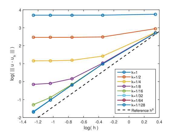
Figure 1: Convergence of model problem end time error in energy norm with respect to the mesh size $h$. For the finite element approximation standard Lagrange $P_{3}$ elements on tetrahedra was used ($p=3$).

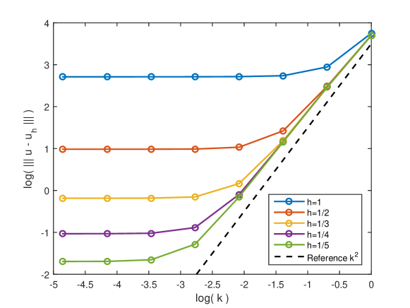
Figure 2: Convergence of model problem end time error in energy norm with respect to the time step $k$. For the finite element approximation standard Lagrange $P_{3}$ elements on tetrahedra was used ($p=3$).

Convergence in ${\bm{L}}^{2}$-norm.

Analogously to the study of the end time error in energy norm we in Figure 3 and Figure 4 provide numerical results for the end time error of the displacements in $L^{2}$ norm. In agreement with Theorem 4.1 these results indicate that the end time $L^{2}$-error estimate for the displacement field should be on the form

$$\|\bm{u}_{0}(T)-\bm{U}_{0}(T)\|_{L^{2}(\Omega)}\lesssim\mathcal{O}(h^{p+1}+k^{2})$$ (5.3)

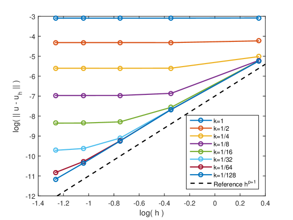
Figure 3: Convergence of model problem end time $L^{2}(\Omega)$-error with respect to the mesh size $h$. For the finite element approximation standard Lagrange $P_{3}$ elements on tetrahedra was used ($p=3$).

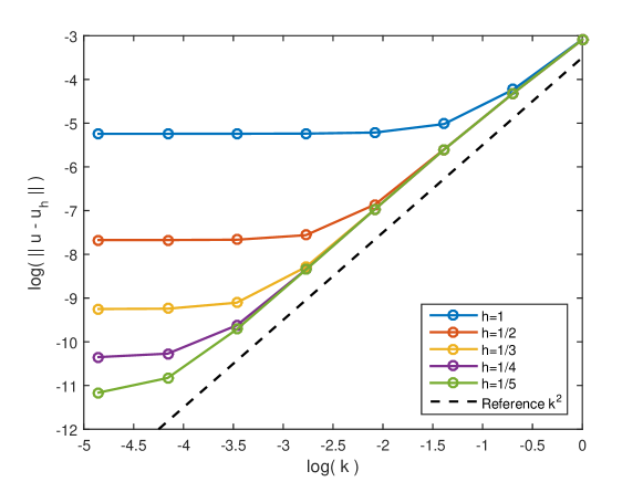
Figure 4: Convergence of model problem end time $L^{2}(\Omega)$-error with respect to the time step $k$. For the finite element approximation standard Lagrange $P_{3}$ elements on tetrahedra was used ($p=3$).

5.2 Energy Conservation

To illustrate Lemma 3.2, the discrete conservation law, we consider the same cube and material as specified in Section 5.1 above. The bottom of the cube ($z=0$) is fixed while $2/5$ of the lid ($z=1$) is prescribed an initial displacement of $\bm{u}_{0}=(0,0,0.20)$ and there are no external forces. The initial deformation in the whole domain is the steady state solution illustrated in Figure 5. Time integration is performed using a time step $k=0.01\mathrm{s}$ and the spatial discretization is done with a mesh size $h=1/5$. After a simulation time of $t=0.1\mathrm{s}$ the prescribed displacement on part of the lid is released and simulation continued until $t=0.5\mathrm{s}$. Recorded energies throughout this simulation is presented in Figure 6. Note that this conservation law is fulfilled independent of the time step.

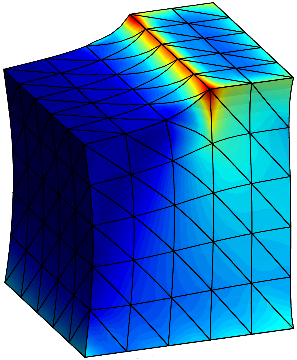
Figure 5: Initial state of deformed unit cube in the conservation law experiment with the color indicating the von Mises stress. Displacements on part of the lid are initially prescribed to $\bm{u}=(0,0,0.20)$ and then released.

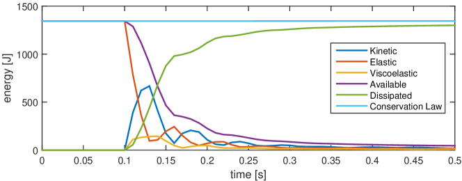
Figure 6: Energies in the discrete conservation law during simulation where an initially deformed cube is released after $t=0.1\mathrm{s}.$

5.3 Numerical Example: A Radial Shaft Seal

Mechanical seals are used in a wide variety of engineering applications when two surfaces need to be joined to prevent leakage, contamination, contain pressure, etc. Due to many preferred properties, such as mechanical damping, viscoelastic elastomers are used when manufacturing seals. It is important that a seal holds tight under expected operational conditions, and therefore accurate description of viscoelastic materials are necessary in the design process.

To demonstrate our viscoelastic model we mimic the following problem: a seal is applied to a vibrating shaft connected to an outer structure, and we wish to investigate the seal holding conditions for a fabricated viscoelastic material under changing shaft vibrations.

As a simple model of a seal we use a pipe geometry with inner radius $0.6\,\mathrm{cm}$, outer radius $1.0\,\mathrm{cm}$ and length $2.0\,\mathrm{cm}$, see Figure 7. We clamp the outer boundary, i.e. impose homogeneous Dirichlet conditions $\bm{u}_{0}=\mathbf{0}$. To simulate the application of the seal on the shaft we apply a slip boundary condition to the inner boundary

$$\bm{u}_{0}\cdot\bm{n} =u_{n}(\bm{x},t)\ ,\qquad(I-\bm{n}\otimes\bm{n})\bm{\sigma}\cdot\bm{n}=\bm{0}\qquad\text{on $\Gamma_{\text{shaft}}$}$$ (5.4)

where the function $u_{n}(\bm{x},t)$ is defined such that the radial displacement yields a cylindrical shape radially expanded by $1\%$ of the inner radius, moving in a circular motion as illustrated in Figure 8. This boundary condition will mimic the shaft’s vibration at different frequencies $\omega$ and the circular motion has an amplitude of $0.1\%$ of the inner radius. As our fabricated material we choose the following parameters: elastic modulus $E=0.5\,\mathrm{MPa}$, Poisson ratio $\nu=0.39$ and viscoelastic parameters found in Table 1. For spatial discretization we use standard Lagrange $P_{2}$ finite elements on tetrahedra. Our model consist of $2880$ elements.

When simulating holding conditions for the seal we measure the contact pressure $P=\bm{n}\cdot\bm{\sigma}\cdot\bm{n}$ and the seal will hold as long as $P\geq 0$. When negative contact pressure arises our simulation is no longer valid as the simulation does not include a contact model, and thus we view any negative contact pressure as an indication of seal failure. In Figure 9 we show the pressure on the inner surface for the frequency $\omega=10\,\mathrm{Hz}$ at four different times during one cycle of vibration.

We investigate the pressure on the inner surface at the end time of three simulations with different frequencies; $1\,\mathrm{Hz}$, $7\,\mathrm{Hz}$ and $15\,\mathrm{Hz}$, as seen in Figure 10. Non-positive pressures are seen in the cases of $7\,\mathrm{Hz}$ and $15\,\mathrm{Hz}$, indicating that the seal might not hold. We then make a sweep over a range of frequencies $\omega=0.01\,\mathrm{Hz}$ to $\omega=1\,\mathrm{kHz}$. During the sweep we measure the pressure at three points near along axial direction; near the end point, at $\nicefrac{{1}}{{4}}$ and $\nicefrac{{1}}{{2}}$ length of the seal. We consider an indication of failure if the pressure in any point goes below zero. We measure during the last cycle for each frequency and plot the minimum and maximum pressures in each point against frequency in Figure 11. From this we see that the minimum pressure goes below zero around $10\,\mathrm{Hz}$ near the end point and up to $1000\,\mathrm{Hz}$ it remains negative. This supports the indication that the seal might be suitable only for frequencies lower than $10\,\mathrm{Hz}$.

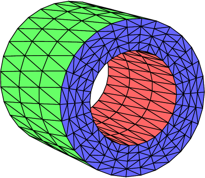
Figure 7: The computational domain of the seal. The clamped surface is green and the red surface is subject to a slip boundary condition and a radial displacement.

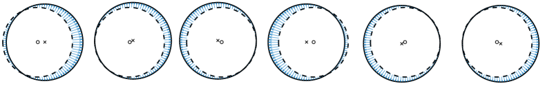
Figure 8: Illustration of the slip boundary condition on the inner surface of the seal. The dashed circle illustrates the surface of the material at rest centered around the small circle. The blue vectors illustrate a prescribed displacement in the surface normal direction such that deformed surface - the solid line - is a circle with larger radius orbiting the center along an elliptical path.

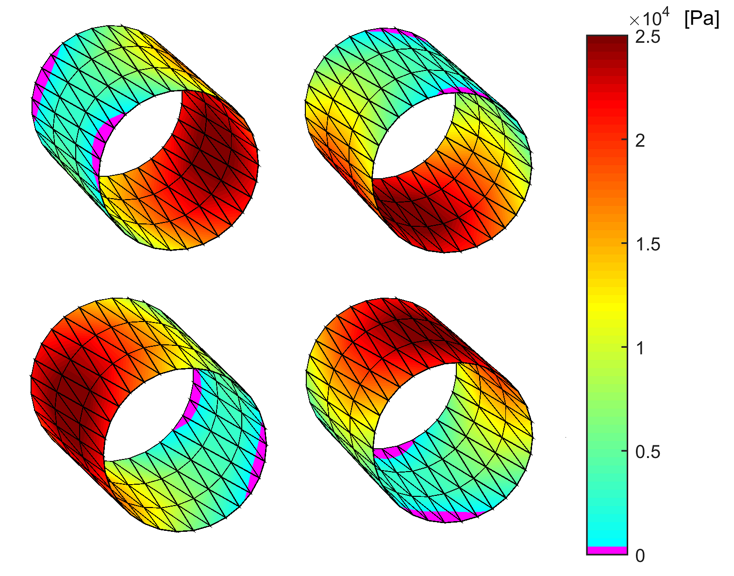
Figure 9: Pressure on inner surface. From top left to bottom right four different states during the last cycle of a run with $10\,\mathrm{Hz}$. Pressure below zero is coloured pink.

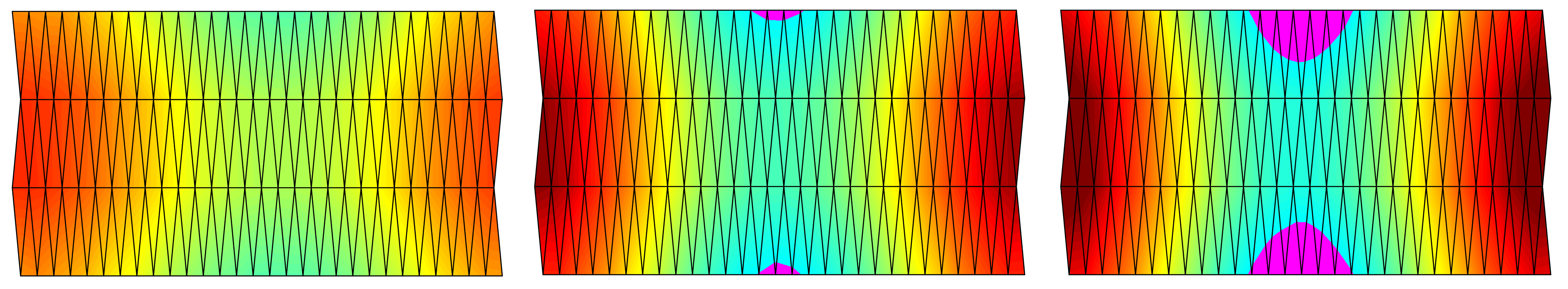
Figure 10: The inner shell of the seal is cut and unwrapped as a plane. The pressure on the inner surface at the last time-step of three simulations. From left to right for the frequencies $1\,\mathrm{Hz}$, $7\,\mathrm{Hz}$, $15\,\mathrm{Hz}$. Pink denotes negative pressure.

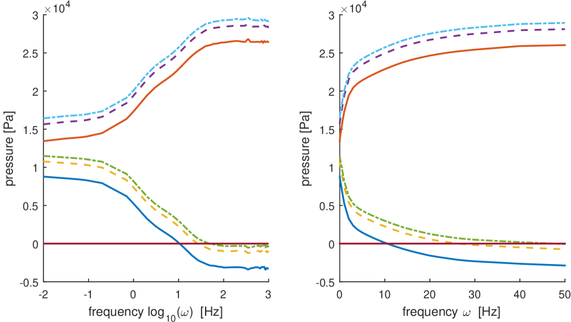
Figure 11: Maximum and minimum contact pressure measured at an endpoint (solid), at a quarter of the seal length (dashed) and mid point (dot–dashed) at different frequencies of the off-center motion of the inner boundary. The left plot shows pressure vs. logarithm frequency spanning $0.01-1000\,\mathrm{Hz}$ and the right plot show pressure vs. frequency zoomed in between $0.01-50\,\mathrm{Hz}$.

Table 1: Viscoelastic parameters for the radial shaft seal problem.

$m$	1	2	3	4	5
$\tau_{m}$ [s]	$1.0\cdot 10^{-2}$	$1.0\cdot 10^{-1}$	$1.0\cdot 10^{0}$	$1.0\cdot 10^{1}$	$1.0\cdot 10^{2}$
$\kappa_{m}$ [Pa]	$3.5\cdot 10^{6}$	$4.0\cdot 10^{6}$	$2.5\cdot 10^{5}$	$2.5\cdot 10^{5}$	$5.0\cdot 10^{5}$

Acknowledgement.

This research was supported in part by the Swedish Research Council Grants Nos.  2017-03911, 2021-04925; and the Swedish Research Programme Essence.

Authors’ addresses:

Martin Björklund   Mathematics and Mathematical Statistics, Umeå University, Sweden
martin.bjorklund@math.umu.se

Karl Larsson,   Mathematics and Mathematical Statistics, Umeå University, Sweden
karl.larsson@umu.se

Mats G. Larson,   Mathematics and Mathematical Statistics, Umeå University, Sweden
mats.larson@umu.se

References

- [1] M. Campo, J. R. Fernández, W. Han, and M. Sofonea. A dynamic viscoelastic contact problem with normal compliance and damage. Finite Elem. Anal. Des., 42(1):1–24, 2005. doi:10.1016/j.finel.2005.04.003.
- [2] K. Eriksson, D. Estep, P. Hansbo, and C. Johnson. Computational Differential Equations. Cambridge University Press, 1996.
- [3] W. Findley, J. Lai, and K. Onaran. Creep and Relaxation of Nonlinear Viscoelastic Materials: With An Introduction To Linear Viscoelasticity. Dover, 1989.
- [4] D. F. Golla and P. Hughes. Dynamics of viscoelastic structures - a time domain, finite element formulation. Journal of Applied Mechanics, 52(4):897–906, 1985.
- [5] Y. Jang and S. Shaw. A priori analysis of a symmetric interior penalty discontinuous Galerkin finite element method for a dynamic linear viscoelasticity model. Comput. Methods Appl. Math., 23(3):647–669, 2023. doi:10.1515/cmam-2022-0201.
- [6] M. Kaliske and H. Rothert. Formulation and implementation of three-dimensional viscoelasticity at small and finite strains. Computational Mechanics, 19(3):228–239, Feb. 1997. doi:10.1007/s004660050171.
- [7] G. A. Lesieutre and E. Bianchini. Time domain modeling of linear viscoelasticity using anelastic displacement fields. Journal of Vibration and Acoustics, 117(4):424–430, 1995.
- [8] G. A. Lesieutre and U. Lee. A finite element for beams having segmented active constrained layers with frequency-dependent viscoelastics. Smart Materials and Structures, 5(5):615–627, 1996.
- [9] D. J. McTavish and P. C. Hughes. Modeling of linear viscoelastic space structures. Journal of Vibration and Acoustics, 115(1):103–113, 1993.
- [10] B. Rivière, S. Shaw, M. F. Wheeler, and J. R. Whiteman. Discontinuous Galerkin finite element methods for linear elasticity and quasistatic linear viscoelasticity. Numer. Math., 95(2):347–376, 2003. doi:10.1007/s002110200394.
- [11] B. Rivière, S. Shaw, and J. R. Whiteman. Discontinuous Galerkin finite element methods for dynamic linear solid viscoelasticity problems. Numer. Methods Partial Differential Equations, 23(5):1149–1166, 2007. doi:10.1002/num.20215.
- [12] M. E. Rognes and R. Winther. Mixed finite element methods for linear viscoelasticity using weak symmetry. Math. Models Methods Appl. Sci., 20(6):955–985, 2010. doi:10.1142/S0218202510004490.
- [13] S. Shaw, M. K. Warby, and J. R. Whiteman. Error estimates with sharp constants for a fading memory Volterra problem in linear solid viscoelasticity. SIAM J. Numer. Anal., 34(3):1237–1254, 1997. doi:10.1137/S003614299528434X.
- [14] S. Shaw, M. K. Warby, J. R. Whiteman, C. Dawson, and M. F. Wheeler. Numerical techniques for the treatment of quasistatic viscoelastic stress problems in linear isotropic solids. Comput. Methods Appl. Mech. Engrg., 118(3-4):211–237, 1994. doi:10.1016/0045-7825(94)90001-9.
- [15] S. Shaw and J. R. Whiteman. Numerical solution of linear quasistatic hereditary viscoelasticity problems. SIAM J. Numer. Anal., 38(1):80–97 (electronic), 2000. doi:10.1137/S0036142998337855.
- [16] H. G. Tillema. Noise reduction of rotating machinery by viscoelastic bearing supports. PhD thesis, SKF Engineering & Research Centre B.V., 2003.
- [17] N. W. Tschoegl. Time Dependence in Material Properties : An Overview. Mechanics of Time-Dependent Materials, 1(1):3–31, 1997.