Visually Guided Object Grasping

Abstract

In this paper we present a visual servoing approach to the problem of object grasping and more generally, to the problem of aligning an end-effector with an object. First we extend the method proposed in [1] to the case of a camera which is not mounted onto the robot being controlled and we stress the importance of the real-time estimation of the image Jacobian. Second, we show how to represent a grasp or more generally, an alignment between two solids in 3-D projective space using an uncalibrated stereo rig. Such a 3-D projective representation is view-invariant in the sense that it can be easily mapped into an image set-point without any knowledge about the camera parameters. Third, we perform an analysis of the performances of the visual servoing algorithm and of the grasping precision that can be expected from this type of approach.

I Introduction

One of the most common tasks in robotics is grasping. Although the importance of grasping has been recognized for many years, there are only a few grasping systems that can operate in complex environments. This is mainly due to the difficulty to execute precise robot hand motions in the presence of various perturbations: the robot’s kinematic is known only partially, unpredictable obstacles may be located in the neighborhood of the object to be grasped, and the location of the object to be grasped with respect to the robot may be either poorly known or not known at all.

Our approach to perform automatic grasping follows the classical approach of splitting the task in off-line and on-line stages. The goal of the off-line stage is to select a grasp – specify a relationship between the gripper and the object – and represent this relationship in some space. The task to be achieved on-line is to control the robot’s motion such that the gripper moves from its initial position to a final position that is consistent with the planned grasp. With our approach both off- and on-line stages use cameras, therefore intrinsic and extrinsic camera calibration will affect the behavior of the grasping process and the accuracy with which the grasping location will eventually be reached. Hence, one of the most important merits of a visually guided grasping technique is to be robust with respect to internal and external camera parameters. Alternatively, one may devise a method which uses uncalibrated cameras.

Consider, for example, the following scenario. The off-line stage – which may well be viewed as a preparation or planning stage – takes place in a laboratory. The on-line stage – task execution – takes place in a hazardous or remote site (nuclear, space, offshore, etc.). The cameras used in the laboratory are not the same as the remote cameras. Moreover, the locations (position and orientation) of the cameras with respect to the object to be grasped and with respect to the robot are not the same in the laboratory and remote site.

In this paper we develop a visual servoing based method that is able of achieving grasping or, more generally, alignment tasks. The main feature of the method described herein is that the accuracy associated with the task to be performed is not affected by discrepancies between the Euclidean setups at task preparation and at task execution stages. By Euclidean setup we mean internal camera calibration and camera-to-world and robot-to-world relationships.

More precisely, the desired object to gripper alignment will be represented in 3-D projective space rather than in 3-D metric space. Such a non-metric representation can be obtained with an uncalibrated pair of cameras, or a stereo rig. During the off-line stage one stereo rig observes both the object and the gripper in their aligned setup and performs a projective reconstruction of both of them. During the on-line stage another stereo rig observes the object and performs its projective reconstruction. Hence, two projective reconstructions of the object are available in two different projective bases, each one of these bases being attached to each one of the two stereo rigs. Therefore it is possible to compute a 3-D projective transformation between the off-line and on-line setups, transfer the gripper from one setup to another, and predict the location of the gripper in the images associated with the second stereo rig. Once this off-line to on-line transfer of gripper points from one image pair to another image pair has been performed, the problem of moving the gripper from an initial position to the desired grasp position becomes a classical image-based robot servoing problem:

1. estimate the velocity screw associated with the gripper frame;

2. move the robot until the image points associated with the observed gripper are properly aligned with their predicted locations.

The visual grasping scheme that we just described suggests that:

1. two cameras are involved in the visually guided control loop;

2. these cameras must be calibrated [2].

In fact, once the gripper points have been properly transferred, the visual servoing process can proceed with only one of the two cameras and hence, only one among these two cameras must be internally calibrated. Recently it has been shown by one of us that internal camera calibration weakly affects the convergence of image-based robot control when only one camera is being used [3].

II Background, contribution, and paper organization

The theory of image-based servoing has been developed, in parallel, by a number of researchers [1], [4], [5], [6], [7], [8], [9], [10]. Central to the image-based approach is the necessity to compute the image Jacobian. This is equivalent to computing the differential relationship between a scene frame and the camera frame (either the scene or the camera frame is attached to the robot). Jacobian estimation requires knowledge about the camera intrinsic and extrinsic parameters. The latter parameters amount to the rigid mapping between the scene frame and the camera frame. Many implementations get around this problem by simply allocating constant values to the image Jacobian.

The debate whether the sensor should be mounted onto the robot (eye-in-hand) or should be mounted onto a fixture (independent-eye) is important because each one of these two setups has limitations and advantages. With a hand-eye approach, the setup (camera parameters and hand-eye relationship) at planning must be identical with the setup at runtime. The independent eye approach offers more flexibility at the price of the use of several cameras rather than a single camera.

This paper has the following contributions. In section III we extend the hand-eye servoing method proposed in [1] to the independent-eye setup. Within the context of the new mathematical expression that we derive for the image Jacobian, we make clear which parameters vary with time and which parameters remain constant. Indeed, in a recent review paper [2] this analysis was not available. Moreover we stress the importance of on-line pose computation.

In section IV we show how to represent an alignment between two objects in 3-D projective space. The alignment condition thus derived is projective invariant in the sense that it can be used in conjunction with two uncalibrated camera pairs (one at planning and one at runtime) to compute a goal position for visual servoing.

In sections V and VI we describe an in depth comparison of image-based servoing with a fixed (approximated) Jacobian and with a variable (exact) Jacobian. Next we describe the implementation of a visually-guided grasping system which integrates the results of sections III, IV, together with a pose computation method. Finally, section VII gives some directions for future work.

III Image-based servoing

In this section we consider a camera that observes a moving robot gripper. First we determine the image Jacobian associated with such a configuration. Second we define a visual servoing process that allows the camera to control the robot motion such that the gripper reaches a previously determined image set position – one way to compute such an image set position using an uncalibrated stereo rig will be described in section IV.

III-A Image Jacobian

Let us define two useful Euclidean frames as follows, Figure 1:

1. $F_{g}^{0}$ is the gripper reference frame associated with the gripper in its initial position prior to visual servoing and

2. $F_{c}^{0}$ is the camera reference frame; since the camera will remain fixed while the gripper will move, the frame attached to the camera is a fixed reference frame.

Let $\mbox{\bf D}^{gc}$ be the 4$\times$4 homogeneous matrix mapping $F_{g}^{0}$ onto $F_{c}^{0}$. Next we consider the gripper while it moves and we define two moving frames rigidly attached to the gripper:

1. $F_{g}$ which is a moving gripper frame related to $F_{g}^{0}$ by the continuous displacement $\mbox{\boldmath$D$}^{g}(t):F_{g}^{0}\rightarrow F_{g}$ and

2. $F_{c}$ which as a moving frame as well rigidly attached to the gripper related to $F_{c}^{0}$ by the continous displacement $\mbox{\boldmath$D$}^{c}(t):F_{c}^{0}\rightarrow F_{c}$.

Clearly the homogeneous matrix mapping $F_{g}$ onto $F_{c}$ is the same as the matrix mapping $F_{g}^{0}$ onto $F_{c}^{0}$ and is equal to:

$$\mbox{\bf D}^{gc}=\left(\begin{array}[]{cc}\mbox{\bf R}^{gc}&\mbox{\boldmath$t$}^{gc}\\ \mbox{\boldmath$0$}^{\top}&1\end{array}\right)$$ (1)

At each time $t$ the two displacements $\mbox{\boldmath$D$}^{g}(t)$ and $\mbox{\boldmath$D$}^{c}(t)$ are conjugated:

$$\mbox{\boldmath$D$}^{c}(t)=(\mbox{\bf D}^{gc})^{-1}\;\mbox{\boldmath$D$}^{g}(t)\;\mbox{\bf D}^{gc}$$

Consequently the motion of the gripper can be expressed either by the moving frame $F_{g}$ with respect to $F_{g}^{0}$ or by the moving frame $F_{c}$ with respect to $F_{c}^{0}$:

$$\mbox{\boldmath$T$}_{g}=\{\mbox{\boldmath$V$}(O_{g}),\Omega_{g}\}$$

is the velocity screw of $F_{g}$ with respect to $F_{g}^{0}$ and

$$\mbox{\boldmath$T$}_{c}=\{\mbox{\boldmath$V$}(O_{c}),\Omega_{c}\}$$

is the velocity screw of $F_{c}$ with respect to $F_{c}^{0}$. These two screws are related by the formula:

$$\mbox{\boldmath$T$}_{c}=\Theta^{gc}\mbox{\boldmath$T$}_{g}$$ (2)

with:

$$\Theta^{gc}=\left(\begin{array}[]{cc}\mbox{\bf R}^{gc}&\mbox{\bf R}^{gc}S(\mbox{\boldmath$t$}^{gc})\\ \mbox{\boldmath$0$}&\mbox{\bf R}^{gc}\end{array}\right)$$ (3)

where $S(\mbox{\boldmath$a$})$ is the skew-symmetric matrix associated with a 3-vector $a$. It is important to notice that the rotation $\mbox{\bf R}^{gc}$ and translation $\mbox{\boldmath$t$}^{gc}$ describe the initial pose of the gripper with respect to the camera and hence they remain constant during visual servoing.

Now, let $B_{j}$ be a 3-D point onto the gripper and let $\mbox{\boldmath$B$}_{j}^{c}=(x_{j},y_{j},z_{j})^{\top}$ be its Euclidean coordinates in the camera-centered frame $F_{c}^{0}$, e.g., figure 1. The projection of this point onto the image has as coordinates:

$$u_{j} = \alpha_{u}\frac{x_{j}}{z_{j}}+u_{0}$$ (4)

$$v_{j} = \alpha_{v}\frac{y_{j}}{z_{j}}+v_{0}$$ (5)

where $\alpha_{u}$, $\alpha_{v}$, $u_{0}$, and $v_{0}$ are the well known intrinsic camera parameters associated with a pin-hole model and $(u,v)$ are the image coordinates of a pixel. By computing the time derivatives of $u_{j}$ and $v_{j}$ in equations (4) and (5), knowing that $\stackrel{{\scriptstyle\bullet}}{{\mbox{\boldmath$B$}_{j}^{c}}}=\mbox{\boldmath$V$}(O_{c})+\Omega_{c}\times\mbox{\boldmath$B$}_{j}^{c}$, and by combining with eq. (3), it is straightforward to obtain:

$$\left(\begin{array}[]{c}\stackrel{{\scriptstyle\bullet}}{{u}}_{j}\\ \stackrel{{\scriptstyle\bullet}}{{v}}_{j}\end{array}\right)=\mbox{\bf J}_{j}\mbox{\boldmath$T$}_{g}$$ (6)

with $\mbox{\bf J}_{j}=\mbox{\bf L}_{j}\Theta^{gc}$ and $\mbox{\bf L}_{j}$ equal to:

$$\left(\begin{array}[]{cc}\alpha_{u}&0\\ 0&\alpha_{v}\end{array}\right)\left(\begin{array}[]{cccccc}\frac{1}{z_{j}}&0&\frac{-x_{j}}{z_{j}^{2}}&\frac{-x_{j}y_{j}}{z_{j}^{2}}&1+\frac{x_{j}^{2}}{z_{j}^{2}}&\frac{-y_{j}}{z_{j}}\\ 0&\frac{1}{z_{j}}&\frac{-y_{j}}{z_{j}^{2}}&-1-\frac{y_{j}^{2}}{z_{j}^{2}}&\frac{x_{j}y_{j}}{z_{j}^{2}}&\frac{x_{j}}{z_{j}}\end{array}\right)$$

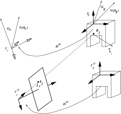
Figure 1: This figure shows the relationships between the various frames associated with the gripper and with the camera.

III-B Control law

As already mentioned, we consider $n$ 3-D points ($B_{j}$) onto the robot gripper together with their projections onto the image ($\mbox{\boldmath$b$}_{j}=(s\,u_{j},\;s\,v_{j},\;s)$). Let $s$ be the image vector formed with the Euclidean coordinates of all the points $\mbox{\boldmath$b$}_{j}$. For $n$ points, the vector $s$ has 2$\times n$ components:

$$\mbox{\boldmath$s$}=\left(u_{1}\;v_{1}\ldots u_{j}\;v_{j}\ldots u_{n}\;v_{n}\right)^{\top}$$

We denote by $\mbox{\boldmath$s$}^{\star}$ the image set-point – the final (goal) position. This goal position may correspond, for example, to an alignment condition for grasping (see section IV) or to any other goal position that one wants to reach.

Therefore, the task consists in moving the robot such that the Euclidean norm of the error vector $\mbox{\boldmath$s$}-\mbox{\boldmath$s$}^{\star}$ decreases. Hence, one may constrain the image velocity of each point being considered to exponentially reach its goal position with time. This desired behavior writes as $\stackrel{{\scriptstyle\bullet}}{{\mbox{\boldmath$s$}}}=g\left(\mbox{\boldmath$s$}^{\star}-\mbox{\boldmath$s$}\right)$ where $g$ is a positive scalar that controls the convergence rate of the visual servoing.

It is now possible to combine the above formula with eq. (6) and we obtain:

$$\mbox{\bf J}\mbox{\boldmath$T$}_{g}=g\left(\mbox{\boldmath$s$}^{\star}-\mbox{\boldmath$s$}\right)$$ (7)

With $\mbox{\bf J}^{\top}=\left(\mbox{\bf J}_{1}^{\top}\ldots\mbox{\bf J}_{n}^{\top}\right)$. Let us now assume that the rank of the $n\times$6 matrix J is 6 (i.e $n\geq 3$, and the gripper points $B_{j}$ are not collinear). The control velocity screw may then be computed as:

$$\mbox{\boldmath$T$}_{g}=g\left(\hat{\mbox{\bf J}}^{\top}\mbox{\bf W}\hat{\mbox{\bf J}}\right)^{-1}\hat{\mbox{\bf J}}^{\top}W\left(\mbox{\boldmath$s$}^{\star}-\mbox{\boldmath$s$}\right)=g\hat{\mbox{\bf J}}^{\dagger}\left(\mbox{\boldmath$s$}^{\star}-\mbox{\boldmath$s$}\right)$$ (8)

where W is a symmetric positive matrix of rank 6 allowing, for example, to select some preferred points in the image among the $n$ points that are available, and $\hat{\mbox{\bf J}}$ is the model of J which is used in the control expression.

To compute this model $\hat{\mbox{\bf J}}$, it is therefore necessary to estimate the constant matrix $\Theta^{gc}$ and the time-varying values of $x_{j}$, $y_{j}$, and $z_{j}$ in $F_{c}$.

Let $\mbox{\boldmath$B$}_{j}^{g}$ be the coordinates of a gripper point in the gripper frame $F_{g}$. These coordinates can be easily estimated off-line using a hand-tool calibration technique and which is described in [11]. In order to estimate the initial pose of the gripper with respect to the camera, i.e., $\mbox{\bf D}^{gc}$, one has to apply a pose computation method to a set of 2-D to 3-D point matches $\mbox{\boldmath$b$}_{j}\leftrightarrow\mbox{\boldmath$B$}_{j}^{g}$ when the gripper is in its initial position. Moreover, $x_{j}$, $y_{j}$, $z_{j}$ – the camera coordinates of $B_{j}$ can also be evaluated through a pose computation method, the pose method being applied at each time to the matches $\mbox{\boldmath$b$}_{j}\leftrightarrow\mbox{\boldmath$B$}_{j}^{g}$.

Pose computation is a classical problem in computer vision and photogrammetry and many closed-form and/or numerical solutions have been proposed in the past. Nevertheless, these solutions to the object pose computation problem were not entirely satisfactory. This is the main reason for which the current solution used in visual servoing consists in considering that the pose parameters do not vary too much over time and hence $\hat{\mbox{\bf J}}$ is often obtained by giving to the entries of J constant values, for example those corresponding to the goal position [1]. Even if the stability of the closed loop system can be preserved as long as $\mbox{\bf J}\hat{\mbox{\bf J}}^{\dagger}$ is a positive matrix, the convergence can nevertheless be strongly affected. In [12] we present a new object pose computation method that is fast and reliable enough to be incorporated in the real-time loop of the visual servoing algorithm and it will be shown in the following that its performances will be significantly improved compared to the classical approach.

IV Projective invariant object/gripper alignment

The visual servoing method described in the previous section requires knowledge of the set-point $\mbox{\boldmath$s$}^{\star}$ which is a set of image points. $\mbox{\boldmath$s$}^{\star}$ is a function of the camera/gripper relationship (extrinsic parameters) and of the camera internal model (intrinsic parameters). Whenever the location of the object to be grasped varies with respect to the camera, the set-point $\mbox{\boldmath$s$}^{\star}$ varies as well. In this section we show how to compute the set-point $\mbox{\boldmath$s$}^{\star}$ such that it is “view-invariant”, i.e., it is independent of both intrinsic and extrinsic camera parameters. This will allow more flexibility because the setups at learning and runtime stages can be different.

In Euclidean space, the relationship between two objects is usually represented by some rigid transformation. Alternatively, the object-gripper alignment, or any other object-to-object relationship, can be represented in terms of relationships between objects points. The choice of these points depends upon the visual sensor being used and hence upon the visual process allowing to extract image points, i.e., feature extraction. They are not necessarily contact points between the object and the gripper. Therefore they may not be present in the CAD descriptions of both the object and the gripper. The idea of our approach is to represent such object-gripper relationships projectively: 3-D object and gripper points are described into an object-centered projective basis.

Figure 2: The object projective basis is rigidly attached to the gripper Euclidean frame. Whenever the object moves, these two frames remain virtually attached to it. The projective mapping is conjugated to the Euclidean mapping.

More precisely, consider an object to be grasped and a gripper aligned with this object. Let $A_{i},\;i=1\ldots m$ be a set of 3-D object points and $B_{j},\;j=1\ldots n$ be a set of 3-D gripper points. Among the object points consider five of them in general position, say $A_{1}$ to $A_{5}$ (these five points form a basis of the 3-D projective space) and let $\mbox{\boldmath$A$}^{o}_{i}$, $\mbox{\boldmath$B$}^{o}_{j}$ be the projective coordinates of the object and gripper points in this basis. Moreover, consider an Euclidean frame attached to the gripper, $F_{g}$. Three points are sufficient to uniquely define such an Euclidean frame. Notice that an Euclidean frame is just a special case of a projective basis where one point is the origin of the frame, three points on the plane at infinity correspond to the directions of the three axes, and the fifth point defines the unit vector [13].

Therefore, the Euclidean space can be viewed as a subspace of the projective space. There exists a projective transformation mapping Euclidean coordinates onto projective coordinates. Such a transformation is conveniently described by a 4$\times$4 invertible homogeneous matrix and let $\mbox{\bf H}^{go}$ be the matrix mapping Euclidean coordinates onto projective coordinates from the gripper frame onto the object basis described above. If we denote by $\mbox{\boldmath$A$}^{e}_{i}$, $\mbox{\boldmath$B$}^{e}_{j}$ the Euclidean coordinates of the points just mentioned we have:

$$\mbox{\boldmath$A$}^{o}_{i}\simeq\mbox{\bf H}^{go}\mbox{\boldmath$A$}^{e}_{i}$$

$$\mbox{\boldmath$B$}^{o}_{j}\simeq\mbox{\bf H}^{go}\mbox{\boldmath$B$}^{e}_{j}$$

where “$\simeq$” denotes the projective equality.

Next we suppose that the object alone lies in a different position and orientation. Therefore, the object moved and since its motion is a rigid one it can be described in the Euclidean frame mentioned above which remained virtually linked to the object. Let D be the rigid motion associated with the object and with this particular frame. D is a 4$\times$4 homogeneous mapping of the form given by eq. (1). The equivalent projective displacement is (see Figure 2):

$$\mbox{\bf H}\simeq\mbox{\bf H}^{go}\mbox{\bf D}\left(\mbox{\bf H}^{go}\right)^{-1}$$

H maps the “old” projective coordinates into the “new” ones and D maps the old Euclidean coordinates into the new ones but the relationship between the Euclidean and projective representations of the gripper-to-object alignment, $\mbox{\bf H}^{go}$ remains invariant. In practice this representation is encapsulated by the projective coordinates of gripper points in an object centered projective basis: $\mbox{\boldmath$B$}_{1}^{o},\;\ldots\mbox{\boldmath$B$}_{n}^{o}$ in the projective basis $\mbox{\boldmath$A$}_{1}^{o},\;\ldots\mbox{\boldmath$A$}_{5}^{o}$.

IV-A Projective reconstruction with a camera pair

We consider a pair of uncalibrated cameras which observe the gripper aligned with the object, Figure 3. It is known that from point-to-point matches between the two images it is possible to compute the epipolar geometry associated with the two cameras [14]. Moreover, from the epipolar geometry two 3$\times$4 projection matrices mapping the 3-D projective space onto the two images can be computed [15]. We denote by $\mbox{\bf P}^{x}$ and $\mbox{\bf P}^{\prime x}$ the two projection matrices. Let $\mbox{\boldmath$m$}^{x}$ and $\mbox{\boldmath$m$}^{\prime x}$ be the projections of a 3-D point $M$ onto the left and right images associated with the two cameras. The equations:

$$\mbox{\boldmath$m$}^{x}\simeq\mbox{\bf P}^{x}\mbox{\boldmath$M$}^{x},\;\;\mbox{\boldmath$m$}^{\prime x}\simeq\mbox{\bf P}^{\prime x}\mbox{\boldmath$M$}^{x}$$ (9)

allow to compute the 3-D projective coordinates $\mbox{\boldmath$M$}^{x}$ of the 3-D point $M$ in a projective basis $x$ attached to the camera pair. Since the geometry of the camera pair (intrinsic and extrinsic parameters) may change over time, the camera pair is not a rigid object. However it is possible to compute a projective transformation mapping the sensor centered projective reconstruction $x$ into the object centered projective reconstruction $o$ just described. For the sensor and object projective coordinates of a point $A_{i}$ we have:

$$\mbox{\boldmath$A$}^{o}_{i}\simeq\mbox{\bf H}^{xo}\mbox{\boldmath$A$}^{x}_{i}$$ (10)

where $\mbox{\boldmath$A$}^{x}_{i}$ is obtained by applying eq. (9) to an object point being observed with the camera pair, and $\mbox{\bf H}^{xo}$ is a 4$\times$4 projective transformation.

IV-B Stereo point transfer

At runtime, another stereo pair observes the object to be grasped. However, the gripper is at some distance from the object and the task is to move the gripper from its initial position to a virtual position. The latter gripper position corresponds to the gripper-to-object alignment defined during the off-line stage.

Let $\mbox{\bf P}^{y}$ and $\mbox{\bf P}^{\prime y}$ be the matrices associated with the runtime camera pair $y$ and therefore we have:

$$\mbox{\boldmath$m$}^{y}\simeq\mbox{\bf P}^{y}\mbox{\boldmath$M$}^{y},\;\;\mbox{\boldmath$m$}^{\prime y}\simeq\mbox{\bf P}^{\prime y}\mbox{\boldmath$M$}^{y}$$ (11)

Again, the sensor centered 3-D projective coordinates of an object point can be mapped in a object centered description:

$$\mbox{\boldmath$A$}^{o}_{i}\simeq\mbox{\bf H}^{yo}\mbox{\boldmath$A$}^{y}_{i}$$ (12)

By combining eqs. (10) and (12) we obtain a relationship between the projective coordinates of an object point expressed in the two projective bases $x$ and $y$:

$$\mbox{\boldmath$A$}^{y}_{i}\simeq\left(\mbox{\bf H}^{yo}\right)^{-1}\mbox{\bf H}^{xo}\mbox{\boldmath$A$}^{x}_{i}\simeq\mbox{\bf H}^{xy}\mbox{\boldmath$A$}^{x}_{i}$$ (13)

Figure 3: The projective basis in which the camera pair reconstructs scene points is a sensor centered basis. Alternatively, one can select five points onto the object to be grasped and built an object centered representation of the gripper-to-object alignment.

Eq. (13) allows to compute a 4$\times$4 homogeneous matrix $\mbox{\bf H}^{xy}$ from point matches between two setups, $x$ and $y$, $(\mbox{\boldmath$a$}^{x},\mbox{\boldmath$a$}^{\prime x})\leftrightarrow(\mbox{\boldmath$a$}^{y},\mbox{\boldmath$a$}^{\prime y})$. With five point matches one obtains an exact solution. However, if a larger number of point matches are available, a least-square solution can be computed [16]. To summarize, the following procedure transfers gripper points from the learning setup to the runtime setup:

1. For each gripper point $B_{j},\;j=1\ldots n$:

2. Reconstruct the projective coordinates of a gripper point from its images associated with the setup $x$:

   $$\mbox{\boldmath$b$}^{x}_{j}\simeq\mbox{\bf P}^{x}\mbox{\boldmath$B$}^{x}_{j},\;\;\mbox{\boldmath$b$}^{\prime x}_{j}\simeq\mbox{\bf P}^{\prime x}\mbox{\boldmath$B$}^{x}_{j}$$

3. Map these point coordinates from one projective basis to the other projective basis:

   $$\mbox{\boldmath$B$}^{y}_{j}\simeq\mbox{\bf H}^{xy}\mbox{\boldmath$B$}^{x}_{j}$$

4. Project the gripper point onto the images associated with the runtime setup:

   $$\mbox{\boldmath$b$}^{y}_{j}\simeq\mbox{\bf P}^{y}\mbox{\boldmath$B$}^{y}_{j},\;\;\mbox{\boldmath$b$}^{\prime y}_{j}\simeq\mbox{\bf P}^{\prime y}\mbox{\boldmath$B$}^{y}_{j}$$

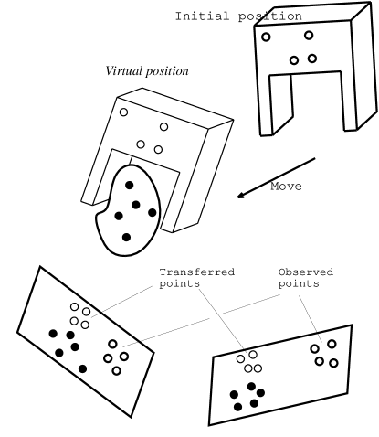
Figure 4: This figure shows the runtime setup where the gripper is visually servoed from an initial to a goal position. The goal position is defined by the image transferred point, or implicitly by a 3-D virtual position of the gripper.

IV-C Computing the set-point $\mbox{\boldmath$s$}^{\star}$

The set-point $\mbox{\boldmath$s$}^{\star}$ is simply derived by transforming the 2-D homogeneous coordinates of an image point into its image coordinates:

$$\mbox{\boldmath$s$}^{\star}=\left(\begin{array}[]{c}\widetilde{\mbox{\boldmath$b$}_{1}^{x}}\\ \vdots\\ \widetilde{\mbox{\boldmath$b$}_{n}^{x}}\end{array}\right)\mbox{ with }\mbox{\boldmath$b$}_{j}^{x}=\lambda\left(\begin{array}[]{c}\widetilde{\mbox{\boldmath$b$}_{1}^{x}}\\ 1\end{array}\right)$$

In theory the visual servoing algorithm described in section III needs a single camera. Therefore a minimal camera configuration may consist in one camera pair at planning and a single camera at runtime: indeed, it is possible to combine the runtime camera with any one of the two other cameras to perform the transfer and compute the set-point. Alternatively, one can run two simultaneous visual servoing processes and with two cameras eq. (8) becomes:

$$\mbox{\boldmath$T$}_{g}=g\left(\begin{array}[]{cc}\hat{\mbox{\bf J}}^{\dagger}&\hat{\mbox{\bf J}}^{\prime{\dagger}}\end{array}\right)\left(\begin{array}[]{c}\mbox{\boldmath$s$}^{\star}-\mbox{\boldmath$s$}\\ \mbox{\boldmath$s$}^{\prime\star}-\mbox{\boldmath$s$}^{\prime}\end{array}\right)$$

V Performance analysis

In this section we analyze the behavior of the visual servoing algorithm described in section III. This algorithm is given an image set-point $\mbox{\boldmath$s$}^{\star}$ and a current image position $s$ and attempts to align $s$ with $\mbox{\boldmath$s$}^{\star}$. This alignment is done according to eq. (8): the robot moves until the norm of the image error vector $\mbox{\boldmath$s$}^{\star}-\mbox{\boldmath$s$}$ vanishes. Therefore, a good estimation, $\hat{\mbox{\bf J}}^{\dagger}$, of the pseudo-inverse of J, is key. As already mentioned, the classical approach used as an estimation of $\hat{\mbox{\bf J}}$ is the measured value of J at the equilibrium configuration — the robot lies in the desired goal position. Hence, with this choice, $\hat{\mbox{\bf J}}^{\dagger}$ is kept constant during all the servoing process.

The pose algorithm introduced in [12] allows us to compute on-line a current estimate of $\mbox{\bf J}^{\dagger}$ in approximatively $2\;10^{-3}$ seconds. This computation time is compatible with real-time feature tracking and servoing. It is therefore possible to run experiments in order to analyze the behavior of visual servoing with an updated Jacobian.

Unlike the computation of the set-point $\mbox{\boldmath$s$}^{\star}$, both methods (updated and constant Jacobians) require explicit values for the camera intrinsic parameters. However, in [3] is shown that the convergence of visual servoing is very little affected by these parameters. In practice we used the horizontal and vertical focal lengths provided by the camera manufacturer and we set the position of the optical axis at the image center: $\alpha_{u}=1500,\;\;\alpha_{v}=1000,\;\;u_{0}=v_{0}=256$

In order to compare the behavior of the variable Jacobian servoing with the constant Jacobian servoing we performed the following experiments. In the first experiment the distance between the initial and final robot position is “small” (15⁰ in orientation and 35cm in depth). In the second experiment this distance is large (30⁰ in orientation and 70cm in depth). The curves plotted on Figure 5 represent the norm of the image error ($\|\mbox{\boldmath$s$}^{\star}-\mbox{\boldmath$s$}\|$) between the current gripper position and the final gripper position as a function of time.

One may notice that, in both experiments described above, the variable-Jacobian servoing algorithm has an exponential error decrease associated with it, which is not the case for the constant-Jacobian servoing and for large depth discrepancies between the initial and goal positions.

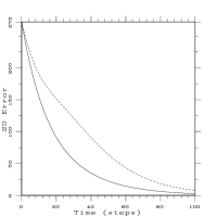
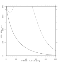
Figure 5: These plots show the behavior of the servoing algorithm when the distance between the initial and final gripper position is “small” (left) and when this distance is “large” (right). The full curves correspond to exact Jacobian servoing while the dashed curves correspond to a constant Jacobian servoing.

The visual servoing algorithm runs at 10Hz on a Sun/Sparc10 workstation. Table I summarizes the CPU times associated with each stage of the algorithm. Notice that 70% of the computing power is devoted to data transfer (image acquisition, image transfer, computer-robot communications) and only 2% is devoted to the on-line computation of the image Jacobian.

TABLE I: One cycle of the real-time control loop.

Image acquisition	40ms
Image transfer	20ms
Image processing	30ms
Jacobian computation	2ms
Velocity screw computation	1ms
Computer-robot communication	10ms
Total	103ms

VI Grasping experiments

As already described, grasping includes a planning stage, a transfer stage, and an execution stage. The execution stage performs a real-time visually controlled loop:

• At planning time an uncalibrated stereo rig computes a 3-D projective representation of grasping. This is illustrated on Figure 6.

• At preparation time a single camera observes both the object to be grasped and the gripper in some initial position. The locations of both the object and the gripper are arbitrary, provided that they are in the field of view of the camera. The goal of this preparation stage is to transfer gripper points in order to compute the image set-point $\mbox{\boldmath$s$}^{\star}$ – Figure 7–left.

• The robot motion can now be controlled using visual feedback. The velocity screw associated with the gripper frame is iteratively updated using eq. (8) until the norm of the image error vector $\|\mbox{\boldmath$s$}^{\star}-\mbox{\boldmath$s$}\|$ vanishes. Figure 7–right shows the final grasping location reached by the gripper.

Since only one camera is used at runtime, the image point transfer technique combines this camera with the camera pair used off-line to form two stereo pairs.

Figure 6: The gripper and the object to be grasped as viewed by a stereo rig. A large set of point correspondences (not shown) allows us to compute the epipolar geometry. Object points together with gripper points are represented in a 3-D projective space.

Figure 7: An example of applying the visually guided grasping method. The set-point (left) is the projection of a view-invariant alignment representation. The grasp (right) is reached when the image of the gripper is aligned with the set-point.

One important feature of any grasping method is the precision with which the gripper and the object are eventually aligned. In all our experiments the distance from the camera to the object to be grasped is of approximatively 1 meter. The camera lens has a focal length of 12.5 mm ($\alpha_{u}\approx 1000$) which allows for a wide field of view. Since the method’s main idea is to align image points, the final grasping overall precision depends on the quality of the set-point $\mbox{\boldmath$s$}^{\star}$. When the gripper is properly aligned with the object to be grasped, a gripper point with camera coordinates $(x,y,z)$ matches an image point with coordinates $(u,v)$ and this image point belongs to the set-point $\mbox{\boldmath$s$}^{\star}$. We establish the relationship between the 3-D error and the 2-D error.

By differentiation of eq. (4) we obtain the following relationship:

$$du=\alpha_{u}\left(\frac{dx}{z}-\frac{x\;dz}{z^{2}}\right)$$

The 3-D precision that we want to achieve is 0.5 mm. Therefore we have $dx=dz=5\;10^{-4}$m, and let $x=0.1$m, $z=1$m, $\alpha_{u}=1000$. We obtain: $du\approx dv\approx 0.5\mbox{\rm pixels}$ This means that the transfer method outlined above must compute the set-point with an accuracy of $0.5$ pixels. Such an accuracy may be obtained, provided that (i) the image locations of object points have an equivalent accuracy and (ii) there are 15 to 20 object points available with the image pairs [16]. The first condition can be easily satisfied with standard correlation-based point-feature extraction methods. The second condition is more difficult to satisfy because it is context dependent.

VII Discussion

We described a method for aligning a robot end-effector with an object. An example of such an alignment is grasping. The method consists of using an uncalibrated stereo rig in order to represent the alignment in 3-D projective space and of servoing the robot using visual feedback from either one or two cameras. As already mentioned, the set-point – the set of image points with which the gripper points must eventually be aligned – can be computed without any camera calibration. The final accuracy of the gripper-to-object alignment depends on the accuracy with which the set-point has been estimated. Nevertheless, the computation of the image Jacobian requires the camera intrinsic parameters to be known. The accuracy of these parameters does not affect neither the final precision of the alignment nor the convergence of the servoing algorithm; they merely affect the trajectory of the gripper between its initial and goal locations.

One interesting feature of the method is that no Euclidean knowledge about the object to be grasped is required. In order to relate the velocity screw of the gripper with the image error vector the method requires Euclidean knowledge about the robot gripper, namely the Euclidean coordinates of the gripper markings must be known in gripper frame. This is an intrinsic property of the gripper that can be easily determined using standard hand-eye or hand-tool calibration methods [17], [11].

The use of visual feedback for object grasping and for alignment in general is a promising research topic because it is a tolerant to various disturbances and because it does not require such prior knowledge as robot-to-world calibration and/or CAD models for the objects to be manipulated. The method described in this paper permits a deeper understanding of the interaction between uncalibrated vision and robot control which has important implications in robotics.

References

- [1] B. Espiau, F. Chaumette, and P. Rives, “A new approach to visual servoing in robotics,” IEEE Transactions on Robotics and Automation, vol. 8, no. 3, pp. 313–326, June 1992.
- [2] S. Hutchinson, G. D. Hager, and P. I. Corke, “A tutorial on visual servo control,” IEEE Transactions on Robotics and Automation, vol. 12, no. 5, pp. 651–670, October 1996.
- [3] B. Espiau, “Effect of camera calibration errors on visual servoing in robotics,” in Proceedings of the Third International Symposium on Experimental Robotics, Kyoto, Japan, October 1993, pp. 187–193.
- [4] K. Hashimoto, T. Kimoto, T. Ebine, and H. Kimura, “Manipulator control with image-based visual servo,” in Proceedings of the 1991 IEEE International Conference on Robotics and Automation, Sacramento, California, April 1991, vol. 3, pp. 2267–2272.
- [5] N. Maru, H. Kase, S. Yamada, A. Nishikawa, and F. Miyazaki, “Manipulator control by visual servoing with the stereo vision,” in Proceedings of the 1993 IEEE/RSJ International Conference on Intelligent Robots and Systems, Yokohama, Japan, July 1993, vol. 3, pp. 1866–1870.
- [6] G. D. Hager, G. Grunwald, and G. Hirzinger, “Feature-based visual servoing and its application to telerobotics,” in Proceedings of the IEEE/RSJ/GI International Conference on Intelligent Robots and Systems, September 1994, vol. 1, pp. 164–171.
- [7] J. T. Feddema, C. S. G. Lee, and O. R. Mitchell, “Feature-based visual servoing of robotic systems,” in Visual Servoing, K. Hashimoto, Ed., pp. 105–138. World Scientific, 1993.
- [8] P. I. Corke, “Visual control of robot manipulators – a review,” in Visual Servoing, K. Hashimoto, Ed., pp. 1–32. World Scientific, 1993.
- [9] P. I. Corke, “Video-rate robot visual servoing,” in Visual Servoing, K. Hashimoto, Ed., pp. 257–283. World Scientific, 1993.
- [10] R. Sharma and S. Hutchinson, “On the observability of robot motion under active camera control,” in Proceedings of the 1994 IEEE International Conference on Robotics and Automation, San Diego, California, May 1994, vol. 1, pp. 162–167.
- [11] F. Dornaika and R. Horaud, “Simultaneous robot-world and hand-eye calibration,” IEEE Transactions on Robotics and Automation, 1998, To appear.
- [12] R. Horaud, F. Dornaika, B. Lamiroy, and S. Christy, “Object pose: The link between weak perspective, paraperspective, and full perspective,” International Journal of Computer Vision, vol. 22, no. 2, pp. 173–189, March 1997.
- [13] J.G. Semple and G.T. Kneebone, Algebraic Projective Geometry, Clarendon Press, Oxford, Great Britain, 1979.
- [14] Q-T. Luong and O. D. Faugeras, “The fundamental matrix: Theory, algorithms, and stability analysis,” International Journal of Computer Vision, vol. 17, no. 1, pp. 43–75, 1996.
- [15] R. I. Hartley, “Projective reconstruction and invariants from multiple images,” IEEE Transactions on Pattern Analysis and Machine Intelligence, vol. 16, no. 10, pp. 1036–1041, October 1994.
- [16] R. Horaud and G. Csurka, “Self-calibration and euclidean reconstruction using motions of a stereo rig,” in Proceedings Sixth International Conference on Computer Vision, Bombay, India, January 1998, pp. 96–103, IEEE Computer Society Press, Los Alamitos, Ca.
- [17] R. Horaud and F. Dornaika, “Hand-eye calibration,” International Journal of Robotics Research, vol. 14, no. 3, pp. 195–210, June 1995.