Hand-Eye Calibration

Abstract

Whenever a sensor is mounted on a robot hand it is important to know the relationship between the sensor and the hand. The problem of determining this relationship is referred to as the hand-eye calibration problem. Hand-eye calibration is important in at least two types of tasks: (i) map sensor centered measurements into the robot workspace frame and (ii) allow the robot to precisely move the sensor. In the past some solutions were proposed in the particular case of the sensor being a TV camera. With almost no exception, all existing solutions attempt to solve a homogeneous matrix equation of the form $AX=XB$. This paper has the following main contributions. First we show that there are two possible formulations of the hand-eye calibration problem. One formulation is the classical one that we just mentioned. A second formulation takes the form of the following homogeneous matrix equation: $MY=M^{\prime}YB$. The advantage of the latter formulation is that the extrinsic and intrinsic parameters of the camera need not be made explicit. Indeed, this formulation directly uses the 3$\times$4 perspective matrices ($M$ and $M^{\prime}$) associated with two positions of the camera with respect to the calibration frame. Moreover, this formulation together with the classical one cover a wider range of camera-based sensors to be calibrated with respect to the robot hand: single scan-line cameras, stereo heads, range finders, etc. Second, we develop a common mathematical framework to solve for the hand-eye calibration problem using either of the two formulations. We represent rotation by a unit quaternion. We present two methods, (i) a closed-form solution for solving for rotation using unit quaternions and then solving for translation and (ii) a non-linear technique for simultaneously solving for rotation and translation. Third, we perform a stability analysis both for our two methods and for the classical linear method developed by (Tsai and Lenz, 1989). This analysis allows the comparison of the three methods. In the light of this comparison, the non-linear optimization method, that solves for rotation and translation simultaneously, seems to be the most robust one with respect to noise and to measurement errors.

1 Introduction

Whenever a sensor is mounted on a robot hand it is important to know the relationship between the sensor and the hand. The problem of determining this relationship is referred to as the hand-eye calibration problem. Hand-eye calibration is important in at least two types of tasks:

• Map sensor centered measurements into the robot workspace frame. Consider for example the task of grasping an object at an unknown location. First, an object recognition system determines the position and orientation of the object with respect to the sensor; Second, the object location (position and orientation) is mapped from the sensor frame to the gripper (hand) frame. The robot may now direct its gripper towards the object and grasp it (Horaud et al, 1995).

• Allow the robot to precisely move the sensor. This is necessary for inspecting complex 3-D parts (Horaud et al, 1992), (Horaud et al, 1993), for reconstructing 3-D scenes with a moving camera (Boufama et al, 1993), or for visual servoing (using a sensor inside a control servo loop) (Espiau et al, 1992).

In the past some solutions were proposed in the particular case of the sensor being a TV camera. With almost no exception, all existing solutions attempt to solve a homogeneous matrix equation of the form ((Shiu and Ahmad, 1989), (Tsai and Lenz, 1989), (Chou and Kamel, 1991), (Chen, 1991), (Wang, 1992)):

$$AX=XB$$ (1)

This paper has the following main contributions.

First we show that there are two possible formulations of the hand-eye calibration problem. One formulation is the classical one that we just mentioned. A second formulation takes the form of the following homogeneous matrix equation:

$$MY=M^{\prime}YB$$ (2)

The advantage of the latter formulation is that the extrinsic and intrinsic parameters of the camera need not be made explicit. Indeed, this formulation directly uses the 3$\times$4 perspective matrices ($M$ and $M^{\prime}$) associated with two positions of the camera with respect to the calibration frame. Moreover, this formulation together with the classical one cover a wider range of camera-based sensors to be calibrated with respect to the robot hand: single scan-line cameras, stereo heads, range finders, etc.

Second, we develop a common mathematical framework to solve for the hand-eye calibration problem using either of the two formulations. We represent rotation by a unit quaternion. We present two methods, (i) a closed-form solution for solving for rotation using unit quaternions and then solving for translation and (ii) a non-linear technique for simultaneously solving for rotation and translation.

Third, we perform a stability analysis both for our two methods and for the classical linear method developed by (Tsai and Lenz, 1989). This analysis allows the comparison of the three methods. In the light of this comparison, the non-linear optimization method, that solves for rotation and translation simultaneously,seems to be the most robust one with respect to noise and to measurement errors.

The remaining of this paper is organized as follows. Section 2 states the problem of determining the hand-eye geometry from both the standpoints of the classical formulation and our new formulation. Section 3 overviews the main approaches that attempted to determine a solution. Section 4 shows that the newly proposed formulation can be decomposed into two equations. Section 5 suggests two solutions, one based on the work of (Faugeras and Hebert, 1986) and a new one. Boths these solutions solve for the classical and for the new formulations. Section 6 compares our methods with the well known Tsai-Lenz method through a stability analysis. Finally, Section 7 describes some experimental results and Section 8 provides a short discussion. Appendix A briefly reminds the representation of rotations in terms of unit quaternions, and Appendix B gives a derivation of eq. (31) using properties outlined in Appendix A.

2 Problem formulation

The hand-eye calibration problem consists of computing the rigid transformation (rotation and translation) between a sensor mounted on a robot actuator and the actuator itself, i.e., the rigid transformation between the sensor frame and the actuator frame.

2.1 The classical formulation

The hand-eye problem is best described on Figure 1. Let position 1 and position 2 be two positions of the rigid body formed by a sensor fixed onto a robot hand and which will be referred to as the hand-eye device. Both the sensor and the hand have a Cartesian frame associated with them. Let $A$ be the transformation between the two positions of the sensor frame and let $B$ be the transformation between the two positions of the hand frame. Let $X$ be the transformation between the hand frame and the sensor frame. $A$, $B$, and $X$ are related by the formula given by eq. (1) and they are 4$\times$4 matrices of the form:

$$A=\left(\begin{array}[]{cc}R_{A}&t_{A}\\ 0&1\end{array}\right)$$

In this expression, $R_{A}$ is a 3$\times$3 orthogonal matrix describing a rotation, and $t_{A}$ is a 3-vector describing a translation.

Throughout the paper we adopt the following notation: matrix $T$ ($A$, $B$, $X$, $Y$, …) is the transformation from frame $b$ to frame $a$:

$$\left(\begin{array}[]{c}x_{a}\\ y_{a}\\ z_{a}\\ 1\end{array}\right)=T\left(\begin{array}[]{c}x_{b}\\ y_{b}\\ z_{b}\\ 1\end{array}\right)$$

where a 3-D point indexed by $a$ is expressed in frame $a$.

In the particular case of a camera-based sensor, the matrix $A$ is obtained by calibrating the camera twice with respect to a fixed calibrating object and its associated frame, called the calibration frame. Let $A_{1}$ and $A_{2}$ be the transformations from the calibration frame to the camera frame in its two different positions. We have:

$$A=A_{2}A_{1}^{-1}$$ (3)

The matrix $B$ is obtained by moving the robot hand from position 1 to position 2. Let $B_{1}$ and $B_{2}$ be the transformations from the hand frame in positions 1 and 2, to the robot-base frame. We have:

$$B=B_{2}^{-1}B_{1}$$ (4)

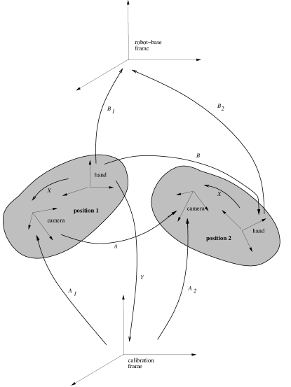
Figure 1: A general view showing two different positions of the hand-eye device. One is interested to estimate matrix $X$ or, alternatively, matrix $Y$ (see text).

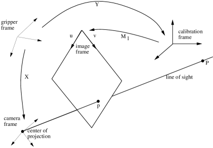
Figure 2: The line of sight passing through the center of projection and the image point $p$ may well be expressed in the calibration frame, using the coefficients of the perspective matrix $M_{1}$.

2.2 The new formulation

The previous formulation implies that the camera is calibrated at each different position $i$ of the hand-eye device. Once the camera is calibrated, its extrinsic parameters, namely the matrix $A_{i}$ for position $i$, are made explicit. This is done by decomposing the 3$\times$4 perspective matrix $M_{i}$, that is obtained by calibration, into intrinsic and extrinsic parameters (Faugeras and Toscani, 1986), (Tsai, 1987), (Horaud and Monga, 1993):

$$M_{i} = CA_{i}$$ (10)

$$= \left(\begin{array}[]{cccc}\alpha_{u}&0&u_{0}&0\\ 0&\alpha_{v}&v_{0}&0\\ 0&0&1&0\end{array}\right)\left(\begin{array}[]{cc}R_{A}^{i}&t_{A}^{i}\\ 0&1\end{array}\right)$$

The parameters $\alpha_{u}$, $\alpha_{v}$, $u_{0}$ and $v_{0}$ describe the affine transformation between the camera frame and the image frame. This decomposition assumes that the camera is described by a pin-hole model and that the optical axis associated with this model is perpendicular to the image plane.

The new formulation that we present here avoids the above decomposition. Let $Y$ be the transformation matrix from the hand frame to the calibration frame, when the hand-eye device is in position 1. Clearly we have, e.g., Figure 1:

$$X=A_{1}Y$$ (11)

Therefore matrix $Y$ is equivalent to matrix $X$, up to a rigid transformation $A_{1}$. By substituting $X$ given by this last equation and $A$ given by eq. (3) into eq. (1), we obtain:

$$A_{2}Y=A_{1}YB$$

By pre multiplying the terms of this equality with matrix $C$ and using eq. (10) with $i=1,2$ we obtain:

$$M_{2}Y=M_{1}YB$$ (12)

which is equivalent to eq. (2).

In this equation the unknown $Y$ is the transformation from the hand frame to the calibration frame, e.g., Figure 1. The latter frame may well be viewed as the camera frame provided that the 3$\times$4 perspective matrix $M_{1}$ is known. Mathematically, choosing the calibration frame rather then the camera frame is equivalent to replacing the 3$\times$4 perspective matrix $C$ with the more general matrix $M_{1}$. The advantage of using $M_{1}$ rather than $C$ is that one has not to assume a perfect pin hole camera model anymore. Therefore, problems due to the decomposition of $M_{1}$ into external and internal camera parameters, i.e., $M_{i}=CA_{i}$, will disappear.

Referring to Figure 2, the projection of a point $P$ onto the image is described by:

$$\left(\begin{array}[]{l}su\\ sv\\ s\end{array}\right)=M_{1}\left(\begin{array}[]{l}x\\ y\\ z\\ 1\end{array}\right)$$ (13)

or:

$$u=\frac{m_{11}x+m_{12}y+m_{13}z+m_{14}}{m_{31}x+m_{32}y+m_{33}z+m_{34}}$$ (14)

$$v=\frac{m_{21}x+m_{22}y+m_{23}z+m_{24}}{m_{31}x+m_{32}y+m_{33}z+m_{34}}$$ (15)

where $x$, $y$, and $z$ are the coordinates of $P$ in the calibration frame, $u$ and $v$ are the image coordinates of $p$–the projection of $P$, and the $m_{ij}$’s are the coefficients of $M_{1}$. Notice that these two equations can be rewritten as:

$$(m_{11}-um_{31}) \;x+(m_{12}-um_{32})\;y$$

$$+(m_{13}-um_{33})\;z=um_{34}-m_{14}$$ (16)

$$(m_{21}-vm_{31}) \;x+(m_{22}-vm_{32})\;y$$

$$+(m_{23}-vm_{33})\;z=vm_{34}-m_{24}$$ (17)

These equations may be interpreted as follows. Given a matrix $M_{1}$ and an image point $p$, eq. (2.2) and eq. (2.2) describe a line of sight passing through the center of projection and through $p$. This line is given in the calibration frame which may well be viewed as the camera frame.

The determination of the hand-eye geometry (matrix $X$ in the classical formulation or matrix $Y$ in our new formulation) allows one to express any line of sight associated with an image point $p$ in the hand frame and hence, in any robot centered frame.

2.3 Summary

In practice, the classical and the new formulations summarize as follows. Let $n$ be the number of different positions of the hand-eye device with respect to a fixed calibration frame. We have:

1. Classical formulation. The matrix $X$ is the solution of the following set of $n-1$ matrix equations:

   $$\left\{\begin{array}[]{ccc}A_{12}X&=&XB_{12}\\ &\vdots&\\ A_{i-1\;i}X&=&XB_{i-1\;i}\\ &\vdots&\\ A_{n-1\;n}X&=&XB_{n-1\;n}\end{array}\right.$$ (18)

   where $A_{i-1\;i}$ denotes the transformation between position $i-1$ and position $i$ of the camera frame and $B_{i-1\;i}$ denotes the transformation between position $i-1$ and position $i$ of the hand frame.

2. New formulation. The matrix $Y$ is the solution of the following set of $n-1$ matrix equations:

   $$\left\{\begin{array}[]{ccc}M_{2}Y&=&M_{1}YB_{12}\\ &\vdots&\\ M_{i}Y&=&M_{1}YB_{1i}\\ &\vdots&\\ M_{n}Y&=&M_{1}YB_{1n}\end{array}\right.$$ (19)

   where $M_{i}$ is the projective transformation between the calibration frame and the camera frame in position $i$ and $B_{1i}$ denotes the transformation between position 1 and position $i$ of the hand frame.

3 Previous approaches

Previous approaches for solving the hand-eye calibration problem attempted to solve eq. (1) ($AX=XB$) by farther decomposing it into two equations: A matrix equation depending on rotation and a vector equation depending both on rotation and translation:

$$R_{A}R_{X}=R_{X}R_{B}$$ (20)

and:

$$(R_{A}-I)t_{X}=R_{X}t_{B}-t_{A}$$ (21)

In this equation $I$ is the 3$\times$3 identity matrix.

In order to solve eq. (20) one may take advantage of the particular algebraic and geometric properties of rotation (orthogonal) matrices. Indeed this equation can be written as:

$$R_{A}=R_{X}R_{B}R_{X}^{T}$$ (22)

which is a similarity transformation since $R_{X}$ is an orthogonal matrix. Hence, matrices $R_{A}$ and $R_{B}$ have the same eigenvalues. A well-known property of a rotation matrix is that is has one of its eigenvalues equal to 1. Let $n_{B}$ be the eigenvector of $R_{B}$ associated with this eigenvalue. By post multiplying eq. (20) with $n_{B}$ we obtain:

$$R_{A}R_{X}n_{B}=R_{X}R_{B}n_{B}=R_{X}n_{B}$$

and we conclude that $R_{X}n_{B}$ is equal to $n_{A}$, the eigenvector of $R_{A}$ associated with the unit eigenvalue:

$$n_{A}=R_{X}n_{B}$$ (23)

To conclude, solving for $AX=XB$ is equivalent to solving for eq. (23) and for eq. (21). Solutions were proposed, among others, by (Shiu and Ahmad, 1989), (Tsai and Lenz, 1989), (Chou and Kamel, 1991), and (Wang, 1992). All these authors noticed that at least three positions are necessary in order to uniquely determine $X$, i.e., $R_{X}$ and $t_{X}$. (Shiu and Ahmad, 1989) cast the rotation determination problem into the problem of solving for 8 linear equations in 4 unknowns and they used standard linear algebra techniques in order to obtain a solution.

(Tsai and Lenz, 1989) suggested to represent $R_{X}$ by its unit eigenvector $n_{X}$ and an angle $\theta_{X}$. They noticed that:

$$n_{X}\cdot(n_{A}-n_{B})=0$$

and

$$(n_{A}-n_{B})\cdot(n_{A}+n_{B})=0$$

These expressions allow one to cast eq. (23) into:

$$(n_{A}+n_{B})\times n=n_{A}-n_{B}$$ (24)

with:

$$n=\left(\tan\frac{\theta_{X}}{2}\right)n_{X}$$

It is easy to notice that eq. (24) is rank deficient and hence, at least two independent hand-eye motions (at least three positions) are necessary for determining a unique solution. In the general case of $n$ motions ($n+1$ positions of the hand-eye device relative to the calibration frame) one may solve for an over constrained set of $2n$ linear equations in 3 unknowns.

(Chou and Kamel, 1991) suggested to represent rotation by a unit quaternion and they used the singular value decomposition method in order to solve for the linear algebra. The idea of using a unit quaternion is a good one. Unfortunately the authors were not aware of the closed-form solution that is available in conjunction with unit quaternions for determining rotation optimally as it was proposed both by (Horn, 1987) and by (Faugeras and Hebert, 1986).

(Wang, 1992) suggested three methods that roughly correspond to the solution proposed by (Tsai and Lenz, 1989). Then he compared his best method to the methods proposed by (Shiu and Ahmad, 1989) and by (Tsai and Lenz, 1989). The conclusions of his comparison are that the (Tsai and Lenz, 1989) method yield the best results.

(Chen, 1991) showed that the hand-eye geometry can be conveniently described using a screw representation for rotation and translation. This representation allows a uniqueness analysis.

All these approaches have the following features in common:

• rotation is decoupled from translation;

• the solution for rotation is estimated using linear algebra techniques;

• the solution for translation is estimated using linear algebra as well.

Decoupling rotation and translation is certainly a good idea. It leads to simple numerical solutions. However, in the presence of errors the linear problem to be solved becomes ill-conditioned and the solution available with the linear system is not valid. This is due to the fact that the geometric properties allowing the linearization of the rotation equation do not hold in the presence of noise. Errors may be due both to camera calibration inaccuracies and to inexact knowledge of the robot’s kinematic parameters.

4 Decomposing the new formulation

In this section we show that the new formulation that we introduced in section 2.2 has a mathematical structure that is identical to the classical formulation. This will allow us to formulate a unified approach that solves for either of the two formulations.

We start by making explicit the 3$\times$4 perspective matrix $M$ as a function of intrinsic and extrinsic parameters, i.e., eq. (10):

$$M=\left(\begin{matrix}\alpha_{u}r_{11}+u_{0}r_{31}&\alpha_{u}r_{12}+u_{0}r_{32}\\ \alpha_{v}r_{21}+v_{0}r_{31}&\alpha_{v}r_{22}+v_{0}r_{32}\\ r_{31}&r_{32}\end{matrix}\right.\\ \left.\begin{matrix}\alpha_{u}r_{13}+u_{0}r_{33}&\alpha_{u}t_{x}+u_{0}t_{z}\\ \alpha_{v}r_{23}+v_{0}r_{33}&\alpha_{v}t_{y}+v_{0}t_{z}\\ r_{33}&t_{z}\end{matrix}\right)$$

Notice that a matrix $M_{i}$ of this form can be written as:

$$M_{i}=\left(\begin{array}[]{cc}N_{i}&n_{i}\end{array}\right)$$

where $N_{i}$ is a 3$\times$3 matrix and $n_{i}$ is a 3-vector. One may notice that in the general case $N_{i}$ has an inverse since the vectors $(r_{11}\;r_{12}\;r_{13})^{T}$, $(r_{21}\;r_{22}\;r_{23})^{T}$, and $(r_{31}\;r_{32}\;r_{33})^{T}$ are mutually orthogonal and $\alpha_{u}\neq 0$, $\alpha_{v}\neq 0$. With this notation eq. (12) may be decomposed into a matrix equation:

$$N_{2}R_{Y}=N_{1}R_{Y}R_{B}$$ (25)

and a vector equation:

$$N_{2}t_{Y}+n_{2}=N_{1}R_{Y}t_{B}+N_{1}t_{Y}+n_{1}$$ (26)

Introducing the notation:

$$N=N_{1}^{-1}N_{2}$$

eq. (25) becomes:

$$NR_{Y}=R_{Y}R_{B}$$ (27)

or:

$$N=R_{Y}R_{B}R_{Y}^{T}$$

Two properties of $N$ may be easily derived:

1. $N$ is the product of three rotation matrices, it is therefore a rotation itself and:

   $$N^{-1}=N^{T}$$

2. Since $R_{Y}$ is an orthogonal matrix, the above equation defines a similarity transformation. It follows that $N$ has the same eigenvalues as $R_{B}$. In particular $R_{B}$ has an eigenvalue equal to 1 and let $n_{B}$ be the eigenvector associated with this eigenvalue.

If we denote by $n_{N}$ the eigenvector of $N$ associated with the unit eigenvalue, then we obtain:

$$NR_{Y}n_{B} = R_{Y}R_{B}n_{B}$$

$$= R_{Y}n_{B}$$

and hence we have:

$$n_{N}=R_{Y}n_{B}$$ (28)

This equation is identical to eq. (23) in the classical formulation.

By premultiplying eq. (26) with $N_{1}^{-1}$ we obtain:

$$(N-I)t_{Y}=R_{Y}t_{B}-t_{N}$$ (29)

with:

$$t_{N}=N_{1}^{-1}(n_{2}-n_{1})$$

and one may easily notice that this equation is identical to eq. (21) in the classical formulation.

To conclude, the classical formulation decomposes in eq. (23) and in eq. (21) and, equivalently, the new formulation decomposes in eq. (28) and eq. (29).

5 A unified optimal solution

In the previous sections we showed that the classical and the new formulations are mathematically equivalent. Indeed, the classical formulation, $AX=XB$ decomposes into eqs. (23) and (21):

$$n_{A} = R_{X}n_{B}$$

$$(R_{A}-I)t_{X} = R_{X}t_{B}-t_{A}$$

and the new formulation, $MY=M^{\prime}YB$ decomposes into eqs. (28) and (29):

$$n_{N} = R_{Y}n_{B}$$

$$(N-I)t_{Y} = R_{Y}t_{B}-t_{N}$$

These two sets of equations are of the form:

$$v^{\prime}=Rv$$ (30)

$$(K-I)t=Rp-p^{\prime}$$ (31)

where $R$ and $t$ are the parameters to be estimated (rotation and translation), $v^{\prime}$, $v$, $p^{\prime}$, $p$ are 3-vectors, $K$ is a 3$\times$3 orthogonal matrix and $I$ is the identity matrix.

Eqs. (30) and (31) are associated with one motion of the hand-eye device. In order to estimate $R$ and $t$ at least two such motions are necessary. In the general case of $n$ motions one may cast the problem of solving 2$n$ such equations into the problem of minimizing two positive error functions:

$$f_{1}(R)=\sum_{i=1}^{n}\|v^{\prime}_{i}-Rv_{i}\|^{2}$$ (32)

and

$$f_{2}(R,t)=\sum_{i=1}^{n}\|Rp_{i}-(K_{i}-I)t-p^{\prime}_{i}\|^{2}$$ (33)

Therefore, two approaches are possible:

1. $R$ then $t$. Rotation is estimated first by minimizing $f_{1}$. This minimization problem has a simple closed-form solution that will be detailed below. Once the optimal rotation is determined, the minimization of $f_{2}$ over the translational parameters is a linear least-squared problem.

2. $R$ and $t$. Rotation and translation are estimated simultaneously by minimizing $f_{1}+f_{2}$. This minimization problem is non-linear but, as it will be shown below, it provides the most stable solution.

5.1 Rotation then translation

In order to minimize $f_{1}$ given by eq. (32) we represent rotation by a unit quaternion. With this representation one may write, (see Appendix A, eq. (A)):

$$Rv_{i}=q\ast v_{i}\ast\overline{q}$$

Moreover, using eq. (38), one may successively write:

$$\|v^{\prime}_{i}- q\ast v_{i}\ast\overline{q}\|^{2}=\|v^{\prime}_{i}-q\ast v_{i}\ast\overline{q}\|^{2}\|q\|^{2}$$

$$= \|v^{\prime}_{i}\ast q-q\ast v_{i}\|^{2}$$

$$= (Q(v^{\prime}_{i})q-W(v_{i})q)^{T}(Q(v^{\prime}_{i})q-W(v_{i})q)$$

$$= q^{T}{\cal{A}}_{i}q$$

with ${\cal{A}}_{i}$ being a 4$\times$4 positive symmetric matrix:

$${\cal{A}}_{i}=(Q(v^{\prime}_{i})-W(v_{i}))^{T}(Q(v^{\prime}_{i})-W(v_{i}))$$

Finally the error function becomes:

$$f_{1}(R) = f_{1}(q)$$

$$= \sum_{i=1}^{n}\|v^{\prime}_{i}-q\ast v_{i}\ast\overline{q}\|^{2}$$

$$= \sum_{i=1}^{n}q^{T}{\cal{A}}_{i}q$$

$$= q^{T}\left(\sum_{i=1}^{n}{\cal{A}}_{i}\right)q$$

$$= q^{T}{\cal{A}}q$$

with ${\cal{A}}=\sum_{i=1}^{n}{\cal{A}}_{i}$ and one has to minimize $f_{1}$ under the constraint that $q$ must be a unit quaternion. This constrained minimization problem can be solved using the Lagrange multiplier:

$$\min_{q}f_{1}=\min_{q}(q^{T}{\cal{A}}q+\lambda(1-q^{T}q))$$

By differentiating this error function with respect to $q$ one may easily find the solution in closed form:

$${\cal{A}}q=\lambda q$$

The unit quaternion minimizing $f_{1}$ is therefore the eigenvector of ${\cal{A}}$ associated with its smallest (positive) eigenvalue. This closed-form solution was introduced by (Faugeras and Hebert, 1986) for finding the best rotation between two sets of 3-D features.

Once the rotation has been determined, the problem of determining the best translation becomes a linear least-squares problem that can be easily solved using standard linear algebra techniques.

5.2 Rotation and translation

The problem of estimating rotation and translation simultaneously can be stated in terms of the following minimization problem:

$$\min_{q,t}(f_{1}+f_{2})$$

We have been unable to solve this problem in closed form. One may notice that the error function to be minimized is a sum of squares of non linear functions. Because of the special structure of the Jacobian and Hessian matrices associated with error functions of this type, a number of special minimization methods have been designed specifically to deal with this case, (Gill et al, 1989). Among these methods, the Levenberg-Marquardt method and the trust-region method (Fletcher, 1990), (Phong et al, 1993a), (Phong et al, 1993b) are good candidates.

Using unit quaternions the error function to be minimized is:

$$\min_{q,t}(f(q,t)+\lambda(1-q^{T}q)^{2})$$ (35)

with:

$$f(q,t) = \lambda_{1}f_{1}(q)+\lambda_{2}f_{2}(q,t)$$

$$= \lambda_{1}\sum_{i=1}^{n}\|v^{\prime}_{i}-q\ast v_{i}\ast\overline{q}\|^{2}$$

$$+ \lambda_{2}\sum_{i=1}^{n}\|q\ast p_{i}\ast\overline{q}-(K_{i}-I)t-p^{\prime}_{i}\|^{2}$$

which has the form of sum of squares of non linear functions and $\lambda(1-q^{T}q)^{2}$ is a penalty function that guarantees that $q$ (a quaternion) has a module equal to 1. $\lambda_{1}$ and $\lambda_{2}$ are two weights and $\lambda$ is a real positive number. High values for $\lambda$ insure that the module of $q$ is closed to 1. In all our experiments we have:

$$\lambda_{1}=\lambda_{2}=1$$

$$\lambda=2\times 10^{6}$$

There are two possibilities for solving the non linear minimization problem of equation (35). The first possibility is to consider it as a classical non linear least squares minimization problem and to apply standard non linear optimization techniques, such as Newton’s method and Newton-like methods (Gill et al, 1989), (Fletcher, 1990). In the next two sections we give some results obtained with the Levenberg-Marquardt non linear minimization method as described in (Press et al, 1988).

The second possibility is to try to simplify the expression of the error function to be minimized. Using properties associated with quaternions, the error function may indeed be simplified. We already obtained a simple analytic form for $f_{1}$, i.e., eq. (5.1). Similarly, $f_{2}$ simplifies as well.

Indeed, $f_{2}$ is the sum of terms such as:

$$\|q\ast p_{i}\ast\overline{q}-(K_{i}-I)t-p^{\prime}_{i}\|^{2}$$

and we have:

$$\|q\ast p_{i}\ast\overline{q} -(K_{i}-I)t-p^{\prime}_{i}\|^{2}\|q\|^{2}$$

$$=\|q\ast p_{i}-(K_{i}-I)t\ast q-p^{\prime}_{i}\ast q\|^{2}$$

Using the matrix representation for quaternion multiplication one can easily obtain (see Appendix B for the derivation of this equation):

$$f_{2}(q,t) =q^{T}(\sum_{i=1}^{n}{\cal{B}}_{i})q+t^{T}(\sum_{i=1}^{n}{\cal{C}}_{i})t+(\sum_{i=1}^{n}\delta_{i})t$$

$$+(\sum_{i=1}^{n}\varepsilon_{i})Q(q)^{T}W(q)t$$ (36)

The 4$\times$4 matrices ${\cal{B}}_{i}$ and ${\cal{C}}_{i}$, and the 1$\times$4 vectors $\delta_{i}$ and $\varepsilon_{i}$ are:

$${\cal{B}}_{i} = (p_{i}^{T}p_{i}+p_{i}^{\prime T}p_{i}^{\prime})I-W(p_{i})^{T}Q(p_{i}^{\prime})-Q(p_{i}^{\prime})^{T}W(p_{i})$$

$${\cal{C}}_{i} = K_{i}^{T}K_{i}-K_{i}-K_{i}^{T}+I$$

$$\delta_{i} = 2p_{i}^{\prime T}(K_{i}-I)$$

$$\varepsilon_{i} = -2p_{i}^{T}(R_{B_{i}}-I)$$

With the notations: ${\cal{B}}=\sum_{i=1}^{n}{\cal{B}}_{i}$, ${\cal{C}}=\sum_{i=1}^{n}{\cal{C}}_{i}$, $\delta=\sum_{i=1}^{n}\delta_{i}$, $\varepsilon=\sum_{i=1}^{n}\varepsilon_{i}$, and with ${\cal{A}}$ already defined, we obtain the following non linear minimization problem:

$$\min_{q,t}(q^{T}({\cal{A}}+{\cal{B}})q+t^{T}{\cal{C}}t+\delta t+\varepsilon Q(q)^{T}W(q)t+\\ \lambda(1-q^{T}q)^{2})$$ (37)

which is the sum of 5 terms. The number of parameters to be estimated is 7 (4 for the unit quaternion and 3 for the translation). It is worthwhile to notice that the number of terms of this error function is constant with respect to $n$, i.e., the number of hand-eye motions. For such minimization problems one may use constrained step methods such as the trust region method (Fletcher, 1990), (Yassine, 1989).

6 Stability analysis and method comparison

One of the most important merits of any hand-eye calibration method is its stability with respect to various perturbations. There are two main sources of perturbations: errors associated with camera calibration and errors associated with the robot motion. Indeed, the parameters of both the direct and inverse kinematic models of robots are not perfect. As a consequence the real motions associated with both the hand and the camera are known up to some uncertainty. It follows that the estimation of the hand-eye transformation has errors associated with it and it is important to quantify these errors in order to determine the stability of a given method and to compare various methods.

In order to perform this stability analysis we designed a stability analysis based on the following grounds:

• Nominal values for the parameters of the hand-eye transformation ($X$ or $Y$) are provided;

• Also are provided $n+1$ matrices $A_{1}$, …$A_{n+1}$ from which $n$ hand motions can be computed either with (see Section 2):

  $$B_{ii+1}=X^{-1}A_{i+1}A_{i}^{-1}X$$

  or with:

  $$B_{1i}=Y^{-1}A_{1}^{-1}A_{i}Y$$

• Gaussian noise or uniform noise is added to both the camera and hand motions and $X$ (or $Y$) is estimated in the presence of this noise using three different methods: Tsai-Lenz, closed-form solution, and non-linear optimization, and

• We study the variations of the estimation of the hand-eye transformation as a function of the noise being added and/or as a function of the number of motions ($n$).

Since both rotations and translations may be represented as vectors, adding noise to a transformation consists of adding random numbers to each one of the vectors’ components. Random numbers simulating noise are obtained using a random number generator either with a uniform distribution in the interval $[-C/2,+C/2]$, or with a Gaussian distribution with a standard deviation equal to $\sigma$. Therefore the level of noise that is added is associated either with the value of $C$ or with the value of $\sigma$ (or, more precisely, with the value of 2$\sigma$). In what follows the level of noise is in fact represented as a ratio: the values of the actual random numbers divided by the values of the perturbed parameters.

In the case of a rotation, the vector associated with this rotation has a module equal to 1 and therefore the ratio is simply either $C$ or 2$\sigma$. In the case of a translation the ratio is computed with respect to a nominal value estimated over all the perturbed translations:

$$\|t_{nominal}\|=\frac{\sum_{i=1}^{n}(\|t_{A_{ii+1}}\|+\|t_{B_{ii+1}}\|)}{2n}$$

where $t_{A_{ii+1}}$ is the translation vector associated with $A_{ii+1}$.

For each noise level and for a large number $J$ of trials we compute the errors associated with rotation and translation as follows:

$$e_{rot}=\sqrt{\frac{1}{J}\sum_{j=1}^{J}\|\tilde{R}_{j}-R\|^{2}}$$

and:

$$e_{tr}=\frac{\sqrt{\frac{1}{J}\sum_{j=1}^{J}\|\tilde{t}_{j}-t\|^{2}}}{\|t\|}$$

where $R$ and $t$ are the nominal values of the transformation being estimated ($X$ or $Y$), $\tilde{R}_{j}$ and $\tilde{t}_{j}$ are the estimated rotation and translation for some trial $j$, and $J$ is the number of trials for each noise level (defined either by $C$ or by $\sigma$). In all our experiments we set $J=1000$ and $\|t\|=157$mm.

Figure 3: Error in rotation in the presence of uniform noise perturbing the rotation axes.

Figure 4: Error in translation in the presence of uniform noise perturbing the rotation axes.

Figure 5: Error in rotation in the presence of uniform noise perturbing the translation vectors and the rotation axes.

Figure 6: Error in translation in the presence of uniform noise perturbing the translation vectors and the rotation axes.

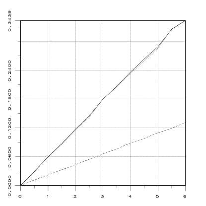
Figure 7: Error in rotation in the presence of Gaussian noise perturbing the rotation axes.

Figure 8: Error in translation in the presence of Gaussian noise perturbing the rotation axes.

Figure 9: Error in rotation in the presence of Gaussian noise perturbing the translation vectors and the rotation axes.

Figure 10: Error in translation in the presence of Gaussian noise perturbing the translation vectors and the rotation axes.

Figure 11: Error in rotation as a function of the number of motions.

Figure 12: Error in translation as a function of the number of motions.

The following figures show the above errors as a function of the percentage of noise. The percentage of noise varies from 1% to 6%. The full curves (—) correspond to the method of Tsai & Lenz, the dotted curves ( …) correspond to the closed-form method and the dashed curves (- - -) correspond to the non-linear method. Figure 3 through Figure 10 correspond to two motions ($n=2$) of the hand-eye device while on Figure 11 and Figure 12 the number of motions varies from 2 to 9.

Figure 3 and Figure 4 show the rotation and translation errors as a function of uniform noise added to the rotational part of the hand and camera motions. Figure 5 and Figure 6 show the rotation and translation errors as a function of uniform noise added both to the rotational and translational parts of the camera and hand motions. Figure 7 through Figure 10 are similar to Figure 3 through Figure 6 but the uniform distribution of the noise has been replaced by a Gaussian distribution.

It is interesting to notice that the Tsai-Lenz method and closed-form method have almost the same behaviour while the non-linear method provides more accurate results in all the situations. The fact that the results obtained with the first two methods are highly correlated may be due to the fact that both these methods decouple the estimation of rotation from the estimation of translation. This behaviour seems to be independent with respect to the noise type (uniform or Gaussian) and of whether only rotation is perturbed or rotation and translation are perturbed simultaneously. We conclude that the decoupling of rotation and translation introduces a bias in the estimation of the hand-eye transformation.

As other authors have done in the past, it is interesting to analyse the behaviour of hand-eye calibration with respect to the number of motions. In order to perform this analysis we have to fix the percentage of noise. Figure 11 and Figure 12 show the rotational and translational errors as a function of the squared root of the number of motions ($\sqrt{n}$ varies from $1.414$ to $3$). The noise ratio has been fixed to the worst case for rotations, e.g., 6% and to 2% for translations. Both rotational and translational noise distributions are Gaussian. For example, for 4 motions the error in translation is of 4% for the non-linear method and of 6.5% for the other two methods.

7 Experimental results

$AX=XB$	$\sum\|R_{A}R_{X}-R_{X}R_{B}\|^{2}$	$\frac{\sum\|(R_{A}-I)t_{X}-R_{X}t_{B}+t_{A}\|^{2}}{\sum\|R_{X}t_{B}-t_{A}\|^{2}}$
Tsai-Lenz	0.0006	0.032
Closed-form solution	0.0005	0.029
Non-linear optimization	0.0003	0.019

Table 1: The classical formulation used with the first data set.

$AX=XB$	$\sum\|R_{A}R_{X}-R_{X}R_{B}\|^{2}$	$\frac{\sum\|(R_{A}-I)t_{X}-R_{X}t_{B}+t_{A}\|^{2}}{\sum\|R_{X}t_{B}-t_{A}\|^{2}}$
Tsai-Lenz	0.0014	0.036
Closed-form solution	0.0014	0.023
Non-linear optimization	0.0017	0.015
$MY=M^{\prime}YB$	$\sum\|NR_{Y}-R_{Y}R_{B}\|^{2}$	$\frac{\sum\|(N-I)t_{Y}-R_{Y}t_{B}+t_{N}\|^{2}}{\sum\|R_{Y}t_{B}-t_{N}\|^{2}}$
Tsai-Lenz	0.0031	0.0021
Closed-form solution	0.0015	0.001
Non-linear optimization	0.0013	0.0006

Table 2: The classical and the new formulations used with the second data set.

$AX=XB$	$\sum\|R_{A}R_{X}-R_{X}R_{B}\|^{2}$	$\frac{\sum\|(R_{A}-I)t_{X}-R_{X}t_{B}+t_{A}\|^{2}}{\sum\|R_{X}t_{B}-t_{A}\|^{2}}$	CPU time
Tsai-Lenz	0.014	0.23	0.08
Closed-form solution	0.036	0.223	0.06
Non-linear optimization	0.258	0.058	0.21
$MY=M^{\prime}YB$	$\sum\|NR_{Y}-R_{Y}R_{B}\|^{2}$	$\frac{\sum\|(N-I)t_{Y}-R_{Y}t_{B}+t_{N}\|^{2}}{\sum\|R_{Y}t_{B}-t_{N}\|^{2}}$
Tsai-Lenz	0.038	0.039	0.06
Closed-form solution	0.035	0.037	0.08
Non-linear optimization	0.04	0.034	0.25

Table 3: The classical and the new formulations used with the third data set. The last column indicates the CPU time in seconds on a Sparc-10 Sun computer.

In this section we report some experimental results obtained with three sets of data. The first data set was provided by François Chaumette from IRISA and the second and third data sets were obtained at LIFIA. The first data set was obtained with 17 different positions of the hand-eye device with respect to a calibrating object. The second data set was obtained with 7 such positions. The third data set was obtained with 6 positions. For the first set only the extrinsic camera parameters were provided while for the latter sets we had access to the full 3$\times$4 perspective matrices. Therefore, the latter sets allowed us to test both the classical and the new formulations. The only restrictions imposed onto the robot motions are due to the fact that in eachone of its positions the camera mounted onto the robot must see the calibration pattern.

In order to calibrate the camera we used the method proposed by Faugeras & Toscani (Faugeras and Toscani, 1986) and the following setup. The calibrating pattern consists of a planar grid of size 200$\times$300mm that can move along an axis perpendicular to its plane. The distance from this calibrating grid to the camera varies during hand-eye calibration between 600mm and 1000mm. This calibration setup combined with the Faugeras-Toscani method provides very accurate camera calibration data. This is mainly due to the accuracy of the grid points (0.1mm), to the accuracy of point localization in the image (0.1 pixels), and to the large number of calibrating points being used (460 points). Moreover, camera calibration errors can be neglected with respect to robot calibration errors (see below).

Since the two formulations are mathematically equivalent, we have been able to test and compare the classical Tsai-Lenz method with the two methods developed in this paper. Table 1, Table 2, and Table 3 summarize the results obtained with the three data sets mentioned above. The lengths of the translation vectors thus obtained are: $\|t_{X}\|=93$mm and $\|t_{Y}\|=681$mm.

The second columns of these tables show the sum of squares of the absolute error in rotation. The third columns show the sum of squares of the relative error in translation.

These experimental results seem to confirm that, on one hand, the non-linear method provides a better estimation of the translation vector – at the cost of a, sometimes, slightly less accurate rotation – and, on the other hand, the new formulation provides a better estimation of the transformation parameters than the classical formulation.

It is worthwhile to notice that, while the non-linear technique provides the most accurate results with simulated data, the linear and closed-form techniques provide sometimes a better estimation of rotation with real data. This is due to the fact that the robot’s kinematic chain is not perfectly calibrated and therefore there are errors associated with the robot’s translation parameters. Obviously, these errors do not obey the noise models used for simulations. The linear and closed-form techniques estimate the rotation parameters independently of the robot’s translation parameters and therefore the rotation thus estimated is not affected by translation errors. However, in practice we prefer the non-linear technique.

8 Discussion

In this paper we attacked the problem of hand-eye calibration. In addition to the classical formulation, i.e., $AX=XB$, we suggest a new formulation that directly uses the 3$\times$4 perspective matrices available with camera calibration: $MY=M^{\prime}YB$. The advantage of the new formulation with respect to the classical one is that it avoids the decomposition of the perspective matrix into intrinsic and extrinsic camera parameters. Indeed, it has long been recognised in computer vision research that this decomposition is unstable.

Moreover, we show that the new formulation has a mathematical structure that is identical with the mathematical structure of the classical formulation. The advantage of this mathematical analogy is that, the two formulations being variations of the same one, any method for solving the problem applies to both formulations.

We develop two resolution methods, the first one solves for rotation and then for translation while the second one solves simultaneously for rotation and translation. Using unit quaternions to represent rotations, the first method leads to a closed form solution introduced by Faugeras & Hebert (Faugeras and Hebert, 1986) while the second one is new and leads to non-linear optimization. Among the many robust non-linear optimization methods that are available, we chose the Levenberg-Marquardt technique.

Both the stability analysis and the results obtained with experimental data from two laboratories show that the non-linear optimization method yields the most accurate results. Linear algebra techniques (the Tsai-Lenz method) and the closed-form method (using unit quaternions) are of comparable accuracy.

The new formulation provides much more accurate hand-eye calibration results than the classical formulation. This improvement in accuracy seems to confirm that the decomposition of the perspective matrix into intrinsic and extrinsic parameters introduces some errors. Nevertheless, the intrinsic parameters, even if they don’t need to be made explicit, are assumed to be constant during calibration. We are perfectly aware that this assumption is not very realistic and may cause problems in practice. We are currently investigating ways to give up this assumption.

Also, we investigate ways to perform hand-eye calibration and robot calibration simultaneously. Indeed, in many applications such as nuclear and space environments it may be useful to calibrate a robot simply by calibrating a camera mounted onto the robot.

Appendix A Rotation and unit quaternion

The use of unit quaternions to represent rotations is justified by an elegant closed-form solution associated with the problem of optimally estimating rotation from 3-D to 3-D vector correspondences (Faugeras and Hebert, 1986), (Horn, 1987), (Sabata and Aggarwal, 1991), (Horaud and Monga, 1993). In section 5 we stressed the similarity between the hand-eye calibration problem and the problem of optimally estimating the rotation between sets of 3-D features. In this appendix we briefly recall the definition of quaternions, some useful properties of the quaternion multiplication operator, and the relationship between 3$\times$3 orthogonal matrices and unit quaternions.

A quaternion is a 4-vector that may be viewed as a special case of complex numbers that have one real part and three imaginary parts:

$$q=q_{0}+iq_{x}+jq_{y}+kq_{z}$$

with:

$$i^{2}=j^{2}=k^{2}=ijk=-1$$

One may define quaternion multiplication (denoted by $\ast$) as follows:

$$r\ast q=(r_{0}+ir_{x}+jr_{y}+kr_{z})(q_{0}+iq_{x}+jq_{y}+kq_{z})$$

which can be written using a matrix notation:

$$r\ast q=Q(r)q=W(q)r$$

with:

$$Q(r)=\left(\begin{array}[]{rrrr}r_{0}&-r_{x}&-r_{y}&-r_{z}\\ r_{x}&r_{0}&-r_{z}&r_{y}\\ r_{y}&r_{z}&r_{0}&-r_{x}\\ r_{z}&-r_{y}&r_{x}&r_{0}\end{array}\right)$$

and:

$$W(r)=\left(\begin{array}[]{rrrr}r_{0}&-r_{x}&-r_{y}&-r_{z}\\ r_{x}&r_{0}&r_{z}&-r_{y}\\ r_{y}&-r_{z}&r_{0}&r_{x}\\ r_{z}&r_{y}&-r_{x}&r_{0}\end{array}\right)$$

One may easily verify the following properties:

$$Q(r)^{T}Q(r) =Q(r)Q(r)^{T}=r^{T}rI$$

$$W(r)^{T}W(r) =W(r)W(r)^{T}=r^{T}rI$$

$$Q(r)q =W(q)r$$

$$Q(r)^{T}r =W(r)^{T}r=r^{T}re$$

$$Q(r)Q(q) =Q(Q(r)q)$$

$$W(r)W(q) =W(W(r)q)$$

$$Q(r)W(q)^{T} =W(q)^{T}Q(r)$$

$e$ being the unity quaternion: $e=(1\;0\;0\;0)$.

The dot-product of two quaternions is:

$$r\cdot q=r_{0}q_{0}+r_{x}q_{x}+r_{y}q_{y}+r_{z}q_{z}$$

The conjugate quaternion of $q$, $\overline{q}$ is defined by:

$$\overline{q}=q_{0}-iq_{x}-jq_{y}-kq_{z}$$

and obviously we have:

$$q\ast\overline{q}=q\cdot q=\|q\|^{2}$$

An interesting property that is straightforward and which will be used in the next section is:

$$\|r\ast q\|^{2}=\|r\|^{2}\|q\|^{2}$$ (38)

A 3-vector may well be viewed as a purely imaginary quaternion (its real part is equal to zero). One may notice that $W(v)$ and $Q(v)$ associated with a 3-vector $v$ are skew-symmetric matrices.

Let $q$ be a unit quaternion, that is $q\cdot q=1$, and let $v$ be a purely imaginary quaternion. We have:

$$v^{\prime} = q\ast v\ast\overline{q}$$

$$= (Q(q)v)\ast\overline{q}$$

$$= (W(q)^{T}Q(q))v$$

and one may easily figure out that:

$$W(q)^{T}Q(q)=\left(\begin{matrix}1&0\\ 0&q_{0}^{2}+q_{x}^{2}-q_{y}^{2}-q_{z}^{2}\\ 0&2(q_{x}q_{y}+q_{0}q_{z})\\ 0&2(q_{x}q_{z}-q_{0}q_{y})\end{matrix}\right.\\ \left.\begin{matrix}0&0\\ 2(q_{x}q_{y}-q_{0}q_{z})&2(q_{x}q_{z}+q_{0}q_{y})\\ q_{0}^{2}-q_{x}^{2}+q_{y}^{2}-q_{z}^{2}&2(q_{y}q_{z}-q_{0}q_{x})\\ 2(q_{y}q_{z}+q_{0}q_{x})&q_{0}^{2}-q_{x}^{2}-q_{y}^{2}+q_{z}^{2}\end{matrix}\right)$$

is an orthogonal matrix. Hence, $v^{\prime}$ given by eq. (A) is a 3-vector (a purely imaginary quaternion) and is the image of $v$ by a rotation transformation $R$:

$$R=\left(\begin{matrix}q_{0}^{2}+q_{x}^{2}-q_{y}^{2}-q_{z}^{2}&2(q_{x}q_{y}-q_{0}q_{z})\\ 2(q_{x}q_{y}+q_{0}q_{z})&q_{0}^{2}-q_{x}^{2}+q_{y}^{2}-q_{z}^{2}\\ 2(q_{x}q_{z}-q_{0}q_{y})&2(q_{y}q_{z}+q_{0}q_{x})\end{matrix}\right.\\ \left.\begin{matrix}2(q_{x}q_{z}+q_{0}q_{y})\\ 2(q_{y}q_{z}-q_{0}q_{x})\\ q_{0}^{2}-q_{x}^{2}-q_{y}^{2}+q_{z}^{2}\end{matrix}\right)$$

Appendix B Derivation of equation (5.2)

The expression of $f_{2}(q,t)$, i.e., equation (5.2), can be easily derived using the properties of $W(q)$ and $Q(q)$ outlined in section 5:

$$\|q\ast p_{i}-(K_{i}-I)t\ast q-p^{\prime}_{i}\ast q\|^{2}$$

$$=\left(W(p_{i})q-W(q)(K_{i}-I)t-Q(p^{\prime}_{i})q\right)^{T}$$

$$\left(W(p_{i})q-W(q)(K_{i}-I)t-Q(p^{\prime}_{i})q\right)$$

$$=q^{T}{\cal{B}}_{i}q+t^{T}{\cal{C}}_{i}t+{\cal{D}}_{i}t-2q^{T}W(p_{i})^{T}W(q)(K_{i}-I)t$$

where the expressions of ${\cal{B}}_{i}$, ${\cal{C}}_{i}$, and $\delta_{i}$ are:

$${\cal{B}}_{i} = (p_{i}^{T}p_{i}+p_{i}^{\prime T}p_{i}^{\prime})I-W(p_{i})^{T}Q(p_{i}^{\prime})-Q(p_{i}^{\prime})^{T}W(p_{i})$$

$${\cal{C}}_{i} = K_{i}^{T}K_{i}-K_{i}-K_{i}^{T}+I$$

$$\delta_{i} = 2p_{i}^{\prime T}(K_{i}-I)$$

The last term may be transformed as follows:

$$-2q^{T}W(p_{i})^{T}W(q)(K_{i}-I)t\\ =-2p_{i}^{T}Q(q)^{T}W(Q)(K_{i}-I)t\\ =-2p_{i}^{T}\left(W(q)^{T}Q(q)\right)^{T}(K_{i}-I)t$$

The matrix $W(q)^{T}Q(q)$ is the unknown rotation and is equal to either $R_{X}$ or $R_{Y}$. The matrix $K_{i}$ is a rotation as well and is equal to either $R_{A_{i}}$ or $N_{i}$. Notice that we have from equations (20) and (27):

$$R_{X}^{T}R_{A_{i}} =R_{B_{i}}R_{X}^{T}$$

$$R_{Y}^{T}N_{i} =R_{B_{i}}R_{Y}^{T}$$

Therefore one may write:

$$\left(W(q)^{T}Q(q)\right)^{T}(K_{i}-I)=\left(R_{B_{i}}-I\right)\left(W(q)^{T}Q(q)\right)^{T}$$

Finally we obtain for the last term:

$$-2q^{T}W(p_{i})^{T} W(q)(K_{i}-I)t$$

$$= -2p_{i}^{T}\left(W(q)^{T}Q(q)\right)^{T}(K_{i}-I)t$$

$$= -2p_{i}^{T}(R_{B_{i}}-I)\left(W(q)^{T}Q(q)\right)^{T}t$$

$$= -2p_{i}^{T}(R_{B_{i}}-I)Q(q)^{T}W(q)t$$

and:

$$\varepsilon_{i}=-2p_{i}^{T}(R_{B_{i}}-I)$$

The authors acknowledge Roger Mohr, Long Quan, Thai Quynh Phong, Sthéphane Lavallée, François Chaumette, Claude Inglebert, Christian Bard, Thomas Skordas, and Boguslaw Lorecki for fruitful discussions and for their many insightful comments. Many thoughts go to Patrick Fulconis and Christian Bard for the many hours they have spent with the robot. François Chaumette kindly provided robot and camera calibration data.

References

- Boufama et al (1993) Boufama B, Mohr R, Veillon F (1993) Euclidean constraints for uncalibrated reconstruction. In: Proceedings Fourth International Conference on Computer Vision, IEEE Computer Society Press, Los Alamitos, Ca, Berlin, Germany, pp 466–470
- Chen (1991) Chen H (1991) A screw motion approach to uniqueness analysis of head-eye geometry. In: Proceedings Computer Vision and Pattern Recognition, Hawai, USA, pp 145–151
- Chou and Kamel (1991) Chou JCK, Kamel M (1991) Finding the position and orientation of a sensor on a robot manipulator using quaternions. International Journal of Robotics Research 10(3):240–254
- Espiau et al (1992) Espiau B, Chaumette F, Rives P (1992) A new approach to visual servoing in robotics. IEEE Transactions on Robotics and Automation 8(3):313–326
- Faugeras and Hebert (1986) Faugeras O, Hebert M (1986) The representation, recognition, and locating of 3-d objects. International Journal of Robotics Research 5(3):27–52
- Faugeras and Toscani (1986) Faugeras OD, Toscani G (1986) The calibration problem for stereo. In: Proc. Computer Vision and Pattern Recognition, Miami Beach, Florida, USA, pp 15–20
- Fletcher (1990) Fletcher R (1990) Practical Methods of Optimization. John Wiley & Sons
- Gill et al (1989) Gill PE, Murray W, Wright MH (1989) Practical Optimization. Academic Press, London
- Horaud and Monga (1993) Horaud R, Monga O (1993) Vision par ordinateur: outils fondamentaux. Editions Hermès, Paris
- Horaud et al (1992) Horaud R, Mohr R, Lorecki B (1992) Linear-camera calibration. In: Proc. of the IEEE International Conference on Robotics and Automation, Nice, France, pp 1539–1544
- Horaud et al (1993) Horaud R, Mohr R, Lorecki B (1993) On single-scanline camera calibration. IEEE Transactions on Robotics and Automation 9(1):71–75
- Horaud et al (1995) Horaud R, Dornaika F, Bard C, Laugier C (1995) Integrating grasp planning and visual servoing for automatic grasping. In: Khatib O, Salisbury JK (eds) Experimental Robotics IV – The Fourth International Symposium, Springer, Stanford, California, Lecture Notes in Control and Information Theory, pp 71–82
- Horn (1987) Horn B (1987) Closed-form solution of absolute orientation using unit quaternions. J Opt Soc Amer A 4(4):629–642
- Phong et al (1993a) Phong TQ, Horaud R, Yassine A, Pham DT (1993a) Object pose from 2-D to 3-D point and line correspondences. Tech. Rep. RT 95, LIFIA–IMAG
- Phong et al (1993b) Phong TQ, Horaud R, Yassine A, Pham DT (1993b) Optimal estimation of object pose from a single perspective view. In: Proceedings Fourth International Conference on Computer Vision, IEEE Computer Society Press, Los Alamitos, Ca, Berlin, Germany, pp 534–539
- Press et al (1988) Press W, Flannery B, Teukolsky S, Wetterling W (1988) Numerical Recipes in C: The Art of Scientific Computing. Cambridge University Press
- Sabata and Aggarwal (1991) Sabata B, Aggarwal JK (1991) Estimation of motion from a pair of images: a review. CGVIP-Image Understanding 54(3):309–324
- Shiu and Ahmad (1989) Shiu YC, Ahmad S (1989) Calibration of wrist mounted robotic sensors by solving homogeneous transform equations of the form AX=XB. IEEE Journal of Robotics and Automation 5(1):16–29
- Tsai and Lenz (1989) Tsai R, Lenz R (1989) A new technique for fully autonomous and efficient 3D robotics hand/eye calibration. IEEE Journal of Robotics and Automation 5(3):345–358
- Tsai (1987) Tsai RY (1987) A versatile camera calibration technique for high-accuracy 3D machine vision metrology using off-the-shelf TV cameras and lenses. IEEE Journal of Robotics and Automation RA-3(4):323–344
- Wang (1992) Wang CC (1992) Extrinsic calibration of a robot sensor mounted on a robot. IEEE Transactions on Robotics and Automation 8(2):161–175
- Yassine (1989) Yassine A (1989) Etudes adaptatives et comparatives de certains algorithmes en optimisation. implémentation effectives et applications. PhD thesis, Université Joseph Fourier, Grenoble