A New Type Of Upper And Lower Bounds On Right-Tail Probabilities Of Continuous Random Variables

Nikola Zlatanov N. Zlatanov is with Innopolis University, Innopolis, 420500, Russia. E-mail: n.zlatanov@innopolis.ru.
Abstract

In this paper, I present a completely new type of upper and lower bounds on the right-tail probabilities of continuous random variables with unbounded support and with semi-bounded support from the left. The presented upper and lower right-tail bounds depend only on the probability density function (PDF), its first derivative, and two parameters that are used for tightening the bounds. These tail bounds hold under certain conditions that depend on the PDF, its first and second derivatives, and the two parameters. The new tail bounds are shown to be tight for a wide range of continuous random variables via numerical examples.

I Introduction

The most well known and the most used method for bounding tail probabilities is based on variations of Markov’s inequality [1]. Markov’s inequality relates the tail probability of a non-negative random variable (RV) to its mean. The Bienaymé-Chebyshev’s inequality [2, 3], relates the tail probability of a RV to its mean and variance, and this inequality can be obtained by Markov’s inequality. Other notable bounds on the tail probabilities that are based on Markov’s inequality are the Chernoff-Cramér bound [4] and Hoeffding’s inequality [5], among the most famous.

Additional tail bounding methods include martingale methods [6], information-theoretic methods [7, 8], the entropy method based on logarithmic Sobolev inequalities [9], Talagrand’s induction method [10], etc. For an overview of tail bounding methods, please refer to [11].

In this paper, I present a completely new type of upper and lower right-tail bounds of continuous RVs with unbounded support and with semi-bounded support from the left, under the assumption that the RVs satisfy certain conditions. The presented upper and lower right-tail bounds depend only on the probability density function (PDF), its first derivative, and two parameters that are used for tightening the bounds. These tail bounds hold under certain conditions that depend on the PDF, its first and second derivatives, and the two parameters. By evaluating these conditions, one is able to establish whether a corresponding bound holds or not. Moreover, the two parameters can be used for reshaping these conditions such that they are met, and thereby make the corresponding bounds to hold. In the paper, I also analyse and discuss the tightness of the bounds by using the convergence rate between the upper and the lower bounds. In addition, I propose methods for optimizing the two parameters such that the tightness of the bounds is maximized. Finally, in the numerical section, I numerically evaluate the presented right-tail bounds for some well known RVs and illustrate the tightness of the bounds.

II The Type of Continuous Random Variables

Let $X$ be a continuous RV. Let $F_{X}(x)$ and $f_{X}(x)$ be the cumulative distribution function (CDF) and the PDF of $X$, given by

$\displaystyle F_{X}(x)$ $\displaystyle={\rm Pr}\{X\leq x\},$ (1)
$\displaystyle f_{X}(x)$ $\displaystyle=\frac{dF_{X}(x)}{dx},$ (2)

where ${\rm Pr}\{A\}$ denotes the probability of an event $A$.

The probabilities ${\rm Pr}\{X\leq x\}$ and ${\rm Pr}\{X\geq x\}$ are known as the left-tail and right-tail probabilities of $X$, respectively.

Let $f^{\prime}_{X}(x)$ and $f^{\prime\prime}_{X}(x)$ be the first and second derivative of the PDF, given by

$\displaystyle f^{\prime}_{X}(x)$ $\displaystyle=\frac{df_{X}(x)}{dx}$ (3)

and

$\displaystyle f^{\prime\prime}_{X}(x)$ $\displaystyle=\frac{d^{2}f_{X}(x)}{dx^{2}},$ (4)

respectively.

In the following, when I say the support of the RV $X$, I mean the support of its PDF $f_{X}(x)$. Hence, support of $X$ and support of $f_{X}(x)$ will be used interchangeably. Moreover, I will use $[(x_{0},\infty)$ to mean $(x_{0},\infty)$ or $[x_{0},\infty)$.

The bounds in this paper are derived based on the following assumptions:

  1. 1.

    The PDF of the RV $X$, $f_{X}(x)$, has support on $([x_{0},\infty)$, where $-\infty\leq x_{0}<\infty$.

  2. 2.

    $f_{X}(x)$ is a continuous function of $x$ on the entire support of $X$.

  3. 3.

    $f^{\prime}_{X}(x)$ exists and is a continuous function of $x$ on the entire support of $X$.

  4. 4.

    $f^{\prime\prime}_{X}(x)$ exists and is a continuous function of $x$ on the entire support of $X$.

  5. 5.

    $\lim\limits_{x\to\infty}\dfrac{f^{2}_{X}(x)}{f^{\prime}_{X}(x)}=0$.

  6. 6.

    $\lim\limits_{x\to x_{0}}xf_{X}(x)=0.$

Note that condition 1) implies the following

$\displaystyle\lim\limits_{x\to\infty}f_{X}(x)$ $\displaystyle=0,$ (5)
$\displaystyle\lim\limits_{x\to\infty}xf_{X}(x)$ $\displaystyle=0.$ (6)

III Upper Bounds

In this section, I provide upper bounds on the right-tail probabilities of RVs satisfying assumptions 1)-6). These upper bounds hold under specified conditions. The first bound is given in the following theorem.

Theorem 1

Let $X$ be a RV that has support on $([0,\infty)$ and satisfies assumptions 2) to 6). Then, an upper bound on the right-tail probability of $X$ is given by

$\displaystyle{\rm Pr}\{X\geq x\}\leq-\frac{x^{a}f_{X}^{2}(x)}{f_{X}(x)+x^{a}f^{\prime}_{X}(x)},$ (7)

when $a$, $x$, $f_{X}(x)$, $f^{\prime}_{X}(x)$, and $f^{\prime\prime}_{X}(x)$ satisfy the following inequalities

$\displaystyle a>0,$ (8)
$\displaystyle f_{X}(x)+x^{a}f^{\prime}_{X}(x)<0,$ (9)
$\displaystyle(x-ax^{a})f^{2}_{X}(x)-x^{2a+1}\big{(}f^{\prime}_{X}(x)\big{)}^{2}+x^{a+1}f_{X}(x)\big{(}f^{\prime}_{X}(x)+x^{a}f^{\prime\prime}_{X}(x)\big{)}\leq 0.$ (10)
Proof:

The proof is provided in Appendix -D. ∎

In the following theorem, I provide a corresponding upper bound when the RV $X$ has support on $([x_{0},\infty)$, for any $-\infty<x_{0}<\infty$.

Theorem 2

Let $X$ be a RV that has support on $([x_{0},\infty)$, for $-\infty<x_{0}<\infty$, and satisfies assumptions 2) to 6). Then, an upper bound on its right-tail probability is given by

$\displaystyle{\rm Pr}\{X\geq x\}\leq-\frac{(x-x_{0})^{a}f_{X}^{2}(x)}{f_{X}(x)+(x-x_{0})^{a}f^{\prime}_{X}(x)},$ (11)

when $a$, $x_{0}$, $x$, $f_{X}(x)$, $f^{\prime}_{X}(x)$, and $f^{\prime\prime}_{X}(x)$ satisfy the following inequalities

$\displaystyle a>0,$ (12)
$\displaystyle f_{X}(x)+(x-x_{0})^{a}f^{\prime}_{X}(x)<0,$ (13)
$\displaystyle(x-x_{0}-a(x-x_{0})^{a})f^{2}_{X}(x)-(x-x_{0})^{2a+1}\big{(}f^{\prime}_{X}(x)\big{)}^{2}$
$\displaystyle\qquad+(x-x_{0})^{a+1}f_{X}(x)\big{(}f^{\prime}_{X}(x)+(x-x_{0})^{a}f^{\prime\prime}_{X}(x)\big{)}\leq 0.$ (14)
Proof:

The proof is provided in Appendix -E. ∎

Note that Theorem 2 is a generalization of Theorem 1 and includes the result of Theorem 1 when $x_{0}$ in Theorem 2 is set to $x_{0}=0$.

The parameter $a$ in the bound and in the conditions of Theorem 2 is a parameter that can be optimized in order to make the bound in (11) tighter and/or to reshape the conditions in (13) and (14) such that they are met and thereby the bound in (11) holds. However, setting the value of $a$ to $a=1$ or to $a\to\infty$ in Theorem 2 leads to much simpler bounds, which is made precise in the following two corollaries.

Corollary 1

Let $X$ be a RV that has support on $([x_{0},\infty)$, for $-\infty<x_{0}<\infty$, and satisfies assumptions 2) to 6). Then, an upper bound on its right-tail probability is given by

$\displaystyle{\rm Pr}\{X\geq x\}\leq-\frac{(x-x_{0})f_{X}^{2}(x)}{f_{X}(x)+(x-x_{0})f^{\prime}_{X}(x)},$ (15)

when $x_{0}$, $x$, $f_{X}(x)$, $f^{\prime}_{X}(x)$, and $f^{\prime\prime}_{X}(x)$ satisfy the following inequalities

$\displaystyle f_{X}(x)+(x-x_{0})f^{\prime}_{X}(x)<0,$ (16)
$\displaystyle f^{\prime}_{X}(x)+(x-x_{0})f^{\prime\prime}_{X}(x)\leq\frac{(x-x_{0})\big{(}f^{\prime}_{X}(x)\big{)}^{2}}{f_{X}(x)}.$ (17)
Proof:

Setting $a=1$ in Theorem 2 leads directly to Corollary 1. ∎

Now, setting $a\to\infty$ in (11), would lead to an even simpler and tighter bound than that in Corollary 1, if the corresponding conditions hold. However, note that this simplified and tighter bound can also be obtained if $a$ is fixed in (11) and I let $x_{0}\to-\infty$. Hence, this simplified and tighter upper bound is much more general and it holds for any $-\infty\leq x_{0}<\infty$. I specify this bound in the following corollary.

Corollary 2

Let $X$ be a RV that has support on $([x_{0},\infty)$, for $-\infty\leq x_{0}<\infty$, i.e., including the support $(-\infty,\infty)$, and satisfies assumptions 2) to 6). Then, an upper bound on its right-tail probability is given by

$\displaystyle{\rm Pr}\{X\geq x\}\leq-\frac{f_{X}^{2}(x)}{f^{\prime}_{X}(x)},$ (18)

when $f_{X}(x)$, $f^{\prime}_{X}(x)$, and $f^{\prime\prime}_{X}(x)$ satisfy the following inequalities

$\displaystyle f^{\prime}(x)$ $\displaystyle<0,$ (19)
$\displaystyle\dfrac{f_{X}(x)f^{\prime\prime}(x)}{\big{(}f^{\prime}(x)\big{)}^{2}}$ $\displaystyle\leq 1.$ (20)
Proof:

Two proofs are possible. Fix $x_{0}$ and let $a\to\infty$ in Theorem 2. Then (11) becomes (18), condition (13) is always satisfied if (19) holds, and condition (14) becomes condition (20). The same result is obtained if one fixes $a$ to any number larger than one and lets $x_{0}\to-\infty$ in Theorem 2. This concludes the proof. ∎

Notably, the bound in Corollary 2 has the simplest form so far. But there is more to it than just the simplicity. Specifically, the bound in Corollary 2 is tighter than or equal to the bound in Theorem 2, and thereby also to the one in Corollary 1, when the corresponding conditions in Corollary 2 hold. This is because the bound in Theorem 2 is a decreasing function of $a$ when $f^{\prime}_{X}(x)<0$. Hence, the tightest form of the bound in Theorem 2 is the bound in Corollary 2, when the corresponding conditions hold. Moreover, this is the only upper bound, among the given, that holds for RVs with unbounded support on both sides of the real line. Hence, for RVs with unbounded support on both sides of the real line, it is not possible to improve the tightness of the bound in Corollary 2 by optimizing $a$, simply because this bound has already been optimized with respect to $a$ (by setting $a\to\infty$).

One conjecture that I would like to make here is the following. For all RVs $X$ that satisfy assumptions 2) to 6) and have support on $(-\infty,\infty)$, the conditions in (19) and (20) always hold $\forall x\geq x_{0}$, where $x_{0}<\infty$.

However, not always condition (20) in Corollary 2 holds for RVs that have support on $([x_{0},\infty)$, for $-\infty<x_{0}<\infty$. Specifically, there are RVs with support on $([x_{0},\infty)$, where $-\infty<x_{0}<\infty$, for which condition (20) in Corollary 2 does not hold and yet conditions (16) and (17) jointly hold, and thereby the bound in Corollary 1, and more generally the bound in Theorem 2, hold. The opposite is never true.

Another observation that I would like to make in the form of a conjecture is the following. Assume that $X$ has support on $([x_{0},\infty)$, for $-\infty<x_{0}<\infty$, and that condition (20) in Corollary 2 does not hold, and that conditions (16) and (17) in Corollary 1 jointly hold. Then, the optimal value of the parameter $a$ that minimizes the gap between the tail and the upper bound in Theorem 2 as $x\to\infty$ is $a=1$.

I make this conjecture, since I was not able to find a distribution for which it does not hold. If this conjecture is true, then the consequence would be that the optimal value of the parameter $a$ in Theorem 2 is either $a\to\infty$ or $a=1$, when $x\to\infty$.

IV Lower Bounds

I am also able to provide corresponding lower bounds on the right-tail probability of $X$ under certain conditions. These bounds are introduced and discussed in this section.

Theorem 3

Let $X$ be a RV that has support on $([0,\infty)$ and satisfies assumptions 2) to 6). Then, a lower bound on its right-tail probability is given by

$\displaystyle{\rm Pr}\{X\geq x\}\geq-\frac{x^{b}}{1+x^{b}}\frac{x^{a}f_{X}^{2}(x)}{f_{X}(x)+x^{a}f^{\prime}_{X}(x)},$ (21)

when $a$, $b$, $x$, $f_{X}(x)$, $f^{\prime}_{X}(x)$, and $f^{\prime\prime}_{X}(x)$ satisfy the following inequalities

$\displaystyle a>0,$ (22)
$\displaystyle b>0,$ (23)
$\displaystyle f_{X}(x)+x^{a}f^{\prime}_{X}(x)<0,$ (24)
$\displaystyle\Big{(}x\big{(}1+x^{b}\big{)}^{2}-x^{a+b}(a+b+ax^{b})\Big{)}f^{2}_{X}(x)-x^{2a+1}(x^{2b}-1)\big{(}f^{\prime}_{X}(x)\big{)}^{2}$
$\displaystyle+x^{a}f_{X}(x)\Big{[}x(1+x^{b})(2+x^{b})f^{\prime}_{X}(x)+x^{a+b}\Big{(}-bf^{\prime}_{X}(x)+x(1+x^{b})f^{\prime\prime}_{X}(x)\Big{)}\Big{]}\geq 0.$ (25)
Proof:

The proof is provided in Appendix -F. ∎

For a RV $X$ with support on $([x_{0},\infty)$, the following theorem is applicable.

Theorem 4

Let $X$ be a RV that has support on $([x_{0},\infty)$, for $-\infty<x_{0}<\infty$, and satisfies assumptions 2) to 6). Then, a lower bound on its right-tail probability is given by

$\displaystyle{\rm Pr}\{X\geq x\}\geq-\frac{(x-x_{0})^{b}}{1+(x-x_{0})^{b}}\frac{(x-x_{0})^{a}f_{X}^{2}(x)}{f_{X}(x)+(x-x_{0})^{a}f^{\prime}_{X}(x)},$ (26)

when $a$, $b$, $x_{0}$, $x$, $f_{X}(x)$, $f^{\prime}_{X}(x)$, and $f^{\prime\prime}_{X}(x)$ satisfy the following inequalities

$\displaystyle a>0,$ (27)
$\displaystyle b>0,$ (28)
$\displaystyle f_{X}(x)+(x-x_{0})^{a}f^{\prime}_{X}(x)<0,$ (29)
$\displaystyle\Big{(}y\big{(}1+y^{b}\big{)}^{2}-y^{a+b}(a+b+ay^{b})\Big{)}f^{2}_{X}(x)-y^{2a+1}(y^{2b}-1)\big{(}f^{\prime}_{X}(x)\big{)}^{2}$
$\displaystyle+y^{a}f_{X}(x)\Big{[}y(1+y^{b})(2+y^{b})f^{\prime}_{X}(x)+y^{a+b}\big{(}-bf^{\prime}_{X}(x)+y(1+y^{b})f^{\prime\prime}_{X}(x)\big{)}\Big{]}\geq 0,$ (30)

where

$\displaystyle y=x-x_{0}.$ (31)
Proof:

The proof is straightforward using the approach shown in the proof of Theorem 2, and is therefore omitted. ∎

Note that now two parameters, $a$ and $b$, can be optimized to make the bound in Theorem 4 tighter and/or make the corresponding conditions to be met and thereby the bound to hold. If one chooses not to optimize with respect to the parameter $a$ by setting $a=1$, then the following bound is applicable.

Corollary 3

Let $X$ be a RV that has support on $([x_{0},\infty)$, for $-\infty<x_{0}<\infty$, and satisfies assumptions 2) to 6). Then, a lower bound on its right-tail probability is given by

$\displaystyle{\rm Pr}\{X\geq x\}\geq-\frac{(x-x_{0})^{b}}{1+(x-x_{0})^{b}}\frac{(x-x_{0})f_{X}^{2}(x)}{f_{X}(x)+(x-x_{0})f^{\prime}_{X}(x)},$ (32)

when $b$, $x_{0}$, $x$, $f_{X}(x)$, $f^{\prime}_{X}(x)$, and $f^{\prime\prime}_{X}(x)$ satisfy the following inequalities

$\displaystyle b>0,$ (33)
$\displaystyle f_{X}(x)+(x-x_{0})f^{\prime}_{X}(x)<0,$ (34)
$\displaystyle\Big{(}y\big{(}1+y^{b}\big{)}^{2}-y^{1+b}(1+b+y^{b})\Big{)}f^{2}_{X}(x)-y^{3}(y^{2b}-1)\big{(}f^{\prime}_{X}(x)\big{)}^{2}$
$\displaystyle+yf_{X}(x)\Big{[}y(1+y^{b})(2+y^{b})f^{\prime}_{X}(x)+y^{1+b}\big{(}-bf^{\prime}_{X}(x)+y(1+y^{b})f^{\prime\prime}_{X}(x)\big{)}\Big{]}\geq 0,$ (35)

where $y$ is given by (31).

Proof:

Setting $a=1$ in Theorem 4 leads directly to Corollary 3. ∎

Now setting $a\to\infty$ in Theorem 4 would not lead to a lower bound similar to the upper bound in Corollary 2 that holds for RVs with support on $(-\infty,\infty)$. Instead, it will only lead to a lower bound for RVs with support on $([x_{0},\infty)$, where $-\infty<x_{0}<\infty$. This is due to the term $(x-x_{0})^{b}/(1+(x-x_{0})^{b})$ in (26). Nevertheless, setting $a\to\infty$ in Theorem 4 would still lead to the following useful corollary.

Corollary 4

Let $X$ be a RV that has support on $([x_{0},\infty)$, for $-\infty<x_{0}<\infty$, and satisfies assumptions 2) to 6). Then, a lower bound on its right-tail probability is given by

$\displaystyle{\rm Pr}\{X\geq x\}\geq-\frac{(x-x_{0})^{b}}{1+(x-x_{0})^{b}}\frac{f_{X}^{2}(x)}{f^{\prime}_{X}(x)},$ (36)

when $b$, $x_{0}$, $x$, $f_{X}(x)$, $f^{\prime}_{X}(x)$, and $f^{\prime\prime}_{X}(x)$ satisfy the following inequalities

$\displaystyle b>0,$ (37)
$\displaystyle f^{\prime}_{X}(x)<0,$ (38)
$\displaystyle 1-(x-x_{0})^{2b}+\frac{f_{X}(x)}{\big{(}f^{\prime}_{X}(x)\big{)}^{2}}(x-x_{0})^{b-1}\Big{(}-bf^{\prime}_{X}(x)+\big{(}1+(x-x_{0})^{b}\big{)}(x-x_{0})f^{\prime\prime}_{X}(x)\Big{)}\geq 0.$ (39)
Proof:

Fix $x_{0}$ and let $a\to\infty$ in Theorem 4. Then (26) becomes (36), condition (29) is always satisfied if (38) holds, and condition (30) becomes condition (39). This concludes the proof. ∎

I am now left with establishing a lower bound for RVs with support on $(-\infty,\infty)$. However, such a lower bound requires taking the mean into an account. This is made precise in the following theorem.

Theorem 5

Let $X$ be a RV that has support on $(-\infty,\infty)$, and satisfies assumptions 2) to 6). Moreover, let the mean of $X$ be denoted by $\mu$, which is given by

$$\mu=\int_{-\infty}^{\infty}xf_{X}(x)dx.$$

Then, a lower bound on the right-tail probability of $X$ is given by

$\displaystyle{\rm Pr}\{X\geq x\}\geq-\frac{(x-\mu)^{b}}{1+(x-\mu)^{b}}\frac{f_{X}^{2}(x)}{f^{\prime}_{X}(x)},$ (40)

when $b$, $\mu$, $x$, $f_{X}(x)$, $f^{\prime}_{X}(x)$, and $f^{\prime\prime}_{X}(x)$ satisfy the following inequalities

$\displaystyle b>0,$ (41)
$\displaystyle x>\mu$ (42)
$\displaystyle f^{\prime}_{X}(x)<0$ (43)
$\displaystyle 1-(x-\mu)^{2b}+\frac{f_{X}(x)}{\big{(}f^{\prime}_{X}(x)\big{)}^{2}}(x-\mu)^{b-1}\Big{(}-bf^{\prime}_{X}(x)+\big{(}1+(x-\mu)^{b}\big{)}(x-\mu)f^{\prime\prime}_{X}(x)\Big{)}\geq 0.$ (44)
Proof:

The proof is provided in Appendix -G. ∎

In the following, I write the upper and lower tail bounds in a different form, a form which provides an intuitive interpretation.

If the conditions specified in Corollary 2 and Theorem 5 are jointly satisfied for a RV $X$ with support on $(-\infty,\infty)$, then the following holds

$\displaystyle\dfrac{d}{dx}\left[\dfrac{1}{f_{X}(x)}\right]\leq\dfrac{1}{{\rm Pr}\{X\geq x\}}\leq\left(1+\frac{1}{(x-\mu)^{b}}\right)\dfrac{d}{dx}\left[\dfrac{1}{f_{X}(x)}\right],$ (45)

which means that the multiplicative inverse of the right-tail probability, ${\rm Pr}\{X\geq x\}$, of the RV $X$ is bounded from above and bellow by the derivative of the multiplicative inverse of its PDF, $f_{X}(x)$.

From (45), it is easy to see that the lower and upper bounds converge to each other with rate $1/(x-\mu)^{b}$, for $x>\mu$.

Next, if the conditions specified in Corollary 2 and Corollary 4 are jointly satisfied for a RV $X$ with support on $([x_{0},\infty)$, for $-\infty<x_{0}<\infty$, then the following holds

$\displaystyle\dfrac{d}{dx}\left[\dfrac{1}{f_{X}(x)}\right]\leq\dfrac{1}{{\rm Pr}\{X\geq x\}}\leq\left(1+\frac{1}{(x-x_{0})^{b}}\right)\dfrac{d}{dx}\left[\dfrac{1}{f_{X}(x)}\right],$ (46)

which again means that the multiplicative inverse of the right-tail probability, ${\rm Pr}\{X\geq x\}$, of the RV $X$ is bounded from above and bellow by the derivative of the multiplicative inverse of its PDF, $f_{X}(x)$.

From (46), it is easy to see that the lower and upper bounds converge to each other with rate $1/(x-x_{0})^{b}$, for $x>x_{0}$.

Finally, if the conditions specified in Corollary 1 and Corollary 3 are jointly satisfied for a RV $X$ with support on $([0,\infty)$, then the following holds

$\displaystyle\dfrac{d}{dx}\left[\dfrac{1}{xf_{X}(x)}\right]\leq\dfrac{1}{x{\rm Pr}\{X\geq x\}}\leq\left(1+\frac{1}{x^{b}}\right)\dfrac{d}{dx}\left[\dfrac{1}{xf_{X}(x)}\right],$ (47)

which means that the multiplicative inverse of the weighted (by $x$) right-tail probability, $x{\rm Pr}\{X\geq x\}$, of the RV $X$ is bounded from above and bellow by the derivative of the multiplicative inverse of its weighted (by $x$) PDF, $xf_{X}(x)$.

From (46), it is easy to see that the lower and upper bounds again converge to each other with rate $1/x^{b}$.

Lastly, note that the left-tail upper and lower bounds for a RV $X$ with support on $(-\infty,x_{0}])$ that satisfies assumptions 2)-6) when $x$ is negative, can be obtained straightforwardly from the derived right-tail upper and lower bounds simply by replacing $x$ with $-x$.

V Convergence Rates

So far, I have presented upper and lower bounds on the right-tail, and corresponding conditions when these bounds hold. By checking whether the conditions are met, one is able to see if the corresponding upper/lower bound holds or not. However, for a set of values $a$ in Theorem 2 there is a corresponding set of upper bounds that jointly hold. Moreover, for a set of paired values $a$ and $b$ in Theorem 4, there is a corresponding set of lower bounds that jointly hold. Then, if one selects an upper bound from the first set and selects a lower bound from the second set, how close will these bounds be to the tail? This is the main topic of this section.

In the following, I refer to the process of selecting an upper bound from the first set and lower bound from the second set as upper and lower bound pairing, or simply pairing. Now, pairing an upper bound with a corresponding lower bound can be done visually, by plotting them and then visually observing the tightness between the two bounds. However, a more suitable method would be to utilize some function that provides information about the tightness between the upper and lower bounds. Note that the tighter the upper and lower bounds are to each other, when they jointly hold, the tighter they are to the tail. This is made precise in the following.

I propose to use the convergence rate between a potential upper bound and a potential lower bound as a suitable function that provides information about the tightness between the two potential bounds. This is made precise in the following.

Let $P_{U}(x)$ and $P_{L}(x)$ be an upper and a lower bound of the right-tail ${\rm Pr}\{X\geq x\}$, respectively. Using $P_{U}(x)$ and $P_{L}(x)$, I define the converge rate between the upper bound and the lower bound, denoted by $R(x)$, as

$\displaystyle R(x)=\frac{P_{U}(x)}{P_{L}(x)}-1.$ (48)

The function111Maybe a more accurate name for $R(x)$ would be divergence rate. $R(x)$ provides information about the speed of convergence between $P_{U}(x)$ and $P_{L}(x)$. Note that the converge rate between the tail itself and its upper bound, and the converge rate between the tail itself and its lower bound can be bounded by $R(x)$ as

$\displaystyle\max\left\{\frac{P_{U}(x)}{{\rm Pr}\{X\geq x\}}-1,\frac{{\rm Pr}\{X\geq x\}}{P_{L}(x)}-1\right\}\leq R(x),$ (49)

where $R(x)$ is given by (48). Hence, the lower $R(x)$ is, the tighter the bounds are. In fact, $R(x)$ is zero if and only if $P_{U}(x)=P_{L}(x)={\rm Pr}\{X\geq x\}$.

I first examine the convergence rate for RV $X$ with support on $([x_{0},\infty)$, for $-\infty<x_{0}<\infty$. In that case, Theorems 2 and 4 are applicable. Now, the converge rate between the upper bound from Theorem 2 for $a=a_{U}$, when it holds, and the lower bound from Theorem 4 for $a=a_{L}$ and $b=b_{L}$, when it also holds, is given by

$\displaystyle R(x)$ $\displaystyle=\dfrac{-\dfrac{y^{a_{U}}f_{X}^{2}(x)}{f_{X}(x)+y^{a_{U}}f^{\prime}_{X}(x)}}{-\dfrac{y^{b_{L}}}{1+y^{b_{L}}}\dfrac{y^{a_{L}}f_{X}^{2}(x)}{f_{X}(x)+y^{a_{L}}f^{\prime}_{X}(x)}}-1,$ (50)

where $y=x-x_{0}$. By simplifying (50), I obtain

$\displaystyle R(x)$ $\displaystyle=\dfrac{1+y^{b_{L}}}{y^{a_{L}+b_{L}-a_{U}}}\dfrac{f_{X}(x)+y^{a_{L}}f^{\prime}_{X}(x)}{f_{X}(x)+y^{a_{U}}f^{\prime}_{X}(x)}-1.$ (51)

Now the function in (51) can be used for examining the tightness between a potential upper and a potential lower bound when $X$ has support on $([x_{0},\infty)$, for $-\infty<x_{0}<\infty$. For example, if $a_{U}=a_{L}$ in (51), then

$\displaystyle R(x)=\dfrac{1}{y^{b_{L}}}=\dfrac{1}{(x-x_{0})^{b_{L}}},$ (52)

and the smaller $R(x)$ is, the tighter the bounds are.

Now, if one seeks simplicity of the bounds, then a judicious choice would be pairing the upper bound from Corollary 2 with the lower bound from Corollary 4 for a given $b=b_{L}$, if both bounds jointly hold. In that case, the rate of convergence is given by (52), and the larger $b_{L}$ is, the tighter the bounds are.

Another judicious choice for simplicity, in the case when the pairing between the bounds from Corollaries 2 and 4 is not possible since they do not hold jointly, is to pair the bound from Corollary 1 with the bound from Corollary 3 for a given $b=b_{L}$, if both bounds jointly hold. In that case, again the rate of convergence is given by (52), and the larger $b_{L}$ is, the tighter the bounds are.

A third, maybe not so obvious choice for simplicity is pairing the upper bound from Corollary 1 with the lower bound from Corollary 4 for a given $b=b_{L}$, if both bounds jointly hold. In that case, $a_{U}=1$ and $a_{L}\to\infty$ holds, and thereby the convergence rate becomes

$\displaystyle R(x)$ $\displaystyle=\dfrac{1+y^{b_{L}}}{y^{b_{L}-1}}\frac{1}{y^{a_{L}}}\dfrac{f_{X}(x)+y^{a_{L}}f^{\prime}_{X}(x)}{f_{X}(x)+yf^{\prime}_{X}(x)}-1,$
$\displaystyle\to\dfrac{1+y^{b_{L}}}{y^{b_{L}-1}}\frac{1}{y^{a_{L}}}\dfrac{y^{a_{L}}f^{\prime}_{X}(x)}{f_{X}(x)+yf^{\prime}_{X}(x)}-1,\;\;\textrm{as }a_{L}\to\infty,$
$\displaystyle=\dfrac{1+y^{b_{L}}}{y^{b_{L}-1}}\dfrac{f^{\prime}_{X}(x)}{f_{X}(x)+yf^{\prime}_{X}(x)}-1,\;\;\textrm{as }a_{L}\to\infty.$ (53)

Depending on the RV, there might be cases when the convergence rate in (V) is better than that in (52).

Now, the convergence rate when $X$ has support on $(-\infty,\infty)$ is straightforward. Specifically, in that case, the only possible choice is the upper bound from Corollary 2 paired with the lower bound from Theorem 5 for $b=b_{L}$, when they jointly hold. Thereby, the converge rate in that case is given by

$\displaystyle R(x)$ $\displaystyle=\dfrac{-\dfrac{f_{X}^{2}(x)}{f^{\prime}_{X}(x)}}{-\dfrac{(x-\mu)^{b_{L}}}{1+(x-\mu)^{b_{L}}}\dfrac{f_{X}^{2}(x)}{f^{\prime}_{X}(x)}}-1=\dfrac{1+(x-\mu)^{b_{L}}}{(x-\mu)^{b_{L}}}-1=\dfrac{1}{(x-\mu)^{b_{L}}}.$ (54)

Hence, in this case, only the choice of $b_{L}$ matters. The larger $b_{L}$ is, the tighter the bounds are.

I use the converge rate for selecting the pairs of upper and lower bounds in the numerical examples in Section VII.

VI Parameter Optimization

In this section, I propose methods for the optimizing the parameter $a$ in the upper bounds and the parameter $b$ in the lower bounds of the right-tail.

VI-A Optimizing Parameter $a$ In The Upper Bounds

First note that the most general upper bound for a RV $X$ with support on $([x_{0},\infty)$ is given in Theorem 2. Now, note that the upper bound in Theorem 2, given by (11), is a decreasing function of $a$ when $f^{\prime}_{X}(x)<0$. Hence, for $f^{\prime}_{X}(x)<0$, the following holds

$\displaystyle-\frac{f_{X}^{2}(x)}{f^{\prime}_{X}(x)}\leq-\frac{(x-x_{0})^{a}f_{X}^{2}(x)}{f_{X}(x)+(x-x_{0})^{a}f^{\prime}_{X}(x)}$ (55)

when $x>x_{0}$. This means that if the conditions in Corollary 2 are met, then there cannot be any further improvement of the upper bound given in Theorem 2 by optimizing $a$, simply because in that case the upper bound in Corollary 2 is the tightest possible upper bound. In other words, the optimal $a$ in that case is $a\to\infty$.

Now assume that the conditions in Corollary 2 are not met. Then, since the upper bound in Theorem 2, given by (11), is a decreasing function of $a$, for $f^{\prime}_{X}(x)<0$, the optimal $a$ is the largest possible $a$ for which conditions (13) and (14) are jointly satisfied. In practice, for a given $x$, this means that the optimal $a$, in this case, can be found by setting (14) as an equality, solving it with respect to $a$, and choosing the largest possible solution for $a$ if there are multiple solutions. Next, one needs to check if for this $a$ condition (13) still holds. If (13) does hold, then this is the optimal $a$. Otherwise, one should decrease $a$ or increase $x$.

VI-B Optimizing Parameter $b$ In The Lower Bounds

The easiest case to start with is Theorem 5, which holds for RVs with support on $(-\infty,\infty)$. Now note that the lower bound in Theorem 5, given by (36), is an increasing function of $b$. Hence, the optimal $b$ in this case is the largest possible $b$ for which conditions (43) and (44) jointly hold. As a result, for a given $x$ such that $f^{\prime}_{X}(x)<0$ holds, the optimal $b$ in this case can be found by making (44) into an equality, solving it with respect to $b$, and then selecting the largest solution for $b$, if there are multiple solutions.

For RVs with support on $([x_{0},\infty)$, where $-\infty<x_{0}<\infty$, the optimal parameter $b$ can be found from the most general bound given by (26) in Theorem 4. Note that in (26) there are two parameters that can be optimized, $a$ and $b$, such that the bound is tightened when conditions (29) and (30) are met. Since condition (29) depends only on $a$, this condition is met for any $a$ that satisfies

$\displaystyle a>\frac{1}{x-x_{0}}\log_{a}\left(-\frac{f_{X}(x)}{f^{\prime}_{X}(x)}\right)$ (56)

when $f^{\prime}_{X}(x)<0$ and $x>x_{0}$. Now there are two parameters $a$, that satisfies (56), and $b>0$ to make (30) to be met with equality. Since this is an overparameterized system, i.e., one equation with two variables, I proposes the following sub-optimal approach. Set $a$ to be the optimal value that optimizes the upper bound in Theorem 2, for which I already explained above how it can be found. Then, optimize the parameter $b$ as follows. Since for fixed $x$ and $a$, the bound in Theorem 4 is an increasing function of $b$, find the optimal $b$ by setting (30) as an equality, solve it with respect to $b$, and choose the largest solution for $b$ in the case when there are multiple solutions.

VII Numerical Examples

In this section, I apply the derived upper and lower right-tail bounds to the following RVs: the Gaussian, the non-central and central chi-square, and the beta-prime, which have the following CDFs

$\displaystyle F_{X}(x)$ $\displaystyle=\frac{1}{2}\left(\mathrm{erf}\left(\frac{x-\mu}{\sqrt{2}\sigma}\right)+1\right),$ (57)
$\displaystyle F_{X}(x)$ $\displaystyle=1-Q_{\frac{k}{2}}\left(\sqrt{\lambda},\sqrt{x}\right),$ (58)
$\displaystyle F_{X}(x)$ $\displaystyle=1-\frac{\Gamma\left(\frac{k}{2},\frac{x}{2}\right)}{\Gamma\left(\frac{k}{2}\right)},$ (59)
$\displaystyle F_{X}(x)$ $\displaystyle=\frac{B_{\frac{x}{x+1}}(\alpha,\beta)}{B(\alpha,\beta)},$ (60)

respectively, where $\mathrm{erf}(x)$, $Q_{M}(a,b)$, $\Gamma(a,b)$, $\Gamma(a)$, $B_{x}(a,b)$, and $B(a,b)$ are the Gaussian error function, the Marcum-Q function, the gamma incomplete function, the gamma function, the incomplete beta function, and the beta function, respectively.

In the following numerical examples, the parameters of the CDFs in (57)-(60) are chosen almost at random in order to test the accuracy of the bounds.

VII-A The Gaussian

Since the Gaussian distribution has unbounded support on $(-\infty,\infty)$, Corollary 2 and Theorem 5 are applicable.

Let the Gaussian distribution have mean $\mu=-1.7$ and standard deviation $\sigma=1.9$.

Refer to caption
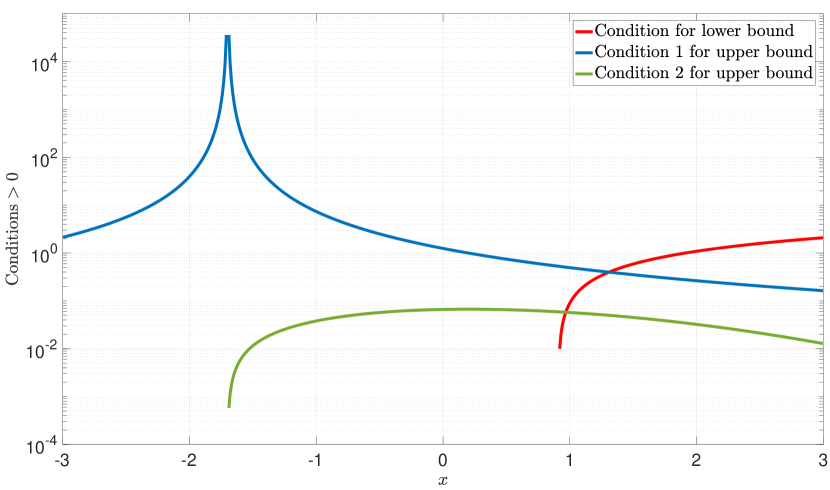
Figure 1: The conditions.

In Fig. 1, I illustrate the necessary conditions for Corollary 2 and Theorem 5 to hold jointly, when $b$ is not optimized. Specifically, in Fig. 1, the green and blue lines are the negative values of conditions (19) and (20), which are the necessary conditions for the upper bound in Corollary 2 to hold. Whereas, the red line is condition (44), which is the main necessary condition for the lower bound in Theorem 5 to hold. As this figure shows, it is necessary for $x$ to approximately be larger than one in order for both the lower and upper bounds to hold. As a result, the tail bounds are depicted for $x>1$ in Fig. 2.

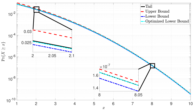
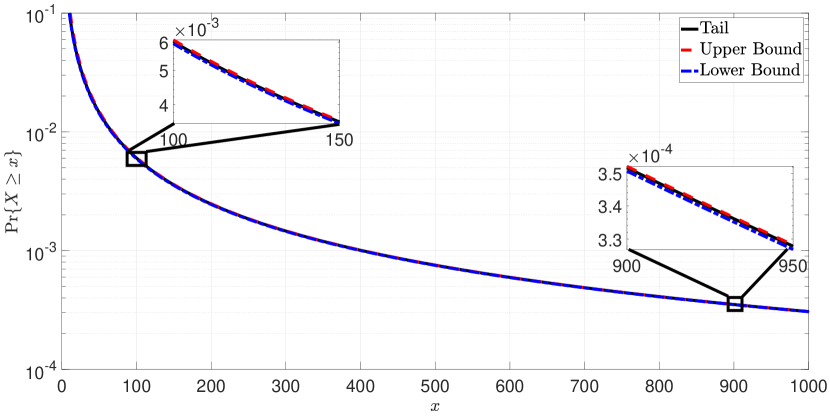
In Fig. 2, I show the tail probability, the upper bound from Corollary 2, the lower bound from Theorem 5 for $b=1$, and the lower bound from Theorem 5 for optimized $b=1$. As can be seen from the figure, the tail, the upper bound, and the lower bounds are almost indistinguishable. Due to this, I have provided two zoomed regions, from where the bounds are more visible. As $x$ increases, the bounds become even tighter, which can be see from the second zoomed region. The optimized lower bound is almost indistinguishable even in the first zoomed region, and almost identical to the tail bound in the second zoomed region.

Refer to caption
Figure 2: The tail, the bounds, and the optimized lower bound for the Gaussia RV.

If the expressions for the PDF and its derivative are plugged into the corresponding upper and lower bound for fixed $b$, the following bounds in closed form are obtained

$\displaystyle\frac{\sigma(x-\mu)^{b-1}}{\sqrt{2\pi}\left((x-\mu)^{b}+1\right)}e^{-\frac{(x-\mu)^{2}}{2\sigma^{2}}}\leq{\rm Pr}\{X\geq x\}\leq\frac{\sigma}{\sqrt{2\pi}(x-\mu)}e^{-\frac{(x-\mu)^{2}}{2\sigma^{2}}},$ (61)

which holds for $x>\mu$. A good choice for $b$ is $b=1$. Of course, the bounds in (61) hold when the corresponding conditions in Corollary 2 and Theorem 5 jointly hold.

As can be seen from (61), the bounds obtained with this method are one of the tightest bounds for the Gaussian tail available in the literature, see [12] for example. With this in mind, the tightness of the bounds illustrated in Fig. 2 is not surprising.

VII-B Non-Central and Central Chi-Square

The non-central and central chi-squared RVs have been one of those RVs whose tails have been hard to bound. This is one of the reasons why these RVs have been selected for numerical evaluation in this section. But it turns out that these two RVs are also very interesting from the perspective of the proposed bounds, as will be discussed in the following.

Since the non-central and central chi-squared RVs have support on $(0,\infty)$, Theorem 1 is applicable for the upper bound. Checking further if the optimal $a$ is $a\to\infty$, by checking if the conditions in Corollary 2 hold, reveals that the bound in Corollary 2 holds for $k\geq 2$, but it does not hold for $k=1$. Instead, for $k=1$, the conditions in Theorem 1 hold. Therefore, the cases for $k=1$ and $k\geq 2$ have to be separated.

VII-B1 The Case of $k\geq 2$

Since for $k\geq 2$, Corollary 2 holds for the upper bound I adopt Corollary 4 for the lower bound. Checking if the conditions in Corollary 4 are met for $b=1$, it is revealed that they indeed are met. Hence, since I am seeking simplicity of the bounds, I adopt $b=1$.

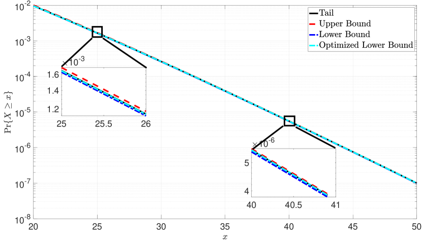
In Fig. 3, I plot the tail, the upper bound from Corollary 2, the lower bound from Corollary 4 for $b=1$ and for optimized $b$, for the case of the non-central chi-squared RV with parameters $k=6$ and $\lambda=0.2k$. Again, as can be seen from Fig. 3, the bounds are very tight.

Refer to caption
Figure 3: The tail, the bounds, and the optimized lower bound for the non-central chi-squared RV.

If the expressions for the PDF and its derivative of the non-central chi-squared RV are plugged into the corresponding upper and lower bound for fixed $b$, the following bounds in closed form are obtained

$\displaystyle-\frac{x^{b}}{1+x^{b}}\frac{\sqrt{\lambda x}\left(\frac{x}{\lambda}\right)^{k/4}I_{\frac{k-2}{2}}\left(\sqrt{x\lambda}\right){}^{2}}{(k-x-2)I_{\frac{k-2}{2}}\left(\sqrt{x\lambda}\right)+\sqrt{\lambda x}I_{\frac{k}{2}}\left(\sqrt{x\lambda}\right)}e^{-\frac{\lambda}{2}-\frac{x}{2}}$
$\displaystyle\leq{\rm Pr}\{X\geq x\}$
$\displaystyle\leq-\frac{\sqrt{\lambda x}\left(\frac{x}{\lambda}\right)^{k/4}I_{\frac{k-2}{2}}\left(\sqrt{x\lambda}\right){}^{2}}{(k-x-2)I_{\frac{k-2}{2}}\left(\sqrt{x\lambda}\right)+\sqrt{\lambda x}I_{\frac{k}{2}}\left(\sqrt{x\lambda}\right)}e^{-\frac{\lambda}{2}-\frac{x}{2}},$ (62)

which hold only when $k\geq 2$ and when $x$ in the denominator in (VII-B1) is large enough such that the denominator becomes negative, i.e., when

$\displaystyle(k-x-2)I_{\frac{k-2}{2}}\left(\sqrt{x\lambda}\right)+\sqrt{\lambda x}I_{\frac{k}{2}}\left(\sqrt{x\lambda}\right)<0.$ (63)

A good choice for $b$ in (VII-B1) is $b=1$.

Similar tightness of the bounds as in Fig. 3 are observed for the central chi-squared RV, for $k\geq 2$. Therefore, I omit this figure and only provide the analytical bounds. Specifically, if the expressions for the PDF and its derivative of the central chi-squared RV are plugged into the corresponding upper and lower bound for fixed $b$, the following bounds in closed form are obtained

$\displaystyle-\frac{2^{1-\frac{k}{2}}x^{b+\frac{k}{2}}}{\left(x^{b}+1\right)(k-x-2)\Gamma\left(\frac{k}{2}\right)}e^{-x/2}\leq{\rm Pr}\{X\geq x\}\leq-\frac{2^{1-\frac{k}{2}}x^{k/2}}{(k-x-2)\Gamma\left(\frac{k}{2}\right)}e^{-x/2},$ (64)

which hold only when $k\geq 2$ and when $x>k-2$. A good choice for $b$ in (64) is $b=1$.

VII-B2 The Case of $k=1$

The chi-squared distributions are defined for unit variance Gaussians. However, to generalize the result for $k=1$, I use the general form of the Gaussian squared distribution, given by

$\displaystyle f_{X}(x)=\frac{1}{2}\frac{1}{\sqrt{x}}\frac{1}{\sqrt{2\pi\sigma^{2}}}e^{-\frac{\left(\sqrt{x}+\mu\right)^{2}}{2\sigma^{2}}}+\frac{1}{2}\frac{1}{\sqrt{x}}\frac{1}{\sqrt{2\pi\sigma^{2}}}e^{-\frac{\left(\sqrt{x}-\mu\right)^{2}}{2\sigma^{2}}}.$ (65)

In this case, Theorem 1 is applicable for the upper bound. Since I am seeking for simplicity, I set $a=1$ in Theorem 1. I now have to look for the appropriate lower bound. One possibility is the bound in Theorem 3, for $a=1$. However, if the conditions in Theorem 3 are checked, one would obtain that they hold for very small $b$, in which case the convergence rate between the upper and lower bounds would be very slow. Another possibility is the lower bound in Corollary 4. Checking the conditions in Corollary 4, it turns out that they hold for $b=1$. Since I am seeking for simplicity of the bounds, the bound from Corollary 4 is adopted for $b=1$.

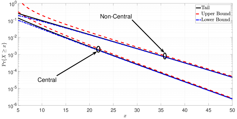
In Fig. 4, I plot the tail, the upper bound from Theorem 1 for $a=1$, the lower bound from Corollary 4 for $b=1$, for the Gaussian squared RV with $\sigma=1.5$ and $\mu=0$ (central), and for $\mu=-1.2$ (non-central). As can be seen, from Fig. 4, the bounds are tight and becoming tighter as $x$ grows. The bounds using optimized $a$ and $b$ are not shown as not to overcrowd the figure.

Refer to caption
Figure 4: The tail and the bounds for the Gaussian squared RV.

If the expressions for the PDF and its derivative of the Gaussian squared RV are plugged into the corresponding upper and lower bound for fixed $a=1$ and $b=1$, the following bounds in closed form are obtained

$\displaystyle\frac{\sigma x^{3/2}e^{-\frac{\left(\mu+\sqrt{x}\right)^{2}}{2\sigma^{2}}}\left(e^{\frac{2\mu\sqrt{x}}{\sigma^{2}}}+1\right)^{2}}{\sqrt{2\pi}(x+1)\left(x\left(e^{\frac{2\mu\sqrt{x}}{\sigma^{2}}}+1\right)+\sigma^{2}\left(e^{\frac{2\mu\sqrt{x}}{\sigma^{2}}}+1\right)-\mu\sqrt{x}\left(e^{\frac{2\mu\sqrt{x}}{\sigma^{2}}}-1\right)\right)}$
$\displaystyle\leq{\rm Pr}\{X\geq x\}$
$\displaystyle\leq\frac{\sigma\sqrt{x}e^{-\frac{\left(\mu+\sqrt{x}\right)^{2}}{2\sigma^{2}}}\left(e^{\frac{2\mu\sqrt{x}}{\sigma^{2}}}+1\right)^{2}}{\sqrt{2\pi}\left(x\left(e^{\frac{2\mu\sqrt{x}}{\sigma^{2}}}+1\right)-\sigma^{2}\left(e^{\frac{2\mu\sqrt{x}}{\sigma^{2}}}+1\right)-\mu\sqrt{x}\left(e^{\frac{2\mu\sqrt{x}}{\sigma^{2}}}-1\right)\right)},$ (66)

which holds when

$\displaystyle x\left(e^{\frac{2\mu\sqrt{x}}{\sigma^{2}}}+1\right)-\sigma^{2}\left(e^{\frac{2\mu\sqrt{x}}{\sigma^{2}}}+1\right)-\mu\sqrt{x}\left(e^{\frac{2\mu\sqrt{x}}{\sigma^{2}}}-1\right)>0,$ (67)

and is satisfied for large enough $x$.

VII-C Beta-Prime

The beta-prime RV is chosen since its PDF does not contain the exponential function.

Since the beta-prime RV has support on $[0,\infty)$, Theorem 1 is applicable for the upper bound. Checking further if the optimal $a$ is $a\to\infty$, by checking if the conditions in Corollary 2 hold, reveals that the bound in Corollary 2 does not hold. However, if the conditions in Corollary 1 are checked, then it is seen that the bound in Corollary 1 holds. Therefore, for simplicity, I adopt the bound from Corollary 1. Now for the lower bound, checking whether the conditions in Corollary 3 hold for $b=1$, it turns out that they not hold. One needs to set $b$ to e.g. $b=4/5$ in order for the conditions in Corollary 3, and the corresponding lower bound, to hold, for the chosen parameters. Another possibility is the lower bound in Corollary 4. Checking the conditions in Corollary 4, it turns out that they hold even for $b\to\infty$, but even then the convergence rate between the lower and upper bounds is poorer than for the case when the lower bound from Corollary 3 is chosen for $b=4/5$. Therefore, I pick $b=0.8$ in Corollary 3 as the lower bound.

In Fig. 5, I plot the tail, the upper bound from Corollary 1, the lower bound from Corollary 3 for $b=4/5$ for the beta-prime RV with parameters $\alpha=2.1$ and $\beta=1.3$. As can be seen, from Fig. 4, the bounds are again very tight.

Refer to caption
Figure 5: The tail and the bounds for the beta-prime RV.

If the expressions for the PDF and its derivative of the beta-prime RV are plugged into the corresponding upper and lower bound for $b=4/5$, the following bounds in closed form are obtained

$\displaystyle\frac{x^{\frac{4}{5}}}{1+x^{\frac{4}{5}}}\frac{x^{\alpha}(x+1)^{-\alpha-\beta+1}}{B(\alpha,\beta)(\beta x-\alpha)}\leq{\rm Pr}\{X\geq x\}\leq\frac{x^{\alpha}(x+1)^{-\alpha-\beta+1}}{B(\alpha,\beta)(\beta x-\alpha)},$ (68)

which holds when $x>\alpha/\beta$.

-D Proof Of Theorem 1

First note, that proving an upper bound for the right-tail ${\rm Pr}\{X\geq x\}=1-F_{X}(x)$ is equivalent to proving a lower bound for $F_{X}(x)$. Specifically, if $F_{X}(x)\geq P_{B}(x)$ holds, then the right-tail, ${\rm Pr}\{X\geq x\}$, is upper bounded as ${\rm Pr}\{X\geq x\}=1-F_{X}(x)\leq 1-P_{B}(x)$, where $P_{B}(x)$ is some function of $x$. In the following, I prove a lower bound for $F_{X}(x)$.

The integration by parts formula is given by

$\displaystyle\int\limits_{0}^{x}u(t)v^{\prime}(t)dt=v(t)u(t)\Bigg{|}_{0}^{x}-\int\limits_{0}^{x}v(t)u^{\prime}(t)dt.$ (69)

On the other hand, $F_{X}(x)$ is given by222Note that expanding (70) using Taylor series for some $x$, or expanding $f(t)$ for some $t$ and then integrating, does not lead to tight bounds.

$\displaystyle F_{X}(x)=\int_{0}^{x}f_{X}(t)dt.$ (70)

Applying the integration by parts on the integral in (70), where $u(t)=f_{X}(t)$ and $v^{\prime}(t)=dt$, and thereby $u^{\prime}(t)=f^{\prime}_{X}(t)$ and $v(t)=t$, leads to

$\displaystyle F_{X}(x)=tf_{X}(t)\Bigg{|}_{0}^{x}-\int\limits_{0}^{x}tf_{X}^{\prime}(t)dt$ (71)

or equivalently to

$\displaystyle F_{X}(x)=xf_{X}(x)-\int\limits_{0}^{x}tf_{X}^{\prime}(t)dt,$ (72)

where $\lim\limits_{x\to 0}xf_{X}(x)=0$ is due to assumption 6). As a result of (72), the following holds

$\displaystyle\dfrac{F_{X}(x)}{xf_{X}(x)-\int\limits_{0}^{x}tf_{X}^{\prime}(t)dt}=1.$ (73)

Now, taking the derivative with respect to $x$ on both sides of (73), I obtain

$\displaystyle\dfrac{d}{dx}\left[\dfrac{F_{X}(x)}{xf_{X}(x)-\int\limits_{0}^{x}tf_{X}^{\prime}(t)(t)dt}\right]=0.$ (74)

On the other hand, the derivative in (74) is obtained as

$\displaystyle\dfrac{d}{dx}\left[\dfrac{F_{X}(x)}{xf_{X}(x)-\int\limits_{0}^{x}tf_{X}^{\prime}(t)dt}\right]=\frac{F^{\prime}_{X}(x)}{H_{X}(x)}-\dfrac{F_{X}(x)}{H_{X}^{2}(x)}{H^{\prime}_{X}(x)},$ (75)

where

$\displaystyle F^{\prime}_{X}(x)$ $\displaystyle=f_{X}(x),$ (76)
$\displaystyle H_{X}(x)$ $\displaystyle=xf_{X}(x)-G_{X}(x),$ (77)
$\displaystyle G_{X}(x)$ $\displaystyle=\int\limits_{0}^{x}tf_{X}^{\prime}(t)dt,$ (78)
$\displaystyle H^{\prime}_{X}(x)$ $\displaystyle=f_{X}(x)+xf^{\prime}_{X}(x)-G^{\prime}_{X}(x).$ (79)

Note from (78) that

$\displaystyle G^{\prime}_{X}(x)=xf^{\prime}_{X}(x),$ (80)

however, I keep $G^{\prime}_{X}(x)$ as a separate auxiliary function.

Inserting (76), (77), and (79) into (75), and then inserting (75) into (74), I obtain

$\displaystyle\frac{f_{X}(x)}{xf_{X}(x)-G_{X}(x)}-\frac{F_{X}(x)}{(xf_{X}(x)-G_{X}(x))^{2}}\big{(}f_{X}(x)+xf^{\prime}_{X}(x)-G^{\prime}_{X}(x)\big{)}=0.$ (81)

From (81), I can obtain $F_{X}(x)$ as

$\displaystyle F_{X}(x)=\frac{xf_{X}^{2}(x)}{f_{X}(x)+xf^{\prime}_{X}(x)-G^{\prime}_{X}(x)}-\frac{f_{X}(x)G_{X}(x)}{f_{X}(x)+xf^{\prime}_{X}(x)-G^{\prime}_{X}(x)}.$ (82)

Note that if I insert (80) and (78) into (82) and simplify, I will obtain (72), which confirms the correctness of (82).

I now insert (80) into (82) but only into the second expression after the equality, and thereby obtain

$\displaystyle F_{X}(x)$ $\displaystyle=\frac{xf_{X}^{2}(x)}{f_{X}(x)+xf^{\prime}_{X}(x)-G^{\prime}_{X}(x)}-\frac{f_{X}(x)G_{X}(x)}{f_{X}(x)+xf^{\prime}_{X}(x)-xf^{\prime}_{X}(x)}$
$\displaystyle=\frac{xf_{X}^{2}(x)}{f_{X}(x)+xf^{\prime}_{X}(x)-G^{\prime}_{X}(x)}-\frac{f_{X}(x)G_{X}(x)}{f_{X}(x)},$ (83)

which leads to the final expression of $F_{X}(x)$ given by

$\displaystyle F_{X}(x)=\frac{xf_{X}^{2}(x)}{f_{X}(x)+xf^{\prime}_{X}(x)-G^{\prime}_{X}(x)}-G_{X}(x).$ (84)

I now make my main claim in this proof, which is that, under certain assumptions that will be specified later on, the following holds

$\displaystyle\frac{xf_{X}^{2}(x)}{f_{X}(x)+xf^{\prime}_{X}(x)-G^{\prime}_{X}(x)}-G_{X}(x)\geq\frac{x^{a}f_{X}^{2}(x)}{f_{X}(x)+x^{a}f^{\prime}_{X}(x)}+1,$ (85)

when (9) is met, where $a>0$.

Note that due to (84), the claim that (85) holds is equivalent to claiming that the following holds under certain conditions

$\displaystyle F_{X}(x)\geq\frac{x^{a}f_{X}^{2}(x)}{f_{X}(x)+x^{a}f^{\prime}_{X}(x)}+1.$ (86)

Now, since the claim that (85) holds, conditioned on (9) being satisfied, is equivalent to the claim that (86) holds, when (9) is met, I prove (86), which in fact is the main result of this theorem that I aim to prove.

I prove (86), under certain conditions that will be specified at the end, by proving that the function

$\displaystyle D_{X}(x)=F_{X}(x)-\frac{x^{a}f_{X}^{2}(x)}{f_{X}(x)+x^{a}f^{\prime}_{X}(x)}-1$ (87)

is $i)$ a decreasing function, and $ii)$ that it converges to zero as $x\to\infty$. The only possibility for $D_{X}(x)$ to be a decreasing function of $x$ and to $D_{X}(x)\to 0$ as $x\to\infty$ is for $D_{X}(x)$ to be positive function of $x$ that converges to zero as $x\to\infty$.

To prove $i)$, I need to prove that, under the later specified conditions, the following holds

$\displaystyle\dfrac{dD_{X}(x)}{dx}\leq 0.$ (88)

I now prove $i)$. The derivative of $D_{X}(x)$ with respect to $x$ is given by

$\displaystyle\dfrac{dD_{X}(x)}{dx}$ $\displaystyle=\frac{f_{X}(x)}{x\big{(}f_{X}(x)+x^{a}f^{\prime}_{X}(x)\big{)}^{2}}$
$\displaystyle\times\Big{(}(x-ax^{a})f^{2}_{X}(x)-x^{2a+1}\big{(}f^{\prime}_{X}(x)\big{)}^{2}+x^{a+1}f_{X}(x)\big{(}f^{\prime}_{X}(x)+x^{a}f^{\prime\prime}_{X}(x)\big{)}\Big{)}\leq 0.$ (89)

Note that the term

$\displaystyle\frac{f_{X}(x)}{x\big{(}f_{X}(x)+x^{a}f^{\prime}_{X}(x)\big{)}^{2}}$ (90)

in (-D) is positive. Hence, (88) holds if and only if

$\displaystyle(x-ax^{a})f^{2}_{X}(x)-x^{2a+1}\big{(}f^{\prime}_{X}(x)\big{)}^{2}+x^{a+1}f_{X}(x)\big{(}f^{\prime}_{X}(x)+x^{a}f^{\prime\prime}_{X}(x)\big{)}\leq 0.$ (91)

Hence, the necessary condition for $D_{X}(x)$ to be a decreasing function of $x$, i.e., (88) to hold, is (91) to hold. This concludes the proof of part $i)$.

To prove $ii)$, I need to prove that, under conditions (9) and (91), the following holds

$\displaystyle\lim_{x\to\infty}D_{X}(x)=0.$ (92)

Taking the limit of $D_{X}(x)$, I obtain

$\displaystyle\lim_{x\to\infty}D_{X}(x)$ $\displaystyle=\lim_{x\to\infty}\left(F_{X}(x)-\frac{x^{a}f_{X}^{2}(x)}{f_{X}(x)+x^{a}f^{\prime}_{X}(x)}-1\right)$ (93)
$\displaystyle=\lim_{x\to\infty}\big{(}F_{X}(x)-1\big{)}-\lim_{x\to\infty}\frac{x^{a}f_{X}^{2}(x)}{f_{X}(x)+x^{a}f^{\prime}_{X}(x)}$ (94)
$\displaystyle=-\lim_{x\to\infty}\frac{x^{a}f_{X}^{2}(x)}{f_{X}(x)+x^{a}f^{\prime}_{X}(x)}$ (95)
$\displaystyle=-\lim_{x\to\infty}\frac{x^{a}f_{X}^{2}(x)}{x^{a}f^{\prime}_{X}(x)}$ (96)
$\displaystyle=-\lim_{x\to\infty}\frac{f_{X}^{2}(x)}{f^{\prime}_{X}(x)}$ (97)
$\displaystyle=0.$ (98)

where (93) is obtained by inserting (87), (96) holds due to condition (9) and (5), and (98) holds due to assumption 5). Note that I have not invoked condition (91) for proving this limit. This concludes the proof of part $ii)$ part, and thereby concludes the proof of this theorem.

-E Proof Of Theorem 2

Let us define an auxiliary RV $Y$ as $Y=X-x_{0}$. Then the RV $Y$ has support on $([0,\infty)$ and as a result Theorem 1 holds. Consequently, the following holds

$\displaystyle{\rm Pr}\{Y\geq y\}\leq-\frac{y^{a}f_{Y}^{2}(y)}{f_{Y}(x)+y^{a}f^{\prime}_{Y}(y)}$ (99)

under conditions

$\displaystyle f_{Y}(y)+y^{a}f^{\prime}_{Y}(y)<0$ (100)
$\displaystyle(y-ay^{a})f^{2}_{Y}(y)-y^{2a+1}\big{(}f^{\prime}_{Y}(y)\big{)}^{2}+y^{a+1}f_{Y}(y)\big{(}f^{\prime}_{Y}(y)+y^{a}f^{\prime\prime}_{Y}(y)\big{)}\leq 0.$ (101)

On the other hand,

$\displaystyle{\rm Pr}\{X\geq x\}={\rm Pr}\{Y+x_{0}\geq x\}={\rm Pr}\{Y\geq x-x_{0}\}.$ (102)

As a result of (102) and (99), the following holds

$\displaystyle{\rm Pr}\{X\geq x\}={\rm Pr}\{Y\geq x-x_{0}\}\leq-\frac{(x-x_{0})^{a}f_{Y}^{2}(x-x_{0})}{f_{Y}(x-x_{0})+(x-x_{0})^{a}f^{\prime}_{Y}(x-x_{0})}$ (103)

under conditions

$\displaystyle f_{Y}(x-x_{0})+(x-x_{o})^{a}f^{\prime}_{Y}(x-x_{0})<0,$ (104)
$\displaystyle(x-x_{0}-a(x-x_{0})^{a})f^{2}_{Y}(x-x_{0})-(x-x_{0})^{2a+1}\big{(}f^{\prime}_{Y}(x-x_{0})\big{)}^{2}$
$\displaystyle+(x-x_{0})^{a+1}f_{Y}(x-x_{0})\big{(}f^{\prime}_{Y}(x-x_{0})+(x-x_{0})^{a}f^{\prime\prime}_{Y}(x-x_{0})\big{)}\leq 0.$ (105)

Now, since

$\displaystyle{\rm Pr}\{X\leq x\}={\rm Pr}\{Y+a\leq x\}={\rm Pr}\{Y\leq x-a\}.$ (106)

the following holds

$\displaystyle f_{X}(x)=f_{Y}(x-a).$ (107)

Furthermore, due to (107), the following holds

$\displaystyle f^{\prime}_{X}(x)=f^{\prime}_{Y}(x-a)$ (108)

and

$\displaystyle f^{\prime\prime}_{X}(x)=f^{\prime\prime}_{Y}(x-a).$ (109)

Inserting (107), (108), and (109) into (103), (104), and (105), I obtain that

$\displaystyle{\rm Pr}\{X\geq x\}\leq-\frac{(x-x_{0})^{a}f_{X}^{2}(x)}{f_{X}(x)+(x-x_{0})^{a}f^{\prime}_{X}(x)}$ (110)

under conditions

$\displaystyle f_{X}(x)+(x-x_{o})^{a}f^{\prime}_{X}(x)<0,$ (111)
$\displaystyle(x-x_{0}-a(x-x_{0})^{a})f^{2}_{X}(x)-(x-x_{0})^{2a+1}\big{(}f^{\prime}_{X}(x)\big{)}^{2}$
$\displaystyle+(x-x_{0})^{a+1}f_{X}(x)\big{(}f^{\prime}_{X}(x)+(x-x_{0})^{a}f^{\prime\prime}_{X}(x)\big{)}\leq 0,$ (112)

which is the result I aimed to prove.

-F Proof of Theorem 3

The same method is followed as in the proof of Theorem 1, with the following difference. I now need to prove an upper bound for $F_{X}(x)$ in order to obtain a lower bound for the right-tail ${\rm Pr}\{X\geq x\}=1-F_{X}(x)$.

I prove an upper bound for $F_{X}(x)$, and thereby prove (21), under certain conditions that will be specified at the end, by proving that the function

$\displaystyle D_{X}(x)=F_{X}(x)-\frac{x^{b}}{1+x^{b}}\frac{x^{a}f_{X}^{2}(x)}{f_{X}(x)+x^{b}f^{\prime}_{X}(x)}-1$ (113)

is $i)$ an increasing function and $ii)$ that it converges to zero as $x\to\infty$. The only possibility for $D_{X}(x)$ to be an increasing function of $x$ and to $D_{X}(x)\to 0$ as $x\to\infty$ is for $D_{X}(x)$ to be negative function of $x$ that converges to zero as $x\to\infty$.

To prove $i)$, I need to prove that, under the later specified conditions, the following holds

$\displaystyle\dfrac{dD_{X}(x)}{dx}\geq 0.$ (114)

The derivative of $D_{X}(x)$ with respect to $x$ is given by

$\displaystyle\dfrac{dD_{X}(x)}{dx}$ $\displaystyle=\dfrac{f_{X}(x)}{x\big{(}1+x^{b}\big{)}^{2}\big{(}f_{X}(x)+x^{a}f^{\prime}_{X}(x)\big{)}^{2}}$
$\displaystyle\times\Big{(}x\big{(}1+x^{b}\big{)}^{2}-x^{a+b}(a+b+ax^{b})f^{2}_{X}(x)-x^{2a+1}(x^{2b}-1)\big{(}f^{\prime}_{X}(x)\big{)}^{2}$
$\displaystyle+x^{a}f_{X}(x)\Big{[}x(1+x^{b})(2+x^{b})f^{\prime}_{X}(x)+x^{a+b}\big{(}-bf^{\prime}_{X}(x)+x(1+x^{b})f^{\prime\prime}_{X}(x)\big{)}\Big{]}\Big{)}\geq 0.$ (115)

Note that the term

$\displaystyle\dfrac{f_{X}(x)}{x\big{(}1+x^{b}\big{)}^{2}\big{(}f_{X}(x)+x^{a}f^{\prime}_{X}(x)\big{)}^{2}}$ (116)

in (-F) is positive. Hence, (114) holds if and only if

$\displaystyle x\big{(}1+x^{b}\big{)}^{2}-x^{a+b}(a+b+ax^{b})f^{2}_{X}(x)-x^{2a+1}(x^{2b}-1)\big{(}f^{\prime}_{X}(x)\big{)}^{2}$
$\displaystyle+x^{a}f_{X}(x)\Big{[}x(1+x^{b})(2+x^{b})f^{\prime}_{X}(x)+x^{a+b}\big{(}-bf^{\prime}_{X}(x)+x(1+x^{b})f^{\prime\prime}_{X}(x)\big{)}\Big{]}\geq 0$ (117)

holds.

To prove $ii)$, I need to prove that, under the later specified conditions, the following holds

$\displaystyle\lim_{x\to\infty}D_{X}(x)=0,$ (118)

which straightforward, given the proof of Theorem 1, after noting that

$\displaystyle\lim_{x\to\infty}\frac{x^{b}}{1+x^{b}}=1.$ (119)

for $b>0$. This concludes the proof of this theorem.

-G Proof of Theorem 5

I follow the same approach as for the proof of Theorem 3. Thereby,

$\displaystyle D_{X}(x)=F_{X}(x)-\frac{(x-\mu)^{b}}{1+(x-\mu)^{b}}\frac{f_{X}^{2}(x)}{f^{\prime}_{X}(x)}-1,$ (120)

and

$\displaystyle\dfrac{dD_{X}(x)}{dx}=\frac{f_{X}(x)}{\big{(}1+(x-\mu)^{b}\big{)}^{2}}$
$\displaystyle\times\Bigg{(}1-(x-\mu)^{2b}+\frac{f_{X}(x)}{\big{(}f^{\prime}_{X}(x)\big{)}^{2}}(x-\mu)^{b-1}\Big{(}-bf^{\prime}_{X}(x)+\big{(}1+(x-\mu)^{b}\big{)}(x-\mu)f^{\prime\prime}_{X}(x)\Bigg{)}.$ (121)

Noting that

$\displaystyle\frac{f_{X}(x)}{\big{(}1+(x-\mu)^{b}\big{)}^{2}}>0$ (122)

for $x>\mu$, it follows that

$\displaystyle\dfrac{dD_{X}(x)}{dx}\geq 0$ (123)

if an only if the following holds

$\displaystyle 1-(x-\mu)^{2b}+\frac{f_{X}(x)}{\big{(}f^{\prime}_{X}(x)\big{)}^{2}}(x-\mu)^{b-1}\Big{(}-bf^{\prime}_{X}(x)+\big{(}1+(x-\mu)^{b}\big{)}(x-\mu)f^{\prime\prime}_{X}(x)\geq 0.$ (124)

Given the proof of Theorem 3, the rest of the proof is straightforward and is therefore omitted.

References

  • [1] A. A. Markov, Ischislenie Veroiatnostei, 3rd ed.   Gosizdat, Moscow, 1913.
  • [2] I.-J. Bienaymé, Considérations à l’appui de la découverte de Laplace sur la loi de probabilité dans la méthode des moindres carrés.   Imprimerie de Mallet-Bachelier, 1853.
  • [3] P. L. Chebyshev, “Des valeurs moyennes,” Liouville’s J. Math. Pures Appl., vol. 12, pp. 177–184, 1867.
  • [4] H. Chernoff, “A measure of asymptotic efficiency for tests of a hypothesis based on the sum of observations,” The Annals of Mathematical Statistics, vol. 23, no. 4, pp. 493–507, 1952.
  • [5] W. Hoeffding, “Probability inequalities for sums of bounded random variables,” Journal of the American Statistical Association, vol. 58, no. 301, pp. 13–30, 1963.
  • [6] C. McDiarmid, On the method of bounded differences, ser. London Mathematical Society Lecture Note Series.   Cambridge University Press, 1989, p. 148–188.
  • [7] R. Ahlswede, P. Gács, and J. Körner, “Bounds on conditional probabilities with applications in multi-user communication,” Zeitschrift für Wahrscheinlichkeitstheorie und verwandte Gebiete, vol. 34, no. 2, pp. 157–177, 1976.
  • [8] T. M. Cover and J. A. Thomas, Elements of Information Theory (Wiley Series in Telecommunications and Signal Processing).   Wiley-Interscience, 2006.
  • [9] M. Ledoux, “On Talagrand’s deviation inequalities for product measures,” ESAIM: Probability and Statistics, vol. 1, p. 63–87, 1997.
  • [10] M. Talagrand, “Concentration of measure and isoperimetric inequalities in product spaces,” Publications Mathématiques de l’Institut des Hautes Etudes Scientifiques, vol. 81, pp. 73–205, 1995.
  • [11] S. Boucheron, G. Lugosi, and P. Massart, Concentration Inequalities: A Nonasymptotic Theory of Independence.   Oxford University Press, 2013.
  • [12] P. Borjesson and C.-E. Sundberg, “Simple approximations of the error function q(x) for communications applications,” IEEE Transactions on Communications, vol. 27, no. 3, pp. 639–643, 1979.