Reinforcement Learning for the Near-Optimal Design of Zero-Delay Codes for
Markov Sources

Abstract

In the classical lossy source coding problem, one encodes long blocks of source symbols that enables the distortion to approach the ultimate Shannon limit. Such a block-coding approach introduces large delays, which is undesirable in many delay-sensitive applications. We consider the zero-delay case, where the goal is to encode and decode a finite-alphabet Markov source without any delay. It has been shown that this problem lends itself to stochastic control techniques, which lead to existence, structural, and general structural approximation results. However, these techniques so far have only resulted in computationally prohibitive algorithmic implementations for code design. To address this problem, we present a practically implementable reinforcement learning design algorithm and rigorously prove its asymptotic optimality. In particular, we show that a quantized Q-learning algorithm can be used to obtain a near-optimal coding policy for this problem. The proof builds on recent results on quantized Q-learning for weakly Feller controlled Markov chains whose application necessitates the development of supporting technical results on regularity and stability properties, and relating the optimal solutions for discounted and average cost infinite horizon criteria problems. These theoretical results are supported by simulations.

I Introduction

I-A Zero-Delay Lossy Coding

We consider the problem of encoding an information source without delay, sending the encoded source over a discrete noiseless channel, and reconstructing the source, also without delay, at the decoder. Hence, the classical block-coding approach is not allowed.

The source $\{X_{t}\}_{t\geq 0}$ is a time-homogeneous, discrete-time Markov process taking values in a finite set $\mathbb{X}$ and has transition matrix $P(x_{t+1}|x_{t})$. We assume that the source is irreducible and aperiodic, and thus admits a unique invariant measure, which we will denote by $\zeta$. We also assume that the distribution of $X_{0}$, which we denote by $\pi_{0}$ (this can be different from $\zeta$), is available at the encoder and decoder. We will use the notation $\{X_{t}\}_{t\geq 0}\sim(\pi_{0},P)$ to indicate that the Markov process has initial distribution $\pi_{0}$ and transition matrix $P$.

At time $t\geq 0$, the encoded (compressed) information, denoted by $q_{t}$, is sent over a discrete noiseless channel with common input and output alphabet $\mathcal{M}\coloneqq\{1,\ldots,M\}$. The encoder is defined by an encoder policy $\gamma^{e}=\{\gamma^{e}_{t}\}_{t\geq 0}$, where $\gamma^{e}_{t}:\mathcal{M}^{t}\times\mathbb{X}^{t+1}\to\mathcal{M}$, and $q_{t}=\gamma^{e}_{t}(q_{[0,t-1]},X_{[0,t]})$, where we use the notation $X_{[0,t-1]}=(X_{0},\ldots,X_{t-1})$ and similarly for $q_{[0,t-1]}$. Note that for fixed $q_{[0,t-1]}$ and $X_{[0,t-1]}$, the map $\gamma^{e}_{t}(q_{[0,t-1]},X_{[0,t-1]},\,\cdot\,)$ is a quantizer (i.e. a map from $\mathbb{X}$ to $\mathcal{M}$), which we denote by $Q_{t}$. We will denote the set of all quantizers by $\mathcal{Q}$. Thus we can view an encoder policy at time $t$ as selecting a quantizer $Q_{t}\in\mathcal{Q}$ and then encoding (quantizing) $X_{t}$ as $q_{t}=Q_{t}(X_{t})$. We call such encoder policies admissible, and denote the set of all admissible encoder policies (sometimes called quantization policies) by $\Gamma^{e}$.

Upon receiving $q_{t}$, the decoder generates the reconstruction $\hat{X}_{t}$ without delay, using decoder policy $\gamma^{d}=\{\gamma^{d}_{t}\}_{t\geq 0}$, where $\gamma^{d}_{t}:\mathcal{M}^{t+1}\to\hat{\mathbb{X}}$ and where $\hat{\mathbb{X}}$ is a finite reproduction alphabet. Thus we have $\hat{X}_{t}=\gamma^{d}_{t}(q_{[0,t]})$. The set of these admissible decoder policies is denoted by $\Gamma^{d}$.

In general for the zero-delay coding problem, the goal is to minimize the average distortion (cost), given by

$$J(\pi_{0},\gamma^{e},\gamma^{d})\coloneqq\limsup_{T\to\infty}\mathbf{E}_{\pi_{0}}^{\gamma^{e},\gamma^{d}}\left[\frac{1}{T}\sum_{t=0}^{T-1}d(X_{t},\hat{X}_{t})\right],$$ (1)

where $d:\mathbb{X}\times\hat{\mathbb{X}}\to[0,\infty)$ is a given distortion measure and $\mathbf{E}_{\pi_{0}}^{\gamma^{e},\gamma^{d}}$ is the expectation with initial distribution $X_{0}\sim\pi_{0}$ under encoder policy $\gamma^{e}$ and decoder policy $\gamma^{d}$.

Since the source alphabet is finite, there clearly exists an optimal decoding policy for every encoding policy. Thus we identify a coding policy with the corresponding encoder policy by assuming that an optimal decoding policy is used for any given encoding policy and will denote $\gamma\coloneqq\gamma^{e}$ and $\Gamma\coloneqq\Gamma^{e}$. We can then restrict our search to finding optimal encoding policies. With an abuse of notation, we denote

$$J(\pi_{0},\gamma)\coloneqq\inf_{\gamma^{d}\in\Gamma^{d}}J(\pi_{0},\gamma^{e},\gamma^{d}).$$

The objective is then to minimize $J(\pi_{0},\gamma)$ over all $\Gamma$. We will denote the optimal cost by

$$J^{*}(\pi_{0})\coloneqq\inf_{\gamma\in\Gamma}J(\pi_{0},\gamma).$$

We will also consider the discounted cost problem, which is the minimization of

$$J_{\beta}(\pi_{0},\gamma^{e},\gamma^{d})\coloneqq\lim_{T\to\infty}\mathbf{E}_{\pi_{0}}^{\gamma^{e},\gamma^{d}}\left[\sum_{t=0}^{T-1}\beta^{t}d(X_{t},\hat{X}_{t})\right].$$ (2)

for some $\beta\in(0,1)$. As above, we assume an optimal decoder policy and minimize only over the encoder policies, yielding $J_{\beta}(\pi_{0},\gamma)$ and $J_{\beta}^{*}(\pi_{0})\coloneqq\inf_{\gamma\in\Gamma}J(\pi_{0},\gamma)$. We note that, as opposed to the optimal average distortion $J^{*}(\pi_{0})$, the quantity $J_{\beta}^{*}(\pi_{0})$ has little importance from a source coding point of view and we only use it as a tool toward designing codes that are near-optimal in the average distortion sense.

I-B Literature Review

A number of important structural results have been obtained for the preceding setup, starting with the foundational papers by Witsenhausen [1] and Walrand and Varaiya [2]. In particular, for the finite horizon problem, [1] showed that any encoder policy can be replaced, without performance loss, by one using only $q_{[0,t-1]}$ and $X_{t}$ to generate $q_{t}$. Furthermore, [2] proved a similar result for an encoder policy using only the conditional probability $P(X_{t}\in\,\cdot\,|q_{[0,t-1]})$ and $X_{t}$ to generate $q_{t}$. These results were generalized in further work, see e.g. [3, 4, 5, 6, 7]. In particular, [7] showed the existence of optimal policies in the infinite-horizon case, which we now review.

Let $\mathcal{P}(\mathbb{X})$ be the space of probability measures on $\mathbb{X}$ (where we endow this space with the weak convergence topology), and define the conditional probability $\pi_{t}\in\mathcal{P}(\mathbb{X})$ as the “belief” on $X_{t}$ given $q_{0},\ldots,q_{t-1}$, i.e.

$$\pi_{t}(A)\coloneqq P(X_{t}\in A|q_{[0,t-1]})$$ (3)

for all measurable $A\subset\mathbb{X}$.

Definition 1

We say an encoder policy $\gamma=\{\gamma_{t}\}_{t\geq 0}$ is of the Walrand-Varaiya type if, at time $t$, the policy uses only $\pi_{t}$ and $X_{t}$ to generate $q_{t}$. That is, $\gamma$ selects a quantizer $Q_{t}=\gamma_{t}(\pi_{t})$ and $q_{t}$ is generated as $q_{t}=Q_{t}(X_{t})$. Such a policy is called stationary if it does not depend on $t$. We denote the set of stationary Walrand-Varaiya type policies by $\Gamma_{\text{WS}}$.

Remark: We note that $\pi_{t}$ can be obtained from $\pi_{t-1}$ and $q_{t-1}$ (see the update equation (4)). Since the initial distribution $\pi_{0}$ is know to both the encoder and decoder, the decoder can track $\pi_{t}$ and $Q_{t}$ for all $t\geq 0$.

Proposition 1

[7, Theorem 3] There exists an optimal policy $\gamma^{*}\in\Gamma_{\text{WS}}$ for the average cost problem (1). That is, there exists $\gamma^{*}\in\Gamma_{\text{WS}}$ such that

$$J(\pi_{0},\gamma^{*})=J^{*}(\pi_{0})\text{\ \ for all $\pi_{0}$}.$$

Proposition 2

[7, Proposition 2] For any $\beta\in(0,1)$, there exists an optimal policy $\gamma_{\beta}^{*}\in\Gamma_{\text{WS}}$ for the discounted cost problem (2). That is, there exists $\gamma^{*}\in\Gamma_{\text{WS}}$ such that

$$J_{\beta}(\pi_{0},\gamma^{*})=J_{\beta}^{*}(\pi_{0})\text{\ \ for all $\pi_{0}$}.$$

Despite the key structural results obtained for this problem reviewed above, finding an optimal policy for either finite or infinite horizons is difficult. For some very special cases, such solutions do exist. For example, [2] showed memoryless encoding is optimal when $\mathbb{X}=\mathcal{M}$ and the channel is noisy and symmetric. However, for a general source and channel (or for a noiseless channel, as in this paper), finding an optimal encoding policy is an open problem.

Stochastic control based approaches play an important role in the above structural results. Under a stochastic control framework, [1, 2] used dynamic programming, [7, 11, 12] made use of the value iteration algorithm and the vanishing discount method, whereas [6] used the convex analytic method to obtain structural results for optimal codes. A key component in these results is that the zero-delay coding problem can be restated as a Markov Decision Process (MDP), with $\{\pi_{t}\}_{t\geq 0}$ as the state process. However, there are limitations when using these methods to obtain an optimal solution. In particular, dynamic programming relies on backwards induction from a finite time horizon, which is not applicable for the infinite horizon case. Furthermore, the implementation of the value iteration algorithm requires the computation of certain value functions and conditional expectations, which is practically very challenging due to the probability measure-valued state dynamics.

These challenges, which will be made more explicit in Section III-A, motivate the use of a reinforcement learning approach that we present in this paper. A popular reinforcement learning algorithm, Q-learning [13, 14, 15, 16, 10, 17] is primarily used for fully observed finite space MDPs. This algorithm does not require the knowledge of the transition kernel, or even the cost (or reward) function, for its implementation. In this algorithm, the incurred per-stage cost variable is observed through the simulation of a single sample path. When the state and action spaces are finite, under mild conditions that require that all state-action pairs are visited infinitely often, this algorithm is known to converge to the optimal cost. Recently, this algorithm has been generalized to be applicable for continuous space MDPs (see [18] and the references therein).

In the broader literature related to zero-delay coding, often information theoretic relaxation techniques are used to convexify the non-convex zero-delay optimal quantization problem, which lead to lower bounds on optimal performance, as well as to upper bounds. These include replacing the number of bins constraint with a mutual information constraint, applying the Shannon lower bounding technique, or entropy coding (see, e.g., [19], [20] [21]). Using ergodicity and invariance properties, [22] has constructed time-invariant coding schemes using dithering. A further line of work for linear systems follow the sequential rate-distortion theoretic approach [23, 24, 25, 21, 26, 27]. For coding of Gaussian sources over additive Gaussian channels, some of these results become operational for zero-delay coding [23]; see also [25],[28], and [29].

We note that applying learning theoretic methods in the theory of optimal (lossy) source coding has prior history. A well established line of study of this problem focuses on empirical learning methods for data compression [30, 31, 32], though often limited to i.i.d source models. Our approach here is complementary, since we consider a highly structured coding problem instead of (unstructured) vector quantization and we consider sources with memory. Our analysis leads to near-optimal solutions directly (without learning the source distribution). We also refer recent research activity in machine learning methods in communications theory (see e.g. [33]); however, our analysis seems to be the first contribution to source coding in the context of reinforcement learning.

Contributions.

We formulate the zero-delay coding problem so that it is amenable to a reinforcement learning approach. In particular, the MDP associated with our zero-delay lossy coding problem has an uncountable state space (the set of beliefs) and thus has to be discretized (quantized) to apply Q-learning. After posing the problem as a weak Feller MDP, we build on recent results from [18] to rigorously justify the convergence of a reinforcement learning algorithm to a near-optimal solution (depending on the discretization on the state space), first for the discounted cost problem, and then for the average cost problem. In particular, [18] showed that, under mild assumptions, a Q-learning algorithm in which the state is quantized converges to the optimal solution as the maximum diameter of the quantization bins for the state space goes to zero. However, the results of [18] cannot be straightforwardly applied to our zero-delay coding problem and there are several additional ingredients needed for our analysis: (a) The convergence and near-optimality was shown in [18] only for the discounted cost criterion problem. Our focus is the average cost setup; this will be addressed via relating discounted cost optimal coding policies to ones that are near-optimal for the average cost. (b) We also need to prove several technical results that are necessary for applying the algorithm in [18], such as the unique ergodicity under an exploration policy which has not been studied for our setup. Specifically, our main contributions are the following:

• We present a reinforcement learning algorithm for the near-optimal design of stationary zero-delay codes (Algorithm 1). As an auxiliary result, we state the near-optimality of the algorithm for the discounted cost problem when the source starts from the invariant distribution (Theorem 1). Then we show that an optimal policy for the discounted cost problem (for sufficiently large discount parameter) can be used to obtain a near-optimal policy for the average cost problem (Theorem 2). This gives, to our knowledge, the first concrete implementation of a provably near-optimal algorithm for the zero-delay coding problem.

• To show convergence of the algorithm, we prove additional regularity properties of the MDP formulation of the zero-delay coding problem. In particular, we show that the process $\{\pi_{t}\}_{t\geq 0}$ is stable under a memoryless exploration policy, and then deduce unique invariance under this same policy, which is necessary for the application of [18].

• Finally, Section VI provides simulations comparing Algorithm 1 with the so called omniscent finite-state scalar quantization (O-FSSQ) design algorithm [34, Chapter 14], a heuristic, but effective technique for designing zero-delay lossy codes, to demonstrate the superior performance of Algorithm 1.

The rest of the paper is organized as follows: In Section II we present our reinforcement learning algorithm and in Theorem 1 and Theorem 2 state the near-optimality of the resulting stationary policies for the discounted and average cost problems, respectively, when the source starts from its invariant distribution. In Section III-A we review how the zero-delay coding problem can be turned into a problem involving an MDP. After describing our motivation to apply Q-learning to this problem, in Section III-C we present in detail the quantized Q-learning algorithm in [18]. In Section IV we prove the unique ergodicity of our MDP under a memoryless exploration policy and identify some key features of this unique invariant measure, which is needed to prove our main results. Section V contains the proofs of the main results and Section VI presents simulation results. Conclusions are drawn in Section VII, where future research directions are also discussed. Some technical results relating discounted cost optimal and average cost optimal policies are relegated to the Appendix.

II Near-Optimal Design of Zero-Delay Codes

In order to make the algorithm self-contained, we first introduce some definitions and update equations. The rationale for these will be formalized during the proof of convergence to near-optimality.

Recall the definition of the belief $\pi_{t}$ in (3). Under a Walrand-Varaiya type policy, $\pi_{t+1}$ can be obtained from $\pi_{t}$ and $Q_{t}$ via the update equation [6]

$$\pi_{t+1}(x_{t+1})=\frac{1}{\pi_{t}(Q_{t}^{-1}(q_{t}))}\smashoperator[r]{\sum_{x_{t}\in Q_{t}^{-1}(q_{t})}^{}}P(x_{t+1}|x_{t})\pi_{t}(x_{t}),$$ (4)

where $Q_{t}^{-1}(q_{t})=\{x\in\mathbb{X}:Q_{t}(x)=q_{t}\}$.

Recall that $\mathcal{Q}$ is the set of all quantizers from $\mathbb{X}\to\mathcal{M}$. Then we define $c:\mathcal{P}(\mathbb{X})\times\mathcal{Q}\to\mathbb{R}_{+}$ as

$$c(\pi,Q)\coloneqq\sum_{i=1}^{M}\min_{\hat{x}\in\hat{\mathbb{X}}}\sum_{x\in Q^{-1}(i)}\pi(x)d(x,\hat{x}).$$ (5)

Let $m\coloneqq\left|\mathbb{X}\right|$. Given a fixed parameter $n\in\mathbb{Z}_{+}$, we define

$$\mathcal{P}_{n}(\mathbb{X})\coloneqq\left\{\hat{\pi}\in\mathcal{P}(\mathbb{X}):\hat{\pi}=\left(\frac{k_{1}}{n},\ldots,\frac{k_{m}}{n}\right),k_{i}\in\mathbb{Z}_{+},\,i=1,\ldots,m\right\}.$$ (6)

Given any $\pi\in\mathcal{P}(\mathbb{X})$, let $\hat{\pi}$ denote the nearest neighbour of $\pi$ (in Euclidean distance) in $\mathcal{P}_{n}(\mathbb{X})$. We note that $\hat{\pi}$ can be effectively calculated using [35, Algorithm 1], which we include as Algorithm 2 in the Appendix for convenience. This algorithm “quantizes” $\pi\in\mathcal{P}(\mathbb{X})$ to its nearest neighbor in $\mathcal{P}_{n}(\mathbb{X})$.

For technical reasons, we impose the following assumption on the invariant distribution $\zeta$.

Assumption 1

The measure $\zeta\in\mathcal{P}(\mathbb{X})$ is in the interior of some quantization bin of the nearest neighbor mapping implemented by Algorithm 2.

Remark: Note that this assumption is met by almost every source $\{X_{t}\}_{t\geq 0}$ in the sense that if the transition matrix $P$ is chosen randomly according to the uniform distribution over $\mathcal{P}(\mathbb{X})$, then the probability that the corresponding invariant measure $\zeta$ lies on a decision boundary is zero.

Finally, consider a $\mathcal{P}(\mathbb{X})\times\mathcal{Q}$-valued sequence $\{\pi_{t},Q_{t}\}_{t\geq 0}$ and the resulting $\mathcal{P}_{n}(\mathbb{X})\times\mathcal{Q}$-valued sequence $\{\hat{\pi}_{t},Q_{t}\}_{t\geq 0}$, where $\hat{\pi}_{t}$ is the nearest neighbor of $\pi_{t}$ in $\mathcal{P}_{n}(\mathbb{X})$. Then we define $\mathsf{Q}_{t}$ and $\alpha_{t}$, which are both functions from $\mathcal{P}_{n}(\mathbb{X})\times\mathcal{Q}$ to $[0,\infty)$, by

$$\mathsf{Q}_{0}(\hat{\pi},Q) \equiv 0$$

$$\mathsf{Q}_{t+1}(\hat{\pi}_{t},Q_{t}) =(1-\alpha_{t}(\hat{\pi}_{t},Q_{t}))\mathsf{Q}_{t}(\hat{\pi}_{t},Q_{t})+\alpha_{t}(\hat{\pi}_{t},Q_{t})[c(\pi_{t},Q_{t})+\beta\;\underset{v\in\mathcal{Q}}{\text{min}}\;\mathsf{Q}_{t}(\hat{\pi}_{t+1},v)]$$ (7)

$$\mathsf{Q}_{t+1}(\hat{\pi},Q) =\mathsf{Q}_{t}(\hat{\pi},Q)\quad\text{for all }(\hat{\pi},Q)\neq(\hat{\pi}_{t},Q_{t})$$

$$\alpha_{t}(\hat{\pi},Q) =\frac{1}{1+\sum_{k=0}^{t}1_{(\hat{\pi}_{k},Q_{k})=(\hat{\pi},Q)}}$$ (8)

Algorithm 1: Q-learning for Near-Optimal Zero-Delay Quantization

1:source alphabet $\mathbb{X}$, channel alphabet $\mathcal{M}$, transition kernel $P(x_{t+1}|x_{t})$, invariant distribution $\zeta$, quantization parameter $n$, discount factor $\beta\in(0,1)$

2:Sample $X_{0}$ according to $\zeta$

3:Quantize $\pi_{0}$ using Algorithm 2 with parameter $n$ to obtain $\hat{\pi}_{0}$

4:Randomly select quantizer $Q_{0}$ uniformly from $\mathcal{Q}$

5:$q_{0}=Q_{0}(x_{0})$

6:for $t\geq 0$ do

7:  Compute $c(\pi_{t},Q_{t})$ using (5)

8:  Generate $x_{t+1}$ according to $P(x_{t+1}|x_{t})$

9:  Compute $\pi_{t+1}$ using (4)

10:  Quantize $\pi_{t+1}$ using Algorithm 2 with parameter $n$ to obtain $\hat{\pi}_{t+1}$

11:  Update $\mathsf{Q}_{t+1}$ and $\alpha_{t+1}$ using (7) and (8)

12:  Randomly select quantizer $Q_{t+1}$ uniformly from $\mathcal{Q}$

13:  $q_{t+1}=Q_{t+1}(x_{t+1})$

14:end for

The following is one of our main results, which shows convergence of this algorithm to a near-optimal policy for the discounted cost (distortion) problem if $\pi_{0}=\zeta$, the unique invariant initial distribution. Note that in this case $\{X_{t}\}_{t\geq 0}$ is a stationary and ergodic source. The proof of this result is given in Section V.

Theorem 1 (Discounted distortion)

Let Assumption 1 hold. Then for any $n\geq 1$ and $\beta\in(0,1)$, the sequence $\{\mathsf{Q}_{t}\}_{t\geq 0}$ converges almost surely to a limit $\mathsf{Q}^{*}$. For any $\pi\in\mathcal{P}(\mathbb{X})$, let $\hat{\pi}$ denote the nearest neighbor of $\pi$ in $\mathcal{P}_{n}(\mathbb{X})$ and define the encoding policy $\gamma_{\beta,n}(\pi)$ by setting

$$\gamma_{\beta,n}(\pi)=\operatorname*{argmin}_{Q\in\mathcal{Q}}\mathsf{Q}^{*}(\hat{\pi},Q).$$ (9)

Then, for any $\epsilon>0$ and $\beta\in(0,1)$, there exists $N\geq 1$ such that

$$J_{\beta}(\zeta,\gamma_{\beta,n})\leq J^{*}_{\beta}(\zeta)+\epsilon$$

for all $n\geq N$.

Remarks:

• We note that $\mathsf{Q}^{*}(\pi,Q)$ is the expected value of the discounted cost obtained by a policy that takes “action” $Q$ (i.e., uses the quantizer $Q$) at an initial state $\pi$, and then follows the optimal policy for the rest of the time. Due to the step where the minimum of $\mathsf{Q}^{*}(\hat{\pi},Q)$ is considered instead of that of $\mathsf{Q}^{*}(\pi,Q)$, the encoding policy $\gamma_{\beta,n}(\pi)$ is a piecewise constant function of the actual belief $\pi\in\mathcal{P}(\mathbb{X})$.

• In the theorem we have used the limiting Q-value $\mathsf{Q}^{*}$ to derive the desired policy $\gamma_{\beta,n}$. Similar (probabilistic and in-expectation) bounds can be given if we use $\mathsf{Q}_{t}$ for some large $t$, at the expense of a more involved analysis.

In the preceding theorem the discounted cost (distortion) is considered, a quantity which has limited significance in source coding. The next theorem, which is the main result of this paper, shows that the policy obtained in Theorem 1, for $\beta$ close enough to $1$ and $n$ large enough is also a near-optimal policy for the average cost (distortion) problem. The result is proved in Section V.

Theorem 2 (Average distortion)

Let Assumption 1 hold and let $\epsilon>0$ be arbitrary. Then for all sufficiently large $\beta\in(0,1)$, there exists $N(\beta)\geq 1$ such that

$$J(\zeta,\gamma_{\beta,n})\leq J^{*}(\zeta)+\epsilon$$

for all $n\geq N(\beta)$, where $\gamma_{\beta,n}$ is the policy obtained in (9) of Theorem 1.

III Quantized Q-learning for Near-Optimal Zero-Delay Quantization

III-A Zero-Delay Coding as a Markov Decision Process (MDP)

Recall the update equation (3). This shows that $\pi_{t+1}$ is conditionally independent of $(\pi_{[0,t-1]},Q_{[0,t-1]})$ given $\pi_{t}$ and $Q_{t}$, and hence $\{\pi_{t}\}_{t\geq 0}$ is an MDP with control $\{Q_{t}\}_{t\geq 0}$.

To make the MDP well-defined with regard to its regularity properties (such as continuity), we place the following topology on quantizers. Let $Q\in\mathcal{Q}$, and call $B_{i}=Q^{-1}(i)$ the $i^{th}$ bin of $Q$, for $i\in\mathcal{M}$. Following [36, 6], $Q$ can be represented as a stochastic kernel from $\mathbb{X}$ to $\mathcal{M}$ such that $Q(i|x)=1_{\{x\in B_{i}\}},i\in\mathcal{M}$. Then for $P\in\mathcal{P}(\mathbb{X})$, we denote by $PQ$ the joint probability measure $PQ(x,i)=P(x)Q(i|x),(x,i)\in\mathbb{X}\times\mathcal{M}$.

Definition 2

[36] A sequence $\{Q_{n}\}_{n\geq 0}\subset\mathcal{Q}$ converges to $Q\in\mathcal{Q}$ weakly at input $P$ if $PQ_{n}\to PQ$ weakly.

Under this topology [6], we will denote the transition kernel induced by the update equation (4) by
$P(d\pi_{t+1}|\pi_{t},Q_{t})$. A key property of this transition kernel is the following:

Lemma 1

[6, Lemma 11]. For any $\gamma\in\Gamma_{\text{WS}}$, the transition kernel $P(d\pi_{t+1}|\pi_{t},Q_{t})$ is weakly continuous in $(\pi_{t},Q_{t})$. That is,

$$\int_{\mathcal{P}(\mathbb{X})}f(\pi^{\prime})P(d\pi^{\prime}|\pi,Q)$$

is continuous on $\mathcal{P}(\mathbb{X})\times\mathcal{Q}$ for all continuous bounded $f$.

Recall the cost function (5), and note that this is the average distortion if the optimal decoder is used for a given $Q_{t}$. Then, by our assumption that we are using an optimal decoder for a given encoder of the Walrand-Varaiya type, we have

$$\mathbf{E}_{\pi_{0}}^{\gamma}\bigl{[}c(\pi_{t},Q_{t})\bigr{]}=\mathbf{E}_{\pi_{0}}^{\gamma}\bigl{[}d(X_{t},\hat{X}_{t})\bigr{]},$$

for all $t\geq 0$. Thus, we may replace $d(X_{t},\hat{X}_{t})$ with $c(\pi_{t},Q_{t})$ in our minimization of the average and discounted cost. This allows us to formulate the zero-delay coding problem as an MDP with state space $\mathcal{P}(\mathbb{X})$, action space $\mathcal{Q}$, transition kernel $P(d\pi_{t+1}|\pi_{t},Q_{t})$, and cost function $c(\pi_{t},Q_{t})$.

III-B Motivation for Reinforcement Learning

The MDP formulation of the zero-delay coding problem has many analytical advantages. For example, it allows the use of dynamic programming and value iteration methods to prove existence results. However, this representation entails several limitations. In particular, even though our original source $\{X_{t}\}_{t\geq 0}$ takes finitely many values, admits a unique invariant measure, and has explicit transition probabilities given by $P(x_{t+1}|x_{t})$, the MDP representation has $\{\pi_{t}\}_{t\geq 0}$ as its state process, which takes values in the uncountable set $\mathcal{P}(\mathbb{X})$, and it has an analytically complicated transition probability $P(d\pi_{t+1}|\pi_{t},Q_{t})$ induced by the update equation (4). This makes actual implementation of dynamic programming and value iteration for the computation of optimal policies difficult.

In particular, a traditional approach to obtain an optimal policy for the discounted cost problem is to use the value iteration algorithm given by

$$J_{t}(\pi)=\min_{Q\in\mathcal{Q}}\Bigl{[}c(\pi,Q)+\beta\int_{\mathcal{P}(\mathbb{X})}J_{t-1}(\pi^{\prime})P(d\pi^{\prime}|\pi,Q)\Bigr{]},$$

for $t\in\{1,2,\ldots\}$, with $J_{0}(\pi)=0$. It can be shown that our MDP satisfies the necessary conditions for the convergence $J_{t}(\pi_{0})\to J^{*}_{\beta}(\pi_{0})$ as $t\to\infty$ to hold, and the actions obtaining the above minimum converge to an optimal policy [7].

It turns out however that actually computing this value function is difficult; the values clearly cannot be computed directly for each state as the state space is uncountable. An approach would be to quantize the MDP via an approximate model whose solution is near-optimal for the original model (e.g. via [37, Theorem 4.27]). For zero-delay quantization, such an approximate model would require numerical simulations for the computation of transition probabilities, as one would need to place a probability measure on sets of probability measures.

Thus, computing the above values is very difficult except in trivial cases. This motivates the use of a reinforcement learning algorithm in which the transition probabilities are not computed or estimated explicitly.

III-C Quantized Q-learning for Near-Optimal Zero-Delay Quantization

A common reinforcement learning algorithm for finding optimal policies is Q-learning, in which empirical value functions are recursively updated based on observed realizations of the state, action, and cost. Such an algorithm is guaranteed to converge to an optimal policy for the discounted cost problem, but only in situations where the state and action spaces are finite (among other mild assumptions, see [13]), and thus it is not applicable in our case.

A solution is “quantized” Q-learning, where we approximate the original MDP using an MDP with a finite state space, and run Q-learning on this model. Recent work [18] and [38] give conditions under which the resulting policy is near-optimal for the original MDP. We note that such a quantization strategy is not limited to a Q-learning approach. For example, [39] considers a quantized value iteration approach, but while this solves the issue of the uncountable state space, one must still contend with the difficult state dynamics given by $P(\,\cdot\,|\pi,Q)$. Furthermore, in such a quantization procedure, one must compute probability measures over the transition kernel itself, which makes the problem even more challenging. A Q-learning approach avoids all of this complexity by learning the values empirically.

First, we state the assumptions necessary to apply quantized Q-learning to a general MDP. In the proof of our main result, we will later show that these assumptions hold for the zero-delay coding MDP. Consider an MDP with $\mathsf{Z}$-valued state $\{Z_{t}\}_{t\geq 0}$ having initial condition $Z_{0}=z_{0}$, $\mathsf{U}$-valued control $\{U_{t}\}_{t\geq 0}$, transition kernel $P(\,\cdot\,|z,u)$ and cost function $c:\mathsf{Z}\times\mathsf{U}\to[0,\infty)$

Assumption 2

The MDP has the following properties:

1. The stochastic kernel $P(\cdot|z,u)$ is weakly continuous in $(z,u)$, i.e. $P(\cdot|z_{n},u_{n})\to P(\cdot|z,u)$ weakly for all $(z_{n},u_{n})\to(z,u)$.

2. The cost function $c$ is continuous and bounded.

3. The action space $\mathsf{U}$ is finite.

4. The state space $\mathsf{Z}$ is a compact subset of a Euclidean space.

Let $\{B_{i}\}_{i=1}^{N}$ be a partition of $\mathsf{Z}$ into compact subsets and let $\mathsf{Y}\coloneqq\{y_{1},\ldots,y_{N}\}$, where $y_{i}\in B_{i}$. We define a quantizer on $\mathsf{Z}$ as a mapping $f:\mathsf{Z}\to\mathsf{Y}$, such that

$$f(z)=y_{i}\quad\text{if}\;z\in B_{i}.$$

Note that when we first introduced quantizers in Section I, we were considering quantizers of the information source $\{X_{t}\}_{t\geq 0}$. Although the idea is the same here, we emphasize that we are now considering quantization of the state space of an MDP.

We also define the maximum radius of the $B_{i}$:

$$d_{\infty}\coloneqq\max_{i=1,\ldots,N}\max_{z\in B_{i}}\|z-y_{i}\|.$$

We now introduce the quantized Q-learning algorithm. Here, we let $y\in\mathsf{Y}$ and $Y_{t}\coloneqq f(Z_{t})$. Also, we apply a policy $\eta\coloneqq\{\eta_{t}\}_{t\geq 0}$, where $\eta_{t}:\mathsf{Y}^{t+1}\times\mathsf{U}^{t}\to\mathsf{U}$. Finally, we define the $\mathsf{Q}$-factors $\{\mathsf{Q}_{t}\}_{t\geq 0}$ and the learning rate $\{\alpha_{t}\}_{t\geq 0}$, where both $\mathsf{Q}_{t}$ and $\alpha_{t}$ are maps from $\mathsf{Y}\times\mathsf{U}$ to $[0,\infty)$.

Quantized Q-learning[18]

1:Set $Z_{0}=z_{0}$

2:for $t\geq 0$ do

3:  $U_{t}=\eta_{t}(Y_{[0,t]},U_{[0,t-1]})$

4:  Sample $Z_{t+1}\sim P(\,\cdot\,|Z_{t},U_{t})$

5:  if $(Y_{t},U_{t})=(y,u)$ then

6:   $\mathsf{Q}_{t+1}(y,u)=(1-\alpha_{t}(Y_{t},U_{t}))\mathsf{Q}_{t}(Y_{t},U_{t})+\alpha_{t}(Y_{t},U_{t})[c(Z_{t},U_{t})+\beta\;\underset{v\in\mathsf{U}}{\text{min}}\;\mathsf{Q}_{t}(Y_{t+1},v)]$

7:  else

8:   $\mathsf{Q}_{t+1}(y,u)=\mathsf{Q}_{t}(y,u)$

9:  end if

10:end for

Definition 3

We say a policy $\eta$ is a memoryless exploration policy if for all $t\geq 0$

$$\Pr(\eta_{t}(\,\cdot\,)=u_{i})=p_{i},\quad i=1,\ldots,|\mathsf{U}|,$$

where $p_{i}>0$ for all $i$ and $\sum_{i}p_{i}=1$, and we have enumerated the (finite) action space as $\mathsf{U}=\{u_{1},u_{2},\ldots,u_{|\mathsf{U}|}\}$. That is, the policy chooses actions independently and randomly.

Assumption 3

In the above algorithm, we have

1. $\alpha_{t}(y,u)=\frac{1}{1+\sum_{k=0}^{t}1_{(Y_{k},U_{k})=(y,u)}}$.

2. The policy $\eta$ used is a memoryless exploration policy.

3. Under $\eta$, the state process $\{Z_{t}\}_{t\geq 0}$ admits a unique invariant measure $\psi$.

Theorem 3

[18, Corollary 11] Under Assumptions 2 and 3, $\mathsf{Q}_{t+1}$ in the above algorithm converges to a limit $\mathsf{Q}^{*}$. Furthermore, consider the policy obtained through

$$\eta^{*}(z)=\operatorname*{argmin}_{v\in\mathsf{U}}\mathsf{Q}^{*}(f(z),v).$$

Then,

$$\big{|}J_{\beta}(z,\eta^{*})-J^{*}_{\beta}(z)\big{|}\to 0\text{ \ as \ $d_{\infty}\to 0$}.$$

for all $z\in\mathsf{Z}$ such that $Y_{t}=f(z)$ infinitely often almost surely. That is, the policy obtained by taking the minimizing actions of $\mathsf{Q}^{*}$ and then making it constant over the quantization bins is near-optimal for fine enough quantization, provided the bins are hit infinitely often.

Remark: The original result from [18] requires that every bin is hit infinitely often, and so the resulting policy is near-optimal over all of $\mathsf{Z}$. The slightly modified version here, where we only use bins that are hit infinitely often, holds from identical arguments.

Returning to our application, we want to apply this algorithm to the MDP defined in Section III-A. Using the notation of this section, we have $\mathsf{Z}=\mathcal{P}(\mathbb{X})$ and $\mathsf{U}=\mathcal{Q}$, with the cost function (5) and transition kernel $P(d\pi_{t+1}|\pi_{1},Q_{t})$. We let $\mathsf{Y}=\mathcal{P}_{n}(\mathbb{X})$ (recall (6)). We will show that Assumptions 2 and 3 hold for this setup. The most challenging of these will be verifying Assumption 3 (iii), so we begin with that proof.

IV Unique Ergodicity Under a Memoryless Exploration Policy

To show the desired result, we will need the following supporting results from the literature of partially observed Markov processes (POMPs). In this section, our MDP will be driven by a memoryless exploration policy given in Definition 3.

IV-A Predictor and Filter Merging

In this section, we call $\pi_{t}$ the predictor, and we also introduce the following probability measure on $\mathbb{X}$, often called the filter in the literature:

$$\overline{\pi}_{t}(A)\coloneqq P(X_{t}\in A|q_{[0,t]}).$$

The filter admits a recursion equation similar to (4) (see e.g. [40, 41, 42]). Note that these recursions are dependent on the initialization of $\pi_{0}$, also called the prior. We denote the predictor (respectively, filter) process resulting from the prior $\pi_{0}=\nu$ as $\{\pi_{t}^{\nu}\}_{t\geq 0}$ (respectively, $\{\overline{\pi}_{t}^{\nu}\}_{t\geq 0}$).

Definition 4

Let $\nu,\mu\in\mathcal{P}(\mathbb{X})$. The total variation distance is

$$\|\nu-\mu\|_{TV}\coloneqq\sup_{\|f\|_{\infty}\leq 1}\Bigl{|}\int f\,d\nu-\int f\,d\mu\Bigr{|},$$

where the supremum is taken over all measurable $f:\mathbb{X}\to[-1,1]$.

Definition 5

We say that the predictor (respectively, filter) process is stable in total variation in expectation if for any $\mu,\nu\in\mathcal{P}(\mathbb{X})$ such that $\mu$ is absolutely continuous with respect to $\nu$, we have

$$\lim_{n\to\infty}E^{\mu}[\|\pi_{t}^{\mu}-\pi_{t}^{\nu}\|_{TV}]=0.$$

We will use the following lemmas to deduce predictor stability.

Lemma 2

[41, Theorem 2.11] The filter is stable in total variation in expectation if and only if the predictor is stable in total variation in expectation.

Lemma 3

[42, Corollary 5.5] Let $\{X_{t}\}_{t\geq 0}$ be a discrete-time Markov chain and $\{Y_{t}\}_{t\geq 0}$ be a stochastic process such that the $Y_{t}$ are conditionally independent given $\{X_{t}\}_{t\geq 0}$ and $P(Y_{t}|X_{s\geq 0})$ has the form

$$P(Y_{t}\in A|X_{s\geq 0})=\int_{A}g(X_{t},y)\phi(dy),$$

where $g(x,y)$ is a probability density with respect to the $\sigma$-finite measure $\phi$. If $g$ is strictly positive, and $\{X_{t}\}_{t\geq 0}$ is positive Harris recurrent and aperiodic, then the filter $\overline{\pi}_{t}(A)\coloneqq P(X_{t}\in A|y_{[0,t]})$ is stable in total variation in expectation.

Lemma 4

Under any memoryless exploration policy, the filter process $\{\overline{\pi}_{t}\}_{t\geq 0}$ is stable in total variation in expectation.

Proof:

We have

$$P(q_{t}|x_{t}) =\sum_{Q_{t}}P(q_{t}|x_{t},Q_{t})P(Q_{t}|x_{t})$$

$$=\sum_{Q_{t}}1_{\{Q_{t}(x_{t})=q_{t}\}}P(Q_{t}|x_{t})=\smashoperator[lr]{\sum_{\{Q_{t}:Q_{t}(x_{t})=q_{t}\}}^{}}P(Q_{t}|x_{t}).$$

where the second equality follows from the fact that $q_{t}=Q_{t}(x_{t})$ is deterministic. Now, under a memoryless exploration policy, the quantizer $Q_{t}$ is chosen independently and randomly, so $P(Q_{t}|x_{t})=P(Q_{t})$. Thus we have

$$P(q_{t}|x_{t})=\smashoperator[lr]{\sum_{\{Q_{t}:Q_{t}(x_{t})=q_{t}\}}^{}}P(Q_{t}).$$

Since we are considering the set of all possible quantizers, for any $(x_{t},q_{t})\in\mathbb{X}\times\mathcal{M}$, the set $\{Q_{t}:Q_{t}(x_{t})=q_{t}\}$ is nonempty. Under a memoryless exploration policy, $P(Q_{t})>0$ for all $Q_{t}$. Thus $P(q_{t}|x_{t})>0$ everywhere. Then we use Lemma 3 to conclude that the filter is stable in total variation in expectation. ∎

Lemmas 2 and 3 immediately imply the following:

Corollary 1

Under any memoryless exploration policy, the predictor process $\{\pi_{t}\}_{t\geq 0}$ is stable in total variation in expectation.

Theorem 4

Under any memoryless exploration policy, the process $\{\pi_{t}\}_{t\geq 0}$ admits a unique invariant measure.

Proof:

The proof slightly generalizes an argument presented in [43, Corollary 3]. Throughout, we use the notation $\nu(f)\coloneqq\int fd\nu$. Note that, under any Walrand-Varaiya type policy (and in particular, under a memoryless exploration policy), the processes $\{\pi_{t}\}_{t\geq 0}$ and $\{(X_{t},\pi_{t})\}_{t\geq 0}$ are Markov. Let $T$ and $S$ be the transition operators associated with $\{\pi_{t}\}_{t\geq 0}$ and $\{(X_{t},\pi_{t})\}_{t\geq 0}$, respectively. Recall that $\zeta$ is the unique invariant measure of our source $\{X_{t}\}_{t\geq 0}$.

First note that since since the exporation policy is memoryless, the process $\{\pi_{t}\}_{t\geq 0}$ itself it weak Feller (not just the controlled process). Since every Markov process with a weakly continuous kernel on a compact state space admits an invariant measure (see, e.g., [44]), $\{\pi_{t}\}_{t\geq 0}$ has an invariant measure. Thus, we are left with proving uniqueness. Assume that $m_{1},m_{2}\in\mathcal{P}(\mathbb{X}\times\mathcal{P}(\mathbb{X}))$ are two invariant measures for $\{(X_{t},\pi_{t})\}_{t\geq 0}$. Then their projections on $\mathbb{X}$ are invariant for $\{X_{t}\}_{t\geq 0}$. Then, by unique invariance of $\zeta(dx)$ we have

$$m_{i}(dx,d\nu)=P_{m_{i}}(d\nu|x)\zeta(dx).$$

We now show that $m_{1}(F)=m_{2}(F)$ for each $F$ on a set of measure-determining functions, namely those such that $F(x,\nu)=\phi(x)H(\nu(\phi_{1}),\ldots,\nu(\phi_{l}))$, where $\phi\in C(\mathbb{X}),\phi_{1},\ldots,\phi_{l}\in C(\mathbb{X})$, $H$ is bounded and Lipschitz continuous with constant $L_{H}$, and $l\in\mathbb{Z}_{+}$ [43].

By invariance we have, for $i=1,2$, that

$$m_{i}(F)=\smashoperator[l]{\int_{\mathbb{X}\times\mathcal{P}(\mathbb{X})}^{}}\frac{1}{n}\sum_{j=0}^{n-1}S^{j}F(x,\nu)P_{m_{i}}(d\nu|x)\zeta(dx).$$

Thus,

$$|m_{1}(F)-m_{2}(F)|$$

$$\leq\int\limits_{\mathbb{X}\times\mathcal{P}(\mathbb{X})\times\mathcal{P}(\mathbb{X})}\frac{1}{n}\sum_{j=0}^{n-1}|S^{j}F(x,\nu_{1})-S^{j}F(x,\nu_{2})|$$

$$\hskip 110.00017pt\cdot P_{m_{1}}(d\nu_{1}|x)P_{m_{2}}(d\nu_{2}|x)\zeta(dx)$$

$$\leq L_{H}\|\phi\|\quad\quad\smashoperator[l]{\int_{\mathbb{X}\times\mathcal{P}(\mathbb{X})\times\mathcal{P}(\mathbb{X})}^{}}\frac{1}{n}\sum_{j=0}^{n-1}E^{\mu}[\sum_{i=1}^{l}|\pi_{j}^{\nu_{1}}(\phi_{i})-\pi_{j}^{\nu_{2}}(\phi_{i})|]$$

$$\hskip 110.00017pt\cdot P_{m_{1}}(d\nu_{1}|x)P_{m_{2}}(d\nu_{2}|x)\zeta(dx).$$

Since the predictors are stable in total variation in expectation, and by the dominated convergence theorem, the last integral converges to zero as $n\to\infty$. Then, the joint process $\{(X_{t},\pi_{t})\}_{t\geq 0}$ admits at most one invariant measure. Next we show that $\{\pi_{t}\}_{t\geq 0}$ admits at most one invariant measure.

Assume that $v_{1},v_{2}\in\mathcal{P}(\mathcal{P}(\mathbb{X}))$ are two different invariant measures for $\{\pi_{t}\}_{t\geq 0}$. Then there exists $f\in C(\mathcal{P}(\mathbb{X}))$ continuous such that $v_{1}(f)\neq v_{2}(f)$. Now for $j=1,2$, let $\{(X^{j}_{t},\pi^{j}_{t})\}_{t\geq 0}$ be the process with initial law $\pi(dx)v_{j}(d\pi)$. Since $\mathbb{X}$ is finite, $P(X_{t}^{j}\in\,\cdot\,,\pi_{t}^{j}\in\,\cdot\,)$ is tight.

Now, by Lemma 1 and since $\mathbb{X}$ is finite, we also have that $\{(X_{t},\pi_{t})\}_{t\geq 0}$ has a weakly continuous transition kernel. Thus the time average

$$\frac{1}{T}\sum_{t=0}^{T-1}P(X^{j}_{t}\in\,\cdot\,,\pi^{j}_{t}\in\,\cdot\,)$$

converges weakly to an invariant measure $\eta_{j}$ for $\{(X_{t},\pi_{t})\}_{t\geq 0}$ [45, Theorem 3.3.1].

Then for $F(x,\pi)=f(x)$, we have $\eta_{1}(F)=v_{1}(f)\neq v_{2}(f)=\eta_{2}(f)$. But then $\eta_{1}$ and $\eta_{2}$ are two different invariant measures for $\{(X_{t},\pi_{t})\}_{t\geq 0}$, which is a contradiction. Thus $\{\pi_{t}\}_{t\geq 0}$ admits at most one invariant measure.

∎

IV-B Properties of the Unique Invariant Measure

Recall from Theorem 3 that the resulting policy is only near-optimal over bins that are hit infinitely often; this section identifies some of these bins for the zero-delay coding MDP. Throughout, for any measure $\pi\in\mathcal{P}(\mathbb{X})$, we denote its nearest neighbor in $\mathcal{P}_{n}(\mathbb{X})$ by $\hat{\pi}$ (recall that this nearest neighbor map is performed using Algorithm 2).

Let $\eta$ be an arbitrary but fixed memoryless exploration policy, and let $\phi$ be the unique invariant measure for $\{\pi_{t}\}_{t\geq 0}$ under $\eta$, as in Theorem 4. Not every element of $\mathcal{P}_{n}(\mathbb{X})$ (recall (6)) is hit infinitely often under $\eta$. As a trivial example, take the case where $\{X_{t}\}_{t\geq 0}$ is independent and identically distributed (i.i.d.) with distribution given by $P$. Then we have $\pi_{t}(x)=P(x)$ for all $t\geq 1$, so that only $\hat{P}\in\mathcal{P}_{n}(\mathbb{X})$ is visited infinitely often.

To address this issue, consider the pushforward measure of $\phi$ induced by the nearest neighbor map from $\mathcal{P}(\mathbb{X})$ to $\mathcal{P}_{n}(\mathbb{X})$. That is, consider the measure $\hat{\phi}\in\mathcal{P}(\mathcal{P}_{n}(\mathbb{X}))$ defined by

$$\hat{\phi}(\hat{\pi})\coloneqq\phi\left(\{\pi\in\mathcal{P}(\mathbb{X}):f(\pi)=\hat{\pi}\}\right),$$

where we have used $f(\pi)=\hat{\pi}$ to denote the nearest neighbour mapping from $\mathcal{P}(\mathbb{X})$ to $\mathcal{P}_{n}(\mathbb{X})$. Then consider the following set,

$$\mathcal{P}_{n}^{\phi}(\mathbb{X})\coloneqq\left\{\hat{\pi}\in\mathcal{P}_{n}(\mathbb{X}):\hat{\phi}(\hat{\pi})>0\right\}.$$ (10)

Lemma 5

Let $\pi_{0}=\zeta$; that is, let $X_{0}$ be distributed according to the invariant probability measure. Then under a memoryless exploration policy $\eta$, for every $\hat{\pi}\in\mathcal{P}_{n}^{\phi}(\mathbb{X})$, we have $\hat{\pi}_{t}=\hat{\pi}$ infinitely often almost surely.

Proof:

Consider the predictor processes under $\eta$ and let $\pi_{0}=\zeta$. Using the notation from the previous section, we denote this process by $\{\pi^{\zeta}_{t}\}_{t\geq 0}$. By predictor stability (Corollary 1) and by the same steps as in the proof of Theorem 4, we have that for any measurable and bounded function $g:\mathcal{P}(\mathbb{X})\to\mathbb{R}$, as $N\to\infty$,

$$\int\zeta(dx_{0})\frac{1}{N}\sum_{t=0}^{N-1}g(\pi_{t}^{\zeta})\to\int g(\pi)\phi(d\pi)$$ (11)

almost surely. Now let $g$ be the indicator function of the quantization bin of the nearest neighbor map $f$ corresponding to some $\hat{\pi}\in\mathcal{P}_{n}^{\phi}(\mathbb{X})$; that is, $g(\pi)=1$ if $f(\pi)=\hat{\pi}$ and $g(\pi)=0$ otherwise. Then (11) implies that any bin which has positive measure under $\phi$ must be hit infinitely often almost surely by $\pi^{\zeta}_{t}$. But this is exactly how we defined $\mathcal{P}_{n}^{\phi}(\mathbb{X})$; it is the set of all $\hat{\pi}$ whose bins have positive measure under $\phi$. Therefore every $\hat{\pi}\in\mathcal{P}_{n}^{\phi}(\mathbb{X})$ is hit infinitely often almost surely. ∎

The following lemma and corollary ensure that the bin of $\zeta$ is hit infinitely often, and thus that the policy obtained through quantized Q-learning will be near-optimal when $\pi_{0}=\zeta$.

Lemma 6

We have $\zeta\in\text{supp}(\phi)$, where $\text{supp}(\phi)$ denotes the support of $\phi$ in $\mathcal{P}(\mathbb{X})$.

Proof:

Consider some neighborhood of radius $\delta$ containing $\zeta$, say $N_{\delta}(\zeta)\subset\mathcal{P}(\mathbb{X})$. Now consider a totally “uninformative” quantizer $\overline{Q}\in\mathcal{Q}$; that is $\overline{Q}(x)=i$ for all $x\in\mathbb{X}$ and some $i\in\mathcal{M}$. Via the update equation (4), if $Q_{t}=\overline{Q}$, we have that $\pi_{t+1}=\pi_{t}P$. By a classical result of Dobrushin [46], there exists some $T>0$ such that for all $\pi\in\mathcal{P}(\mathbb{X})$, $\pi P^{T}\in N_{\delta}(\zeta)$. Thus, if $Q_{t}=\overline{Q}$ for $t=0,\ldots,T-1$, then we have $\pi_{T}\in N_{\delta}(\zeta)$.

But $\eta$ is a memoryless exploration policy, so it has some fixed positive probability of choosing $\overline{Q}$, say $P(\eta(\pi)=\overline{Q})=p>0$. In particular, for all $t\geq T$, $P(\pi_{t}\in N_{\delta}(\zeta)|\pi_{0})\geq P(Q_{[t-T,t-1]}=\overline{Q})=p^{T}$. This implies that $\zeta$ is “accessible” (see [47, Definition 2.1]) and hence that $\zeta\in\text{supp}(\phi)$ [47, Lemma 2.2]. ∎

Note that Lemma 6 does not necessarily imply that $\hat{\zeta}\in\mathcal{P}_{n}^{\phi}(\mathbb{X})$, since is only guarantees that every neighborhood of $\zeta$ has positive measure. If $\zeta$ happens to be on a bin boundary, it may be that $\zeta$ is the only element in its bin that lives in the support and that $\hat{\zeta}$ is not hit infinitely often. This is why we introduced Assumption 1 in Section II.

Corollary 2

Under Assumption 1, $\hat{\zeta}\in\mathcal{P}_{n}^{\phi}(\mathbb{X})$.

Proof:

Since $\zeta$ is not on a bin boundary, simply take $\delta$ in the proof of Lemma 6 small enough so that all of $N_{\delta}(\zeta)$ is mapped to $\hat{\zeta}$. Then $\phi(N_{\delta}(\zeta))>0$ implies that $\hat{\phi}(\hat{\zeta})>0$, so $\hat{\zeta}\in\mathcal{P}_{n}^{\phi}(\mathbb{X})$. ∎

V Proofs of Main Results

We are now ready to show that Assumptions 2 and 3 hold for our quantized MDP with components

$$\mathsf{Z}=\mathcal{P}(\mathbb{X}),\;\mathsf{Y}=\mathcal{P}_{n}(\mathbb{X}),\;\mathsf{U}=\mathcal{Q},\;P=P(\,\cdot\,|\pi,Q),\;c=c(\pi,Q).$$ (12)

Recall that $f$ maps $\pi\in\mathcal{P}(\mathbb{X})$ to its nearest neighbor $\hat{\pi}\in\mathcal{P}_{n}(\mathbb{X})\subset\mathcal{P}(\mathbb{X})$.

Lemma 7

The above MDP satisfies Assumptions 2 and 3.

Proof:

We begin with Assumption 2: (i) holds by Lemma 1. (ii) is clear from our definition of $c$ in (5). Since $\mathbb{X}$ and $\mathcal{M}$ are finite, $\mathcal{Q}$ is finite, so (iii) holds. Finally, $\mathbb{X}$ is finite, so $\mathcal{P}(\mathbb{X})$ is compact, so (iv) holds.

We now show Assumption 3: (i) and (ii) hold in Algorithm 1 based on the update equation (8) and from the uniform selection of $Q_{t+1}\in\mathcal{Q}$. Finally, (iii) holds due to Theorem 4. ∎

We can now prove our main results.

Proof:

Algorithm 1 is simply the quantized Q-learning algorithm in Section III applied to the quantized zero-delay coding MDP in (12), and using a uniform exploration policy. Note that as $n\to\infty$,

$$\max_{\pi\in\mathcal{P}(\mathbb{X})}\min_{\hat{\pi}\in\mathcal{P}_{n}(\mathbb{X})}\|\pi-\hat{\pi}\|_{2}=O\Big{(}\frac{1}{n^{2}}\Big{)}\to 0,$$

so we have $d_{\infty}\to 0$ as $n\to\infty$. Note that by Theorem 3, the policy $\gamma_{\beta,n}$ is only near-optimal over bins that are hit infinitely often, which by Lemma 5 includes the set

$$\left\{\pi\in\mathcal{P}(\mathbb{X}):\hat{\pi}\in\mathcal{P}_{n}^{\phi}(\mathbb{X})\right\}.$$ (13)

But we have under Assumption 1 and Corollary 2 that $\zeta$ is indeed in this set. Then by Lemma 7 we can apply Theorem 3 when $\pi_{0}=\zeta$. Thus for any $\beta\in(0,1)$ and $\epsilon>0$ we can choose $N$ such that for all $n\geq N$ in Algorithm 1,

$$J_{\beta}(\zeta,\gamma_{\beta,n})\leq J^{*}_{\beta}(\zeta)+\epsilon$$ (14)

as claimed. ∎

Proof:

We will use Theorem 5 in the Appendix that, loosely speaking, states that if a policy is near-optimal for a discount factor $\beta$ close enough to $1$, then this policy is also near-optimal for the average cost. Let us verify that the conditions of the theorem are met when $\mathsf{Z}=\mathcal{P}(\mathbb{X})$, $\mathsf{U}=\mathcal{Q}$, $P(\,\cdot\,|z,u)=P(\,\cdot\,|\pi,Q)$, and $c(z,u)=c(\pi,Q)$. Indeed, (i)-(iii) are met by the definition of $c(\pi,Q)$ since $\mathcal{P}(\mathbb{X})$ is the standard probability simplex in $\mathbb{R}^{|\mathbb{X}|}$ and $\mathcal{Q}$ is finite. Condition (iv) is true by Lemma 1, and (v) is holds by [7, Lemma 1], which states that for any $\pi,\pi^{\prime}\in\mathcal{P}(\mathbb{X})$,

$$\left|J^{*}_{\beta}(\pi)-J^{*}_{\beta}(\pi^{\prime})\right|\leq K\rho_{1}(\pi,\pi^{\prime})\leq K|\mathbb{X}|,$$

where $K$ is some constant and $\rho_{1}$ is the $L_{1}$ Wasserstein distance on $\mathcal{P}(\mathbb{X})$ [48].

Now let $\epsilon>0$ and let $N(\beta)\geq 1$ be such that the policy $\gamma_{\beta,n}$ in Theorem 1 satisfies $J_{\beta}(\zeta,\gamma_{\beta,n})\leq J^{*}_{\beta}(\zeta)+\frac{\epsilon}{2(1-\beta)}$ for all $n\geq N(\beta)$. Then we can apply Theorem 5 with $\epsilon$ replaced by $\epsilon/2$ and $\delta$ replaced by $\frac{\epsilon}{2(1-\beta)}$ to conclude that for all $\beta\in(0,1)$ close enough to $1$, the average cost performance of $\gamma_{\beta,n}$ satisfies

$$J(\zeta,\gamma_{\beta,n})\leq J^{*}(\zeta)+\epsilon\text{\ \ for all $\pi_{0}\in\mathcal{P}(\mathbb{X})$}$$

for all $n\geq N(\beta)$, which completes the proof. ∎

Remark: Note that due to the way the discounted cost scales with $\beta$, the policy $\gamma_{\beta,n}$ in the proof does not have to be $\epsilon$-optimal for the discounted cost, but rather it can be chosen to be only $\frac{\epsilon}{2(1-\beta)}$-optimal.

VI Simulations

In the simulations we use mean-squared error (MSE) $d(x,\hat{x})=(x-\hat{x})^{2}$ as our distortion measure and when using Algorithm 1 we fix the discount factor at $\beta=0.9999$. We let $\pi_{0}=\zeta$, so that Theorem 2 is applicable. When testing algorithm performance, we take the average distortion over $10^{6}$ samples, which we denote by $D$, and calculate the signal-to-noise ratio (SNR) according to

$$\text{SNR}=10\log_{10}\left(\frac{\text{var}(X)}{D}\right),$$

where $\text{var}(X)$ is the variance of the stationary Markov source $\{X_{t}\}_{t\geq 0}$. We plot the SNR for varying quantizer rates, which is given by $R=\log_{2}(|\mathcal{M}|)$. Finally, in all of the simulations we take $\hat{\mathbb{X}}=\mathbb{X}\subset\mathbb{R}$.

On algorithm complexity and time to convergence

Note the set $\mathcal{P}_{n}(\mathbb{X})$, and thus the state space of our quantized MDP, has size $\left|\mathcal{P}_{n}(\mathbb{X})\right|=$ ${n+|\mathbb{X}|-1}\choose{|\mathbb{X}|-1}$ [35]. Furthermore, our action space, if we include every possible quantizer from $\mathbb{X}\to\mathcal{M}$, has size $\mathcal{Q}=|\mathcal{M}|^{|\mathbb{X}|}$. Although these both grow quickly in their respective parameters, we note that the actual utilized state and action spaces tend to be much smaller. Indeed, $\mathcal{P}_{n}^{\phi}(\mathbb{X})$ tends to be much smaller than $\mathcal{P}_{n}(\mathbb{X})$; as an extreme case, for an independent and identically distributed (i.i.d.) source, $\mathcal{P}_{n}^{\phi}(\mathbb{X})$ has only one element. Also, many quantizers do not need to be considered (for example, those with empty bins, and for certain distortion measures those with non-convex bins). Thus, the actual number of states and convergence time will generally be much less than the theoretical upper bound. Note that for linear learning rates (as in our algorithm), the required number of iterations for convergence is polynomial in $|\mathcal{P}_{n}(\mathbb{X})|\times|\mathcal{Q}|$ (see [49] for related bounds on convergence time for Q-learning).

VI-A Finite-Alphabet Markov Sources

For finite-state Markov sources, we compare Algorithm 1 against an omniscient finite-state scalar quantizer (O-FSSQ) [34, Chapter 14] as this method seems to be the most competitive among zero-delay code designs for Markov sources. In this algorithm, one fixes a quantizer $V$ from $\mathbb{X}$ to $\{1,\ldots,K\}$, where $\{1,\ldots,K\}$ is a finite set of “states”. A sequence of training data is sorted into subsequences based on the state of the preceding data point. A Lloyd-Max quantizer [50] is then designed for each of these subsequences. However, in implementation the decoder does not know exactly the state of the preceding data point, so it uses $V(\hat{X}_{t})$, rather than $V(X_{t})$, as the state. That is, if $V(\hat{X}_{t})=i\in\{1,\ldots,K\}$, then to quantize $X_{t+1}$ one uses the Lloyd-Max quantizer corresponding to the $i$th subsequence. The O-FSSQ is known to perform very well for many common Markov sources and on real-world sampled data.

The O-FSSQ employs a strategy similar to Algorithm 1 in the sense that it uses a finite set of “states” at time $t-1$ to select a quantizer at time $t$. While simple to implement and relatively fast to train, the O-FSSQ design is based on heuristic principles and has no guarantee for optimality or near-optimality, unlike our Algorithm 1. Note that since $\hat{\mathbb{X}}$ is finite, the O-FSSQ is limited to using at most $K=|\hat{\mathbb{X}|}$ states. On the other hand, in Algorithm 1 we can let the number of states be larger in order to obtain a better performance.

In the simulations we consider a stationary Markov source with common source and reproduction alphabet $\mathbb{X}=\hat{\mathbb{X}}=\{1,\ldots,8\}$. The transition matrix and the unique invariant distribution are given in the Appendix in (21) and (22), respectively. In Fig. 1 we plot SNR values for $|\mathcal{M}|=2,\ldots,6$, so the rates range from $R=1$ to $R=\log_{2}(6)$. We include an O-FSSQ designed with $K=8$ states, using $10^{6}$ training samples. We include two comparisons with Algorithm 1. The first is with $n=1$, which yields $8$ states. The second is with $n=5$, which gives ${12}\choose{7}$$=792$ possible states, but at most $30$ are actually utilized in the final design.

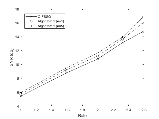
Figure 1: Comparison of Algorithm 1 with O-FSSQ for finite Markov source

Note that even when using the same number of states, Algorithm 1 outperforms the O-FSSQ. At rate $R=1$, the SNR gain over the O-FSSQ is 0.31 dB for $n=1$ and 0.53 dB for $n=5$. At rate $R=\log_{2}(6)=2.58$, the SNR gain over the O-FSSQ is 1.25 dB for $n=1$ and 2.09 dB for $n=5$.

Moreover, Algorithm 1 can be used with a larger number of states, giving performance gains. Of course, this comes at a cost of overall codebook size, as a different quantizer/codebook must be stored for each different state.

VI-B Continuous Markov Sources

While the mathematical analysis presented in the paper does not cover the continuous case, as future work we intend to develop a rigorous treatment of the continuous source setup. The weak Feller and ergodicity results follow as before, building on the analysis in [6] that used the convex analytic method to obtain structural results for continuous space Markov models; however the unbounded cost will require additional analysis. Nonetheless, in this section, we demonstrate that the algorithm is also suitable for continuous sources as quantization of the probability measures can be done in a variety of efficient ways, facilitating reinforcement learning.

Notably, [51] and [52, Section V.C] propose a scheme in which a probability measure is first approximated by one with finite support, then further quantized using Algorithm 2. Under certain assumptions, this was shown to be an efficient method for quantizing probability measures under a Wasserstein metric, and consequently, the weak convergence topology.

In particular for our algorithm, one computes $\hat{\pi}_{t}\in\mathcal{P}_{n}(\mathbb{X})$ by first approximating $\pi_{t}\in\mathcal{P}(\mathbb{X})$ by a compactly-supported measure, then approximating this by a finitely-supported one, and finally applying Algorithm 2 to this measure. One similarly approximates the space of quantizers $\mathcal{Q}$ by quantizers on some finite set.

In the simulations, we apply this strategy to a Gauss-Markov source with correlation coefficient of 0.9, and we again consider $|\mathcal{M}|=2,\ldots,6$. For quantization of $\mathcal{P}(\mathbb{X})$ and $\mathcal{Q}$, we approximate $\mathbb{X}=\mathbb{R}$ by the finite set $\{-6+0.05i:i=0,1,\ldots,240\}$ and use $n=5$ in Algorithm 1. This results in no more than $70$ states visited for any given rate, so we compare it to an O-FSSQ using $K=70$ states, trained on $10^{6}$ samples, where we use a Lloyd-Max quantizer for the state classifier $V$. Note that in this case the number of states $K$ for the O-FSSQ is not limited, so we only provide a comparison for the same number of states. The results are shown in Fig. 2. At rate $R=1$, the SNR gain over the O-FSSQ is 0.74 dB and at rate $R=2.58$, the SNR gain over the O-FSSQ is 0.69 dB.

Figure 2: Comparison of Algorithm 1 with O-FSSQ for Gauss-Markov source

Note that the question of near-optimality in the continuous case is more intricate, since it depends not only on the parameter $n$ but also on the compact and finite approximations of the support of $\pi_{t}$. That is, even if $n$ is large, Algorithm 1 may perform poorly if the finite approximation is not fine enough.

VI-C Memoryless sources

Finally, to demonstrate the effectiveness of the (modified) Algorithm 1, we compare it to the Lloyd-Max quantizer for continuous i.i.d. sources. For such sources, a Lloyd-Max quantizer is only guaranteed to be locally optimal [50]. On the other hand, our Algorithm 1 converges to a globally optimal solution (as $n\to\infty$) so it may outperform a Lloyd-Max quantizer also in the i.i.d. case. However, if the source has a log-concave density, then all local optima coincide with the unique globally optimal quantizer [53], so a Lloyd-Max quantizer designed using the source distribution yields the optimal solution (which is the optimal zero-delay code for the i.i.d. source). To verify near-optimality in this case, we compare Algorithm 1 (with the same quantization parameters as the previous subsection) with a Lloyd-Max quantizer designed using the source distribution, for a standard Gaussian source $X_{t}\sim N(0,1)$. The results are shown in Fig. 3. Here the Lloyd-Max design marginally outperforms Algorithm 1 because of the approximation steps used in the latter in the continuous case. The maximum SNR difference across all rates is 0.10 dB, occurring at rate $R=1.58$. At rate $R=2.58$, the difference is only 0.002 dB.

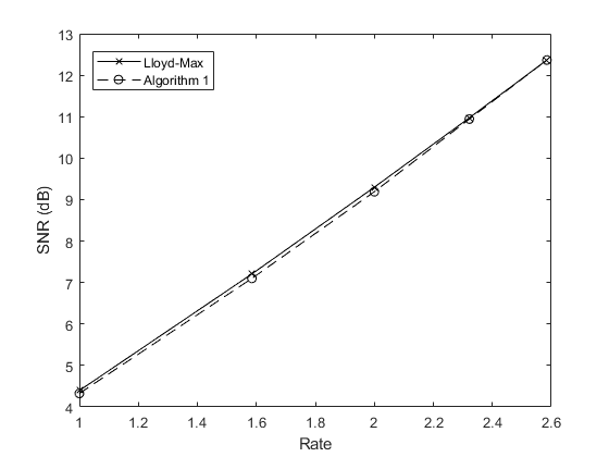
Figure 3: Comparison of Algorithm 1 with Lloyd-Max for i.i.d. Gaussian source

VII Conclusion

We presented a reinforcement learning based algorithm for the design of zero-delay codes for Markov sources. For finite alphabet sources we proved that our Q-learning based algorithm produces zero-delay codes that are optimal as the quantization of the underlying probability space becomes arbitrarily fine, provided the source starts from its invariant distribution. As far as we know, this is the first provably optimal design method for zero-delay coding. The performance of the algorithm was also demonstrated via simulations for finite alphabet as well as continuous sources.

In future work, we aim to rigorously show the near-optimality of our algorithm for continuous alphabet sources with the aid of the quantization scheme in [52, Section V.C], which we already used, in a heuristic way, in our simulations for a continuous source. Furthermore, we are working on generalizing the results to the case where the channel is noisy and the encoder has access to feedback from the channel; most results in our paper seem to go through in this case too, with only a slight modification of the MDP formulation and the update equations.

We are also currently investigating a modified Q-learning approach that uses a finite window of quantizers and quantizer outputs as the state of the code instead of the current belief $\pi_{t}$. The benefits of such an approach include simpler implementation, fewer computations, and an explicit performance bound in terms of the window length. The analysis for such codes becomes quite intricate due to the fact that the notion of predictor stability required for this method is stricter than that we used in this paper, motivating the study of alternative predictor stability conditions.

In the following, consider an MDP $(\mathsf{Z},\mathsf{U},P,c)$ and fix some state $z_{0}\in\mathsf{Z}$.

Assumption 4

1. $c$ is continuous, nonnegative, and bounded.

2. $\mathsf{Z}$ is a compact metric space.

3. $\mathsf{U}$ is as a compact metric space.

4. $P(\,\cdot\,|z,u)$ is weakly continuous in $(z,u)$.

5. The family of functions $\{h_{\beta}:\mathsf{Z}\to\mathbb{R},\;\beta\in(0,1)\}$, where $h_{\beta}(z)\coloneqq J^{*}_{\beta}(z)-J^{*}_{\beta}(z_{0})$ for some fixed $z_{0}\in\mathsf{Z}$, is uniformly bounded and equicontinuous.

The following is a standard result in the MDP literature, see e.g. [54, Theorem 3.8], [9, Theorem 5.4.3] for related results.

Lemma 8

[45, Theorems 7.3.3 and 7.3.4] Consider an MDP which satisfies Assumption 4. Then there exist a constant $g^{*}\geq 0$ and a measurable function $f:\mathsf{Z}\to\mathsf{U}$ such that the stationary policy $\gamma^{*}=\{f,f,\ldots\}$ is optimal for the average cost problem and $g^{*}$ is the optimal value function, i.e.,

$$g^{*}=J^{*}(z)=J(z,\gamma^{*})\text{\ \ for all $z\in\mathsf{Z}$.}$$

Furthermore, $g^{*}=\lim_{\beta\uparrow 1}(1-\beta)J^{*}_{\beta}(z)$.

Lemma 9

Let $g$ be a constant and $h:\mathsf{Z}\to\mathbb{R}$, $f:\mathsf{Z}\to\mathsf{U}$ be such that for all $z\in\mathsf{Z}$,

$$g+h(z)\geq c(z,f(z))+\int h(z^{\prime})P(dz^{\prime}|z,f(z))$$ (15)

and

$$\liminf_{n\to\infty}\frac{1}{n}\mathbf{E}^{\gamma}_{z}\left[h(z_{n})\right]\geq 0,$$ (16)

where $\gamma=\{f,f,\ldots\}$ and $\{z_{t}\}_{t\geq 0}$ is the state process under policy $\gamma$ and arbitrary given initial state $z\in\mathsf{Z}$. Then $g$ is an upper bound to the average cost of policy $\gamma$, i.e.,

$$J(z,\gamma)\leq g\text{ \ \ for all $z\in\mathsf{Z}$.}$$

Proof:

By the law of iterated expectation, we have

$$\mathbf{E}^{\gamma}_{z}\left[\sum_{t=1}^{n}h(z_{t})\right]=\mathbf{E}^{\gamma}_{z}\left[\sum_{t=1}^{n}\mathbf{E}^{\gamma}\left[h(z_{t})|z_{[0,t-1]},u_{[0,t-1]}\right]\right].$$

By the Markov property and (15),

$$\mathbf{E}^{\gamma}\left[h(z_{t})|z_{[0,t-1]},u_{[0,t-1]}\right] =\int h(z^{\prime})P(dz^{\prime}|z_{t-1},u_{t-1})$$

$$=c(z_{t-1},f(z_{t-1}))+\int h(z^{\prime})P(dz^{\prime}|z_{t-1},f(z_{t-1}))-c(z_{t-1},f(z_{t-1}))$$

$$\leq g+h(z_{t-1})-c(z_{t-1},f(z_{t-1})).$$

Substituting this into the previous equation, we obtain

$$\mathbf{E}^{\gamma}_{z}\left[\sum_{t=1}^{n}h(z_{t})\right]\leq\mathbf{E}^{\gamma}_{z}\left[\sum_{t=1}^{n}g+h(z_{t-1})-c(z_{t-1},f(z_{t-1}))\right].$$

Rearranging,

$$\mathbf{E}^{\gamma}_{z}\left[\sum_{t=1}^{n}c(z_{t-1},f(z_{t-1}))\right]\leq ng+h(z)-\mathbf{E}^{\gamma}_{z}\left[h(z_{n})\right].$$

Dividing by $n$ and taking the limsup,

$$J(z,\gamma)\leq g+\limsup_{n\to\infty}\left(-\frac{1}{n}\mathbf{E}^{\gamma}_{z}\left[h(z_{n})\right]\right)\leq g,$$

where we use (16) for the last inequality. ∎

The next result shows that if the discount factor $\beta$ is close enough to $1$, a policy that is optimal or near-optimal for the discounted cost, is also near-optimal in the average cost sense.

Theorem 5

Let Assumption 4 hold. Then for every $\epsilon>0$, there exists a $\beta\in(0,1)$ such that if a stationary policy $\gamma_{\beta}=\{f_{\beta},f_{\beta},\ldots\}$ satisfies for some $\delta\geq 0$,

$$J_{\beta}(z,\gamma_{\beta})\leq J^{*}_{\beta}(z)+\delta$$ (17)

for all $z\in\mathsf{Z}$, then

$$J(z,\gamma_{\beta})\leq g^{*}+\epsilon+(1-\beta)\delta$$

for all $z\in\mathsf{Z}$, where $g^{*}$ is the optimal average cost (which is constant by Lemma 8)

Proof:

As in Assumption 4, let $h_{\beta}(z)=J^{*}_{\beta}(z)-J^{*}_{\beta}(z_{0})$ and define $\hat{h}_{\beta}(z)\coloneqq J_{\beta}(z,\gamma_{\beta})-J^{*}_{\beta}(z_{0})$. We will verify that the conditions of Lemma 9 hold with $g=g^{*}+\epsilon+(1-\beta)\delta$, $h=\hat{h}_{\beta}$, and $f=f_{\beta}$. Indeed, for any $\beta\in(0,1)$,

$$\hat{h}_{\beta}(z)+g^{*}-(g^{*}-(1-\beta)J^{*}_{\beta}(z_{0}))+(1-\beta)\int\hat{h}_{\beta}(z^{\prime})P(dz^{\prime}|z,f_{\beta}(z))$$ (18)

$$=\hat{h}_{\beta}(z)+(1-\beta)J^{*}_{\beta}(z_{0})+(1-\beta)\int\hat{h}_{\beta}(z^{\prime})P(dz^{\prime}|z,f_{\beta}(z))$$

$$=\hat{h}_{\beta}(z)+(1-\beta)\int J_{\beta}(z^{\prime},\gamma_{\beta})P(dz^{\prime}|z,f_{\beta}(z))$$

$$=c(z,f_{\beta}(z))+\beta\int J_{\beta}(z^{\prime},\gamma_{\beta})P(dz^{\prime}|z,f_{\beta}(z))-J^{*}_{\beta}(z_{0})+(1-\beta)\int J_{\beta}(z^{\prime},\gamma_{\beta})P(dz^{\prime}|z,f_{\beta}(z))$$

$$=c(z,f_{\beta}(z))+\int\hat{h}_{\beta}(z^{\prime})P(dz^{\prime}|z,f_{\beta}(z)),$$

where the third equality follows from the identity

$$J_{\beta}(z,\gamma_{\beta})=c(z,f_{\beta}(z))+\beta\int J_{\beta}(z^{\prime},\gamma_{\beta})P(dz^{\prime}|z,f_{\beta}(z)).$$

Now consider the terms in (18). By Lemma 8, there exists some $\beta_{1}\in(0,1)$ such that

$$\left|g^{*}-(1-\beta)J^{*}_{\beta}(z_{0})\right|\leq\frac{\epsilon}{2}\text{ \ \ for all $\beta\in\left[\beta_{1},1\right)$.}$$ (19)

On the other hand, for any $\beta\in(0,1)$ choose $\gamma_{\beta}$ so that it is $\delta$-optimal, i.e., (17) holds. Then we have

$$\|\hat{h}_{\beta}\|_{\infty}\leq\sup_{z\in\mathsf{Z}}\left|J_{\beta}(z,\gamma_{\beta})-J^{*}_{\beta}(z)\right|+\|h_{\beta}\|_{\infty}\leq\delta+\|h_{\beta}\|_{\infty}$$

and therefore

$$\left|(1-\beta)\int\hat{h}_{\beta}(z^{\prime})P(dz^{\prime}|z,f_{\beta}(z))\right|\leq(1-\beta)(\delta+\|h_{\beta}\|_{\infty}).$$

By Assumption 4, $h_{\beta}$ is uniformly bounded over $\beta$, so there exists some $\beta_{2}\in(0,1)$ such that

$$\left|(1-\beta)\int\hat{h}_{\beta}(z^{\prime})P(dz^{\prime}|z,f_{\beta}(z))\right|\leq(1-\beta)\delta+\frac{\epsilon}{2}\text{\ \ for all $\beta\in\left[\beta_{2},1\right)$. }$$ (20)

Thus taking $\beta^{*}=\max\{\beta_{1},\beta_{2}\}$ in (19) and (20), we have for all $\beta\in\left[\beta^{*},1\right)$,

$$g^{*}+\epsilon+(1-\beta)\delta+\hat{h}_{\beta}(z) \geq c(z,f_{\beta}(z))+\int\hat{h}_{\beta}(z^{\prime})P(dz^{\prime}|z,f_{\beta}(z)).$$

Finally, since $\hat{h}_{\beta}$ is bounded, (16) is satisfied. Thus by Lemma 9,

$$J(z,\gamma_{\beta})\leq g^{*}+\epsilon+(1-\beta)\delta.$$

∎

Algorithm 2: Predictor Quantization[35, Algorithm 1]

1:$n\geq 1,\pi_{t}=(p_{1},\ldots,p_{m})$

2:for $i=1$ to $m$ do

3:  $k_{i}^{\prime}=\lfloor np_{i}+\frac{1}{2}\rfloor$

4:end for

5:$n^{\prime}=\sum_{i}k_{i}^{\prime}$

6:if $n=n^{\prime}$ then return $(\frac{k_{1}^{\prime}}{n},\ldots,\frac{k_{m}^{\prime}}{n})$

7:end if

8:for $i=1$ to $m$ do

9:  $\delta_{i}=k_{i}^{\prime}-np_{i}$

10:end for

11:Sort $\delta_{i}$ s.t. $\delta_{i_{1}}\leq\ldots\leq\delta_{i_{m}}$

12:$\Delta=n^{\prime}-n$

13:if $\Delta>0$ then

14:  $k_{i_{j}}=\begin{cases}k_{i_{j}}^{\prime}\quad&j=1,\ldots,m-\Delta\\ k_{i_{j}}^{\prime}-1\quad&j=m-\Delta+1,\ldots,m\end{cases}$

15:else

16:  $k_{i_{j}}=\begin{cases}k_{i_{j}}^{\prime}+1\quad&j=1,\ldots,|\Delta|\\ k_{i_{j}}^{\prime}\quad&j=|\Delta|+1,\ldots,m\end{cases}$

17:end if

18:return $(\frac{k_{1}}{n},\ldots,\frac{k_{m}}{n})$

Transition matrix of source in Figure 1

$$\begin{pmatrix}0.1331&0.0824&0.0311&0.2131&0.2623&0.0714&0.0417&0.1645\\ 0.1207&0.1501&0.1268&0.1974&0.0952&0.0862&0.1870&0.0362\\ 0.2320&0.0491&0.1770&0.1476&0.1530&0.1691&0.0215&0.05043\\ 0.0162&0.1930&0.2511&0.1935&0.0688&0.1280&0.0893&0.0597\\ 0.0420&0.1496&0.1130&0.0478&0.1073&0.2345&0.0692&0.2363\\ 0.1382&0.1720&0.1378&0.1369&0.0396&0.1923&0.1383&0.0445\\ 0.1710&0.2153&0.1579&0.0366&0.1530&0.1144&0.0439&0.1075\\ 0.1292&0.0534&0.1309&0.0315&0.2837&0.2617&0.0103&0.0988\end{pmatrix}.$$ (21)

Invariant distribution

$$\begin{pmatrix}0.1211&0.1326&0.1416&0.1328&0.1360&0.1580&0.0806&0.0973\end{pmatrix}.$$ (22)

References

- [1] H. S. Witsenhausen, “On the structure of real-time source coders,” Bell System Technical Journal, vol. 58, pp. 1437–1451, 1979.
- [2] J. C. Walrand and P. Varaiya, “Causal coding and control of Markov chains,” Systems & Control Letters, vol. 3, pp. 189 – 192, 1983.
- [3] D. Teneketzis, “On the structure of optimal real-time encoders and decoders in noisy communication,” IEEE Transactions on Information Theory, vol. 52, pp. 4017–4035, 2006.
- [4] A. Mahajan and D. Teneketzis, “Optimal design of sequential real-time communication systems,” IEEE Transactions on Information Theory, vol. 55, pp. 5317–5338, 2009.
- [5] S. Yüksel, “On optimal causal coding of partially observed Markov sources in single and multi-terminal settings,” IEEE Transactions on Information Theory, vol. 59, pp. 424–437, 2013.
- [6] T. Linder and S. Yüksel, “On optimal zero-delay quantization of vector Markov sources,” IEEE Transactions on Information Theory, vol. 60, pp. 2975–5991, 2014.
- [7] R. G. Wood, T. Linder, and S. Yüksel, “Optimal zero delay coding of Markov sources: Stationary and finite memory codes,” IEEE Transactions on Information Theory, vol. 63, pp. 5968–5980, 2017.
- [8] D. P. Bertsekas, Dynamic Programming and Stochastic Optimal Control. New York, New York: Academic Press, 1976.
- [9] O. Hernández-Lerma and J. B. Lasserre, Discrete-Time Markov Control Processes: Basic Optimality Criteria. Springer, 1996.
- [10] C. Szepesvari, Algorithms for Reinforcement Learning. Springer, 2010.
- [11] S. Tatikonda and S. Mitter, “The capacity of channels with feedback,” IEEE Transactions on Information Theory, vol. 55, no. 1, pp. 323–349, 2009.
- [12] M. Ghomi, T. Linder, and S. Yüksel, “Zero-delay lossy coding of linear vector Markov sources: Optimality of stationary codes and near optimality of finite memory codes,” IEEE Transactions on Information Theory, vol. 68, no. 5, pp. 3474–3488, 2021.
- [13] C. J. C. H. Watkins and P. Dayan, “Q-learning,” Machine Learning, vol. 8, pp. 279–292, 1992.
- [14] J. N. Tsitsiklis, “Asynchronous stochastic approximation and Q-learning,” Machine Learning, vol. 16, pp. 185–202, 1994.
- [15] W. L. Baker, “Learning via stochastic approximation in function space,” Ph.D. dissertation, Harvard University, Cambridge, MA, 1997.
- [16] C. Szepesvári and M. Littman, “A unified analysis of value-function-based reinforcement-learning algorithms.” Neural computation, vol. 11, no. 8, pp. 2017–2060, 1999.
- [17] D. P. Bertsekas and J. N. Tsitsiklis, Neuro-Dynamic Programming. Belmont, MA: Athena Scientific, 1996.
- [18] A. Kara, N. Saldi, and S. Yüksel, “Q-learning for MDPs with general spaces: Convergence and near optimality via quantization under weak continuity,” Journal of Machine Learning Research, vol. 24, no. 199, pp. 1–34, 2023.
- [19] E. I. Silva, M. S. Derpich, and J. Østergaard, “A framework for control system design subject to average data-rate constraints,” IEEE Transactions on Automatic Control, vol. 56, pp. 1886–1899, August 2011.
- [20] E. Silva, M. Derpich, J. Østergaard, and M. Encina, “A characterization of the minimal average data rate that guarantees a given closed-loop performance level,” IEEE Transactions on Automatic Control, vol. 61, no. 8, pp. 2171–2186, 2015.
- [21] P. Stavrou, J. Østergaard, and C. Charalambous, “Zero-delay rate distortion via filtering for vector-valued Gaussian sources,” IEEE Journal of Selected Topics in Signal Processing, vol. 12, no. 5, pp. 841–856, 2018.
- [22] T. Cuvelier, T. Tanaka, and R. H. Jr., “Time-invariant prefix coding for LQG control,” arXiv preprint arXiv:2204.00588, 2022.
- [23] R. Bansal and T. Başar, “Simultaneous design of measurement and control strategies in stochastic systems with feedback,” Automatica, vol. 45, pp. 679–694, September 1989.
- [24] S. Tatikonda, A. Sahai, and S. Mitter, “Stochastic linear control over a communication channels,” IEEE Transactions on Automatic Control, vol. 49, pp. 1549–1561, September 2004.
- [25] T. Tanaka, K. Kim, P. Parrilo, and S. Mitter, “Semidefinite programming approach to Gaussian sequential rate-distortion trade-offs,” IEEE Transactions on Automatic Control, vol. 62, no. 4, pp. 1896–1910, 2016.
- [26] M. Derpich and J. Østergaard, “Improved upper bounds to the causal quadratic rate-distortion function for Gaussian stationary sources,” IEEE Transactions on Information Theory, vol. 58, no. 5, pp. 3131–3152, 2012.
- [27] P. Stavrou and M. Skoglund, “Asymptotic reverse waterfilling algorithm of NRDF for certain classes of vector Gauss-Markov processes,” IEEE Transactions on Automatic Control, vol. 67, no. 6, pp. 3196–3203, 2022.
- [28] P. Stavrou, T. Tanaka, and S. Tatikonda, “The time-invariant multidimensional Gaussian sequential rate-distortion problem revisited,” IEEE Transactions on Automatic Control, vol. 65, no. 5, pp. 2245–2249, 2019.
- [29] V. Kostina and B. Hassibi, “Rate-cost tradeoffs in control,” IEEE Transactions on Automatic Control, vol. 64, no. 11, pp. 4525–4540, 2019.
- [30] D. Pollard, “Quantization and the method of -means,” IEEE Transactions on Information Theory, vol. 28, pp. 199–205, 1982.
- [31] T. Linder, G. Lugosi, and K. Zeger, “Rates of convergence in the source coding theorem, in empirical quantizer design, and in universal lossy source coding,” IEEE Transactions on Information Theory, vol. 40, no. 6, pp. 1728–1740, 1994.
- [32] T. Linder, “Learning-theoretic methods in vector quantization,” in Principles of nonparametric learning. Springer, Wien, New York, 2002, pp. 163–210.
- [33] D. Gündüz, P. de Kerret, N. Sidiropoulos, D. Gesbert, C. Murthy, and M. van der Schaar, “Machine learning in the air,” IEEE Journal on Selected Areas in Communications, vol. 37, no. 10, pp. 2184–2199, 2019.
- [34] A. Gersho and R. Gray, Vector Quantization and Signal Compression. Springer New York, 2012.
- [35] Y. Reznik, “An algorithm for quantization of dicrete probability distributions,” DCC 2011, pp. 333–342, 2011.
- [36] S. Yüksel and T. Linder, “Optimization and convergence of observation channels in stochastic control,” SIAM Journal on Control and Optimization, vol. 50, pp. 864–887, 2012.
- [37] N. Saldi, T. Linder, and S. Yüksel, Finite Approximations in Discrete-Time Stochastic Control: Quantized Models and Asymptotic Optimality. Birkhäuser, 2018.
- [38] A. Kara and S. Yüksel, “Convergence of finite memory Q-learning for POMDPs and near optimality of learned policies under filter stability,” Mathematics of Operations Research, vol. 48, pp. 2066–2093, 2023.
- [39] N. Saldi, S. Yüksel, and T. Linder, “On the asymptotic optimality of finite approximations to Markov decision processes with Borel spaces,” Mathematics of Operations Research, vol. 42, no. 4, pp. 945–978, 2017.
- [40] P. Chigansky and R. Liptser, “Stability of nonlinear filters in non-mixing case,” Annals of Applied Probability, vol. 14, pp. 2038–2056, 2004.
- [41] C. McDonald and S. Yüksel, “Stochastic observability and filter stability under several criteria,” IEEE Transactions on Automatic Control, to be published. doi: 0.1109/TAC.2023.3302208.
- [42] R. van Handel, “The stability of conditional Markov processes and Markov chains in random environments,” Annals of Applied Probability, vol. 37, pp. 1876–1925, 2009.
- [43] L. Stettner, “Ergodic control of partially observed Markov control processes with equivalent transition probabilities,” Applicationes Mathematicae, vol. 22, pp. 25–38, 1993.
- [44] O. Hernández-Lerma and J. B. Lasserre, Markov chains and invariant probabilities. Basel: Birkhäuser-Verlag, 2003.
- [45] S. Yüksel. (2023) Optimization and control of stochastic systems. [Online]. Available: https://mast.queensu.ca/~yuksel/LectureNotesOnStochasticOptControl.pdf
- [46] R. L. Dobrushin, “Central limit theorem for nonstationary Markov chains. I,” Theory of Probability & Its Applications, vol. 1, no. 1, pp. 65–80, 1956.
- [47] M. Hairer. (2010) Convergence of Markov processes. [Online]. Available: https://www.hairer.org/notes/Convergence.pdf
- [48] C. Villani, Optimal transport: old and new. Springer, 2008.
- [49] E. Even-Dar and Y. Mansour, “Learning rates for Q-learning,” Journal of Machine Learning Research, vol. 5, pp. 1–25, 2004.
- [50] S. Lloyd, “Least squares quantization in PCM,” IEEE Transactions on Information Theory, vol. 28, no. 2, pp. 129–137, 1982.
- [51] W. Kreitmeier, “Optimal vector quantization in terms of Wasserstein distance,” Journal of Multivariate Analysis, vol. 102, no. 8, pp. 1225–1239, 2011.
- [52] N. Saldi, S. Yüksel, and T. Linder, “Finite model approximations for partially observed Markov decision processes with discounted cost,” IEEE Transactions on Automatic Control, vol. 65, 2020.
- [53] J. Kieffer, “Uniqueness of locally optimal quantizer for log-concave density and convex error weighting function,” IEEE Transactions on Information Theory, vol. 29, no. 1, pp. 42–47, 1983.
- [54] M. Schal, “Average optimality in dynamic programming with general state space,” Mathematics of Operations Research, vol. 18, no. 1, pp. 163–172, 1993.