Optimal Functional Bilinear Regression with Two-way Functional Covariates via Reproducing Kernel Hilbert Space

Abstract

Traditional functional linear regression usually takes a one-dimensional functional predictor as input and estimates the continuous coefficient function. Modern applications often generate two-dimensional covariates, which become matrices when observed at grid points. To avoid the inefficiency of the classical method involving estimation of a two-dimensional coefficient function, we propose a functional bilinear regression model, and introduce an innovative three-term penalty to impose roughness penalty in the estimation. The proposed estimator exhibits minimax optimal property for prediction under the framework of reproducing kernel Hilbert space. An iterative generalized cross-validation approach is developed to choose tuning parameters, which significantly improves the computational efficiency over the traditional cross-validation approach. The statistical and computational advantages of the proposed method over existing methods are further demonstrated via simulated experiments, the Canadian weather data, and a biochemical long-range infrared light detection and ranging data.

Keywords: Functional principal component analysis; Functional linear regression; Tensor regression; Scalar-on-image regression; Minimax optimality.

1 Introduction

The functional linear regression (FLR) is a powerful approach for predicting a scalar response from a one-dimensional functional predictor. It was first introduced by Ramsay and Dalzell (1991), and has been widely used in functional data analysis since then (Ramsay and Silverman, 2002, 2005a; Reiss et al., 2017; Wang et al., 2016). Consider a scalar response $Y$ and a square integrable random function $X(\cdot)$ with mean $0$ defined over the domain $\mathcal{T}$, the FLR model adopts the following form,

$$Y=\mu_{0}+\int_{\mathcal{T}}X(t)\beta_{0}(t)~{}dt+\epsilon,$$ (1)

where $\mu_{0}$ is the intercept, $\beta_{0}(\cdot)$ is the unknown coefficient function, and $\epsilon$ is zero-mean noise.

The predictor $X(\cdot)$ in Model (1) is often one-dimensional, and is therefore sometimes referred to as one-way functional input. However, in recent years, there has been an increasing amount of data collected in a two-way fashion. For instance, the functional magnetic resonance imaging (fMRI) data may be viewed as the function of blood-oxygen-level dependent contrast observed for the whole brain over time and the data can be used to predict the severity of the attention deficit hyperactivity disorder. Besides neuroimaging, such two-way functional data are now frequently encountered in fields like finance, economics, social science, and so on. To be more specific, the random predictor $X(\cdot)$ in these cases is a bivariate function defined on domain $\mathcal{T}_{1}\times\mathcal{T}_{2}$.

To generalize Model (1), we propose the following functional bilinear regression (FBLR) model,

$$Y=\mu_{0}+\int_{\mathcal{T}_{1}\times\mathcal{T}_{2}}\alpha_{0}(s)X(s,t)\beta_{0}(t)~{}dsdt+\epsilon.$$ (2)

Here, $Y$, $\mu_{0}$ and $\epsilon$ are again the scalar response, intercept, and error terms respectively, $X(\cdot,\cdot)$ is a square integrable bivariate function defined on $\mathcal{T}_{1}\times\mathcal{T}_{2}$, and $\alpha_{0}(\cdot)$ on domain $\mathcal{T}_{1}$ and $\beta_{0}(\cdot)$ on $\mathcal{T}_{2}$ are two unknown coefficient functions. The error term $\epsilon$ is assumed to have mean 0 and finite variance. The goal of the FBLR is to recover $\alpha_{0}(\cdot)$ and $\beta_{0}(\cdot)$ from $n$ independent and identically distributed training sample $\{x_{i}(\cdot,\cdot),y_{i}\}_{i=1}^{n}$ and make predictions for testing observations accordingly.

A few articles have examined the problem of regression with two-way functional predictor as summarized in Happ et al. (2018). Reiss and Ogden (2010) studied this problem with 2D images as predictors by regressing on the principal component (PC) scores obtained from two-dimensional principal component analysis (PCA) of the observed images. Sangalli et al. (2013) proposed to penalize with the integral of the square of the Laplacian of the two-dimensional coefficient function. Guillas and Lai (2010) approached the problem through fixed bivariate spline. Wang et al. (2014) and Reiss et al. (2015) transformed the multi-dimensional functional problem into estimation of wavelet coefficient via wavelet transformation. Kang et al. (2018) investigated this problem from a Bayesian perspective.

These aforementioned papers considered the following model

$$Y=\mu_{0}+\int_{\mathcal{T}_{1}\times\mathcal{T}_{2}}X(s,t)\beta_{0}(s,t)~{}dsdt+\epsilon,$$ (3)

and focused on the estimation of the coefficient function $\beta_{0}(\cdot,\cdot)$. Few have studied the theoretical properties of the proposed estimator.

The key difference among Models (1), (2) and (3) is that our Model (2) adopts two one-dimensional coefficient functions compared to a single one-dimensional coefficient function in Model (1) or a single two-dimensional coefficient function in Model (3). Model (2) is a special case of Model (3). The primary motivation is that for many applications, the first and second dimensions of the covariate $X(\cdot,\cdot)$ may be for different domains, and hence their effects might as well be decoupled. For instance, in the fMRI data, two functions should correspond to the spatial and temporal effects respectively. In Section 5 on the Canadian weather data, the two functions correspond to the time-of-the-day and day-of-the-year effects. In Appendix G on the biochemical application, the two functions are for range and wavelength effects respectively.

The second motivation is dimension reduction: even if the two dimensions of the predictor correspond to the same domain such as in images, the estimation in Model (2) might be more efficient than that in (3). In addition, compared with Model (1), the two coefficient functions in Model (2) preserves the two-way functional structural information through a bilinear form, $\alpha_{0}(s)X(s,t)\beta_{0}(t)$. In the literature, this type of bilinear/multilinear combination is becoming increasingly common when dealing with two-way/multi-way data (e.g., Dyrholm et al., 2007; Zhou et al., 2013; Bi et al., 2018, 2021; Chen et al., 2022).

The last motivation is that even if the true coefficient function is intrinsically two-dimensional, sometimes, it can be approximated by the sum of a few terms such as $\beta_{0}(s,t)=\sum_{r=1}^{R}\alpha_{0}^{[r]}(s)\beta_{0}^{[r]}(t),$ which resembles the continuous version of the singular value decomposition (SVD). This approximation leads to the following model

$$Y=\mu_{0}+\sum_{r=1}^{R}\int_{\mathcal{T}_{1}\times\mathcal{T}_{2}}\alpha_{0}^{[r]}(s)X(s,t)\beta_{0}^{[r]}(t)~{}dsdt+\epsilon.$$ (4)

Suppose one can estimate Model (2) via some approach, then Model (4) can be estimated in an iterative fashion: apply the approach to the original data $\{x_{i}(\cdot,\cdot),y_{i}\}_{i=1}^{n}$, obtain the estimate $\hat{\alpha}_{0}^{[1]}(s)\hat{\beta}_{0}^{[1]}(t)$ and retain the residuals $\{e_{i}\}_{i=1}^{n}$; re-apply the approach to the predictors and residuals $\{x_{i}(\cdot,\cdot),e_{i}\}_{i=1}^{n}$, obtain the estimate $\hat{\alpha}_{0}^{[2]}(s)\hat{\beta}_{0}^{[2]}(t)$ and retain the updated residuals; and repeat.

A naive and straightforward approach to deal with the two-way functional covariate is to convert the two-dimensional predictor into one-dimensional through stacking the data along one direction, then followed by implementing the traditional FLR Model (1). However, this conversion would destroy the two-way functional structure of the covariate, and the resulting one-way predictor is typically no longer a smooth function, which violates the underlying assumption of FLR. Therefore, adopting Model (1) is not a good choice for a two-dimensional functional predictor.

Although the extension from linear to bilinear seems natural, the generalization is in fact non-trivial. Due to the interplay of the two coefficient functions in a product form, several challenges arise from the design of the penalty, the development of the algorithm, and the theoretical analysis. Therefore, the five-fold main contributions are elaborated below.

First, there are mainly two categories of approaches for FLR, including functional PCA regression (FPCR) (e.g., Ramsay and Silverman, 2002, 2005a; Cai and Hall, 2006) and smoothness penalization under the framework of reproducing kernel Hilbert space (RKHS) (e.g., Yuan and Cai, 2010; Cai and Yuan, 2012).  Cai and Yuan (2012) show that the penalty approach has an advantage over FPCR, because the penalty approach does not require the alignment of the reproducing kernel and the covariance kernel of the predictor, while the FPCR approach does. Hence, we take the penalty approach for the FBLR problem when extending from 1D to 2D. Our key innovation is the proposal of a three-term penalty that involves the Hilbert norm based on the reproducing kernel and the norm associated with the covariance kernel. This three-term penalty enjoys the invariant property and successfully separates the effects from the smoothness levels of the two coefficient functions $\alpha(\cdot)$ and $\beta(\cdot)$, which leads to a minimax rate optimal solution.

Second, upon the proposal of the penalty function, an iterative algorithm is developed to optimize the objective function because of the bi-convexity of the function. The main idea for the block descent algorithm is to reduce the two-way problem into a one-way FLR problem in each iteration, which can then be solved by the representer theorem (Wahba, 1990), with slight complications since the one-way problem involves updated 1D stochastic processes and reproducing kernels. Furthermore, there are two tuning parameters in the penalty corresponding to the different degrees of smoothness of the two coefficient functions. Naive cross validation (CV) over two-dimensional grid is outrageously time-consuming. A novel iterative generalized cross validation (iGCV) approach is proposed whose computational time is only slightly more than the iterative FBLR algorithm with fixed tuning parameters, while achieving similar performance as the computationally expensive CV.

Third, one interesting finding is that the minimax convergence rate for the FBLR is identical to that of the FLR if we assume the domains, kernels and covariances are the same for the two dimensions of the two-way functional data. Unlike the FLR problem, whose solution is explicit and can be directly analyzed theoretically, the FBLR problem does not have an explicit solution since the two coefficient functions interact with each other. Therefore, the techniques from Cai and Yuan (2012) cannot be applied. To prove the minimax property, we need to combine 2D linearization, two-dimensional Gâteaux derivatives with sophisticated expressions, block matrix inversion, and RKHS, among others.

Fourth, this article serves as the first attempt to study the theoretical properties of scalar-on-matrix functional regression with low rank assumption, where the two-dimensional coefficient function has low rank of products of one-dimensional coefficient functions. Such low rank assumption is helpful to extend to functional tensor predictor of even higher order in the future. Tensor regression has become increasingly important recently. There are different combinations of response types and predictor types motivated by various applications, such as tensor-on-vector regression (e.g., Sun and Li, 2017; Zhou et al., 2021), scalar-on-tensor regression (e.g., Zhou et al., 2013; Liu et al., 2019), and tensor-on-tensor regression (e.g., Hoff, 2015; Chen et al., 2021). Most of the existing work focus on the low tensor rank assumption on the coefficient tensor with or without sparsity assumption. To the best of our knowledge, work on functional matrix or tensor predictor is very rare.

Lastly, we apply FBLR to two real data examples. One is the Canadian weather data, a well-known example in the functional data analysis (FDA) literature. The goal is to predict precipitation at different weather stations with temperature information. The existing FDA studies (e.g., Ramsay and Dalzell, 1991; Ramsay and Silverman, 2005b; Cai and Yuan, 2012) focus on 1D PCA in Model (1), where each observation is a vector of 365 daily average temperatures. Besides daily variation, we introduce 2D predictors with the second domain reflecting the hourly temperature variation in Model (3). The extra domain not only boosts the prediction accuracy, but also echos some meteorological phenomena. The other real data example is the Light Detection and Ranging (LIDAR) data from the biochemistry field (Xun et al., 2013). The data generating process naturally produces smooth data and call for FDA method. For both datasets, FBLR and its iterative variant have higher prediction accuracy and better interpretability compared to existing 2D FLR and 1D FLR methods.

The rest of the paper is organized as follows. A brief review of FLR and the methodology for FBLR are provided in Section 2. The optimal theoretical property of the proposed method is discussed in Section 3. Simulation and the Canadian data analysis are presented in Sections 4 and 5. Section 6 concludes with discussion. All proofs, more simulation results, and the biochemical data application are provided in the supplementary materials.

2 Methodology

2.1 Notation and definitions

Suppose that $\mathcal{T}$ is a compact set. We denote by $\mathcal{H}(K)$ an RKHS associated with the reproducing kernel $K$, $\langle\cdot,\cdot\rangle_{K}$ the associated inner product, and $\|\cdot\|_{K}$ the induced norm. Then, we have $K(s,\cdot)\in\mathcal{H}(K)$ for all $s\in\mathcal{T}$ and $f(t)=\langle K(t,\cdot),f\rangle_{K}$ for all $f\in\mathcal{H}(K)$. We refer the readers to Wahba (1990), Gu (2013) and references therein for more details. Let $K_{1}(\cdot,\cdot):\mathcal{T}_{1}\times\mathcal{T}_{1}\mapsto\mathbb{R}$ and $K_{2}(\cdot,\cdot):\mathcal{T}_{2}\times\mathcal{T}_{2}\mapsto\mathbb{R}$ be two reproducing kernels, and $\mathcal{H}(K_{1})$ and $\mathcal{H}(K_{2})$ be the corresponding RKHS’s. The coefficients $\alpha_{0}(\cdot)$ and $\beta_{0}(\cdot)$ of Model (2) reside in $\mathcal{H}(K_{1})$ and $\mathcal{H}(K_{2})$, respectively.

The covariance function of the mean zero bivariate random function $X(\cdot,\cdot)$ plays another important role in developing both methodology and theory of FBLR. We define it as $C(s_{1},t_{1},s_{2},t_{2})=\mathbb{E}[X(s_{1},t_{1})X(s_{2},t_{2})]$, for any $s_{1},s_{2}\in\mathcal{T}_{1}$ and $t_{1},t_{2}\in\mathcal{T}_{2}$. As mentioned earlier, the two dimensions of $X(\cdot,\cdot)$ usually correspond to different domains, and hence the covariance can be reasonably assumed to have a decomposable or separable structure, that is, $C(s_{1},t_{1},s_{2},t_{2})=C_{\alpha}(s_{1},s_{2})C_{\beta}(t_{1},t_{2})$, where $C_{\alpha}(\cdot,\cdot)$ and $C_{\beta}(\cdot,\cdot)$ are two real bivariate functions that characterize the covariance structures along the first and second dimensions respectively. We note that this type of decomposable covariance structure has been widely used in the literature recently when dealing with two-way data (e.g., Zhou, 2014; Volfovsky and Hoff, 2015; Hafner et al., 2020; Aston et al., 2017; Chen et al., 2021, 2023). Similar to the reproducing kernels $K_{1}$ and $K_{2}$, the two covariance functions $C_{\alpha}$ and $C_{\beta}$ are also symmetric and nonnegative definite. The subscripts $\alpha$ and $\beta$ will be used frequently to differentiate between the two dimensions.

Lastly, for any $f\in\mathcal{H}(K_{1})$ and $g\in\mathcal{H}(K_{2})$, we define two semi-norms as follows,

$$\begin{split}\|f\|_{0\alpha}&=\left(\int_{\mathcal{T}_{1}\times T_{1}}f(s_{1})C_{\alpha}(s_{1},s_{2})f(s_{2})ds_{1}ds_{2}\right)^{1/2},\\ \|g\|_{0\beta}&=\left(\int_{\mathcal{T}_{2}\times T_{2}}g(t_{1})C_{\beta}(t_{1},t_{2})g(t_{2})dt_{1}dt_{2}\right)^{1/2}.\end{split}$$ (5)

They will appear in the penalty term of the regularization approach and play a crucial role in the development of the asymptotic theory. It can be verified that the variance of the integral of the bilinear form in Model (2) is equal to the square of the product of the two norms defined above,

$$\mathbb{E}\left(\int_{\mathcal{T}_{1}\times\mathcal{T}_{2}}f(s)X(s,t)g(t)dsdt\right)^{2}=\|f\|_{0\alpha}^{2}\|g\|_{0\beta}^{2}.$$ (6)

2.2 Review of the smoothness regularization approach for one-way FLR

We provide a brief review of the smoothness regularization approach for the FLR model (1) in this section to facilitate discussion of FBLR. For more details, please see Yuan and Cai (2010), Cai and Yuan (2012), and references therein.

Consider the reproducing kernel $K(\cdot,\cdot)$ and the corresponding RKHS $\mathcal{H}(K)$. Assume that the coefficient function in Model (1) belongs to $\mathcal{H}(K)$. The smoothness regularized estimator can be obtained via minimizing the following objective with loss and penalty,

$$\widehat{\beta}=\operatorname*{arg\,min}_{\beta\in\mathcal{H}(K)}\ell_{n\lambda}(\beta)\stackrel{{\scriptstyle def}}{{=}}\operatorname*{arg\,min}_{\beta\in\mathcal{H}(K)}\left\{\ell_{n}(\beta)+\lambda J(\beta)\right\},$$ (7)

where $\ell_{n}(\beta)=n^{-1}\sum_{i=1}^{n}\left(y_{i}-\int_{\mathcal{T}}x_{i}(t)\beta(t)dt\right)^{2}$ is the normalized residual sum of squares measuring the goodness-of-fit, $J(\beta)={\|\beta\|_{K}^{2}}$ is the squared RKHS norm measuring the smoothness, and $\lambda$ is a tuning parameter that balances the trade-off between them.

Although the optimization in (7) is taken over an infinite-dimensional space, it can be solved by the representer theorem, i.e., Theorem 1 in Yuan and Cai (2010). This representer theorem is a generalization of the well-known representer lemma for smoothing splines (Wahba, 1990). The optimizer of (7) then has the following expression,

$$\widehat{\beta}(t)=\sum_{i=1}^{n}c_{i}\int_{\mathcal{T}}K(s,t)x_{i}(s)ds,$$ (8)

where the unknown scalars $c_{1},c_{2},\ldots,c_{n}\in\mathbb{R}$ can be readily computed once (8) is plugged back into (7), which leads to a quadratic function of $c_{1},...,c_{n}$. Please refer to Section 2 of Yuan and Cai (2010) for the details on the explicit expression and implementation.

2.3 Objective function of two-way FBLR

The smoothness regularization approach of the one-way FLR can be extended to the two-way FBLR. Assume that the coefficient function $\alpha_{0}$ resides in $\mathcal{H}(K_{1})$ and $\beta_{0}$ in $\mathcal{H}(K_{2})$, it is natural to estimate them by minimizing the following objective function,

$$(\widehat{\alpha},\widehat{\beta})=\operatorname*{arg\,min}_{\alpha\in\mathcal{H}(K_{1}),\beta\in\mathcal{H}(K_{2})}\ell_{n\lambda}(\alpha,\beta)\stackrel{{\scriptstyle def}}{{=}}\operatorname*{arg\,min}_{\alpha\in\mathcal{H}(K_{1}),\beta\in\mathcal{H}(K_{2})}\left\{\ell_{n}(\alpha,\beta)+J(\alpha,\beta)\right\}.$$ (9)

This is a direct analogy of (7). The first part, $\ell_{n}(\alpha,\beta)=n^{-1}\sum_{i=1}^{n}\left(y_{i}-\int_{\mathcal{T}_{1}\times\mathcal{T}_{2}}\alpha(s)x_{i}(s,t)\beta(t)dsdt\right)^{2}$, is again the data fidelity term. The second part of the penalty is defined as $J(\alpha,\beta)=\lambda_{\alpha}{\|\alpha\|_{K_{1}}^{2}}\|\beta\|_{0\beta}^{2}+\lambda_{\beta}\|\alpha\|_{0\alpha}^{2}{\|\beta\|_{K_{2}}^{2}}+\lambda_{\alpha}\lambda_{\beta}{\|\alpha\|_{K_{1}}^{2}}{\|\beta\|_{K_{2}}^{2}}$.

Such a penalty has the following desirable properties: First, the functions $\alpha$ and $\beta$ are only identifiable up to a scalar since $\alpha(s)X(s,t)\beta(t)=[c\alpha(s)]X(s,t)[c^{-1}\beta(t)]$ for any non-zero constant $c$. Therefore, the penalty is scale-invariant. Second, the loss term $\ell_{n}(\alpha,\beta)$ in (9) is bi-quadratic in $(\alpha,\beta)$. Hence, the penalty part is bi-quadratic. Third, ${\|\alpha\|_{K_{1}}^{2}}$ and ${\|\beta\|_{K_{2}}^{2}}$ appear to encourage smoothness. Fourth, setting one of $\lambda_{\alpha},\lambda_{\beta}$ to be zero can reduce the objective function to 1D FLR problem. Fifth, one can complete the squares in the loss $\ell_{n\lambda}(\alpha,\beta)$, let the sample size go to infinity, retain the terms relevant to $\alpha$ and $\beta$, and combine with Candidate 3 for the penalty $J(\alpha,\beta)$. As a result, the objective function (9) will lead to the following expansion $\|\alpha\|_{0\alpha}^{2}\|\beta\|_{0\beta}^{2}+\lambda_{\alpha}{\|\alpha\|_{K_{1}}^{2}}\|\beta\|_{0\beta}^{2}+\lambda_{\beta}\|\alpha\|_{0\alpha}^{2}{\|\beta\|_{K_{2}}^{2}}+\lambda_{\alpha}\lambda_{\beta}{\|\alpha\|_{K_{1}}^{2}}{\|\beta\|_{K_{2}}^{2}}=\left(\|\alpha\|_{0\alpha}^{2}+\lambda_{\alpha}{\|\alpha\|_{K_{1}}^{2}}\right)\left(\|\beta\|_{0\beta}^{2}+\lambda_{\beta}{\|\beta\|_{K_{2}}^{2}}\right)$, in which the first term comes from (6). Here, $\alpha$ and $\beta$ are completely decoupled and can have unrelated levels of smoothness. Note that the phenomenon of decoupling occurs only because of the special design of the penalty and the definition of the norm in (5). Adopting other choices will not simultaneously satisfy the invariant, bi-quadratic, specialization to 1D FLR, and decoupling requirements. See Appendix D for discussions on other choices of the penalty functions.

We comment that other three-term penalties have been used in the context of singular value decomposition of two-way functional data (Huang et al., 2009) and bivariate smoothing (Xiao et al., 2013). However, the penalty in Huang et al. (2009) only involves the standard $l_{2}$ norm of a vector and the norm of second order differences, which is a discrete version of $\left(\int(f^{\prime\prime})^{2}\right)$, and the penalty in Xiao et al. (2013) involves spline basis and differencing matrix, while our penalty involves the relatively more complicated norm defined in (5) and the Hilbert norm in a more general framework.

2.4 Optimization algorithm of two-way FBLR

Recall that the objective function is defined as follows, The bi-quadratic property of the function naturally calls for the block-descent algorithm to optimize the function iteratively. Given a starting point $\alpha^{(0)}$, one can iterate between minimizing one of $\alpha$ and $\beta$ while holding the other fixed until convergence. For the rest of this section, the focus will be on the discussion of how to update $\beta$ given $\alpha$ at each iteration. The updating rule for $\alpha$ given $\beta$ can be obtained analogously.

For any integer $k\geq 1$, suppose the estimation of $\alpha$ in the $(k-1)$th step is $\alpha^{(k-1)}$. Denote a new 1D random input function

$$\tilde{x}_{i}(t)=\int_{\mathcal{T}_{1}}\alpha^{(k-1)}(s)x_{i}(s,t)ds,$$ (10)

and for any $f\in\mathcal{H}(K_{2})$, define,

$${\|f\|_{\tilde{K}_{2}}^{2}}=\left(\lambda_{\alpha}{\|\alpha^{(k-1)}\|_{K_{1}}^{2}}\right)\|f\|_{0\beta}^{2}+\left(\lambda_{\beta}\|\alpha^{(k-1)}\|_{0\alpha}^{2}+\lambda_{\alpha}\lambda_{\beta}{\|\alpha^{(k-1)}\|_{K_{1}}^{2}}\right){\|f\|_{K_{2}}^{2}},$$ (11)

where, given $\alpha^{(k-1)}$, the terms $\lambda_{\alpha}{\|\alpha^{(k-1)}\|_{K_{1}}^{2}}$ and $\lambda_{\beta}\|\alpha^{(k-1)}\|_{0\alpha}^{2}+\lambda_{\alpha}\lambda_{\beta}{\|\alpha^{(k-1)}\|_{K_{1}}^{2}}$ are both known constants. Throughout this paper, we assume that $\|f\|_{0\alpha}^{2}\neq 0$ and $\|f\|_{0\beta}^{2}\neq 0$ hold for any $f$ that belongs to the null space of $K_{1}$ or $K_{2}$ and $f\neq 0$. This assumption is necessary to guarantee that the minimizer of $\mathbb{E}\ell_{n\lambda}(\alpha,\beta)$ is unique even when the optimization is constrained to the null space of $K_{1}$ or $K_{2}$. It then follows that ${\|\cdot\|_{\tilde{K}_{2}}}$ is a norm since ${\|f\|_{\tilde{K}_{2}}^{2}}=0$ if and only if $f=0$ and ${\|f\|_{\tilde{K}_{2}}^{2}}$ is quadratic. We further let $\tilde{K}_{2}(\cdot,\cdot)$ be the reproducing kernel associated with the norm ${\|\cdot\|_{\tilde{K}_{2}}}$.

Given $\alpha^{(k-1)}$, a new one-dimensional predictor (10) and a new kernel (11), the objective function $\ell_{n\lambda}(\alpha,\beta)$ for the $k$-th step becomes a functional of $\beta$ alone, denoted by $\ell_{n\lambda}(\beta;\alpha^{(k-1)})$, and can be re-expressed in a compact form,

$$\ell_{n\lambda}(\beta;\alpha^{(k-1)})=n^{-1/2}\sum_{i=1}^{n}\left(y_{i}-\int_{\mathcal{T}_{2}}\tilde{x}_{i}(t)\beta(t)dt\right)^{2}+1\times\|\beta\|_{\tilde{K}_{2}}^{2}.$$ (12)

The above objective function (12) is the same as the 1D FLR objective function (7) with inputs $\{(\tilde{x}_{i}(\cdot),y_{i})\}_{i=1}^{n}$, kernel $\tilde{K}_{2}(\cdot,\cdot)$, and tuning parameter $\lambda=1$. In other words, by fixing $\alpha^{(k-1)}$, the FBLR problem degenerates to an FLR problem with respect to $\beta$. Hence, the intermediate $\beta^{(k)}$ can be obtained from the 1D FLR via the representer theorem (8).

To summarize, the complete approach to obtain the estimators of FBLR is schematically presented in Algorithm 1 with given initialization, known covariance structure of the predictor, and fixed tuning parameters. Some details of the initialization, covariance structure, and tuning parameter selection are provided below.

Input:

1. The observations $(x_{i}(\cdot,\cdot),y_{i}),i=1,...,n$; initial estimator $\alpha^{(0)}$;

2. Penalty parameters $\lambda_{\alpha}$ and $\lambda_{\beta}$; reproducing kernels $K_{1}$ and $K_{2}$;

3. Pre-specified norms $\|\cdot\|_{0\alpha}$ and $\|\cdot\|_{0\beta}$ as in (5);

repeat

      1 To obtain $\beta^{(k)}$ while fixing $\alpha^{(k-1)}$

       begin

            2 Compute $\tilde{x}_{i}(\cdot)$ according to (10)

            3 Evaluate $\|\alpha^{(k-1)}\|_{K_{1}}^{2}$ and $\|\alpha^{(k-1)}\|_{0\alpha}^{2}$

            4 Derive the reproducing kernel $\tilde{K}(\cdot,\cdot)$ associated with the norm defined in (11)

            5 Solve (12) for $\beta^{(k)}$ via the one-way FLR approach

       end

      

      6To obtain $\alpha^{(k)}$ while fixing $\beta^{(k)}$

       begin

            7 Switch the role of $\alpha$ and $\beta$ in Steps 2-5

       end

      

until Convergence;

Output: Estimators $\widehat{\alpha}$ and $\widehat{\beta}$

Algorithm 1 The smoothness regularization approach to the FBLR problem (2).

Initialization.

Based on the understanding that if the initial point is close to the truth, then local contraction property will make the convergent point to be the global optimal one with appealing theoretical property. Hence it is often true that one only needs a consistent estimator to begin with and the iterative procedure will produce an optimal solution. There are two possible choices for initialization. The first one is to regress on the 2D functional PCs (Chen et al., 2017), because these estimated PCs have desirable theoretical properties. The second one is to initialize our algorithm with the estimator obtained from Ridge regression after naive vectorization of the two-way covariates. We recommend the latter one for two reasons: (i) when the reproducing kernel and the covariance kernel align, the former one is computationally much more expensive than the latter while leading to almost identical results; (ii) when these two kernel are misaligned, the former one is inconsistent. These facts are revealed further in the simulation.

Estimation of the covariance function.

To implement Algorithm 1, the input of $\|\cdot\|_{0\alpha}$ and $\|\cdot\|_{0\beta}$ as in (5) is required and it depends upon the separable covariance structures $C_{\alpha}$ and $C_{\beta}$ of the covariate. However, for most applications, the two covariance functions are unknown. Hence, we adopt an iterative algorithm introduced in Werner et al. (2008) to estimate them. It basically fixes one of $C_{\alpha}$ and $C_{\beta}$ and estimates the other.

Tuning parameter selection.

The selection of tuning parameters plays a crucial role in determining the eventual performance of the algorithm. The most straightforward way is to use cross validation. However, since there are two tuning parameters, $\lambda_{\alpha}$ and $\lambda_{\beta}$, the search grid will be two dimensional and the computational cost will be extremely high. So we propose to use the following iGCV approach. As described in Algorithm 1, $\alpha$ or $\beta$ is updated via one-way FLR given the other. Fixing one of them, say $\beta$ and $\lambda_{\beta}$, the selection of $\lambda_{\alpha}$ can be done via generalized cross validation and the $\alpha$ can be updated once $\lambda_{\alpha}$ is chosen, and vice versa. The iGCV algorithm terminates when the choices of $\lambda_{\alpha}$ and $\lambda_{\beta}$ in the current iteration remain the same as the previous one, and the distances of $\alpha$ and $\beta$ between the current iteration and the previous one are less than some pre-determined tolerance level. We emphasize that once the iGCV algorithm stops, the tuning parameters $\lambda_{\alpha}$ and $\lambda_{\beta}$ are selected, and the estimation of $\alpha$ and $\beta$ is completed as well. Hence there is no need to perform another round of iteration for the finally chosen tuning parameters.

3 Theoretical results: optimal rate of convergence

3.1 Preliminary

In this section, we introduce some notations and assumptions on the reproducing kernels and covariances that will be used in the development of the minimax rate of convergence.

From the methodology point of view, it is implicitly assumed that the two domains, the covariance structures of the two dimensions, and the levels of smoothness of the two coefficient functions may be different and require different penalties thereby. For notational simplicity, throughout the theoretical section, we assume that they are the same, that is, $\mathcal{T}_{1}=\mathcal{T}_{2}=\mathcal{T},~{}K_{1}=K_{2}=K,~{}C_{\alpha}=C_{\beta}=C$ and $\lambda_{\alpha}=\lambda_{\beta}=\lambda$. It follows that the $\|\cdot\|_{0\alpha}$ and $\|\cdot\|_{0\beta}$ norms are identical, and hence we write them as $\|\cdot\|_{0}$. The theoretical results and proofs remain essentially the same for the distinct version, but only with more complicated notation. Furthermore, for the distinct version, the theorems below will hold with the slower rate produced by the two dimensions.

The eigen-structures of the kernel $K$ and the covariance $C$, and their alignment jointly determine the performance of FLR (Yuan and Cai, 2010; Cai and Yuan, 2012). Similarly, they play an important role in the theoretical property of FBLR as well. Suppose that both the reproducing kernel $K$ and the covariance $C$ are continuous and square integrable. By Mercer’s Theorem, $K$ and $C$ have the following spectral decompositions, $K(s,t)=\sum_{k=1}^{\infty}s_{k}^{K}\phi_{k}^{K}(s)\phi_{k}^{K}(t)$ and $C(s,t)=\sum_{k=1}^{\infty}s_{k}^{C}\phi_{k}^{C}(s)\phi_{k}^{C}(t)$, where $s_{1}^{K}\geq s_{2}^{K}\geq\cdots\geq 0$ and $s_{1}^{C}\geq s_{2}^{C}\geq\cdots\geq 0$ are the eigenvalues of $K$ and $C$ in descending order, and $\{\phi_{1}^{K},\phi_{2}^{K},...\}$ and $\{\phi_{1}^{C},\phi_{2}^{C},\ldots\}$ are the corresponding orthonormal eigenfunctions of $K$ and $C$, respectively.

Given the norms $\|\cdot\|_{0}$ and $\|\cdot\|_{K}$, for any function $f\in\mathcal{H}(K)$, define a new norm $\|\cdot\|_{R}$ that combines the two as $\|f\|_{R}^{2}=\|f\|_{0}^{2}+\|f\|_{K}^{2}$. Note that $\|\cdot\|_{R}$ is indeed a norm as discussed earlier in Section 2.4, since $\|f\|_{0}^{2}\neq 0$ holds for any $\|f\|_{K}^{2}=0$ and $f\neq 0$. Let $R$ be the corresponding kernel associated with the $\|\cdot\|_{R}$ norm. Since $R$ is also continuous and square integrable, it follows from Mercer’s Theorem that $R$ has the following spectral decomposition, $R(s,t)=\sum_{k=1}^{\infty}s_{k}^{R}\phi_{k}^{R}(s)\phi_{k}^{R}(t)$, where $s_{1}^{R}\geq s_{2}^{R}\geq\cdots\geq 0$ and $\{\phi_{k}^{R}:k=1,2,\ldots\}$ are eigenvalues and eigenfunctions respectively.

In general, for a square integrable, symmetric, and non-negative definite function $R:\mathcal{T}\times\mathcal{T}\mapsto\mathbb{R}$ (similarly for $K$ and $C$), its corresponding linear operator can be defined as $\mathcal{L}_{R}(f)(\cdot)=\int_{\mathcal{T}}R(t,\cdot)f(t)dt$. It follows that $\mathcal{L}_{R}(\phi_{k}^{R})=s_{k}^{R}\phi_{k}^{R}$, for $k=1,2,\ldots$. Define the square root of the linear operator as $\mathcal{L}_{R^{1/2}}(\phi_{k}^{R})=(s_{k}^{R})^{1/2}\phi_{k}^{R},~{}k=1,2,\ldots$. Now consider a new linear operator $\mathcal{L}_{T}=\mathcal{L}_{R^{1/2}CR^{1/2}}$, that is $\mathcal{L}_{T}(f)=\mathcal{L}_{R^{1/2}}(\mathcal{L}_{C}(\mathcal{L}_{R^{1/2}}(f)))$. Since $\mathcal{L}_{T}$ is a bounded linear operator, there exist eigenvalues $\{s_{1}^{T},s_{2}^{T},\ldots\}$ in descending order and the corresponding eigenfunctions $\{\phi_{1}^{T},\phi_{2}^{T},\ldots\}$, such that $\mathcal{L}_{T}(\phi_{k}^{T})=s_{k}^{T}\phi_{k}^{T}$, for $k=1,2,\ldots$.

Define $\omega_{k}=(s_{k}^{T})^{-1/2}\mathcal{L}_{R^{1/2}}(\phi_{k}^{T})$ and $\gamma_{k}=(1/s_{k}^{T}-1)^{-1}$. The functions $\{\omega_{k}:k=1,2,\ldots\}$ are essential in the proof, since we will expand all of the functions of interest onto these basis functions. The decay rate of $\gamma_{k}$ plays a prominent role in the convergence rate.

We will impose the following conditions:
Condition 1 the values $\gamma_{k}$ satisfy the decay rate,

$$\gamma_{k}\asymp k^{-2r},$$ (13)

for some constant $0<r<\infty$.
Condition 2 for any two functions $f,g\in\mathcal{L}_{2}(\mathcal{T})$, we further assume that the following fourth moment condition holds,

$$\mathbb{E}\left(\int_{\mathcal{T}\times\mathcal{T}}f(s)X(s,t)g(t)dsdt\right)^{4}\leq M\left(\mathbb{E}\left(\int_{\mathcal{T}\times\mathcal{T}}f(s)X(s,t)g(t)dsdt\right)^{2}\right)^{2},$$ (14)

for some constant $M>0$.

Note that Condition 2 is satisfied with $M=3$ when the process $X$ is assumed to be normal and is therefore weaker than the Gaussian assumption.

Remark 1 (On Condition 1)

There are a few facts which can facilitate the understanding of this condition on the decay rate of $\gamma_{k}$. First, in the literature of nonparametric statistics, it is known that when Sobolev space is studied, the kernel $K$ has eigenvalues decaying as $s_{k}^{K}\asymp k^{-2r_{K}}\mbox{ for some }r_{K}>1/2$ (Micchelli and Wahba, 1981). Second, if the covariance $C$ satisfies the Sacks-Ylvisaker conditions of order $r_{C}-1$, then its eigenvalues decay as $s_{k}^{C}\asymp k^{-2r_{C}}$ (Sacks and Ylvisaker, 1966, 1968, 1970). Third, if the kernel $K$ and the covariance $C$ share the same set of ordered eigenfunctions $\phi_{k}^{K}=\phi_{k}^{C}$ for all $k$, that is, under the scenario with perfect alignment, Proposition 4 in Yuan and Cai (2010) shows that $\gamma_{k}=s_{k}^{C}s_{k}^{K}$. This implies that when perfect alignment happens and eigenvalues of $C$ and $K$ decay with the parameters $r_{C}$ and $r_{K}$, then $\gamma_{k}$ decays with parameter $r=r_{C}+r_{K}$. Fourth, even if the assumption of perfect alignment is violated, $\gamma_{k}\asymp s_{k}^{C}s_{k}^{K}$ holds in other situations such as Sobolev space $\mathcal{H}$ and $C$ with Sacks-Ylvisaker condition (see Theorem 5 in Yuan and Cai (2010)), or when $K$ and $C$ are commutable. Lastly, the decay rate of $\gamma_{k}$ depends on not only the decay rates of $s_{k}^{K}$ and $s_{k}^{C}$, but also the alignment of the eigenfunctions of $K$ and $C$. For instance, when $\phi_{k}^{K}=\phi_{k^{2}}^{C}$, and $s_{k}^{C}\asymp k^{-2r_{C}},s_{k}^{K}\asymp k^{-2r_{K}}$, we have $\gamma_{k}\asymp k^{-(4r_{C}+2r_{K})}\asymp k^{-2r}$, where $r=2r_{C}+r_{K}$. Eventually, $r$ will show up in the minimax upper and lower bounds.

3.2 Optimal rate of convergence

In this section, we study the asymptotic properties of the FBLR and provide justification of the methodology proposed in Section 2. We first establish a minimax upper bound for the smoothness regularization estimator in Theorem 2 and then derive a minimax lower bound for all possible estimators in Theorem 4. The upper bound matches the lower bound and hence our proposed smoothness regularization estimator is rate optimal.

We assess the accuracy of the estimators by the excess prediction risk. Suppose $(X^{*},Y^{*})$ has the same distribution as $(X,Y)$ and is independent of the training data $\{(x_{i}(\cdot,\cdot),y_{i})\}_{i=1}^{n}$. By taking expectation only with respect to $(X^{*},Y^{*})$, denoted by $\mathbb{E}^{*}(\cdot)$, the excess prediction risk of the estimates $\widehat{\alpha},\widehat{\beta}$ over the true coefficient functions $\alpha_{0},\beta_{0}$ is defined as follows,

$$\mathcal{E}(\widehat{\alpha},\widehat{\beta};\alpha_{0},\beta_{0}) = \mathbb{E}^{*}\left(Y^{*}-\int_{\mathcal{T}\times\mathcal{T}}\widehat{\alpha}(s)X^{*}(s,t)\widehat{\beta}(t)dsdt\right)^{2}-\mathbb{E}^{*}\left(Y^{*}-\int_{\mathcal{T}\times\mathcal{T}}\alpha_{0}(s)X^{*}(s,t)\beta_{0}(t)dsdt\right)^{2}$$

$$= \mathbb{E}^{*}\left(\int_{\mathcal{T}\times\mathcal{T}}X^{*}(s,t)\left(\widehat{\alpha}(s)\widehat{\beta}(t)-\alpha_{0}(s)\beta_{0}(t)\right)dsdt\right)^{2}.$$

Theorem 2 states the upper bound for the excess prediction risk of the smoothness regularized estimator with a properly chosen tuning parameter $\lambda$.

Theorem 2

Under Conditions 1-2, the smoothness regularization estimators $(\widehat{\alpha},\widehat{\beta})$ defined in (9) with $\lambda=O(n^{-2r/(2r+1)})$ satisfies

$$\lim_{A\rightarrow\infty}\lim_{n\rightarrow\infty}\sup_{\alpha_{0}\in\mathcal{H}(K),\;\beta_{0}\in\mathcal{H}(K)}\mathbb{P}\left(\mathcal{E}(\widehat{\alpha},\widehat{\beta};\alpha_{0},\beta_{0})\geq An^{-\frac{2r}{2r+1}}\right)=0.$$

Remark 3 (On Theorem 2)

By assuming the same domains, kernels, and covariance structures along the two dimensions of the 2D functional covariates, the convergence rate is determined jointly by the joint properties of the covariance $C$ and the kernel $K$ and behaves like most of the non-parametric statistical problems. Furthermore, this result demonstrates that faster decay rate of the eigenvalues of the covariance $C$ will lead to faster convergence rate of the estimator. Interestingly, this upper bound recovers the same convergence rate of the one-way FLR. We can relax these assumptions to allow different domains, kernels and/or covariance structures. The proof is essentially the same but with more complicated notation. The convergence rate will be the maximum of the convergence rates from the two domains $\max\{n^{-\frac{2r_{\alpha}}{2r_{\alpha}+1}},n^{-\frac{2r_{\beta}}{2r_{\beta}+1}}\}$, where the subscripts _α and _β differentiate the discrepancies between the two domains corresponding to the $\alpha$ and $\beta$ dimensions, respectively.

Theorem 4 provides the lower bound for the excess prediction risk over all possible estimators, which is achieved by our estimator.

Theorem 4

Under the same assumptions as in Theorem 2, for any estimate $(\tilde{\alpha},\tilde{\beta})$ based on the observations $\{(x_{i}(\cdot,\cdot),y_{i}):i=1,2,\ldots,n\}$, we have the following lower bound,

$$\lim_{a\rightarrow 0}\lim_{n\rightarrow\infty}\inf_{\tilde{\alpha},\tilde{\beta}}\sup_{\alpha_{0}\in\mathcal{H}(K),\;\beta_{0}\in\mathcal{H}(K)}\mathbb{P}\left(\mathcal{E}(\tilde{\alpha},\tilde{\beta};\alpha_{0},\beta_{0})\geq an^{-\frac{2r}{2r+1}}\right)=1.$$

The upper bound in Theorem 2 and the lower bound in Theorem 4 match each other. So we establish the rate optimality of our proposed smoothness regularization estimator.

4 Simulations

4.1 Simulation settings

In this section, we will study the numeric properties of our proposed methodology and compare its performance with a few existing methods under various model setups. In particular, we consider two models: our proposed functional bilinear model (2) and the broader Model (3). The latter model is unfavorable to our methodology as the true coefficient function is two-dimensional instead of the product of two 1D functions. However, it will be shown that our method still performs well with some tweaks.

We consider two streams of the existing methods: one is the Bayesian approach with Gaussian Markov random field (GMRF) priors (Happ et al., 2018); the other one is what we refer to as 2D-FPCR, which is based upon the regression of the estimated 2D functional PCs (2D-FPCA). Chen and Müller (2012); Park and Staicu (2015); Chen et al. (2017) all studied the problem of 2D-FPCA and we will adopt the last one because of its nice properties. Chen et al. (2017) describe two versions of 2D-FPCA to estimate the PCs, namely, product FPCA and marginal FPCA, depending on two different assumptions of Karhunen–Loève representation of the covariance operator. These two versions lead to two estimators of $\beta_{0}(\cdot,\cdot)$ in Model (3) respectively, and we name them PFPCR and MFPCR accordingly. Implementation of FPCR requires the knowledge of the number of PCs. In what follows, we will compare various possibilities for the unknown ranks.

A few other far less competitive competitors are also compared with in the supplementary materials available online in Appendix E. The first one is FLR after vectorization. The second one is a naive implementation of Ridge after plain vectorization without considering the smoothness. The third one is bilinear regression with no penalty, which is a special case of FBLR when $\lambda_{\alpha}=\lambda_{\beta}=0$ and will be called BLR. A quick summary of the message is that all these methods are much worse than FBLR, because they either do not keep matrix/tensor structure or do not take advantage of the smoothness.

We generate data from six different settings: the first four are from Model (2), in favor of our methods, and the latter two from Model (3), potentially in favor of the other methods. Under all six settings, the covariance structures are the same. We adopt the true covariance from Cai and Yuan (2012), given by

$$C_{\alpha}(s,t)=C_{\beta}(s,t)=\sum_{i=1}^{200}2i^{-2r_{c}}\textrm{cos}(i\pi s)\cos(i\pi t),$$ (15)

where $r_{c}$ controls the smoothness of the function. The parameter $r_{c}$ appears implicitly in the upper bound of Theorem 2 and drives the convergence rate, according to Remark 1. Four choices of $r_{c}$ are considered: 1, 1.5, 2, and 2.5.

In the six settings, the coefficient functions are set up differently for different purposes. The heat-map plots of $\alpha_{0}(s)\beta_{0}(t)$ in Model (2) for the first four settings and the heat-map plots of $\beta_{0}(s,t)$ in Model (3) for the latter two are given in Figure 1.

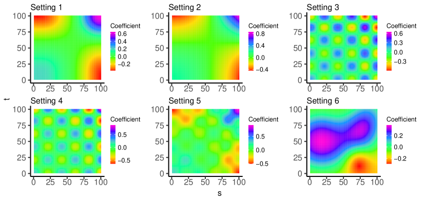
Figure 1: Heat-map plots of the true coefficient functions $\beta_{0}(s,t)$ in Model (3).

Specifically, for the first four settings, the coefficient functions are given by

$$\alpha_{0}(t)=\beta_{0}(t)=4\sqrt{2}\sum_{i=1}^{n_{\textrm{eig}}}(-1)^{i}i^{-2}\cos\big{(}(i+k_{\textrm{mis}})\pi t\big{)}.$$ (16)

Here, $n_{\textrm{eig}}$ controls the number of eigenfunctions in the coefficient function and will be set to be 4 and 200 later. Furthermore, $k_{\textrm{mis}}$ controls the degree of misalignment between the covariance eigen structure in (15) and the leading basis functions in the coefficient function (16). Because the leading eigenfunctions in (15) are ordered from the first to the last as $i=1,2,\ldots,200$ in $\cos(i\pi t)$, while the first leading basis function in (16) is $\cos\big{(}(1+k_{\textrm{mis}})\pi t\big{)}$. When $k_{\textrm{mis}}=0$, there is no misalignment. As $k_{\textrm{mis}}$ increases, the misalignment becomes more severe. Settings 1-4 consider combinations of $n_{\textrm{eig}}\in\{4,200\}$ and $k_{\textrm{mis}}\in\{0,4\}$, with detailed configurations in Table 1.

Setting	$n_{\textrm{eig}}$	$k_{\textrm{mis}}$	indices $i$ of basis function $\cos(i\pi t)$	indices $i$ of basis function $\cos(i\pi t)$
			in the covariances $C_{\alpha}$ and $C_{\beta}$	in the coefficient $\alpha_{0}(\cdot),\beta_{0}(\cdot)$
1	4	0	$1,2,\ldots,200$	$1,2,3,4$
2	200	0	$1,2,\ldots,200$	$1,2,\ldots,200$
3	4	4	$1,2,\ldots,200$	$5,6,7,8$
4	200	4	$1,2,\ldots,200$	$5,6,\ldots,204$

Table 1: The configurations of the covariances and coefficient functions for Settings 1-4.

Settings 5-6 are based on Model (3), where the true coefficient function $\beta_{0}(s,t)$ is indeed two-dimensional, instead of the product of two 1D functions as our model assumes. Setting 5 considers a two-dimensional coefficient function, as the sum of two terms, where each term is a product of two 1D functions, $\beta_{0}(s,t)=\alpha_{0}^{[1]}(s)\beta_{0}^{[1]}(t)+0.4\alpha_{0}^{[2]}(s)\beta_{0}^{[2]}(t)$, where $\alpha_{0}^{[1]}(t)=\beta_{0}^{[1]}(t)=4\sqrt{2}\sum_{i=1}^{4}(-1)^{i}i^{-2}\cos(i\pi t)$, $\alpha_{0}^{[2]}(t)=\beta_{0}^{[2]}(t)=4\sqrt{2}\sum_{i=1}^{4}(-1)^{i}i^{-2}\cos\big{(}(i+4)\pi t\big{)}$.

Setting 6 uses a two-dimensional coefficient function borrowed from the GMRF literature (Happ et al., 2018). We magnified their coefficient function by four times to make its Frobenius norm maintain at the same level as those of the other five settings.

Under these six settings, the data are generated according to Model (2) or (3), where $\mu_{0}=0$, and noise level $\sigma=0.5$. The predictor $X(s,t)$ follows a centered Gaussian process with the covariance structure described above. The sample size $n=2^{5}$, $2^{6}$, $2^{7}$, and $2^{8}$. The continuous functions are observed on a regular grid of length 100. For each value of $r_{c}$ and each value of $n$, we repeat the experiments 100 times. The numerical results for different level of smoothness are similar. Hence, to save space, we present the results for all four choices of $r_{c}$ for Setting 1, and only for $r_{c}=1$ for the other five settings. The associated kernel function for the RKHS of FBLR is the same,

$$K(s,t)=-B_{4}(|s-t|/2)/3-B_{4}((s+t)/2)/3,$$ (17)

where $B_{4}(\cdot)$ is the 4th Bernoulli polynomial. This kernel function corresponds to the Hilbert norm $\parallel f\parallel^{2}_{\mathcal{H}}=\int(f^{\prime\prime})^{2}$.

4.2 Simulation results

Under Setting 1, we first examine the performance of FBLR. As discussed in Section 2.4, the implementation of our method needs special attention to the covariance structure estimation, tuning parameter selection, and proper initialization. We include both the true covariances $C_{\alpha},C_{\beta}$ and the estimated ones $\hat{C_{\alpha}},\hat{C_{\beta}}$, with the truth as the oracle benchmark. We also consider two choices of tuning parameter selections, CV and iGCV. These choices lead to FBLR+CV+true, FBLR+iGCV+true, FBLR+CV+est, and FBLR+iGCV+est. We further compare three choices of initialization methods: Ridge after vectorization, PFPCR and MFPCR, which lead to multiple versions of our methods: Ridge$\to$FBLR, PFPCR$\to$FBLR and MFPCR$\to$FBLR, correspondingly.

Figure 2 shows the results of excess risk when considering tuning parameter selection via CV vs. iGCV. Each panel demonstrates a linear relationship between log(risk) and $\log(n)$, and further reveals that the larger the $r_{c}$, the faster the convergence. These reconfirm the convergence rate developed theoretically in Theorem 2, where $r=r_{c}+1$. The four panels are almost identical, implying that the computationally-inexpensive iGCV performs similar as the computationally-expensive CV, and FBLR with the estimated covariances performs as well as with the true covariances. Hereafter, FBLR means FBLR+iGCV+est for these reasons. Since multiple $r_{c}$’s show similar messages, we will only use $r_{c}=1$ from now on.

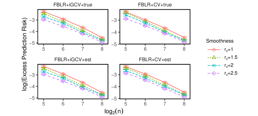
Figure 2: Plots of the excess prediction risk vs. the sample size $n$ with both axes in log scale under Setting 1. Four sample sizes and four values of $r_{c}$ are considered. The error bars are generated according to mean $\pm$ one SE. The four panels are all for FBLR approaches, including FBLR+iGCV+true, FBLR+CV+true, FBLR+iGCV+est, and FBLR+CV+est.

Figure 3 shows the performance of FBLR with three different initialization methods under Setting 1 with $r_{c}=1$. Initializing via Ridge, PFPCR or MFPCR produces indistinguishable results from the perspective of prediction risk. As for the computational time, it can be seen most of the time is spent on initialization, and FBLR itself takes little time to implement. Because of these observations and the fastest computation of Ridge, for the rest of this article, we will use Ridge as initialization, together with FBLR+iGCV+est.

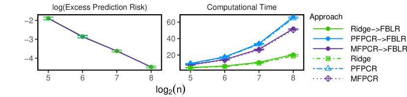
Figure 3: Plots of the logarithm of excess prediction risk and computation time vs. the sample size $n$ in log scale with $r_{c}=1$ under Setting 1. The error bars are mean $\pm$ one SE.

For Settings 1-4, Figure 4 compares FBLR and a few other existing methods, such as PFPCR, MFPCR, and GMRF, in terms of the prediction risk and computation time. In the implementation of PFPCR and MFPCR, one needs to specify the maximum number $r^{\max}$ of PCs, and the package will automatically find the optimal number of PCs. According to Table 1, the theoretically optimal numbers of PCs to be provided to estimate the coefficient functions in the noiseless case are 4, 200, 8, and 204, for Settings 1-4 respectively. We tried two choices of $r^{\max}\in\{4,8\}$. Additionally, in Appendix E of the Supplement, we examine the choice of $r^{\textrm{max}}=\lfloor\sqrt{n-1}\rfloor$, which means we provide the code with the largest possible number of PCs that the software can handle. A brief message is that $r^{\max}=\lfloor\sqrt{n-1}\rfloor$ is extremely time-consuming and even less accurate than the other two. So for this section, only $r^{\max}\in\{4,8\}$ are compared with FBLR.

In Figure 4, it is not surprising to see that GMRF is not doing well statistically under all settings, albeit its fastest speed, because it does not take advantage of the low-rank structure of the coefficient function. This figure also shows that the statistical performance of the prediction risk of FBLR dominates all other methods under all four Settings 1-4. From the perspective of computational cost, FBLR is always much faster than 2D-FPCR with $r^{\textrm{max}}=8$, faster than 2D-FPCR with $r^{\textrm{max}}=4$ under Settings 1-2 and when the sample size is large under Settings 3-4.

Under Setting 1, even though ${\rm PFPCR}_{r_{\max}=4}$ and ${\rm MFPCR}_{r_{\max}=4}$ have the oracle knowledge of the true number of PCs and are perfectly aligned with the coefficient function, they are still worse than the penalized approach FBLR. Under Setting 1, ${\rm PFPCR}_{r_{\max}=8}$ and ${\rm MFPCR}_{r_{\max}=8}$ are worse than ${\rm PFPCR}_{r_{\max}=4}$ and ${\rm MFPCR}_{r_{\max}=4}$, because some unnecessary and noisy PCs are estimated. Under Setting 2, although more basis functions, 200 in total to be exact, are involved in the coefficient functions, $r^{\textrm{max}}=4$ still out-performs $r^{\textrm{max}}=8$ when $\log_{2}(n)=7$ because of smaller variance given the small sample size; $r^{\textrm{max}}=8$ and $r^{\textrm{max}}=4$ are comparable when the sample size reaches $\log_{2}(n)=8$.

Under Settings 3-4, there is misalignment, and so 2D-FPCR with $r^{\textrm{max}}=4$ is completely off (the leading four PCs are orthogonal to the true coefficient functions). Therefore, $r^{\textrm{max}}=8$ performs better than $r^{\textrm{max}}=4$. But $r^{\textrm{max}}=8$ is still not as accurate as FBLR. In summary, when the true model is indeed bilinear (2) under Settings 1-4, no matter misalignment exists or not, the penalized approach is more robust to the alignment structure than the PC-based approach, produces better prediction, and has less computational burden.

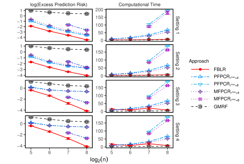
Figure 4: Plots of the logarithm of the excess prediction risk and computation time vs. the sample size $n$ in log scale for Settings 1-4 with $r_{c}=1$. The error bars are generated according to mean $\pm$ one SE. ${\rm PFPCR}_{r_{\max}=8}$ and ${\rm MFPCR}_{r_{\max}=8}$ are only shown for $\log_{2}(n)=7,8$, because they require larger sample size.

For Settings 5-6, Figure 5 compares the performance of prediction risk and computational time. Settings 5 and 6 follow Model (4) and Model (3) respectively, both of which violate the model assumption (2), and therefore puts the FBLR in a disadvantageous situation. We used the iterative idea, discussed after Model (4), to apply FBLR twice: once on the original data $y_{i}$ and once on the residual $e_{i}$. We denote this approach as ${\rm FBLR}_{R=2}$, and obtain the estimate of the two-dimensional coefficient function of the form $\hat{\beta}_{0}(s,t)=\sum_{r=1}^{2}\hat{\alpha}_{0}^{[r]}(s)\hat{\beta}_{0}^{[r]}(t)$.

Under Setting 5, ${\rm FBLR}_{R=2}$ is always statistically better than PFPCR, MFPCR, and GMRF and computationally faster than PFPCR and MFPCR. Even though the true model consists of two terms, when the sample size is small, estimating one term by FBLR is the best. When the sample size becomes larger, estimating two terms by ${\rm FBLR}_{R=2}$ pays off. Under Setting 6, ${\rm FBLR}_{R=2}$ performs the best, followed by ${\rm PFPCR}_{r^{\textrm{max}}=4}$ and ${\rm MFPCR}_{r^{\textrm{max}}=4}$, and FBLR is worse. In summary, if the bilinear model (2) does not hold while Models (3)-(4) do, one can resort to iterative-FBLR to estimate multiple terms.

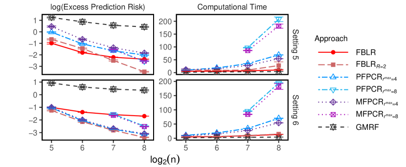
Figure 5: Same as Figure 4, but for Settings 5-6.

5 Real data analysis: Canadian weather

We perform real data analysis on two datasets, the Canadian weather data in this section and the LIDAR data in Appendix G.

The Canadian weather data has been widely used for FDA. Traditionally, it is typically used for 1D-FPCA, 1D-FPCR (Ramsay and Silverman, 2005b) or 1D-FLR (Cai and Yuan, 2012), where each vector is of length 365, containing the daily temperature averaged over 24 hours and averaged over a few years. We consider the matrices $x_{i}\in\mathbb{R}^{365\times 24}$, where $x_{i}(s,t)$ is the temperature in the $t$-th hour of the $s$-th day of the year averaged over 2002-2021. Hence, it contains extra hourly information compared to 1D analysis. Following Ramsay and Silverman (2005b); Cai and Yuan (2012), the response variable $y_{i}$ is the logarithm of the average annual precipitation over 2002-2021, and 35 weather stations are included.

We compare the performances of FBLR and some existing methods, including PFPCR, MFPCR, GMRF, Ridge after vectorization, and two variants of 1D-FLR. The first variant is to adopt the FLR method in Cai and Yuan (2012) after matrix vectorization, denoted by FLR+vec. (See Appendix E for further discussion on the potential twist of the vectorization approach.) The second variant is to apply FLR on the vectors of length 365, which are obtained by averaging temperatures over 24 hours, $\sum_{t=1}^{24}x_{i}(s,t)/24$, denoted by FLR+ave. Both FBLR and FLR-related methods choose the kernel $K_{1}(s,t)=K_{2}(s,t)=1-B_{4}(|s-t|)/24$, which is used in Cai and Yuan (2012) as well. For PFPCR and MFPCR, we use $r^{\textrm{max}}=\lfloor\sqrt{n-1}\rfloor=5$. BLR (FBLR with no penalty) was not compared because the sample size is not large enough to estimate the parameters.

We first compare all methods from the perspective of prediction accuracy and computational time in Figure 6. The leave-one-out method is used to calculate the out-of-sample squared error. FBLR works the best compared to the other 2D and 1D methods, and the differences are all significant because the p-value of the paired t-test between FBLR and each of the other methods is less than 0.05. GMRF performs the worst. MFPCR is similar to and PFPCR is worse than all three 1D methods including Ridge, FLR+vec, and FLR+ave. Furthermore, FLR+ave, the traditional 1D FDA method by Cai and Yuan (2012), performs worse than FBLR, suggesting that the temperature variations along the hour-of-the-day dimension contain extra information for predicting annual precipitation. As for the computational time, it is unsurprising to see that FBLR takes longer time than Ridge and FLR+ave, because FBLR uses Ridge as initialization, and FLR+ave has a 1D predictor of length 365 instead of a 2D predictor of size 365 $\times$ 24.

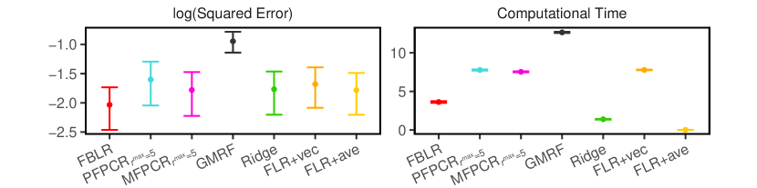
Figure 6: Plots of the out-of-sample performance on the Canadian weather data, which include the testing error and computational time. The error bars are mean $\pm$ one SE.

Figure 7 displays the heat-maps of the estimated 2D coefficient function $\hat{\beta}(s,t)$ in Model (3) for all approaches. For FLR+ave, the 2D function is generated from their estimated 1D coefficient function $\hat{\beta}(\cdot)$ in Model (1) by repeating the yearly pattern for each hour, i.e., $\hat{\beta}(s,t)=\hat{\beta}(s)\times\frac{1}{24}$ for $s=1,\ldots,365$ and $t=1,\ldots,24$.

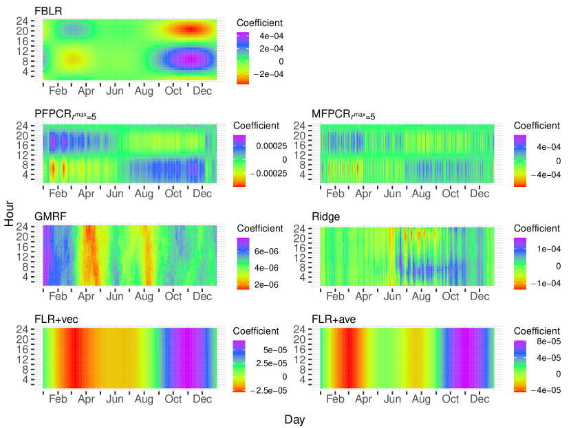
Figure 7: Plots of the estimated 2D coefficient function $\hat{\beta}(s,t)$ in Model (3) by seven methods for Canadian weather data. The $x$ and $y$ axes correspond to day and hour respectively.

As the figure shows, FBLR produces a smoother coefficient function estimation compared with the other 2D methods. Furthermore, despite PFPCR and MFPCR being designed to generate smooth estimations, the actual estimated coefficient functions are not as smooth as expected, especially for the time-of-the-day dimension. For the 1D methods, Ridge estimation is non-smooth, and both FLR+vec and FLR+ave are over-smoothed since the hour dimension has almost no variation.

Figure 8 provides the visualization of the estimated coefficient functions $\hat{\alpha}(\cdot)$ and $\hat{\beta}(\cdot)$ in Model (2). For those methods that do not estimate the 1D coefficient functions directly, the leading left and right singular vectors of the estimated 2D coefficient functions are plotted.

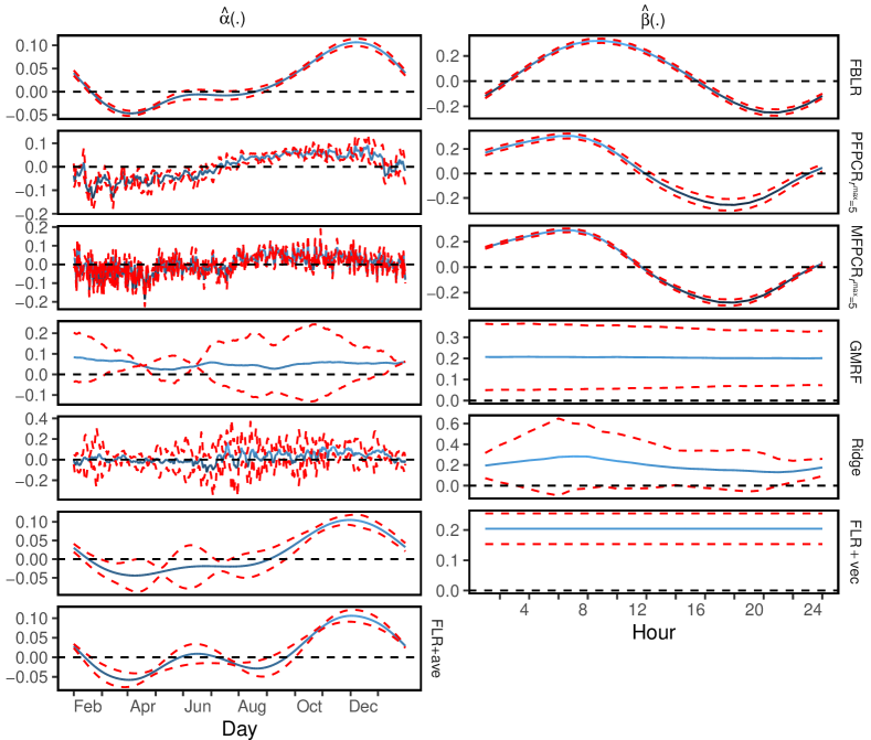
Figure 8: Plots of the estimated 1D coefficient functions $\hat{\alpha}(\cdot)$ and $\hat{\beta}(\cdot)$ in Model (2) by seven methods for Canadian weather data. The confidence intervals correspond to 95% confidence level.

From the left panels for the day-of-the-year effect, it can be seen that PFPCR, MFPCR, and Ridge are not smooth, GMRF is not quite significant, the bandwidth of FLR+vec is wide, and FBLR and FLR+ave (Cai and Yuan, 2012) are rather similar with a peak near November and a trough near March. Such a contrast between Spring and Fall appears at moisture-laden coastal locations (Donohoe et al., 2020), which have warmer autumns and cooler springs than inland stations. As a consequence, they have more precipitation. However, there is slight difference between FBLR and FLR+ave in that the confidence intervals throughout Summer contain zero for FBLR but not for FLR+ave, which implies that temperature variation in the summer has no effect on the precipitation from the results of FBLR. This makes sense, as the temperature in the summer at coastal and inland stations has no strong correlation with maritime effect.

From the right panels for the time-of-the-day effect, it can be seen that GMRF, Ridge, and FLR+vec estimations essentially suggest that there is no hourly effect, while FBLR, PFPCR, and MFPCR reveal and share a significant effect. The estimated $\hat{\beta}(\cdot)$’s by the latter three say that more precipitation occurs with warmer daytime and cooler nighttime. In other words, more precipitation accompanies larger diurnal temperature variation, which promotes the local breeze circulations caused by land-water temperature differences (e.g., Yang and Smith, 2006), and is essential to convective precipitation in the areas near water bodies (e.g. sea, gulf, lake and river). The residuals of FBLR are examined in Appendix F, which suggests a fairly good fit of the data.

6 Discussion

This article studies the problem of regression of a scalar response on a two-dimensional functional predictor, which when observed on 2D grid becomes a matrix predictor. We propose a functional regression model where the two-dimensional coefficient function is assumed to adopt the form of a product of two 1D coefficient functions. We offer an iterative strategy for the circumstance when the two-dimensional coefficient function can be well approximated by the sum of a few products, which implies low rank for matrix coefficient matrix. We estimate the model via an innovative penalized approach and compare the penalized approach with the approach of regression on two-dimensional PCs and other methods. We show that the misalignment issue of the PC regression remains as in the 1D FLR case. Even if misalignment does not occur, the penalized approach still performs better than the PCR approach because of further shrinkage. Moreover, the penalized approach also exhibits a huge computational advantage. Real data application further demonstrates the “stableness” and smoothness of the penalized approach.

There are a few meaningful directions for future extensions. The first is to rigorously understand Model (4) with multiple terms, such as how to determine the optimal $R$. Empirically, one can choose this tuning parameter via cross-validation or similar approaches. Theoretically, this is a challenging topic worth studying further. The second one is to extend from scalar-on-matrix functional regression to scalar-on-tensor functional regression, under which case, a careful design of the penalty function is necessary. The LIDAR task in Appendix G intrinsically requires such an extension to consider time, spatial range, and wavelength as a three-dimensional predictor. The third one is to extend from a linear model to a generalized linear model for classification and other purposes. For example, one may want to classify whether a person has Alzheimer’s disease based on the fMRI data, which has spatial and temporal smooth input.

Supplementary materials

The materials include proofs of main theorems and all lemmas, additional discussions on the penalty function, additional simulation results, additional results of the real data analysis of the Canadian weather, and the second real data example of the LIDAR data.

In this supplement, we provide proofs of the main theorems in Section A, all lemmas and their detailed proofs in Sections B-C. We also present more discussion on the penalty in Section D additional simulation result in Section E, additional real data analysis on the Canadian weather in Section F, and the real data example of LIDAR data in Section G.

Appendix A Proofs of main theorems

A.1 Proof of Theorem 2

In this section, we will show the proof of Theorem 2. We start by providing a result from Yuan and Cai (2010) that will be extensively used in the proof.

Lemma 5 (Theorem 3 of Yuan and Cai (2010))

For any function $f\in\mathcal{H}(K)$, it can be written as $f=\sum_{k=1}^{\infty}f_{k}\omega_{k}$, where $f_{k}=s_{k}^{T}\langle f,\omega_{k}\rangle_{R}$. Moreover, the quadratic forms $\|\cdot\|_{R}^{2}$, $\|\cdot\|_{K}^{2}$, and $\|\cdot\|_{0}^{2}$ can be expressed as $\|f\|_{R}^{2}=\sum_{k=1}^{\infty}(1+\gamma_{k}^{-1})f_{k}^{2}$, $\|f\|_{0}^{2}=\sum_{k=1}^{\infty}f_{k}^{2}$, and $\|f\|_{K}^{2}=\sum_{k=1}^{\infty}\gamma_{k}^{-1}f_{k}^{2}$.

Lemma 5 demonstrates that the norms $\|\cdot\|_{R}^{2}$, $\|\cdot\|_{K}^{2}$, and $\|\cdot\|_{0}^{2}$ can be expressed on the basis $\omega_{k},k=1,2,...$, which was defined in Section 3.1. See Yuan and Cai (2010) for the elementary proof of Lemma 5.

Recall the definition of the excess prediction risk, from the identity, $\widehat{\alpha}(s)\widehat{\beta}(t)-\alpha_{0}(s)\beta_{0}(t)=\\ \big{(}\widehat{\alpha}(s)-\alpha_{0}(s)\big{)}\big{(}\widehat{\beta}(t)-\beta_{0}(t)\big{)}+\big{(}\widehat{\alpha}(s)-\alpha_{0}(s)\big{)}\beta_{0}(t)+\big{(}\widehat{\beta}(t)-\beta_{0}(t)\big{)}\alpha_{0}(s)$, and the definition of $\|\cdot\|_{0}$ norm as in (5) and the property (6), it follows that the excess prediction risk can be further bounded by three terms,

$$\mathcal{E}(\widehat{\alpha},\widehat{\beta};\alpha_{0},\beta_{0})\leq 3\|\widehat{\alpha}-\alpha_{0}\|_{0}^{2}\|\widehat{\beta}-\beta_{0}\|_{0}^{2}+3\|\widehat{\alpha}-\alpha_{0}\|_{0}^{2}\|\beta_{0}\|_{0}^{2}+3\|\alpha_{0}\|_{0}^{2}\|\widehat{\beta}-\beta_{0}\|_{0}^{2}.$$ (18)

Therefore, we only need to bound two terms $\|\widehat{\alpha}-\alpha_{0}\|_{0}^{2}$ and $\|\widehat{\beta}-\beta_{0}\|_{0}^{2}$. Due to symmetry in $\alpha$ and $\beta$, one bound on $\|\widehat{\alpha}-\alpha_{0}\|_{0}^{2}$ is sufficient for the problem. However, in what follows, we shall bound $\|\widehat{\alpha}-\alpha_{0}\|_{a}^{2}$ due to the necessity in the proof, where the norm $\|\cdot\|_{a}$ for $0\leq a\leq 1$ is defined by $\|f\|_{a}^{2}=\sum_{k=1}^{\infty}(1+\gamma_{k}^{-a})f_{k}^{2},$ when $f=\sum_{k=1}^{\infty}f_{k}\omega_{k}$. Clearly, $\|\cdot\|_{a}$ reduces to $\|\cdot\|_{0}$ by a factor of 2 when $a=0$ due to Lemma 5.

Recall that the objective function for the optimization problem is $\ell_{n\lambda}(\alpha,\beta)=\ell_{n}(\alpha,\beta)+J(\alpha,\beta)$, and the smoothness regularized estimator is obtained via $(\widehat{\alpha},\widehat{\beta})=\arg\min\ell_{n\lambda}(\alpha,\beta).$ Write $\ell(\alpha,\beta)=\mathbb{E}\ell_{n}(\alpha,\beta)$, and $\ell_{\lambda}(\alpha,\beta)=\mathbb{E}\ell_{n\lambda}(\alpha,\beta)$, to be the expectations of $\ell_{n}(\alpha,\beta)$ and $\ell_{n\lambda}(\alpha,\beta)$ respectively. The convention is to use subscript $n$ to denote the sample version and without subscript for the population counterpart. Denote the minimizer of $\ell_{\lambda}(\alpha,\beta)$ by $(\bar{\alpha},\bar{\beta})$, that is, $(\bar{\alpha},\bar{\beta})=\arg\min\ell_{\lambda}(\alpha,\beta)=\arg\min\ell(\alpha,\beta)+J(\alpha,\beta)$. To bound $\|\widehat{\alpha}-\alpha_{0}\|_{a}$, one can bound $\|\bar{\alpha}-\alpha_{0}\|_{a}$ and $\|\widehat{\alpha}-\bar{\alpha}\|_{a}$, which can be thought of as the deterministic error (or bias) and stochastic error (or variance) respectively.

To bound the stochastic error term, another pair $(\tilde{\alpha},\tilde{\beta})$ has to be introduced so that $\|\widehat{\alpha}-\bar{\alpha}\|_{a}\leq\|\widehat{\alpha}-\tilde{\alpha}\|_{a}+\|\tilde{\alpha}-\bar{\alpha}\|_{a}$. Here $(\tilde{\alpha},\tilde{\beta})$ can be thought of as the expansion and is defined by

$$\left(\begin{array}[]{c}\tilde{\alpha}\\ \tilde{\beta}\end{array}\right)=\left(\begin{array}[]{c}\bar{\alpha}\\ \bar{\beta}\end{array}\right)-H^{-1}\left(\begin{array}[]{c}D_{\alpha}\ell_{n\lambda}(\bar{\alpha},\bar{\beta})\\ D_{\beta}\ell_{n\lambda}(\bar{\alpha},\bar{\beta})\end{array}\right),$$ (19)

where

$$H=\left(\begin{array}[]{cc}D^{2}_{\alpha\alpha}\ell_{\lambda}(\bar{\alpha},\bar{\beta})&D^{2}_{\alpha\beta}\ell_{\lambda}(\bar{\alpha},\bar{\beta})\\ D^{2}_{\beta\alpha}\ell_{\lambda}(\bar{\alpha},\bar{\beta})&D^{2}_{\beta\beta}\ell_{\lambda}(\bar{\alpha},\bar{\beta})\\ \end{array}\right),$$ (20)

where the following operators are defined. The first set of operators are the first- and second-order derivatives of the sample and population loss functions $\ell_{n}$ and $\ell$,

$$D_{\alpha}\ell_{n}(\alpha,\beta)f = -\frac{2}{n}\sum_{i=1}^{n}\left(y_{i}-\int_{\mathcal{T}\times\mathcal{T}}x_{i}(s,t)\alpha(s)\beta(t)~{}dsdt\right)\left(\int_{\mathcal{T}\times\mathcal{T}}x_{i}(s,t)f(s)\beta(t)~{}dsdt\right),$$

$$D_{\beta}\ell_{n}(\alpha,\beta)f = -\frac{2}{n}\sum_{i=1}^{n}\left(y_{i}-\int_{\mathcal{T}\times\mathcal{T}}x_{i}(s,t)\alpha(s)\beta(t)~{}dsdt\right)\left(\int_{\mathcal{T}\times\mathcal{T}}x_{i}(s,t)\alpha(s)f(t)~{}dsdt\right),$$

$$D^{2}_{\alpha\alpha}\ell_{n}(\alpha,\beta)fg = \frac{2}{n}\sum_{i=1}^{n}\left(\int_{\mathcal{T}\times\mathcal{T}}x_{i}(s,t)f(s)\beta(t)~{}dsdt\right)\left(\int_{\mathcal{T}\times\mathcal{T}}x_{i}(s,t)g(s)\beta(t)~{}dsdt\right),$$

$$D^{2}_{\beta\beta}\ell_{n}(\alpha,\beta)fg = \frac{2}{n}\sum_{i=1}^{n}\left(\int_{\mathcal{T}\times\mathcal{T}}x_{i}(s,t)\alpha(s)f(t)~{}dsdt\right)\left(\int_{\mathcal{T}\times\mathcal{T}}x_{i}(s,t)\alpha(s)g(t)~{}dsdt\right),$$

$$D^{2}_{\alpha\beta}\ell_{n}(\alpha,\beta)fg = -\frac{2}{n}\sum_{i=1}^{n}\left(y_{i}-\int_{\mathcal{T}\times\mathcal{T}}x_{i}(s,t)\alpha(s)\beta(t)~{}dsdt\right)\left(\int_{\mathcal{T}\times\mathcal{T}}x_{i}(s,t)f(s)g(t)~{}dsdt\right)$$

$$+\frac{2}{n}\sum_{i=1}^{n}\left(\int_{\mathcal{T}\times\mathcal{T}}x_{i}(s,t)f(s)\beta(t)~{}dsdt\right)\left(\int_{\mathcal{T}\times\mathcal{T}}x_{i}(s,t)\alpha(s)g(t)~{}dsdt\right),$$

$$D_{\alpha}\ell(\alpha,\beta)f = -2\int_{\mathcal{T}^{4}}C(s_{1},s_{2})C(t_{1},t_{2})\big{(}\alpha_{0}(s_{1})\beta_{0}(t_{1})-\alpha(s_{1})\beta(t_{1})\big{)}f(s_{2})\beta(t_{2})~{}ds_{1}ds_{2}dt_{1}dt_{2},$$

$$D_{\beta}\ell(\alpha,\beta)f = -2\int_{\mathcal{T}^{4}}C(s_{1},s_{2})C(t_{1},t_{2})\big{(}\alpha_{0}(s_{1})\beta_{0}(t_{1})-\alpha(s_{1})\beta(t_{1})\big{)}\alpha(s_{2})f(t_{2})~{}ds_{1}ds_{2}dt_{1}dt_{2},$$

$$D^{2}_{\alpha\alpha}\ell(\alpha,\beta)fg = 2\|\beta\|_{0}^{2}\int_{\mathcal{T}\times\mathcal{T}}C(s,t)f(s)g(t)~{}dsdt,$$

$$D^{2}_{\beta\beta}\ell(\alpha,\beta)fg = 2\|\alpha\|_{0}^{2}\int_{\mathcal{T}\times\mathcal{T}}C(s,t)f(s)g(t)~{}dsdt,$$

$$D^{2}_{\alpha\beta}\ell(\alpha,\beta)fg = -2\left(\int_{\mathcal{T}\times\mathcal{T}}C(s,t)\alpha_{0}(s)f(t)dsdt\right)\left(\int_{\mathcal{T}\times\mathcal{T}}C(s,t)\beta_{0}(s)g(t)dsdt\right)$$

$$+4\left(\int_{\mathcal{T}\times\mathcal{T}}C(s,t)\alpha(s)f(t)dsdt\right)\left(\int_{\mathcal{T}\times\mathcal{T}}C(s,t)\beta(s)g(t)dsdt\right),$$

and the second set of operators are first- and second-order derivatives of the sample and population objective functions $\ell_{n\lambda}$ and $\ell_{\lambda}$,

$$D_{\alpha}\ell_{n\lambda}(\alpha,\beta) = D_{\alpha}\ell_{n}(\alpha,\beta)+D_{\alpha}J(\alpha,\beta),$$

$$D_{\beta}\ell_{n\lambda}(\alpha,\beta) = D_{\beta}\ell_{n}(\alpha,\beta)+D_{\beta}J(\alpha,\beta),$$

$$D^{2}_{\alpha\alpha}\ell_{n\lambda}(\alpha,\beta) = D^{2}_{\alpha\alpha}\ell_{n}(\alpha,\beta)+D^{2}_{\alpha\alpha}J(\alpha,\beta),$$

$$D^{2}_{\beta\beta}\ell_{n\lambda}(\alpha,\beta) = D^{2}_{\beta\beta}\ell_{n}(\alpha,\beta)+D^{2}_{\beta\beta}J(\alpha,\beta),$$

$$D^{2}_{\alpha\beta}\ell_{n\lambda}(\alpha,\beta) = D^{2}_{\alpha\beta}\ell_{n}(\alpha,\beta)+D^{2}_{\alpha\beta}J(\alpha,\beta),$$

$$D_{\alpha}\ell_{\lambda}(\alpha,\beta) = D_{\alpha}\ell(\alpha,\beta)+D_{\alpha}J(\alpha,\beta),$$

$$D_{\beta}\ell_{\lambda}(\alpha,\beta) = D_{\beta}\ell(\alpha,\beta)+D_{\beta}J(\alpha,\beta),$$

$$D^{2}_{\alpha\alpha}\ell_{\lambda}(\alpha,\beta) = D^{2}_{\alpha\alpha}\ell(\alpha,\beta)+D^{2}_{\alpha\alpha}J(\alpha,\beta),$$

$$D^{2}_{\beta\beta}\ell_{\lambda}(\alpha,\beta) = D^{2}_{\beta\beta}\ell(\alpha,\beta)+D^{2}_{\beta\beta}J(\alpha,\beta),$$

$$D^{2}_{\alpha\beta}\ell_{\lambda}(\alpha,\beta) = D^{2}_{\alpha\beta}\ell(\alpha,\beta)+D^{2}_{\alpha\beta}J(\alpha,\beta).$$

By the triangle inequality, we have

$$\|\widehat{\alpha}-\alpha_{0}\|_{a}=\|(\widehat{\alpha}-\tilde{\alpha})+(\tilde{\alpha}-\bar{\alpha})+(\bar{\alpha}-\alpha_{0})\|_{a}\leq\|\widehat{\alpha}-\tilde{\alpha}\|_{a}+\|\tilde{\alpha}-\bar{\alpha}\|_{a}+\|\bar{\alpha}-\alpha_{0}\|_{a}.$$ (21)

Lemmas 6, 7 and 8 in Section B establish bounds for the three terms on the right hand side of (21) respectively and together with (21) imply that, if $\lambda=O(n^{-2r/(2r+1)})$,

$$\lim_{A\rightarrow\infty}\lim_{n\rightarrow\infty}\sup_{\begin{subarray}{c}\alpha_{0}\in\mathcal{H}(K),\\ \beta_{0}\in\mathcal{H}(K)\end{subarray}}\mathbb{P}(\|\widehat{\alpha}-\alpha_{0}\|_{0}^{2}\geq An^{-\frac{2r}{2r+1}}) = 0,$$ (22)

$$\lim_{A\rightarrow\infty}\lim_{n\rightarrow\infty}\sup_{\begin{subarray}{c}\alpha_{0}\in\mathcal{H}(K),\\ \beta_{0}\in\mathcal{H}(K)\end{subarray}}\mathbb{P}(\|\widehat{\beta}-\beta_{0}\|_{0}^{2}\geq An^{-\frac{2r}{2r+1}}) = 0.$$ (23)

Combining (22), (23) and (18) completes the proof of Theorem 2. $\blacksquare$

Comment: Note that the proof to 2D FBLR differs much from the proof to 1D FLR since FLR only requires expansion of $\tilde{\beta}$ whereas FBLR relies on 2D expansion (19) which complicates the proofs of the lemmas extensively. To save the readers some detour, expanding $\tilde{\alpha},\tilde{\beta}$ separately without considering their interaction cannot lead to the full proof.

A.2 Proof of Theorem 4

Note that although it has been assumed throughout that the noise $\epsilon$ has mean zero and finite variance, for the proof of lower bound, it suffices to assume the normal case $\epsilon\sim N(0,\sigma^{2})$. This is because any lower bound for the normal case yields a lower bound for the general case without normality.

We will invoke Lemma 15 in Section C.1 from Tsybakov (2009). To that end, we construct a parameter space $\Theta$ that contains elements $\theta=(\theta_{N+1},...,\theta_{2N})^{T}\in\{0,1\}^{N}$, where $N$ is the smallest integer such that $N\geq c_{1}n^{1/(2r+1)}$ for some constant $c_{1}>0$ whose value will be specified later. The slope function $\alpha$ depends on $\theta$ through

$$\alpha_{\theta}=N^{-1/2}\sum_{k=N+1}^{2N}\theta_{k}\gamma_{k}^{1/2}\omega_{k}.$$ (24)

Then it is easy to verify that

$$\|\alpha_{\theta}\|_{K}^{2}=N^{-1}\sum_{k=N+1}^{2N}\theta_{k}^{2}\gamma_{k}\|\omega_{k}\|_{K}^{2}=N^{-1}\sum_{k=N+1}^{2N}\theta_{k}^{2}\leq N^{-1}\sum_{k=N+1}^{2N}1=1,$$

which proves that $\alpha_{\theta}\in\mathcal{H}$.

Define the parameter space $\Theta$ as $\Theta=\{\theta^{(0)},\theta^{(1)},...,\theta^{(M)}\}\subset\{0,1\}^{N}$. For $N\geq 8$, Gilbert Shannon Varshamov bound guarantees that the following conditions hold simultaneously:

1. $\theta^{(0)}=(0,...,0)^{T}$,

2. $H(\theta,\theta^{\prime})>N/8$ for any pair $\theta\neq\theta^{\prime}\in\Theta$, where $H$ is the Hamming distance,

3. The cardinality of the set is at least $M\geq 2^{N/8}$.

Denote by $P_{\theta}$ the joint distribution of $(X_{i},Y_{i}),i=1,...,n$ given $\alpha_{0}=\alpha_{\theta},\beta_{0}=\omega_{1}$, then the ratio of the density becomes

$$\log\frac{P_{\theta}}{P_{\theta^{\prime}}}=\frac{2\sum_{i=1}^{n}\left(Y_{i}-\int X_{i}\alpha_{\theta}\omega_{1}\right)\int X_{i}(\alpha_{\theta}\omega_{1}-\alpha_{\theta^{\prime}}\omega_{1})+\sum_{i=1}^{n}\left(\int X_{i}(\alpha_{\theta}\omega_{1}-\alpha_{\theta^{\prime}}\omega_{1})\right)^{2}}{2\sigma^{2}}.$$ (25)

Based on this expression, the Kullback-Leibler distance between $P_{\theta}$ and $P_{\theta^{\prime}}$ can be computed $KL(P_{\theta},P_{\theta^{\prime}})=\int\log\frac{P_{\theta}}{P_{\theta^{\prime}}}P_{\theta}=\frac{n}{2\sigma^{2}}\|\alpha_{\theta}-\alpha_{\theta^{\prime}}\|_{0}^{2}\|\omega_{1}\|_{0}^{2}$. Plugging in $\alpha_{\theta}$ (24) leads to

$$KL(P_{\theta},P_{\theta^{\prime}}) = \frac{n}{2\sigma^{2}}\left\|N^{-1/2}\sum_{k=N+1}^{2N}(\theta_{k}-\theta^{\prime}_{k})\gamma_{k}^{1/2}\omega_{k}\right\|_{0}^{2}=\frac{n}{2N\sigma^{2}}\sum_{k=N+1}^{2N}(\theta_{k}-\theta^{\prime}_{k})^{2}\gamma_{k}$$

$$\leq \frac{n\gamma_{N}}{2N\sigma^{2}}\sum_{k=N+1}^{2N}(\theta_{k}-\theta^{\prime}_{k})^{2}\leq\frac{n\gamma_{N}}{2N\sigma^{2}}H(\theta,\theta^{\prime})\leq\frac{n\gamma_{N}}{2\sigma^{2}},$$

since the Hamming distance is bounded by the dimension. Due to the rate assumption of $\gamma$, the cardinality of the set $\Theta$, and the assumption on the size of $N$,

$$KL(P_{\theta},P_{\theta^{\prime}})\leq\frac{c_{2}nN^{-(2r)}}{2\sigma^{2}}\leq\frac{c_{2}c_{1}^{-2r+1}N^{2r+1}N^{-(2r)}}{2\sigma^{2}}=\frac{c_{2}c_{1}^{2(-r)+1}N}{2\sigma^{2}}\leq\delta\log 2^{N/8}\leq\delta\log M,$$

for any $0<\delta<1/8$ by taking $c_{1}$ large enough. This further proves that

$$\frac{1}{M}\sum_{j=1}^{M}KL(P_{\theta^{(j)}},P_{\theta^{(0)}})\leq\delta\log M,$$ (26)

which satisfies the second condition (ii) in Lemma 15.

Turning to the first condition (i), define a distance between $(\alpha,\beta)$ and $(\alpha^{\prime},\beta^{\prime})$ $d\big{(}(\alpha,\beta),(\alpha^{\prime},\beta^{\prime})\big{)}=E\left(\int_{\mathcal{T}\times\mathcal{T}}X(s,t)\big{(}\alpha(s)\beta(t)-\alpha^{\prime}(s)\beta^{\prime}(t)\big{)}dsdt\right)^{2}$. Due to the definition of $\|\cdot\|_{0}$ norm and the expression of $\alpha_{\theta}$, the distance can be lowered bounded by

$$d\big{(}(\alpha_{\theta},\beta_{0}),(\alpha_{\theta^{\prime}},\beta_{0})\big{)} = \|\alpha_{\theta}-\alpha_{\theta^{\prime}}\|_{0}^{2}\|\beta_{0}\|_{0}^{2}=\left\|N^{-1/2}\sum_{k=N+1}^{2N}(\theta_{k}-\theta^{\prime}_{k})\gamma_{k}^{1/2}\omega_{k}\right\|_{0}^{2}\|\omega_{1}\|_{0}^{2}$$

$$= N^{-1}\sum_{k=N+1}^{2N}(\theta_{k}-\theta^{\prime}_{k})^{2}\gamma_{k}\geq N^{-1}\gamma_{2N}\sum_{k=N+1}^{2N}(\theta_{k}-\theta^{\prime}_{k})^{2}=N^{-1}\gamma_{2N}H(\theta,\theta^{\prime}).$$

Because of the second requirement of the construction of the set $\Theta$, the rate assumption of $\gamma$, and the assumption on the size of $N$, we have

$$d\big{(}(\alpha_{\theta},\beta_{0}),(\alpha_{\theta^{\prime}},\beta_{0})\big{)}\geq\gamma_{2N}/8\geq c_{3}2^{-2r-3}N^{-2r}\geq 2c_{4}\delta^{\frac{2r}{2r+1}}n^{-\frac{2r}{2r+1}}.$$

This inequality and (26) together imply that

$$\inf_{\widehat{\alpha},\widehat{\beta}}\sup_{\theta\in\Theta}P_{\theta}\left(d\big{(}(\widehat{\alpha},\widehat{\beta}),(\alpha_{\theta},\beta_{0})\big{)}\geq c_{4}\delta^{\frac{2r}{2r+1}}n^{-\frac{2r}{2r+1}}\right)\geq\frac{\sqrt{M}}{1+\sqrt{M}}\left(1-2\delta-\sqrt{\frac{2\delta}{\log M}}\right).$$

Letting $n\rightarrow\infty$, $\lim_{n\rightarrow\infty}\inf_{\widehat{\alpha},\widehat{\beta}}\sup_{\theta\in\Theta}P_{\theta}\left(d\big{(}(\widehat{\alpha},\widehat{\beta}),(\alpha_{\theta},\beta_{0})\big{)}\geq c_{4}\delta^{\frac{2r}{2r+1}}n^{-\frac{2r}{2r+1}}\right)\geq 1-2\delta$, which further implies that $\lim_{a\rightarrow 0}\lim_{n\rightarrow\infty}\inf_{\widehat{\alpha},\widehat{\beta}}\sup_{\theta\in\Theta}P_{\theta}\left(d\big{(}(\widehat{\alpha},\widehat{\beta}),(\alpha_{\theta},\beta_{0})\big{)}\geq an^{-2r/(2r+1)}\right)=1$. Realizing $\mathcal{E}(\widehat{\alpha},\widehat{\beta};\alpha_{0},\beta_{0})=d\big{(}(\widehat{\alpha},\widehat{\beta}),(\alpha_{0},\beta_{0})\big{)}$ completes the proof. $\blacksquare$

Appendix B Main lemmas and their proofs

B.1 Main lemmas

Lemma 6

If $\lambda=o(1),~{}0\leq a\leq 1$, then

$$\|\bar{\alpha}-\alpha_{0}\|_{a}^{2}=O(\lambda^{1-a}),\mbox{ and }\|\bar{\beta}-\beta_{0}\|_{a}^{2}=O(\lambda^{1-a}).$$

An immediate consequence of Lemma 6 is $O(\|\bar{\alpha}\|_{a})=O(\|\alpha_{0}\|_{a})=O(1)$ and $O(\|\bar{\beta}\|_{a})=O(\|\beta_{0}\|_{a})=O(1)$ because of the following observation

$$\|\bar{\alpha}\|_{a}=\|\bar{\alpha}-\alpha_{0}+\alpha_{0}\|_{a}\geq\|\alpha_{0}\|_{a}-\|\bar{\alpha}-\alpha_{0}\|_{a}\succeq\|\alpha_{0}\|_{a}-o(1)=O(1),$$

$$\|\bar{\alpha}\|_{a}=\|\bar{\alpha}-\alpha_{0}+\alpha_{0}\|_{a}\leq\|\alpha_{0}\|_{a}+\|\bar{\alpha}-\alpha_{0}\|_{a}\preceq\|\alpha_{0}\|_{a}+o(1)=O(1),$$

and a parallel argument for $\bar{\beta}$ holds. From now on, there will be multiple appearances of $\|\bar{\alpha}\|_{a},\|\bar{\beta}\|_{a}$, which will be treated as constants.

Lemma 7

If $\lambda=o(1),~{}0\leq a\leq 1$ and $r>1/2$, then

$$\mathbb{E}\|\tilde{\alpha}-\bar{\alpha}\|_{a}^{2}\preceq n^{-1}\lambda^{-(a+1/(2r))},\mbox{ and }\mathbb{E}\|\tilde{\beta}-\bar{\beta}\|_{a}^{2}\preceq n^{-1}\lambda^{-(a+1/(2r))}.$$

Lemma 8

If there exists some constant $c$ such that $1/(2r)<c\leq 1$ and $n^{-1}\lambda^{-(c+1/(2r))}=o(1)$, then

$$\|\widehat{\alpha}-\tilde{\alpha}\|_{a}^{2}=o_{p}(n^{-1}\lambda^{-(a+1/(2r))}),\mbox{ and }\|\widehat{\beta}-\tilde{\beta}\|_{a}^{2}=o_{p}(n^{-1}\lambda^{-(a+1/(2r))}).$$

For the rest of Section B, we will provide Proofs of Lemmas 6-8.

B.2 Proof of Lemma 6

Expanding $\alpha$, $\alpha_{0}$, $\bar{\alpha}$, $\beta$, $\beta_{0}$, and $\bar{\beta}$ on the basis $\{\omega_{k}:k=1,2,\ldots\}$ and denote

$$\begin{array}[]{lll}\alpha=\sum_{k=1}^{\infty}a_{k}\omega_{k},{}{}{}{}&\alpha_{0}=\sum_{k=1}^{\infty}a_{0k}\omega_{k},{}{}{}{}&\bar{\alpha}=\sum_{k=1}^{\infty}\bar{a}_{k}\omega_{k},\\ \beta=\sum_{k=1}^{\infty}b_{k}\omega_{k},{}{}{}{}&\beta_{0}=\sum_{k=1}^{\infty}b_{0k}\omega_{k},{}{}{}{}&\bar{\beta}=\sum_{k=1}^{\infty}\bar{b}_{k}\omega_{k}.\end{array}$$ (27)

Substituting the expansions (27) into $\ell(\alpha,\beta)$ and together with identities

$$\langle\omega_{j},\omega_{k}\rangle_{R}=\delta_{jk}(1/\gamma_{k}+1),~{}~{}\langle C\omega_{j},\omega_{k}\rangle_{\mathcal{L}_{2}}=\delta_{jk},~{}~{}\mbox{and }\langle\omega_{j},\omega_{k}\rangle_{K}=\delta_{jk}/\gamma_{k},$$ (28)

it follows that

$$\ell(\alpha,\beta)=\sigma^{2}+\left(\sum_{k=1}^{\infty}a_{k}^{2}\right)\left(\sum_{k=1}^{\infty}b_{k}^{2}\right)+\left(\sum_{k=1}^{\infty}a_{0k}^{2}\right)\left(\sum_{k=1}^{\infty}b_{0k}^{2}\right)-2\left(\sum_{k=1}^{\infty}a_{0k}a_{k}\right)\left(\sum_{k=1}^{\infty}b_{0k}b_{k}\right).$$

Similarly, the penalty term $J(\alpha,\beta)$ can be re-expressed as

$$J(\alpha,\beta)=\lambda\left(\sum_{k=1}^{\infty}a_{k}^{2}\right)\left(\sum_{k=1}^{\infty}\gamma_{k}^{-1}b_{k}^{2}\right)+\lambda\left(\sum_{k=1}^{\infty}\gamma_{k}^{-1}a_{k}^{2}\right)\left(\sum_{k=1}^{\infty}b_{k}^{2}\right)+\lambda^{2}\left(\sum_{k=1}^{\infty}\gamma_{k}^{-1}a_{k}^{2}\right)\left(\sum_{k=1}^{\infty}\gamma_{k}^{-1}b_{k}^{2}\right).$$

Minimizing $\ell(\alpha,\beta)+J(\alpha,\beta)$ with respect to $a_{k}$ and $b_{k}$ leads to

$$\bar{a}_{k}=c\frac{a_{0k}}{1+\lambda\gamma_{k}^{-1}},\quad\bar{b}_{k}=c^{-1}\frac{b_{0k}}{1+\lambda\gamma_{k}^{-1}},\quad k=1,2,\ldots,$$ (29)

where $c$ can be any nonzero real constant. For simplicity, we take $c=1$ and hence $\bar{\alpha}$ and $\bar{\beta}$ can be written as follows, for all $k=1,2,\ldots$,

$$\bar{\alpha}=\sum_{k=1}^{\infty}\frac{a_{0k}}{1+\lambda\gamma_{k}^{-1}}\omega_{k},\quad\bar{\beta}=\sum_{k=1}^{\infty}\frac{b_{0k}}{1+\lambda\gamma_{k}^{-1}}\omega_{k}.$$ (30)

Now we are ready to bound the $\|\bar{\alpha}-\alpha_{0}\|_{a}^{2}$ term in view of the definition of $\|\cdot\|_{a}$ norm,

$$\|\bar{\alpha}-\alpha_{0}\|_{a}^{2} = \|\sum_{k=1}^{\infty}\frac{\lambda\gamma_{k}^{-1}a_{0k}}{1+\lambda\gamma_{k}^{-1}}\omega_{k}\|_{a}^{2}=\sum_{k=1}^{\infty}(1+\gamma_{k}^{-a})\left(\frac{\lambda\gamma_{k}^{-1}a_{0k}}{1+\lambda\gamma_{k}^{-1}}\right)^{2}$$

$$\leq \lambda^{2}\sup_{k}\frac{\gamma_{k}^{-1}(1+\gamma_{k}^{-a})}{(1+\lambda\gamma_{k}^{-1})^{2}}\sum_{k=1}^{\infty}\gamma_{k}^{-1}a_{0k}^{2}=\lambda^{2}\|\alpha_{0}\|_{K}^{2}\sup_{k}\frac{\gamma_{k}^{-1}(1+\gamma_{k}^{-a})}{(1+\lambda\gamma_{k}^{-1})^{2}}.$$

Replacing maximum over non-negative integers by supremum over a continuous variable in $(0,\infty)$,

$$\sup_{k}\frac{\gamma_{k}^{-1}(1+\gamma_{k}^{-a})}{(1+\lambda\gamma_{k}^{-1})^{2}}\leq\sup_{x>0}\frac{x^{-1}(1+x^{-a})}{(1+\lambda x^{-1})^{2}}=O(\lambda^{-(a+1)}).$$

Combining the last two displays completes the proof of Lemma 6. $\blacksquare$

B.3 Proof of Lemma 7

For brevity, we first introduce a few more notations. Define a new norm

$$\|\cdot\|_{\lambda}^{2}=\|\cdot\|_{0}^{2}+\lambda\|\cdot\|_{K}^{2},$$ (31)

and write

$$\bar{\mathbf{a}}=(\bar{a}_{1},\bar{a}_{2},\ldots)^{T},\quad\bar{\mathbf{b}}=(\bar{b}_{1},\bar{b}_{2},\ldots)^{T},$$ (32)

for the vectors that contain the basis expansion coefficients of $\bar{\alpha},\bar{\beta}$.

Since $\tilde{\alpha},\tilde{\beta}$ defined in (19) depends on $H^{-1}$, in order to bound $\|\tilde{\alpha}-\bar{\alpha}\|_{a}^{2},~{}\|\tilde{\beta}-\bar{\beta}\|_{a}^{2}$, it is necessary to obtain the explicit form of $H^{-1}$. Note that $H$ takes a block form, we decompose $H$ defined in (20) and its inverse $H^{-1}$ accordingly as follows,

$$H=\left(\begin{array}[]{cc}H_{11}&H_{12}\\ H_{21}&H_{22}\\ \end{array}\right),~{}~{}~{}~{}H^{-1}=\left(\begin{array}[]{cc}H^{11}&H^{12}\\ H^{21}&H^{22}\\ \end{array}\right).$$ (33)

The two diagonal blocks of $H^{-1}$ are further decomposed into two parts,

$$H^{11}=H^{11(1)}+H^{11(2)},~{}~{}H^{22}=H^{22(1)}+H^{22(2)},$$ (34)

where the first parts ⁽¹⁾ are the leading terms contributing to the error and the second parts ⁽²⁾ and off diagonal blocks $G^{12},~{}G^{21}$ are negligible, which will be proved later.

Let $G_{kl}$, $k,l=1,2$, be matrices such that the $ij$-th entry of $G_{kl}$ is given by, $(G_{kl})_{ij}=H_{kl}w_{i}w_{j},\quad i,j=1,2,\ldots$. Write $G^{kl}$ and $G^{kk(l)}$, $k,l=1,2$, in a similar way. Define $G$ and $G^{-1}$ as matrix counterparts of $H$ and $H^{-1}$ respectively,

$$G=\left(\begin{array}[]{cc}G_{11}&G_{12}\\ G_{21}&G_{22}\\ \end{array}\right),~{}~{}~{}~{}G^{-1}=\left(\begin{array}[]{cc}G^{11}&G^{12}\\ G^{21}&G^{22}\\ \end{array}\right).$$ (35)

and $G^{11}$ and $G^{22}$ are further decomposed as,

$$G^{11}=G^{11(1)}+G^{11(2)},~{}~{}G^{22}=G^{22(1)}+G^{22(2)}.$$ (36)

All detailed expressions for each term in $G^{-1}$ are provided in Lemma 9 in Section C.1.

Now we are ready to establish the upper bounds for $\|\tilde{\alpha}-\bar{\alpha}\|_{a}$ and $\|\tilde{\beta}-\bar{\beta}\|_{a}$. From the definitions of $\tilde{\alpha}$ and $\tilde{\beta}$ in (19), the difference $\tilde{\alpha}-\bar{\alpha}$ can be written as $\bar{\alpha}-\tilde{\alpha}=H^{11(1)}D_{\alpha}\ell_{n\lambda}(\bar{\alpha},\bar{\beta})+H^{11(2)}D_{\alpha}\ell_{n\lambda}(\bar{\alpha},\bar{\beta})+H^{12}D_{\beta}\ell_{n\lambda}(\bar{\alpha},\bar{\beta})$, and hence it follows that

$$\|\tilde{\alpha}-\bar{\alpha}\|_{a}\leq\|H^{11(1)}D_{\alpha}\ell_{n\lambda}(\bar{\alpha},\bar{\beta})\|_{a}+\|H^{11(2)}D_{\alpha}\ell_{n\lambda}(\bar{\alpha},\bar{\beta})\|_{a}+\|H^{12}D_{\beta}\ell_{n\lambda}(\bar{\alpha},\bar{\beta})\|_{a}.$$ (37)

We now derive the upper bound for each term of the right hand side in (37).

For the first term of (37), we have

$$\mathbb{E}\|H^{11(1)}D_{\alpha}\ell_{n\lambda}(\bar{\alpha},\bar{\beta})\|_{a}^{2} = 2^{-2}\|\bar{\beta}\|_{\lambda}^{-4}\mathbb{E}\|\mathrm{diag}\big{(}(1+\lambda\gamma_{k}^{-1})^{-1}\big{)}D_{\alpha}\ell_{n\lambda}(\bar{\alpha},\bar{\beta})\|_{a}^{2}$$ (38)

$$= 2^{-2}\|\bar{\beta}\|_{\lambda}^{-4}\mathbb{E}\sum_{k=1}^{\infty}(1+\gamma_{k}^{-a})(1+\lambda\gamma_{k}^{-1})^{-2}(D_{\alpha}\ell_{n\lambda}(\bar{\alpha},\bar{\beta})\omega_{k})^{2}\quad$$ (39)

$$\preceq n^{-1}\sum_{k=1}^{\infty}(1+\gamma_{k}^{-a})(1+\lambda\gamma_{k}^{-1})^{-2}$$ (40)

$$\preceq n^{-1}\sum_{k=1}^{\infty}(1+k^{2ar})(1+\lambda k^{2r})^{-2}$$ (41)

$$\asymp n^{-1}\lambda^{-(a+1/(2r))},$$ (42)

where (38) relies on Lemma 9, (39) can be obtained by the definition of $\|\cdot\|_{0}$ norm, (40) comes from Lemma 10, (41) is based upon the rate assumptions on $\gamma_{k}$ (13), and (42) holds if $4r>2ar+1$, which is valid so long as $r>1/2$. The last line is obtained by replacing summation by integral approximation and the beta function.

The second term of (37) can be treated as follows

$$\mathbb{E}\|H^{11(2)}D_{\alpha}\ell_{n\lambda}(\bar{\alpha},\bar{\beta})\|_{a}^{2}$$

$$= \mathbb{E}\|4^{-1}\|\bar{\alpha}\|_{\lambda}^{-2}\|\bar{\beta}\|_{\lambda}^{-2}\bar{\mathbf{a}}\bar{\mathbf{a}}^{T}D_{\alpha}\ell_{n\lambda}(\bar{\alpha},\bar{\beta})\|_{a}^{2}$$

$$= 4^{-2}\|\bar{\alpha}\|_{\lambda}^{-4}\|\bar{\beta}\|_{\lambda}^{-4}\|\bar{\alpha}\|_{a}^{2}\mathbb{E}\big{(}\bar{\mathbf{a}}^{T}D_{\alpha}\ell_{n\lambda}(\bar{\alpha},\bar{\beta})\big{)}^{2}=4^{-2}\|\bar{\alpha}\|_{\lambda}^{-4}\|\bar{\beta}\|_{\lambda}^{-4}\|\bar{\alpha}\|_{a}^{2}\mathbb{E}\left(\sum_{k=1}^{\infty}\bar{a}_{k}D_{\alpha}\ell_{n\lambda}(\bar{\alpha},\bar{\beta})\omega_{k}\right)^{2}$$

$$\leq 4^{-2}\|\bar{\alpha}\|_{\lambda}^{-4}\|\bar{\beta}\|_{\lambda}^{-4}\|\bar{\alpha}\|_{a}^{2}\sum_{k=1}^{\infty}(1+\gamma_{k}^{-c})\bar{a}_{k}^{2}\sum_{k=1}^{\infty}(1+\gamma_{k}^{-c})^{-1}\mathbb{E}(D_{\alpha}\ell_{n\lambda}(\bar{\alpha},\bar{\beta})\omega_{k})^{2}$$ (44)

$$\preceq \|\bar{\alpha}\|_{c}^{2}n^{-1}\sum_{k=1}^{\infty}(1+\gamma_{k}^{-c})^{-1}$$ (45)

$$\asymp n^{-1}$$ (46)

$$= o(\mathbb{E}\|H^{11(1)}D_{\alpha}\ell_{n\lambda}(\bar{\alpha},\bar{\beta})\|_{a}^{2}),$$ (47)

where (B.3) plugs in the expression of $G^{11(2)}$ from Lemma 9, (44) is an application of Cauchy-Schwarz inequality, (45) makes use of Lemma 10, (46) always holds provide that $c>1/2r$, and (47) demonstrates that this term is dominated by the first term of (37) when $\lambda=o(1)$.

Similarly, for the third term of (37),

$$\mathbb{E}\|H^{12}D_{\beta}\ell_{n\lambda}(\bar{\alpha},\bar{\beta})\|_{a}^{2} = \mathbb{E}\|4^{-1}\|\bar{\alpha}\|_{\lambda}^{-2}\|\bar{\beta}\|_{\lambda}^{-2}\bar{\mathbf{a}}\bar{\mathbf{b}}^{T}D_{\beta}\ell_{n\lambda}(\bar{\alpha},\bar{\beta})\|_{a}^{2}$$ (48)

$$= 4^{-2}\|\bar{\alpha}\|_{\lambda}^{-4}\|\bar{\beta}\|_{\lambda}^{-4}\|\bar{\alpha}\|_{a}^{2}\mathbb{E}\big{(}\bar{\mathbf{b}}^{T}D_{\beta}\ell_{n\lambda}(\bar{\alpha},\bar{\beta})\big{)}^{2}$$

$$\asymp n^{-1}=o(\mathbb{E}\|H^{11(1)}D_{\alpha}\ell_{n\lambda}(\bar{\alpha},\bar{\beta})\|_{a}^{2}),$$

noticing the symmetry of the third last line of the display and (B.3).

Combining (37, 42, 47, 48), we have now proved Lemma 7 for $\alpha$, the bound for $\beta$ can be retrieved in parallel. $\blacksquare$

B.4 Proof of Lemma 8

In pursuance of $\|\widehat{\alpha}-\tilde{\alpha}\|_{0}^{2},~{}~{}\|\widehat{\beta}-\tilde{\beta}\|_{0}^{2}$, we revisit $\tilde{\alpha},~{}\tilde{\beta}$ and $\widehat{\alpha},\widehat{\beta}$. By definition of $\tilde{\alpha},\tilde{\beta}$ defined in (19), $H\left(\begin{array}[]{c}\bar{\alpha}-\tilde{\alpha}\\ \bar{\beta}-\tilde{\beta}\end{array}\right)=\left(\begin{array}[]{c}D_{\alpha}\ell_{n\lambda}(\bar{\alpha},\bar{\beta})\\ D_{\beta}\ell_{n\lambda}(\bar{\alpha},\bar{\beta})\end{array}\right)$. Plugging the definition of $H$ in (20), we have

$$\left(\begin{array}[]{cc}D^{2}_{\alpha\alpha}\ell_{\lambda}(\bar{\alpha},\bar{\beta})&D^{2}_{\alpha\beta}\ell_{\lambda}(\bar{\alpha},\bar{\beta})\\ D^{2}_{\beta\alpha}\ell_{\lambda}(\bar{\alpha},\bar{\beta})&D^{2}_{\beta\beta}\ell_{\lambda}(\bar{\alpha},\bar{\beta})\\ \end{array}\right)\left(\begin{array}[]{c}\bar{\alpha}-\tilde{\alpha}\\ \bar{\beta}-\tilde{\beta}\end{array}\right)=\left(\begin{array}[]{c}D_{\alpha}\ell_{n\lambda}(\bar{\alpha},\bar{\beta})\\ D_{\beta}\ell_{n\lambda}(\bar{\alpha},\bar{\beta})\end{array}\right),$$

which is equivalent to

$$\begin{array}[]{c}D^{2}_{\alpha\alpha}\ell_{\lambda}(\bar{\alpha},\bar{\beta})(\bar{\alpha}-\tilde{\alpha})+D^{2}_{\alpha\beta}\ell_{\lambda}(\bar{\alpha},\bar{\beta})(\bar{\beta}-\tilde{\beta})=D_{\alpha}\ell_{n\lambda}(\bar{\alpha},\bar{\beta}),\\ D^{2}_{\beta\alpha}\ell_{\lambda}(\bar{\alpha},\bar{\beta})(\bar{\alpha}-\tilde{\alpha})+D^{2}_{\beta\beta}\ell_{\lambda}(\bar{\alpha},\bar{\beta})(\bar{\beta}-\tilde{\beta})=D_{\beta}\ell_{n\lambda}(\bar{\alpha},\bar{\beta}).\end{array}$$ (52)

Taylor expansion of $D_{\alpha}\ell_{n\lambda}(\widehat{\alpha},\widehat{\beta}),~{}D_{\beta}\ell_{n\lambda}(\widehat{\alpha},\widehat{\beta})$ around $D_{\alpha}\ell_{n\lambda}(\bar{\alpha},\bar{\beta}),~{}D_{\beta}\ell_{n\lambda}(\bar{\alpha},\bar{\beta})$ implies that

$$\begin{array}[]{c}0=D_{\alpha}\ell_{n\lambda}(\widehat{\alpha},\widehat{\beta})=D_{\alpha}\ell_{n\lambda}(\bar{\alpha},\bar{\beta})+D_{\beta\alpha}^{2}\ell_{n\lambda}(\bar{\alpha},\bar{\beta})(\widehat{\beta}-\bar{\beta})+D_{\alpha\alpha}^{2}\ell_{n\lambda}(\bar{\alpha},\bar{\beta})(\widehat{\alpha}-\bar{\alpha})+R_{\alpha},\\ 0=D_{\beta}\ell_{n\lambda}(\widehat{\alpha},\widehat{\beta})=D_{\beta}\ell_{n\lambda}(\bar{\alpha},\bar{\beta})+D_{\beta\alpha}^{2}\ell_{n\lambda}(\bar{\alpha},\bar{\beta})(\widehat{\alpha}-\bar{\alpha})+D_{\beta\beta}^{2}\ell_{n\lambda}(\bar{\alpha},\bar{\beta})(\widehat{\beta}-\bar{\beta})+R_{\beta},\end{array}$$ (55)

where the higher order residual terms are

$$R_{\alpha}=\frac{1}{2}D_{\alpha\beta\beta}^{3}\ell_{n\lambda}(\bar{\alpha},\bar{\beta})(\widehat{\beta}-\bar{\beta})^{2}+D_{\alpha\alpha\beta}^{3}\ell_{n\lambda}(\bar{\alpha},\bar{\beta})(\widehat{\alpha}-\bar{\alpha})(\widehat{\beta}-\bar{\beta})+\frac{1}{2}D_{\alpha\alpha\beta\beta}^{4}\ell_{n\lambda}(\bar{\alpha},\bar{\beta})(\widehat{\alpha}-\bar{\alpha})(\widehat{\beta}-\bar{\beta})^{2},$$

$$R_{\beta}=\frac{1}{2}D_{\alpha\alpha\beta}^{3}\ell_{n\lambda}(\bar{\alpha},\bar{\beta})(\widehat{\alpha}-\bar{\alpha})^{2}+D_{\alpha\beta\beta}^{3}\ell_{n\lambda}(\bar{\alpha},\bar{\beta})(\widehat{\alpha}-\bar{\alpha})(\widehat{\beta}-\bar{\beta})+\frac{1}{2}D_{\alpha\alpha\beta\beta}^{4}\ell_{n\lambda}(\bar{\alpha},\bar{\beta})(\widehat{\alpha}-\bar{\alpha})^{2}(\widehat{\beta}-\bar{\beta}).$$

Integrating (52,55), we arrive at

$$D_{\alpha\alpha}^{2}\ell_{\lambda}(\bar{\alpha},\bar{\beta})(\widehat{\alpha}-\tilde{\alpha})+D_{\alpha\beta}^{2}\ell_{\lambda}(\bar{\alpha},\bar{\beta})(\widehat{\beta}-\tilde{\beta})$$

$$= D_{\alpha\alpha}^{2}\ell_{\lambda}(\bar{\alpha},\bar{\beta})(\widehat{\alpha}-\bar{\alpha})+D_{\alpha\beta}^{2}\ell_{\lambda}(\bar{\alpha},\bar{\beta})(\widehat{\beta}-\bar{\beta})+D_{\alpha\alpha}^{2}\ell_{\lambda}(\bar{\alpha},\bar{\beta})(\bar{\alpha}-\tilde{\alpha})+D_{\alpha\beta}^{2}\ell_{\lambda}(\bar{\alpha},\bar{\beta})(\bar{\beta}-\tilde{\beta})$$

$$= D_{\alpha\alpha}^{2}\ell_{\lambda}(\bar{\alpha},\bar{\beta})(\widehat{\alpha}-\bar{\alpha})+D_{\alpha\beta}^{2}\ell_{\lambda}(\bar{\alpha},\bar{\beta})(\widehat{\beta}-\bar{\beta})-D_{\alpha\alpha}^{2}\ell_{n\lambda}(\bar{\alpha},\bar{\beta})(\widehat{\alpha}-\bar{\alpha})-D_{\alpha\beta}^{2}\ell_{n\lambda}(\bar{\alpha},\bar{\beta})(\widehat{\beta}-\bar{\beta})-R_{\alpha}$$

$$= D_{\alpha\alpha}^{2}\ell(\bar{\alpha},\bar{\beta})(\widehat{\alpha}-\bar{\alpha})+D_{\alpha\beta}^{2}\ell(\bar{\alpha},\bar{\beta})(\widehat{\beta}-\bar{\beta})-D_{\alpha\alpha}^{2}\ell_{n}(\bar{\alpha},\bar{\beta})(\widehat{\alpha}-\bar{\alpha})-D_{\alpha\beta}^{2}\ell_{n}(\bar{\alpha},\bar{\beta})(\widehat{\beta}-\bar{\beta})-R_{\alpha},$$

$$D_{\beta\alpha}^{2}\ell_{\lambda}(\bar{\alpha},\bar{\beta})(\widehat{\alpha}-\tilde{\alpha})+D_{\beta\beta}^{2}\ell_{\lambda}(\bar{\alpha},\bar{\beta})(\widehat{\beta}-\tilde{\beta})$$

$$= D_{\beta\alpha}^{2}\ell(\bar{\alpha},\bar{\beta})(\widehat{\alpha}-\bar{\alpha})+D_{\beta\beta}^{2}\ell(\bar{\alpha},\bar{\beta})(\widehat{\beta}-\bar{\beta})-D_{\beta\alpha}^{2}\ell_{n}(\bar{\alpha},\bar{\beta})(\widehat{\alpha}-\bar{\alpha})-D_{\beta\beta}^{2}\ell_{n}(\bar{\alpha},\bar{\beta})(\widehat{\beta}-\bar{\beta})-R_{\beta},$$

which equates the following given the definition of $H$ in (20)

$$H\left(\begin{array}[]{c}\widehat{\alpha}-\tilde{\alpha}\\ \widehat{\beta}-\tilde{\beta}\\ \end{array}\right) = \left(\begin{array}[]{c}D_{\alpha\alpha}^{2}\ell(\bar{\alpha},\bar{\beta})(\widehat{\alpha}-\bar{\alpha})-D_{\alpha\alpha}^{2}\ell_{n}(\bar{\alpha},\bar{\beta})(\widehat{\alpha}-\bar{\alpha})\\ D_{\beta\alpha}^{2}\ell(\bar{\alpha},\bar{\beta})(\widehat{\alpha}-\bar{\alpha})-D_{\beta\alpha}^{2}\ell_{n}(\bar{\alpha},\bar{\beta})(\widehat{\alpha}-\bar{\alpha})\\ \end{array}\right)$$

$$+\left(\begin{array}[]{c}D_{\alpha\beta}^{2}\ell(\bar{\alpha},\bar{\beta})(\widehat{\beta}-\bar{\beta})-D_{\alpha\beta}^{2}\ell_{n}(\bar{\alpha},\bar{\beta})(\widehat{\beta}-\bar{\beta})\\ D_{\beta\beta}^{2}\ell(\bar{\alpha},\bar{\beta})(\widehat{\beta}-\bar{\beta})-D_{\beta\beta}^{2}\ell_{n}(\bar{\alpha},\bar{\beta})(\widehat{\beta}-\bar{\beta})\\ \end{array}\right)-\left(\begin{array}[]{c}R_{\alpha}\\ R_{\beta}\\ \end{array}\right).$$

Multiplying both sides of the last display by $H^{-1}$ leads to

$$\begin{array}[]{lll}\widehat{\alpha}-\tilde{\alpha}&=&H^{11(1)}\big{(}D_{\alpha\alpha}^{2}\ell(\bar{\alpha},\bar{\beta})(\widehat{\alpha}-\bar{\alpha})-D_{\alpha\alpha}^{2}\ell_{n}(\bar{\alpha},\bar{\beta})(\widehat{\alpha}-\bar{\alpha})\big{)}\\ &+&H^{11(2)}\big{(}D_{\alpha\alpha}^{2}\ell(\bar{\alpha},\bar{\beta})(\widehat{\alpha}-\bar{\alpha})-D_{\alpha\alpha}^{2}\ell_{n}(\bar{\alpha},\bar{\beta})(\widehat{\alpha}-\bar{\alpha})\big{)}\\ &+&H^{12}\big{(}D_{\beta\alpha}^{2}\ell(\bar{\alpha},\bar{\beta})(\widehat{\alpha}-\bar{\alpha})-D_{\beta\alpha}^{2}\ell_{n}(\bar{\alpha},\bar{\beta})(\widehat{\alpha}-\bar{\alpha})\big{)}\\ &+&H^{11(1)}\big{(}D_{\alpha\beta}^{2}\ell(\bar{\alpha},\bar{\beta})(\widehat{\beta}-\bar{\beta})-D_{\alpha\beta}^{2}\ell_{n}(\bar{\alpha},\bar{\beta})(\widehat{\beta}-\bar{\beta})\big{)}\\ &+&H^{11(2)}\big{(}D_{\alpha\beta}^{2}\ell(\bar{\alpha},\bar{\beta})(\widehat{\beta}-\bar{\beta})-D_{\alpha\beta}^{2}\ell_{n}(\bar{\alpha},\bar{\beta})(\widehat{\beta}-\bar{\beta})\big{)}\\ &+&H^{12}\big{(}D_{\beta\beta}^{2}\ell(\bar{\alpha},\bar{\beta})(\widehat{\beta}-\bar{\beta})-D_{\beta\beta}^{2}\ell_{n}(\bar{\alpha},\bar{\beta})(\widehat{\beta}-\bar{\beta})\big{)}\\ &-&H^{11}\big{(}R_{\alpha}\big{)}-H^{12}\big{(}R_{\beta}\big{)}.\end{array}$$ (65)

To study the bound of $\|\widehat{\alpha}-\tilde{\alpha}\|_{a}$, one only needs to analyze the $\|\cdot\|_{a}$ norm of the eight terms in (65) separately, among which the first six terms can be bounded by Lemmas 13 and 14 and the last two terms are of smaller order. Therefore, $\|\widehat{\alpha}-\tilde{\alpha}\|_{a}^{2}=O(n^{-1}\lambda^{-(a+1/(2r))}\|\widehat{\alpha}-\bar{\alpha}\|_{c}^{2}+n^{-1}\lambda^{-(a+1/(2r))}\|\widehat{\beta}-\bar{\beta}\|_{c}^{2})$. In particular, we obtain the following when letting $a=c$, $\|\widehat{\alpha}-\tilde{\alpha}\|_{c}^{2}=O(n^{-1}\lambda^{-(c+1/(2r))}\|\widehat{\alpha}-\bar{\alpha}\|_{c}^{2}+n^{-1}\lambda^{-(c+1/(2r))}\|\widehat{\beta}-\bar{\beta}\|_{c}^{2})$. Under the condition $n^{-1}\lambda^{-(c+1/(2r))}=o(1)$, applying the triangle inequality yields $\|\tilde{\alpha}-\bar{\alpha}\|_{c}^{2}\geq\|\widehat{\alpha}-\bar{\alpha}\|_{c}^{2}-\|\widehat{\alpha}-\tilde{\alpha}\|_{c}^{2}=\big{(}1-o(1)\big{)}\|\widehat{\alpha}-\bar{\alpha}\|_{c}^{2}-o(1)\|\widehat{\beta}-\bar{\beta}\|_{c}^{2}$. Hence, $\|\widehat{\alpha}-\bar{\alpha}\|_{c}^{2}=O(\|\tilde{\alpha}-\bar{\alpha}\|_{c}^{2}+\|\tilde{\beta}-\bar{\beta}\|_{c}^{2})$, which implies $\|\widehat{\alpha}-\tilde{\alpha}\|_{c}^{2}=O(n^{-1}\lambda^{-(c+1/(2r))}\|\tilde{\alpha}-\bar{\alpha}\|_{c}^{2}+n^{-1}\lambda^{-(c+1/(2r))}\|\tilde{\beta}-\bar{\beta}\|_{c}^{2})$. Together with Lemma 7 and a parallel argument for $\beta$, completes the proof of Lemma 8. $\blacksquare$

Appendix C Auxiliary lemmas and their proofs

C.1 Auxiliary lemmas

Lemma 9

(Expression of $G^{-1}$) Suppose $G^{-1}$ is decomposed as in (35) and (36). Then it adopts the following form

$$G^{11(1)} = 2^{-1}\|\bar{\beta}\|_{\lambda}^{-2}\mathrm{diag}\big{(}(1+\lambda\gamma_{k}^{-1})^{-1}\big{)},$$

$$G^{11(2)} = -4^{-1}\|\bar{\alpha}\|_{\lambda}^{-2}\|\bar{\beta}\|_{\lambda}^{-2}\bar{\mathbf{a}}\bar{\mathbf{a}}^{T},$$

$$G^{22(1)} = 2^{-1}\|\bar{\alpha}\|_{\lambda}^{-2}\mathrm{diag}\big{(}(1+\lambda\gamma_{k}^{-1})^{-1}\big{)},$$

$$G^{22(2)} = -4^{-1}\|\bar{\alpha}\|_{\lambda}^{-2}\|\bar{\beta}\|_{\lambda}^{-2}\bar{\mathbf{b}}\bar{\mathbf{b}}^{T},$$

$$G^{12} = -4^{-1}\|\bar{\alpha}\|_{\lambda}^{-2}\|\bar{\beta}\|_{\lambda}^{-2}\bar{\mathbf{a}}\bar{\mathbf{b}}^{T},$$

$$G^{21} = -4^{-1}\|\bar{\alpha}\|_{\lambda}^{-2}\|\bar{\beta}\|_{\lambda}^{-2}\bar{\mathbf{b}}\bar{\mathbf{a}}^{T}.$$

Lemma 10

(Properties of first order operators) The first order operators have the following properties, for $k=1,2,\ldots$,

$$\mathbb{E}\left(D_{\alpha}\ell_{n\lambda}(\bar{\alpha},\bar{\beta})\omega_{k}\right)^{2}=O(n^{-1}),\quad\mathbb{E}\left(D_{\beta}\ell_{n\lambda}(\bar{\alpha},\bar{\beta})\omega_{k}\right)^{2}=O(n^{-1}).$$

Lemma 11

For any $f_{i}\in\mathcal{L}_{2}(\mathcal{T})$, $i=1,\ldots,4$, the following inequality holds,

$$\mathbb{E}\left(\left(\int_{\mathcal{T}\times\mathcal{T}}X(s,t)f_{1}(s)f_{2}(t)~{}dsdt\right)\left(\int_{\mathcal{T}\times\mathcal{T}}X(s,t)f_{3}(s)f_{4}(t)~{}dsdt\right)\right)^{2}\leq M\|f_{1}\|_{0}^{2}\|f_{2}\|_{0}^{2}\|f_{3}\|_{0}^{2}\|f_{4}\|_{0}^{2},$$

where the constant $M$ is defined in (14).

Lemma 12

(Property of second order derivative) The second order derivative operator can be bounded by

$$E(D_{\alpha\alpha}^{2}\ell(\bar{\alpha},\bar{\beta})\omega_{j}\omega_{k}-D_{\alpha\alpha}^{2}\ell_{n}(\bar{\alpha},\bar{\beta})\omega_{j}\omega_{k})^{2}\asymp n^{-1},$$

$$E(D_{\beta\beta}^{2}\ell(\bar{\alpha},\bar{\beta})\omega_{j}\omega_{k}-D_{\beta\beta}^{2}\ell_{n}(\bar{\alpha},\bar{\beta})\omega_{j}\omega_{k})^{2}\asymp n^{-1},$$

$$E(D_{\beta\alpha}^{2}\ell(\bar{\alpha},\bar{\beta})\omega_{j}\omega_{k}-D_{\beta\alpha}^{2}\ell_{n}(\bar{\alpha},\bar{\beta})\omega_{j}\omega_{k})^{2}\asymp n^{-1},$$

$$E(D_{\alpha\beta}^{2}\ell(\bar{\alpha},\bar{\beta})\omega_{j}\omega_{k}-D_{\alpha\beta}^{2}\ell_{n}(\bar{\alpha},\bar{\beta})\omega_{j}\omega_{k})^{2}\asymp n^{-1}.$$

Lemma 13

The two leading terms in (65) can be bounded by

$$\|G^{11(1)}\big{(}D_{\alpha\alpha}^{2}\ell(\bar{\alpha},\bar{\beta})(\widehat{\alpha}-\bar{\alpha})-D_{\alpha\alpha}^{2}\ell_{n}(\bar{\alpha},\bar{\beta})(\widehat{\alpha}-\bar{\alpha})\big{)}\|_{a}^{2} \asymp n^{-1}\lambda^{-(a+1/(2r))}\|\widehat{\alpha}-\bar{\alpha}\|_{c}^{2},$$

$$\|G^{11(1)}\big{(}D_{\alpha\beta}^{2}\ell(\bar{\alpha},\bar{\beta})(\widehat{\beta}-\bar{\beta})-D_{\alpha\beta}^{2}\ell_{n}(\bar{\alpha},\bar{\beta})(\widehat{\beta}-\bar{\beta})\big{)}\|_{a}^{2} \asymp n^{-1}\lambda^{-(a+1/(2r))}\|\widehat{\beta}-\bar{\beta}\|_{c}^{2}.$$

Lemma 14

The four non-leading terms in (65) can be bounded by

$$\|G^{12}\big{(}D_{\beta\alpha}^{2}\ell(\bar{\alpha},\bar{\beta})(\widehat{\alpha}-\bar{\alpha})-D_{\beta\alpha}^{2}\ell_{n}(\bar{\alpha},\bar{\beta})(\widehat{\alpha}-\bar{\alpha})\big{)}\|_{a}^{2} \asymp n^{-1}\|\widehat{\alpha}-\bar{\alpha}\|_{c}^{2},$$

$$\|G^{12}\big{(}D_{\beta\beta}^{2}\ell(\bar{\alpha},\bar{\beta})(\widehat{\beta}-\bar{\beta})-D_{\beta\beta}^{2}\ell_{n}(\bar{\alpha},\bar{\beta})(\widehat{\beta}-\bar{\beta})\big{)}\|_{a}^{2} \asymp n^{-1}\|\widehat{\beta}-\bar{\beta}\|_{c}^{2},$$

$$\|G^{11(2)}\big{(}D_{\alpha\alpha}^{2}\ell(\bar{\alpha},\bar{\beta})(\widehat{\alpha}-\bar{\alpha})-D_{\alpha\alpha}^{2}\ell_{n}(\bar{\alpha},\bar{\beta})(\widehat{\alpha}-\bar{\alpha})\big{)}\|_{a}^{2} \asymp n^{-1}\|\widehat{\alpha}-\bar{\alpha}\|_{c}^{2},$$

$$\|G^{11(2)}\big{(}D_{\alpha\beta}^{2}\ell(\bar{\alpha},\bar{\beta})(\widehat{\beta}-\bar{\beta})-D_{\alpha\beta}^{2}\ell_{n}(\bar{\alpha},\bar{\beta})(\widehat{\beta}-\bar{\beta})\big{)}\|_{a}^{2} \asymp n^{-1}\|\widehat{\beta}-\bar{\beta}\|_{c}^{2}.$$

Lemma 15

(Theorem 2.5 of Tsybakov (2009)) Assume that $M\geq 2$ and suppose that the parameter space $\Theta$ contains $\theta_{0},\theta_{1},...,\theta_{M}$ such that (i) $d(\theta_{j},\theta_{k})\geq 2s>0,\forall 0\leq j<k\leq M$,
(ii) $\forall j=1,...,M$

$$\frac{1}{M}\sum_{j=1}^{M}KL(P_{\theta_{j}},P_{\theta_{0}})\leq\delta\log M,$$

with $0<\delta<1/8$. Then

$$\inf_{\hat{\theta}}\sup_{\theta\in\Theta}P_{\theta}(d(\hat{\theta},\theta)\geq s)\geq\frac{\sqrt{M}}{1+\sqrt{M}}\left(1-2\delta-\sqrt{\frac{2\delta}{\log M}}\right)>0.$$

The readers are referred to Tsybakov (2009) for the proof of the lemma.

C.2 Proofs of auxiliary lemmas

Proof of Lemma 9

Recall the penalty function $J(\alpha,\beta)=\lambda\|\alpha\|_{0}^{2}\|\beta\|_{K}^{2}+\lambda\|\beta\|_{0}^{2}\|\alpha\|_{K}^{2}+\lambda^{2}\|\alpha\|_{K}^{2}\|\beta\|_{K}^{2}$. The operators related to the penalty function can be defined as follows,

$$D^{2}_{\alpha\alpha}J(\alpha,\beta)fg = 2\lambda\|\beta\|_{0}^{2}\langle f,g\rangle_{K}+2\lambda\|\beta\|_{K}^{2}\langle Cf,g\rangle_{\mathcal{L}^{2}}+2\lambda^{2}\|\beta\|_{K}^{2}\langle f,g\rangle_{K},$$

$$D^{2}_{\beta\beta}J(\alpha,\beta)fg = 2\lambda\|\alpha\|_{0}^{2}\langle f,g\rangle_{K}+2\lambda\|\alpha\|_{K}^{2}\langle Cf,g\rangle_{\mathcal{L}^{2}}+2\lambda^{2}\|\alpha\|_{K}^{2}\langle f,g\rangle_{K},$$

$$D^{2}_{\alpha\beta}J(\alpha,\beta)fg = 4\lambda\langle C\alpha,f\rangle_{\mathcal{L}^{2}}\langle\beta,g\rangle_{K}+4\lambda\langle C\beta,g\rangle_{\mathcal{L}^{2}}\langle\alpha,f\rangle_{K}+4\lambda^{2}\langle\alpha,f\rangle_{K}\langle\beta,g\rangle_{K}.$$

Therefore, $(G_{11})_{jk}=D^{2}_{\alpha\alpha}\ell_{\lambda}(\bar{\alpha},\bar{\beta})\omega_{j}\omega_{k}=2\|\bar{\beta}\|_{\lambda}^{2}(1+\lambda\gamma_{k}^{-1})\delta_{jk}$, and similarly, $(G_{22})_{jk}=D^{2}_{\beta\beta}\ell_{\lambda}(\bar{\alpha},\bar{\beta})\omega_{j}\omega_{k}=2\|\bar{\alpha}\|_{\lambda}^{2}(1+\lambda\gamma_{k}^{-1})\delta_{jk}$, where the definition of the $\|\cdot\|_{\lambda}$ norm is given in (31).

For the off diagonal blocks $G_{12}$ and $G_{21}$, recall the expansions of $\alpha_{0}$, $\bar{\alpha}$, $\beta_{0}$, and $\bar{\beta}$ in (27) and the coefficients of $\bar{\alpha}$ and $\bar{\beta}$ in (29), we get $(G_{12})_{jk}=D^{2}_{\alpha\beta}\ell_{\lambda}(\bar{\alpha},\bar{\beta})\omega_{j}\omega_{k}=-2a_{0j}b_{0k}+4\bar{a}_{j}\bar{b}_{k}+4\lambda\gamma_{k}^{-1}\bar{a}_{j}\bar{b}_{k}+4\lambda\gamma_{j}^{-1}\bar{a}_{j}\bar{b}_{k}+4\lambda^{2}\gamma_{j}^{-1}\gamma_{k}^{-1}\bar{a}_{j}\bar{b}_{k}=2a_{0j}b_{0k}$, and $(G_{21})_{jk}=D^{2}_{\beta\alpha}\ell_{\lambda}(\bar{\alpha},\bar{\beta})\omega_{j}\omega_{k}=2a_{0k}b_{0j}$. Put the above results in matrix form, it is clear that

$$\begin{array}[]{rl}G_{11}=2\|\bar{\beta}\|_{\lambda}^{2}\mathrm{diag}\big{(}(1+\lambda\gamma_{k}^{-1})\big{)},&G_{12}=2\mathbf{a}_{0}\mathbf{b}_{0}^{T},\\ G_{22}=2\|\bar{\alpha}\|_{\lambda}^{2}\mathrm{diag}\big{(}(1+\lambda\gamma_{k}^{-1})\big{)},&G_{21}=2\mathbf{b}_{0}\mathbf{a}_{0}^{T}.\end{array}$$

The blocks in $G^{-1}$ can be computed from the block matrix inversion formula as follows,

$$\begin{array}[]{lr}G^{11}=(G_{11}-G_{12}G_{22}^{-1}G_{21})^{-1},&G^{12}=-G_{11}^{-1}G_{12}G^{22},\\ G^{22}=(G_{22}-G_{21}G_{11}^{-1}G_{12})^{-1},&G^{21}=-G_{22}^{-1}G_{21}G^{11},\end{array}$$

which will be resolved one by one. We begin with the $G_{12}G_{22}^{-1}G_{21}$ term,

$$G_{12}G_{22}^{-1}G_{21} = (2\mathbf{a}_{0}\mathbf{b}_{0}^{T})(2^{-1}\|\bar{\alpha}\|_{\lambda}^{-2}\mathrm{diag}\big{(}(1+\lambda\gamma_{k}^{-1})^{-1}\big{)}(2\mathbf{b}_{0}\mathbf{a}_{0}^{T})$$

$$= 2\|\bar{\alpha}\|_{\lambda}^{-2}\big{(}\mathbf{b}_{0}^{T}\mathrm{diag}\big{(}(1+\lambda\gamma_{k}^{-1})^{-1}\big{)}\mathbf{b}_{0}\big{)}\mathbf{a}_{0}\mathbf{a}_{0}^{T}$$

$$= 2\|\bar{\alpha}\|_{\lambda}^{-2}\|\bar{\beta}\|_{\lambda}^{2}\mathbf{a}_{0}\mathbf{a}_{0}^{T},$$

and hence,

$$G_{11}-G_{12}G_{22}^{-1}G_{21}=2\|\bar{\beta}\|_{\lambda}^{2}\mathrm{diag}\big{(}(1+\lambda\gamma_{k}^{-1})\big{)}-2\|\bar{\alpha}\|_{\lambda}^{-2}\|\bar{\beta}\|_{\lambda}^{2}\mathbf{a}_{0}\mathbf{a}_{0}^{T}.$$

From the Woodbury matrix inversion identity, it follows that

$$G^{11}=(G_{11}-G_{12}G_{22}^{-1}G_{21})^{-1}=2^{-1}\|\bar{\beta}\|_{\lambda}^{-2}\mathrm{diag}\big{(}(1+\lambda\gamma_{k}^{-1})^{-1}\big{)}-4^{-1}\|\bar{\alpha}\|_{\lambda}^{-2}\|\bar{\beta}\|_{\lambda}^{-2}\bar{\mathbf{a}}\bar{\mathbf{a}}^{T}.$$

The first term on the right hand side is defined as $G^{11(1)}$ and the second one as $G^{11(2)}$.

The $G^{22}$ term can be calculated in a similar fashion and we have

$$G^{22}=2^{-1}\|\bar{\alpha}\|_{\lambda}^{-2}\mathrm{diag}\big{(}(1+\lambda\gamma_{k}^{-1})^{-1}\big{)}-4^{-1}\|\bar{\alpha}\|_{\lambda}^{-2}\|\bar{\beta}\|_{\lambda}^{-2}\bar{\mathbf{b}}\bar{\mathbf{b}}^{T}.$$

Similarly, the $G^{22(1)}$ and $G^{22(2)}$ terms are defined as the first and the second term on the right hand side of the above equation. As for the $G^{12}$ term, it follows that

$$G^{12} = -G_{11}^{-1}G_{12}G^{22}$$

$$= -2^{-1}\|\bar{\alpha}\|_{\lambda}^{-2}\|\bar{\beta}\|_{\lambda}^{-2}\mathrm{diag}\big{(}(1+\lambda\gamma_{k}^{-1})^{-1}\big{)}\mathbf{a}_{0}\mathbf{b}_{0}^{T}\left(\mathrm{diag}\big{(}(1+\lambda\gamma_{k}^{-1})^{-1}\big{)}-2^{-1}\|\bar{\beta}\|_{\lambda}^{-2}\bar{\mathbf{b}}\bar{\mathbf{b}}^{T}\right)$$

$$= -4^{-1}\|\bar{\alpha}\|_{\lambda}^{-2}\|\bar{\beta}\|_{\lambda}^{-2}\bar{\mathbf{a}}\bar{\mathbf{b}}^{T},$$

and similarly, $G^{21}=-4^{-1}\|\bar{\alpha}\|_{\lambda}^{-2}\|\bar{\beta}\|_{\lambda}^{-2}\bar{\mathbf{b}}\bar{\mathbf{a}}^{T}$. The proof of Lemma 9 is complete. $\blacksquare$

Proof of Lemma 10

Since $(\bar{\alpha},\bar{\beta})$ is the minimizer of $\ell_{\lambda}(\alpha,\beta)$, the stationary condition ensures that $D_{\beta}\ell_{\lambda}(\bar{\alpha},\bar{\beta})=0$, and hence $D_{\beta}\ell_{n\lambda}(\bar{\alpha},\bar{\beta})=D_{\beta}\ell_{n\lambda}(\bar{\alpha},\bar{\beta})-D_{\beta}\ell_{\lambda}(\bar{\alpha},\bar{\beta})=D_{\beta}\ell_{n}(\bar{\alpha},\bar{\beta})-D_{\beta}\ell(\bar{\alpha},\bar{\beta})$. Therefore, for any positive interger $k$, we have

$$\mathbb{E}(D_{\beta}\ell_{n\lambda}(\bar{\alpha},\bar{\beta})\omega_{k})^{2}=\mathbb{E}(D_{\beta}\ell_{n}(\bar{\alpha},\bar{\beta})\omega_{k}-D_{\beta}\ell(\bar{\alpha},\bar{\beta})\omega_{k})^{2}$$

$$= \frac{4}{n}\mathrm{var}\left(\left(Y-\int_{\mathcal{T}\times\mathcal{T}}X(s,t)\bar{\alpha}(s)\bar{\beta}(t)~{}dsdt\right)\left(\int_{\mathcal{T}\times\mathcal{T}}X(s,t)\bar{\alpha}(s)\omega_{k}(t)~{}dsdt\right)\right)$$

$$\leq \frac{4}{n}\mathbb{E}\left(\left(Y-\int_{\mathcal{T}\times\mathcal{T}}X(s,t)\bar{\alpha}(s)\bar{\beta}(t)~{}dsdt\right)\left(\int_{\mathcal{T}\times\mathcal{T}}X(s,t)\bar{\alpha}(s)\omega_{k}(t)~{}dsdt\right)\right)^{2}$$

$$= \frac{4\sigma^{2}}{n}\mathbb{E}\left(\int_{\mathcal{T}\times\mathcal{T}}X(s,t)\bar{\alpha}(s)\omega_{k}(t)~{}dsdt\right)^{2}$$

$$+ \frac{4}{n}\mathbb{E}\left(\left(\int_{\mathcal{T}\times\mathcal{T}}X(s,t)\big{(}\bar{\alpha}(s)\bar{\beta}(t)-\alpha_{0}(s)\beta_{0}(t)\big{)}~{}dsdt\right)\left(\int_{\mathcal{T}\times\mathcal{T}}X(s,t)\bar{\alpha}(s)\omega_{k}(t)~{}dsdt\right)\right)^{2},$$

For the first term, since $\|\omega_{k}\|_{0}^{2}=1$, we have

$$\mathbb{E}\left(\int_{\mathcal{T}\times\mathcal{T}}X(s,t)\bar{\alpha}(s)\omega_{k}(t)~{}dsdt\right)^{2}=\|\bar{\alpha}\|_{0}^{2}\|\omega_{k}\|_{0}^{2}=\|\bar{\alpha}\|_{0}^{2}.$$ (66)

For the second term, by Cauchy-Schwarz inequality, it follows that

$$\mathbb{E}\left(\left(\int_{\mathcal{T}\times\mathcal{T}}X(s,t)\big{(}\bar{\alpha}(s)\bar{\beta}(t)-\alpha_{0}(s)\beta_{0}(t)\big{)}~{}dsdt\right)\left(\int_{\mathcal{T}\times\mathcal{T}}X(s,t)\bar{\alpha}(s)\omega_{k}(t)~{}dsdt\right)\right)^{2}$$

$$\leq \left(\mathbb{E}\left(\int_{\mathcal{T}\times\mathcal{T}}X(s,t)\big{(}\bar{\alpha}(s)\bar{\beta}(t)-\alpha_{0}(s)\beta_{0}(t)\big{)}~{}dsdt\right)^{4}\mathbb{E}\left(\int_{\mathcal{T}\times\mathcal{T}}X(s,t)\bar{\alpha}(s)\omega_{k}(t)~{}dsdt\right)^{4}\right)^{1/2}$$

$$\leq M\mathbb{E}\left(\int_{\mathcal{T}\times\mathcal{T}}X(s,t)\big{(}\bar{\alpha}(s)\bar{\beta}(t)-\alpha_{0}(s)\beta_{0}(t)\big{)}~{}dsdt\right)^{2}\mathbb{E}\left(\int_{\mathcal{T}\times\mathcal{T}}X(s,t)\bar{\alpha}(s)\omega_{k}(t)~{}dsdt\right)^{2}$$

$$= M\|\bar{\alpha}\|_{0}^{2}\mathbb{E}\left(\int_{\mathcal{T}\times\mathcal{T}}X(s,t)\big{(}\bar{\alpha}(s)\bar{\beta}(t)-\alpha_{0}(s)\beta_{0}(t)\big{)}~{}dsdt\right)^{2},$$ (67)

where the second inequality uses the fourth moment condition (14). It is easy to see $\mathbb{E}\left(\int_{\mathcal{T}\times\mathcal{T}}X(s,t)\big{(}\bar{\alpha}(s)\bar{\beta}(t)-\alpha_{0}(s)\beta_{0}(t)\big{)}~{}dsdt\right)^{2}\leq 3\|\bar{\alpha}-\alpha_{0}\|_{0}^{2}\|\bar{\beta}-\beta_{0}\|_{0}^{2}+3\|\bar{\alpha}-\alpha_{0}\|_{0}^{2}\|\beta_{0}\|_{0}^{2}+3\|\alpha_{0}\|_{0}^{2}\|\bar{\beta}-\beta_{0}\|_{0}^{2}$. By Lemma 6, it is clear that

$$\mathbb{E}\left(\int_{\mathcal{T}\times\mathcal{T}}X(s,t)\big{(}\bar{\alpha}(s)\bar{\beta}(t)-\alpha_{0}(s)\beta_{0}(t)\big{)}~{}dsdt\right)^{2}=O(\lambda).$$ (68)

Now (66), (67) and (68) together yield $\mathbb{E}(D_{\beta}\ell_{n\lambda}(\bar{\alpha},\bar{\beta})\omega_{k})^{2}\leq\frac{4\sigma^{2}}{n}\|\bar{\alpha}\|_{0}^{2}+\frac{4}{n}M\|\bar{\alpha}\|_{0}^{2}O(\lambda)=O(n^{-1})$. An identical argument proves that $\mathbb{E}(D_{\alpha}\ell_{n\lambda}(\bar{\alpha},\bar{\beta})\omega_{k})^{2}=O(n^{-1})$. $\blacksquare$

Proof of Lemma 11

By Cauchy-Schwarz inequality and the fourth moment condition (14), it follows that,

$$\mathbb{E}\left(\left(\int_{\mathcal{T}\times\mathcal{T}}X(s,t)f_{1}(s)f_{2}(t)~{}dsdt\right)\left(\int_{\mathcal{T}\times\mathcal{T}}X(s,t)f_{3}(s)f_{4}(t)~{}dsdt\right)\right)^{2}$$

$$\leq \left(\mathbb{E}\left(\int_{\mathcal{T}\times\mathcal{T}}X(s,t)f_{1}(s)f_{2}(t)~{}dsdt\right)^{4}\mathbb{E}\left(\int_{\mathcal{T}\times\mathcal{T}}X(s,t)f_{3}(s)f_{4}(t)~{}dsdt\right)^{4}\right)^{1/2}$$

$$\leq M\mathbb{E}\left(\int_{\mathcal{T}\times\mathcal{T}}X(s,t)f_{1}(s)f_{2}(t)~{}dsdt\right)^{2}\mathbb{E}\left(\int_{\mathcal{T}\times\mathcal{T}}X(s,t)f_{3}(s)f_{4}(t)~{}dsdt\right)^{2}$$

$$= M\|f_{1}\|_{0}^{2}\|f_{2}\|_{0}^{2}\|f_{3}\|_{0}^{2}\|f_{4}\|_{0}^{2}.$$

$\blacksquare$

Proof of Lemma 12

Since $D_{\alpha\alpha}^{2}\ell(\bar{\alpha},\bar{\beta})=ED_{\alpha\alpha}^{2}\ell_{n}(\bar{\alpha},\bar{\beta})$,

$$\mathbb{E}(D_{\alpha\alpha}^{2}\ell(\bar{\alpha},\bar{\beta})\omega_{j}\omega_{k}-D_{\alpha\alpha}^{2}\ell_{n}(\bar{\alpha},\bar{\beta})\omega_{j}\omega_{k})^{2}$$

$$= \mathbb{E}\left(\frac{1}{n}\sum_{i=1}^{n}\left(\int_{\mathcal{T}\times\mathcal{T}}x_{i}(s,t)\omega_{j}(s)\bar{\beta}(t)~{}dsdt\right)\left(\int_{\mathcal{T}\times\mathcal{T}}x_{i}(s,t)\omega_{k}(s)\bar{\beta}(t)~{}dsdt\right)\right.$$

$$-\left.\|\bar{\beta}\|_{0}^{2}\int_{\mathcal{T}\times\mathcal{T}}C(s,t)\omega_{j}(s)\omega_{k}(t)~{}dsdt\right)^{2}$$

$$= \frac{1}{n}\mathrm{var}\left(\left(\int_{\mathcal{T}\times\mathcal{T}}X(s,t)\omega_{j}(s)\bar{\beta}(t)~{}dsdt\right)\left(\int_{\mathcal{T}\times\mathcal{T}}X(s,t)\omega_{k}(s)\bar{\beta}(t)~{}dsdt\right)\right)$$

$$\leq \frac{1}{n}\mathbb{E}\left(\left(\int_{\mathcal{T}\times\mathcal{T}}X(s,t)\omega_{j}(s)\bar{\beta}(t)~{}dsdt\right)\left(\int_{\mathcal{T}\times\mathcal{T}}X(s,t)\omega_{k}(s)\bar{\beta}(t)~{}dsdt\right)\right)^{2}\leq\frac{M}{n}\|\bar{\beta}\|_{0}^{4}\asymp O(n^{-1}),$$

where the second inequality is a simple application of Lemma 11. $E(D_{\beta\beta}^{2}\ell(\bar{\alpha},\bar{\beta})\omega_{j}\omega_{k}-D_{\beta\beta}^{2}\ell_{n}(\bar{\alpha},\bar{\beta})\omega_{j}\omega_{k})^{2}\asymp n^{-1}$ can be proved likewise. Notice that $D_{\beta\alpha}^{2}\ell(\bar{\alpha},\bar{\beta})=ED_{\beta\alpha}^{2}\ell_{n}(\bar{\alpha},\bar{\beta})$,

$$\mathbb{E}(D_{\beta\alpha}^{2}\ell(\bar{\alpha},\bar{\beta})\omega_{j}\omega_{k}-D_{\beta\alpha}^{2}\ell_{n}(\bar{\alpha},\bar{\beta})\omega_{j}\omega_{k})^{2}$$

$$= \frac{4}{n}\mathrm{var}\left(-\left(Y-\int_{\mathcal{T}\times\mathcal{T}}X(s,t)\bar{\alpha}(s)\bar{\beta}(t)~{}dsdt\right)\left(\int_{\mathcal{T}\times\mathcal{T}}X(s,t)\omega_{j}(s)\omega_{k}(t)~{}dsdt\right)\right.$$

$$\left.+\left(\int_{\mathcal{T}\times\mathcal{T}}X(s,t)\omega_{j}(s)\bar{\beta}(t)~{}dsdt\right)\left(\int_{\mathcal{T}\times\mathcal{T}}X(s,t)\bar{\alpha}(s)\omega_{k}(t)~{}dsdt\right)\right)$$

$$\leq \frac{4}{n}\mathbb{E}\left(-\left(Y-\int_{\mathcal{T}\times\mathcal{T}}X(s,t)\bar{\alpha}(s)\bar{\beta}(t)~{}dsdt\right)\left(\int_{\mathcal{T}\times\mathcal{T}}X(s,t)\omega_{j}(s)\omega_{k}(t)~{}dsdt\right)\right.$$

$$\left.+\left(\int_{\mathcal{T}\times\mathcal{T}}X(s,t)\omega_{j}(s)\bar{\beta}(t)~{}dsdt\right)\left(\int_{\mathcal{T}\times\mathcal{T}}X(s,t)\bar{\alpha}(s)\omega_{k}(t)~{}dsdt\right)\right)^{2}.$$

Plugging in the expression of $Y$ and applying Cauchy-Schwarz inequality one more time,

$$E(D_{\beta\alpha}^{2}\ell(\bar{\alpha},\bar{\beta})\omega_{j}\omega_{k}-D_{\beta\alpha}^{2}\ell_{n}(\bar{\alpha},\bar{\beta})\omega_{j}\omega_{k})^{2}$$

$$\leq \frac{4}{n}E\left(-\epsilon\left(\int_{\mathcal{T}\times\mathcal{T}}X(s,t)\omega_{j}(s)\omega_{k}(t)~{}dsdt\right)\right.$$

$$-\left(\int_{\mathcal{T}\times\mathcal{T}}X(s,t)\alpha_{0}(s)\beta_{0}(t)~{}dsdt\right)\left(\int_{\mathcal{T}\times\mathcal{T}}X(s,t)\omega_{j}(s)\omega_{k}(t)~{}dsdt\right)$$

$$+\left(\int_{\mathcal{T}\times\mathcal{T}}X(s,t)\bar{\alpha}(s)\bar{\beta}(t)~{}dsdt\right)\left(\int_{\mathcal{T}\times\mathcal{T}}X(s,t)\omega_{j}(s)\omega_{k}(t)~{}dsdt\right)$$

$$\left.+\left(\int_{\mathcal{T}\times\mathcal{T}}X(s,t)\omega_{j}(s)\bar{\beta}(t)~{}dsdt\right)\left(\int_{\mathcal{T}\times\mathcal{T}}X(s,t)\bar{\alpha}(s)\omega_{k}(t)~{}dsdt\right)\right)^{2}$$

$$\leq \frac{16}{n}\left\{E\left(\epsilon\left(\int_{\mathcal{T}\times\mathcal{T}}X(s,t)\omega_{j}(s)\omega_{k}(t)~{}dsdt\right)\right)^{2}\right.$$

$$+E\left(\left(\int_{\mathcal{T}\times\mathcal{T}}X(s,t)\alpha_{0}(s)\beta_{0}(t)~{}dsdt\right)\left(\int_{\mathcal{T}\times\mathcal{T}}X(s,t)\omega_{j}(s)\omega_{k}(t)~{}dsdt\right)\right)^{2}$$

$$+E\left(\left(\int_{\mathcal{T}\times\mathcal{T}}X(s,t)\bar{\alpha}(s)\bar{\beta}(t)~{}dsdt\right)\left(\int_{\mathcal{T}\times\mathcal{T}}X(s,t)\omega_{j}(s)\omega_{k}(t)~{}dsdt\right)\right)^{2}$$

$$+\left.E\left(\left(\int_{\mathcal{T}\times\mathcal{T}}X(s,t)\omega_{j}(s)\bar{\beta}(t)~{}dsdt\right)\left(\int_{\mathcal{T}\times\mathcal{T}}X(s,t)\bar{\alpha}(s)\omega_{k}(t)~{}dsdt\right)\right)^{2}\right\}$$

$$\leq \frac{16}{n}(\sigma^{2}+M\|\alpha_{0}\|_{0}^{2}\|\beta_{0}\|_{0}^{2}+M\|\bar{\alpha}\|_{0}^{2}\|\bar{\beta}\|_{0}^{2}+M\|\bar{\alpha}\|_{0}^{2}\|\bar{\beta}\|_{0}^{2})\asymp n^{-1},$$

where the last inequality invokes Lemma 11 three times. $E(D_{\alpha\beta}^{2}\ell(\bar{\alpha},\bar{\beta})\omega_{j}\omega_{k}-D_{\alpha\beta}^{2}\ell_{n}(\bar{\alpha},\bar{\beta})\omega_{j}\omega_{k})^{2}\asymp n^{-1}$ can be proved analogously. $\blacksquare$

Proof of Lemma 13

Recall the expansion (27), we additionally write the expansion of $\widehat{\alpha},\widehat{\beta}$ as

$$\widehat{\alpha}=\sum_{k=1}^{\infty}\hat{a}_{k}\omega_{k},~{}~{}\widehat{\beta}=\sum_{k=1}^{\infty}\hat{b}_{k}\omega_{k}.$$ (69)

To bound the first term in (65), recall the expression of the $G^{11(1)}$ in Lemma 9 and note the definition of the $\|\cdot\|_{a}$ norm

$$\|G^{11(1)}\big{(}D_{\alpha\alpha}^{2}\ell(\bar{\alpha},\bar{\beta})(\widehat{\alpha}-\bar{\alpha})-D_{\alpha\alpha}^{2}\ell_{n}(\bar{\alpha},\bar{\beta})(\widehat{\alpha}-\bar{\alpha})\big{)}\|_{a}^{2}$$

$$= 4^{-1}\|\bar{\beta}\|_{\lambda}^{-4}\sum_{k=1}^{\infty}(1+\gamma_{k}^{-a})(1+\lambda\gamma_{k}^{-1})^{-2}(D_{\alpha\alpha}^{2}\ell(\bar{\alpha},\bar{\beta})(\widehat{\alpha}-\bar{\alpha})\omega_{k}-D_{\alpha\alpha}^{2}\ell_{n}(\bar{\alpha},\bar{\beta})(\widehat{\alpha}-\bar{\alpha})\omega_{k})^{2}.$$

Plugging in the expansion of functions $\widehat{\alpha},\bar{\alpha}$ in (27) and (69), we get

$$\|G^{11(1)}\big{(}D_{\alpha\alpha}^{2}\ell(\bar{\alpha},\bar{\beta})(\widehat{\alpha}-\bar{\alpha})-D_{\alpha\alpha}^{2}\ell_{n}(\bar{\alpha},\bar{\beta})(\widehat{\alpha}-\bar{\alpha})\big{)}\|_{a}^{2}$$

$$= 4^{-1}\|\bar{\beta}\|_{\lambda}^{-4}\sum_{k=1}^{\infty}(1+\gamma_{k}^{-a})(1+\lambda\gamma_{k}^{-1})^{-2}\left\{\sum_{j=1}^{\infty}(\hat{a}_{j}-\bar{a}_{j})(D_{\alpha\alpha}^{2}\ell(\bar{\alpha},\bar{\beta})\omega_{j}\omega_{k}-D_{\alpha\alpha}^{2}\ell_{n}(\bar{\alpha},\bar{\beta})\omega_{j}\omega_{k})\right\}^{2}.$$

Cauchy-Schwarz inequality produces

$$\|G^{11(1)}\big{(}D_{\alpha\alpha}^{2}\ell(\bar{\alpha},\bar{\beta})(\widehat{\alpha}-\bar{\alpha})-D_{\alpha\alpha}^{2}\ell_{n}(\bar{\alpha},\bar{\beta})(\widehat{\alpha}-\bar{\alpha})\big{)}\|_{a}^{2}$$

$$\leq 4^{-1}\|\bar{\beta}\|_{\lambda}^{-4}\sum_{k=1}^{\infty}(1+\gamma_{k}^{-c})(1+\lambda\gamma_{k}^{-1})^{-2}\left\{\sum_{j=1}^{\infty}(1+\gamma_{j}^{-a})(\hat{a}_{j}-\bar{a}_{j})^{2}\right\}$$

$$\left\{\sum_{j=1}^{\infty}(1+\gamma_{j}^{-c})^{-1}\left(D_{\alpha\alpha}^{2}\ell(\bar{\alpha},\bar{\beta})\omega_{j}\omega_{k}-D_{\alpha\alpha}^{2}\ell_{n}(\bar{\alpha},\bar{\beta})\omega_{j}\omega_{k}\right)^{2}\right\}.$$

Lemma 12 generates

$$\|G^{11(1)}\big{(}D_{\alpha\alpha}^{2}\ell(\bar{\alpha},\bar{\beta})(\widehat{\alpha}-\bar{\alpha})-D_{\alpha\alpha}^{2}\ell_{n}(\bar{\alpha},\bar{\beta})(\widehat{\alpha}-\bar{\alpha})\big{)}\|_{a}^{2}$$

$$\preceq \|\bar{\beta}\|_{\lambda}^{-4}\sum_{k=1}^{\infty}(1+\gamma_{k}^{-a})(1+\lambda\gamma_{k}^{-1})^{-2}\left(\sum_{j=1}^{\infty}(1+\gamma_{j}^{-c})(\hat{a}_{j}-\bar{a}_{j})^{2}\right)\left(\sum_{j=1}^{\infty}(1+\gamma_{j}^{-c})^{-1}n^{-1}\right).$$

By the definition of $\|\cdot\|_{c}$ norm, $\sum_{j=1}^{\infty}(1+\gamma_{j}^{-c})(\hat{a}_{j}-\bar{a}_{j})^{2}=\|\widehat{\alpha}-\bar{\alpha}\|_{c}^{2}$, and $\sum_{j=1}^{\infty}(1+\gamma_{j}^{-c})^{-1}<\infty$, whenever $c>1/2r$, and $\sum_{k=1}^{\infty}(1+\gamma_{k}^{-a})(1+\lambda\gamma_{k}^{-1})^{-2}=O(\lambda^{-(a+1/(2r))})$, we achieve

$$\|G^{11(1)}\big{(}D_{\alpha\alpha}^{2}\ell(\bar{\alpha},\bar{\beta})(\widehat{\alpha}-\bar{\alpha})-D_{\alpha\alpha}^{2}\ell_{n}(\bar{\alpha},\bar{\beta})(\widehat{\alpha}-\bar{\alpha})\big{)}\|_{a}^{2}\asymp n^{-1}\lambda^{-(a+1/(2r))}\|\widehat{\alpha}-\bar{\alpha}\|_{c}^{2}.$$

Following the same spirit,

$$\|G^{11(1)}\big{(}D_{\alpha\beta}^{2}\ell(\bar{\alpha},\bar{\beta})(\widehat{\beta}-\bar{\beta})-D_{\alpha\beta}^{2}\ell_{n}(\bar{\alpha},\bar{\beta})(\widehat{\beta}-\bar{\beta})\big{)}\|_{a}^{2}$$

$$= 4^{-1}\|\bar{\beta}\|_{\lambda}^{-4}\sum_{k=1}^{\infty}(1+\gamma_{k}^{-a})(1+\lambda\gamma_{k}^{-1})^{-2}(D_{\alpha\beta}^{2}\ell(\bar{\alpha},\bar{\beta})(\widehat{\beta}-\bar{\beta})\omega_{k}-D_{\alpha\beta}^{2}\ell_{n}(\bar{\alpha},\bar{\beta})(\widehat{\beta}-\bar{\beta})\omega_{k})^{2}$$

$$= 4^{-1}\|\bar{\beta}\|_{\lambda}^{-4}\sum_{k=1}^{\infty}(1+\gamma_{k}^{-a})(1+\lambda\gamma_{k}^{-1})^{-2}$$

$$\left\{\sum_{j=1}^{\infty}(\hat{b}_{j}-\bar{b}_{j})(D_{\alpha\beta}^{2}\ell(\bar{\alpha},\bar{\beta})\omega_{j}\omega_{k}-D_{\alpha\beta}^{2}\ell_{n}(\bar{\alpha},\bar{\beta})\omega_{j}\omega_{k})\right\}^{2}$$

$$\leq 4^{-1}\|\bar{\beta}\|_{\lambda}^{-4}\sum_{k=1}^{\infty}(1+\gamma_{k}^{-c})(1+\lambda\gamma_{k}^{-1})^{-2}\left\{\sum_{j=1}^{\infty}(1+\gamma_{j}^{-a})(\hat{b}_{j}-\bar{b}_{j})^{2}\right\}$$

$$\left\{\sum_{j=1}^{\infty}(1+\gamma_{j}^{-c})^{-1}\left(D_{\alpha\beta}^{2}\ell(\bar{\alpha},\bar{\beta})\omega_{j}\omega_{k}-D_{\alpha\beta}^{2}\ell_{n}(\bar{\alpha},\bar{\beta})\omega_{j}\omega_{k}\right)^{2}\right\}$$

$$\preceq \sum_{k=1}^{\infty}(1+\gamma_{k}^{-a})(1+\lambda\gamma_{k}^{-1})^{-2}\|\widehat{\beta}-\bar{\beta}\|_{c}^{2}\left\{\sum_{j=1}^{\infty}(1+\gamma_{j}^{-c})^{-1}n^{-1}\right\}$$

$$\asymp n^{-1}\lambda^{-(a+1/(2r))}\|\widehat{\beta}-\bar{\beta}\|_{c}^{2},$$

which finalizes the proof of Lemma 13. $\blacksquare$

Proof of Lemma 14

Plug in the expression of the $G^{12}$ in Lemma 9,

$$\|G^{12}\big{(}D_{\beta\alpha}^{2}\ell(\bar{\alpha},\bar{\beta})(\widehat{\alpha}-\bar{\alpha})-D_{\beta\alpha}^{2}\ell_{n}(\bar{\alpha},\bar{\beta})(\widehat{\alpha}-\bar{\alpha})\big{)}\|_{a}^{2}$$

$$= \|-4^{-1}\|\bar{\alpha}\|_{\lambda}^{-2}\|\bar{\beta}\|_{\lambda}^{-2}\bar{\mathbf{a}}\bar{\mathbf{b}}^{T}\big{(}D_{\beta\alpha}^{2}\ell(\bar{\alpha},\bar{\beta})(\widehat{\alpha}-\bar{\alpha})-D_{\beta\alpha}^{2}\ell_{n}(\bar{\alpha},\bar{\beta})(\widehat{\alpha}-\bar{\alpha})\big{)}\|_{a}^{2},$$

which can be simplified as $4^{-2}\|\bar{\alpha}\|_{\lambda}^{-4}\|\bar{\beta}\|_{\lambda}^{-4}\|\bar{\alpha}\|_{a}^{2}(\bar{\mathbf{b}}^{T}\big{(}D_{\beta\alpha}^{2}\ell(\bar{\alpha},\bar{\beta})(\widehat{\alpha}-\bar{\alpha})-D_{\beta\alpha}^{2}\ell_{n}(\bar{\alpha},\bar{\beta})(\widehat{\alpha}-\bar{\alpha})\big{)})^{2}$. Replace $\widehat{\alpha}-\bar{\alpha}$ by its expansion (27) and (69),

$$\|G^{12}\big{(}D_{\beta\alpha}^{2}\ell(\bar{\alpha},\bar{\beta})(\widehat{\alpha}-\bar{\alpha})-D_{\beta\alpha}^{2}\ell_{n}(\bar{\alpha},\bar{\beta})(\widehat{\alpha}-\bar{\alpha})\big{)}\|_{a}^{2}$$

$$= 4^{-2}\|\bar{\alpha}\|_{\lambda}^{-4}\|\bar{\beta}\|_{\lambda}^{-4}\|\bar{\alpha}\|_{a}^{2}\left\{\sum_{k=1}^{\infty}\sum_{j=1}^{\infty}\bar{b}_{k}(\hat{a}_{j}-\bar{a}_{j})(D_{\beta\alpha}^{2}\ell(\bar{\alpha},\bar{\beta})\omega_{j}\omega_{k}-D_{\beta\alpha}^{2}\ell_{n}(\bar{\alpha},\bar{\beta})\omega_{j}\omega_{k})\right\}^{2}.$$

Due to Cauchy-Schwarz inequality,

$$\|G^{12}\big{(}D_{\beta\alpha}^{2}\ell(\bar{\alpha},\bar{\beta})(\widehat{\alpha}-\bar{\alpha})-D_{\beta\alpha}^{2}\ell_{n}(\bar{\alpha},\bar{\beta})(\widehat{\alpha}-\bar{\alpha})\big{)}\|_{a}^{2}$$

$$\leq 4^{-2}\|\bar{\alpha}\|_{\lambda}^{-4}\|\bar{\beta}\|_{\lambda}^{-4}\|\bar{\alpha}\|_{a}^{2}\left\{\sum_{k=1}^{\infty}\sum_{j=1}^{\infty}(1+\gamma_{k}^{-c})(1+\gamma_{j}^{-c})\bar{b}_{k}^{2}(\hat{a}_{j}-\bar{a}_{j})^{2}\right\}$$

$$\left\{\sum_{k=1}^{\infty}\sum_{j=1}^{\infty}(1+\gamma_{k}^{-c})^{-1}(1+\gamma_{j}^{-c})^{-1}(D_{\beta\alpha}^{2}\ell(\bar{\alpha},\bar{\beta})\omega_{j}\omega_{k}-D_{\beta\alpha}^{2}\ell_{n}(\bar{\alpha},\bar{\beta})\omega_{j}\omega_{k})^{2}\right\}.$$

Bounding the second order derivative operator by Lemma 12 gives

$$\|G^{12}\big{(}D_{\beta\alpha}^{2}\ell(\bar{\alpha},\bar{\beta})(\widehat{\alpha}-\bar{\alpha})-D_{\beta\alpha}^{2}\ell_{n}(\bar{\alpha},\bar{\beta})(\widehat{\alpha}-\bar{\alpha})\big{)}\|_{a}^{2}$$

$$\preceq n^{-1}\|\bar{\beta}\|_{c}^{2}\|\widehat{\alpha}-\bar{\alpha}\|_{c}^{2}\left\{\sum_{k=1}^{\infty}\sum_{j=1}^{\infty}(1+\gamma_{k}^{-c})^{-1}(1+\gamma_{j}^{-c})^{-1}\right\}\asymp n^{-1}\|\widehat{\alpha}-\bar{\alpha}\|_{c}^{2},$$

because $1+\gamma_{k}^{-c}$ is summable provided $c>1/2r$.

The proof of the remaining three terms has similar flavor: reexpress the inverse of the second order derivative operator, simplify the expression, expand the functions by basis, apply Cauchy-Schwarz inequality, bound the second order derivative operator, and tidy the formula as follows

$$\|G^{12}\big{(}D_{\beta\beta}^{2}\ell(\bar{\alpha},\bar{\beta})(\widehat{\beta}-\bar{\beta})-D_{\beta\beta}^{2}\ell_{n}(\bar{\alpha},\bar{\beta})(\widehat{\beta}-\bar{\beta})\big{)}\|_{a}^{2}$$

$$= \|-4^{-1}\|\bar{\alpha}\|_{\lambda}^{-2}\|\bar{\beta}\|_{\lambda}^{-2}\bar{\mathbf{a}}\bar{\mathbf{b}}^{T}\big{(}D_{\beta\beta}^{2}\ell(\bar{\alpha},\bar{\beta})(\widehat{\beta}-\bar{\beta})-D_{\beta\beta}^{2}\ell_{n}(\bar{\alpha},\bar{\beta})(\widehat{\beta}-\bar{\beta})\big{)}\|_{a}^{2}$$

$$= 4^{-2}\|\bar{\alpha}\|_{\lambda}^{-4}\|\bar{\beta}\|_{\lambda}^{-4}\|\bar{\alpha}\|_{a}^{2}(\bar{\mathbf{b}}^{T}\big{(}D_{\beta\beta}^{2}\ell(\bar{\alpha},\bar{\beta})(\widehat{\beta}-\bar{\beta})-D_{\beta\beta}^{2}\ell_{n}(\bar{\alpha},\bar{\beta})(\widehat{\beta}-\bar{\beta})\big{)})^{2}$$

$$= 4^{-2}\|\bar{\alpha}\|_{\lambda}^{-4}\|\bar{\beta}\|_{\lambda}^{-4}\|\bar{\alpha}\|_{a}^{2}\left\{\sum_{k=1}^{\infty}\sum_{j=1}^{\infty}\bar{b}_{k}(\hat{b}_{j}-\bar{b}_{j})(D_{\beta\beta}^{2}\ell(\bar{\alpha},\bar{\beta})\omega_{j}\omega_{k}-D_{\beta\beta}^{2}\ell_{n}(\bar{\alpha},\bar{\beta})\omega_{j}\omega_{k})\right\}^{2}$$

$$\preceq \|\bar{\beta}\|_{c}^{2}\|\widehat{\beta}-\bar{\beta}\|_{c}^{2}\left\{\sum_{k=1}^{\infty}\sum_{j=1}^{\infty}(1+\gamma_{k}^{-c})^{-1}(1+\gamma_{j}^{-c})^{-1}n^{-1}\right\}$$

$$\asymp n^{-1}\|\widehat{\beta}-\bar{\beta}\|_{c}^{2},$$

$$\|G^{11(2)}\big{(}D_{\alpha\alpha}^{2}\ell(\bar{\alpha},\bar{\beta})(\widehat{\alpha}-\bar{\alpha})-D_{\alpha\alpha}^{2}\ell_{n}(\bar{\alpha},\bar{\beta})(\widehat{\alpha}-\bar{\alpha})\big{)}\|_{a}^{2}$$

$$= \|-4^{-1}\|\bar{\alpha}\|_{\lambda}^{-2}\|\bar{\beta}\|_{\lambda}^{-2}\bar{\mathbf{a}}\bar{\mathbf{a}}^{T}\big{(}D_{\alpha\alpha}^{2}\ell(\bar{\alpha},\bar{\beta})(\widehat{\alpha}-\bar{\alpha})-D_{\alpha\alpha}^{2}\ell_{n}(\bar{\alpha},\bar{\beta})(\widehat{\alpha}-\bar{\alpha})\big{)}\|_{a}^{2}$$

$$= 4^{-2}\|\bar{\alpha}\|_{\lambda}^{-4}\|\bar{\beta}\|_{\lambda}^{-4}\|\bar{\alpha}\|_{a}^{2}\left(\bar{\mathbf{a}}^{T}\big{(}D_{\alpha\alpha}^{2}\ell(\bar{\alpha},\bar{\beta})(\widehat{\alpha}-\bar{\alpha})-D_{\alpha\alpha}^{2}\ell_{n}(\bar{\alpha},\bar{\beta})(\widehat{\alpha}-\bar{\alpha})\big{)}\right)^{2}$$

$$= 4^{-2}\|\bar{\alpha}\|_{\lambda}^{-4}\|\bar{\beta}\|_{\lambda}^{-4}\|\bar{\alpha}\|_{a}^{2}\left\{\sum_{k=1}^{\infty}\sum_{j=1}^{\infty}\bar{a}_{k}(\hat{a}_{j}-\bar{a}_{j})(D_{\alpha\alpha}^{2}\ell(\bar{\alpha},\bar{\beta})\omega_{j}\omega_{k}-D_{\alpha\alpha}^{2}\ell_{n}(\bar{\alpha},\bar{\beta})\omega_{j}\omega_{k})\right\}^{2}$$

$$\preceq \|\bar{\alpha}\|_{c}^{2}\|\widehat{\alpha}-\bar{\alpha}\|_{c}^{2}\left\{\sum_{k=1}^{\infty}\sum_{j=1}^{\infty}(1+\gamma_{k}^{-c})^{-1}(1+\gamma_{j}^{-c})^{-1}n^{-1}\right\}\asymp n^{-1}\|\widehat{\alpha}-\bar{\alpha}\|_{c}^{2},$$

$$\|G^{11(2)}\big{(}D_{\alpha\beta}^{2}\ell(\bar{\alpha},\bar{\beta})(\widehat{\beta}-\bar{\beta})-D_{\alpha\beta}^{2}\ell_{n}(\bar{\alpha},\bar{\beta})(\widehat{\beta}-\bar{\beta})\big{)}\|_{a}^{2}$$

$$= \|-4^{-1}\|\bar{\alpha}\|_{\lambda}^{-2}\|\bar{\beta}\|_{\lambda}^{-2}\bar{\mathbf{a}}\bar{\mathbf{a}}^{T}\big{(}D_{\alpha\beta}^{2}\ell(\bar{\alpha},\bar{\beta})(\widehat{\beta}-\bar{\beta})-D_{\alpha\beta}^{2}\ell_{n}(\bar{\alpha},\bar{\beta})(\widehat{\beta}-\bar{\beta})\big{)}\|_{a}^{2}$$

$$= 4^{-2}\|\bar{\alpha}\|_{\lambda}^{-4}\|\bar{\beta}\|_{\lambda}^{-4}\|\bar{\mathbf{a}}\|_{a}^{2}(\bar{\mathbf{a}}^{T}\big{(}D_{\alpha\beta}^{2}\ell(\bar{\alpha},\bar{\beta})(\widehat{\beta}-\bar{\beta})-D_{\alpha\beta}^{2}\ell_{n}(\bar{\alpha},\bar{\beta})(\widehat{\beta}-\bar{\beta})\big{)})^{2}$$

$$= 4^{-2}\|\bar{\alpha}\|_{\lambda}^{-4}\|\bar{\beta}\|_{\lambda}^{-4}\|\bar{\alpha}\|_{a}^{2}\left\{\sum_{k=1}^{\infty}\sum_{j=1}^{\infty}\bar{a}_{k}(\hat{b}_{j}-\bar{b}_{j})(D_{\alpha\alpha}^{2}\ell(\bar{\alpha},\bar{\beta})\omega_{j}\omega_{k}-D_{\alpha\alpha}^{2}\ell_{n}(\bar{\alpha},\bar{\beta})\omega_{j}\omega_{k})\right\}^{2}$$

$$\preceq \|\bar{\alpha}\|_{c}^{2}\|\widehat{\beta}-\bar{\beta}\|_{c}^{2}\left\{\sum_{k=1}^{\infty}\sum_{j=1}^{\infty}(1+\gamma_{k}^{-c})^{-1}(1+\gamma_{j}^{-c})^{-1}n^{-1}\right\}\asymp n^{-1}\|\widehat{\beta}-\bar{\beta}\|_{c}^{2}.$$

$\blacksquare$

Appendix D Additional discussion on the choice of the penalty form

As mentioned in Section 2.3, three properties are necessary for the penalty function: scale-invariant, bi-quadratic, and smoothness-inducing. These properties suggest three potential candidates for the penalty $J(\alpha,\beta)$,

$$J(\alpha,\beta)=\left\{\begin{array}[]{l}\mbox{Candidate 1: }\lambda_{\alpha}\lambda_{\beta}{\|\alpha\|_{K_{1}}^{2}}{\|\beta\|_{K_{2}}^{2}},\\ \mbox{Candidate 2: }\lambda_{\alpha}{\|\alpha\|_{K_{1}}^{2}}\|\beta\|_{0\beta}^{2}+\lambda_{\beta}\|\alpha\|_{0\alpha}^{2}{\|\beta\|_{K_{2}}^{2}},\\ \mbox{Candidate 3: }\lambda_{\alpha}{\|\alpha\|_{K_{1}}^{2}}\|\beta\|_{0\beta}^{2}+\lambda_{\beta}\|\alpha\|_{0\alpha}^{2}{\|\beta\|_{K_{2}}^{2}}+\lambda_{\alpha}\lambda_{\beta}{\|\alpha\|_{K_{1}}^{2}}{\|\beta\|_{K_{2}}^{2}},\end{array}\right.$$

where $\lambda_{\alpha}$ and $\lambda_{\beta}$ are two tuning parameters that drive the smoothness of $\alpha$ and $\beta$, respectively, and the norms $\|\cdot\|_{0\alpha}$ and $\|\cdot\|_{0\beta}$ are defined in (5).

A careful study of these three candidates reveals the following insights. Candidate 1 is simply the product of two one-way penalties, $\lambda_{\alpha}{\|\alpha\|_{K_{1}}^{2}}$ and $\lambda_{\beta}{\|\beta\|_{K_{2}}^{2}}$, which is scale-invariant and bi-quadratic. However, it is deficient because it cannot specialize to one-way penalty of FLR by setting one of the tuning parameters $\lambda_{\alpha}$ and $\lambda_{\beta}$ to be zero when it is desirable to only penalize one dimension. Candidates 2 and 3 are both scale-invariant, bi-quadratic, and can both specialize to a form of one-way FLR. Nevertheless, Candidate 3 is the optimal choice since Candidate 3 will ensure that the smoothness levels of $\alpha$ and $\beta$ are detached as discussed in Section 2.3, whereas Candidate 2 will entangle the smoothness levels of $\alpha$ and $\beta$, which is undesirable.

Appendix E Additional simulation results

In this section, we provide additional simulation results under Setting 1 with $r_{c}=1$ as the supplement to Section 4.2. These simulations are done for three purposes and shown in Figures E.1-E.3 respectively. First, we further examine the choice of $r^{\max}$ in 2D-FPCR. Second, we assess the performance of FLR after various types of vectorization. Third, we compare FBLR with other three approaches, including FLR, Ridge and BLR.

Figure E.1 demonstrates the prediction risk and computation time of PFPCR and MFPCR with three options of $r^{\max}\in\{4,8,\lfloor\sqrt{n-1}\rfloor\}$. Here, $\lfloor\sqrt{n-1}\rfloor$ is the largest possible value for $r^{\max}$ in Chen et al. (2017). It is clear that $r^{\max}=\lfloor\sqrt{n-1}\rfloor$ is far more computationally expensive and even less accurate than the other two. Because given that the true coefficient function under Setting 1 only consists of the leading four basis functions, estimating more than four PCs will hurt the performance. Therefore, in Section 4, only $r^{\max}\in\{4,8\}$ are compared with FBLR.

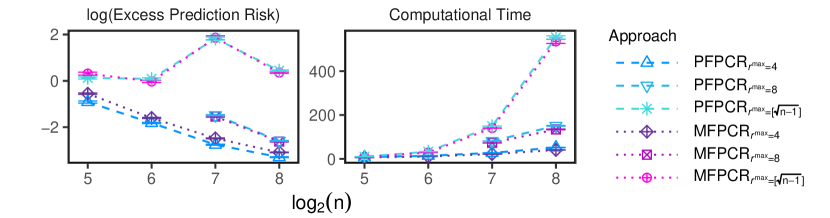
Figure E.1: Plots of the excess prediction risk and computational time vs. the sample size in log scale with $r_{c}=1$ under Setting 1. The error bars correspond to mean $\pm$ one SE.

Given the matrix-valued predictor, another natural but undesirable choice is to perform vectorization first and then apply existing methods which apply to vector-valued data. It is known in the literature of tensor data analysis that such vectorization is sub-optimal. With the additional feature of the functional data, to make comprehensive comparison with existing methods, we still include the 1D FLR of Cai and Yuan (2012) after vectorization. In the literature, the default vectorization approach, denoted by vec here, is to stack all the columns of a matrix one by one. In the context of functional data, because of the requirement of smoothness, there are a few other ways of vectorization. For example, it might be worthwhile to consider flipping the even-numbered column vectors upside down and then stack all the columns together, which is denoted by $\textrm{vec}^{*}$. Furthermore, maybe rows are smoother, and so stacking rows (and potentially flipping even-numbered rows) is more appropriate. These considerations lead to four ways of vectorization and result in FLR+$\textrm{vec}(X(s,t))$, FLR+$\textrm{vec}(X^{T}(s,t))$, FLR+$\textrm{vec}^{*}(X(s,t))$ and FLR+$\textrm{vec}^{*}(X^{T}(s,t))$.

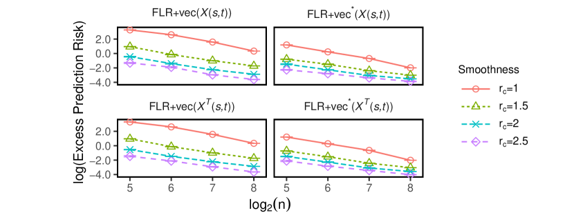
Figure E.2: Plots of the excess prediction risk vs. the sample size with both axes in log scale under Setting 1. Four sample sizes and four values of $r_{c}$ are considered. The error bars correspond to mean $\pm$ one SE. The four panels are for four types of vectorization methods.

The comparison of the four different vectorization approaches is shown in Figure E.2. Because in the simulation setup, the covariances $C_{\alpha},C_{\beta}$ and coefficient functions $\alpha_{0}(\cdot),\beta_{0}(\cdot)$ are symmetric for the two domains, transposing $X$ or not, i.e., stacking rows or columns, does not matter. However, concatenating head-to-tail or head-to-head does matter as revealed in the figure, where the performance of $\textrm{vec}^{*}$ dominates that of vec.

For these reasons, for the rest of this section, FLR refers to FLR+$\textrm{vec}^{*}(X(s,t))$; in Section 5 on the Canadian weather data, FLR refers to FLR+$\textrm{vec}(X^{T}(s,t))$, because it is natural to connect the last hour in the current day to the first hour in the next day; in Section G on the LIDAR data, where the two domains are different, we consider two choices: FLR+$\textrm{vec}^{*}(X(s,t))$ and FLR+$\textrm{vec}^{*}(X^{T}(s,t))$.

Lastly, besides GMRF, PFPCR and MFPCR, we also compare the performance of FBLR with three more existing methods: FLR, Ridge regression after plain vectorization, and BLR (a special case of FBLR when $\lambda_{\alpha}=\lambda_{\beta}=0$). Figure E.3 shows the clear advantage of FBLR over them due to their lack of smoothness or lack of matrix structure.

Figure E.3: Plots of the excess prediction risk vs. the sample size in log scale for Settings 1. Four approaches are included. The error bars are generated according to mean $\pm$ one SE. BLR is only shown for $\log_{2}(n)=7,8$, because it requires a larger sample size.

Appendix F Additional real data analysis on Canadian weather

This section provides more information on the application to the Canadian weather data as a supplement to Section 5. Figure F.1 provides the residual diagnosis of FBLR, which suggests a fairly good fit of the data.

Figure F.1: The diagnosis plots of the residuals of FBLR for the Canadian weather data.

Appendix G Real data analysis: LIDAR

We demonstrate the performance of FBLR and other methods on the LIDAR data. The goal is to discriminate biological threat aerosol clouds in the atmosphere from non-biological interferent aerosol clouds such as dust or smoke. We use the same dataset as in Xun et al. (2013), where there are 28 aerosol clouds, half being biological and the other half non-biological. For each aerosol cloud at each time point, a set of 19 wavelength pulses is transmitted. The LIDAR receiver collects a fraction of the total optical power back-scattered over 60 equally-spaced range points (excluding background) at time $1,2,\ldots,20$ for wavelength $1,2,\ldots,19$. See Figure G.1 for an illustration of the data generation process.

Figure G.1: A comic describing the LIDAR data generation.

Figure G.2 provides some visualization for one biological sample. It shows that the signal is smooth along three domains: time, range, and wavelength. In the literature of chemical biology, researchers have used approaches such as support vector machines after feature engineering or partial differential equation to solve this problem. Because of the smoothness of the surface, we will apply functional methods instead.

Figure G.2: Snapshots of one biological sample in the LIDAR data. 20 curves correspond to 20 time points. The left panel is the received signal over all 60 ranges at wavelength value 11. The right panel is the received signal over all 19 wavelengths at range value 45.

Ideally, one should use 3D input of size $60\times 19\times 20$ as the predictor to make prediction. Given that FBLR and most existing methods only apply to 2D data, we will perform the analysis 20 times corresponding to 20 time points separately. For each time point, we have 28 observations with input $x_{i}$ of size $60\times 19$ and response $y_{i}$ taking value 0 or 1, standing for non-biological or biological aerosol, respectively. We adopt the regression approach to make classification: assign to class 1 if and only if the predicted response is larger than .5. We use leave-one-out method to compute the out-of-sample testing misclassification rate. The boxplots of 20 testing misclassification rates for 20 time points and computational time for eight approaches are given in Figure G.3.

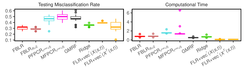
Figure G.3: Boxplots of the testing misclassification rates and computation time of 20 time points for multiple approaches in the LIDAR data.

Both FBLR and ${\rm FBLR}_{R=2}$ are included. We perform the test on the separability of the covariance by using Aston et al. (2017) and the separability is verified for all time points. As explained in Appendix E, FLR with two types of vectorization is compared with. For FBLR-related and FLR-related methods, we use the kernel in (17) again. For PFPCR and MFPCR, we set $r^{\max}=\lfloor\sqrt{n-1}\rfloor=5$. BLR is not included because the sample size is not large enough. Figure G.3 shows that ${\rm FBLR}_{R=2}$ is the best, followed by FBLR. The other 2D methods such as PFPCR, MFPCR and GMRF are close to random guesses and even worse than the 1D methods such as FLR+$\textrm{vec}^{*}(X(s,t))$, FLR+$\textrm{vec}^{*}(X^{T}(s,t))$ and Ridge.

Figures G.4 - G.7 further show the advantage of FBLR over other methods on LIDAR data in terms of interpretation, smoothness, and stableness. Figure G.4 shows the heat-maps of the estimated 2D coefficient function $\hat{\beta}(\cdot,\cdot)$ in Model (3) for these eight methods at time point 2, which is randomly selected (the other time points have similar message). It shows that both FBLR and ${\rm FBLR}_{R=2}$ obtain smoother coefficient function estimations compared with other 2D methods. The small visual difference between FBLR and ${\rm FBLR}_{R=2}$ indicates that the second term in Model (4) has a small magnitude. Furthermore, although PFPCR and MFPCR are supposed to provide smooth estimations, the resulting estimated coefficient function is not very smooth. For the 1D methods, Ridge estimation inherently lacks smoothness, and FLR+$\textrm{vec}^{*}(X(s,t))$ (stacking columns) and FLR+$\textrm{vec}^{*}(X^{T}(s,t))$ (stacking rows) exhibit excessive smoothing because one dimension has nearly no variation.

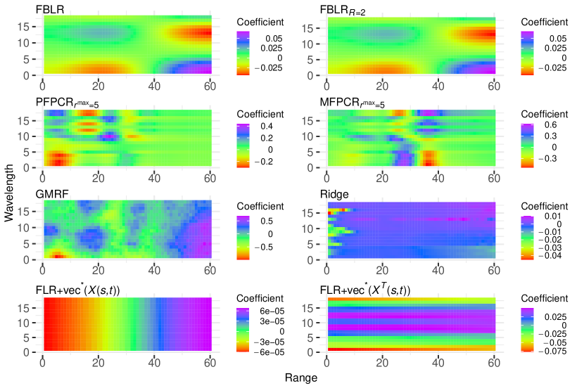
Figure G.4: Plots of the estimated 2D coefficient function $\hat{\beta}(\cdot,\cdot)$ in Model (3) for LIDAR data at time point 2. The two axes correspond to range and wavelength, respectively.

Figure G.5 shows the estimated 2D coefficient functions $\hat{\beta}(\cdot,\cdot)$ in Model (3) by ${\rm FBLR}_{R=2}$ for LIDAR data at 20 time points. Every 2D coefficient function at any time point is smooth and the 2D coefficient functions evolve smoothly over time.

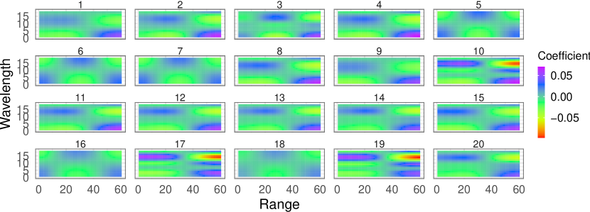
Figure G.5: Plots of the estimated 2D coefficient functions $\hat{\beta}(\cdot,\cdot)$ in Model (3) by ${\rm FBLR}_{R=2}$ for LIDAR data at 20 time points. The two axes correspond to range and wavelength.

We next compare the evolvement of the 2D coefficient functions over time of all eight methods. A direct comparison of the 2D surfaces is difficult, so we perform SVD of all 2D coefficient functions. Figures G.6 - G.7 show the leading left and right singular vectors, which correspond to $\hat{\alpha}^{[1]}(\cdot)$ and $\hat{\beta}^{[1]}(\cdot)$ in Model (2), respectively. Again, the estimated 1D coefficient functions by FBLR and ${\rm FBLR}_{R=2}$ are smooth for each time point and evolve smoothly over time; in contrast, the estimated 1D coefficient functions by 2D methods such as PFPCR, MFPCR, and GMRF are in general not very smooth for each time point and do not evolve quite smoothly over time; the estimated 1D coefficient functions by 1D methods such as FLR+$\textrm{vec}^{*}(X(s,t))$ and FLR+$\textrm{vec}^{*}(X^{T}(s,t))$ tend to be over-smoothed for one of the two domains. This demonstrates the “stableness” of the (iterative) FBLR estimations.

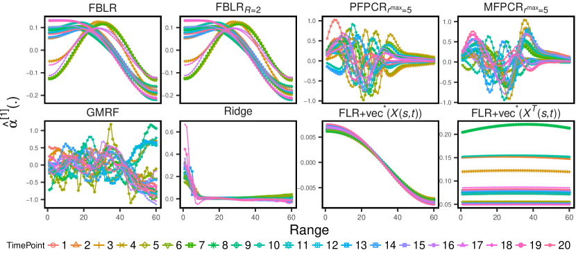
Figure G.6: Plots of the estimated 1D coefficient function $\hat{\alpha}^{[1]}(\cdot)$ that corresponds to the range domain in Model (2). 20 curves in each panel correspond to 20 time points.

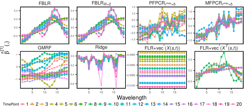
Figure G.7: Plots of the estimated 1D coefficient function $\hat{\beta}^{[1]}(\cdot)$ that corresponds to the wavelength domain in Model (2). 20 curves in each panel correspond to 20 time points.

References

• Aston etΒ al. (2017) J.Β A. Aston, D.Β Pigoli, and S.Β Tavakoli. Tests for separability in nonparametric covariance operators of random surfaces. The Annals of Statistics, pages 1431–1461, 2017.
• Bi etΒ al. (2018) X.Β Bi, A.Β Qu, and X.Β Shen. Multilayer tensor factorization with applications to recommender systems. The Annals of Statistics, 46(6B):3308–3333, 2018.
• Bi etΒ al. (2021) X.Β Bi, X.Β Tang, Y.Β Yuan, Y.Β Zhang, and A.Β Qu. Tensors in statistics. Annual review of statistics and its application, 8:345–368, 2021.
• Cai and Hall (2006) T.Β T. Cai and P.Β Hall. Prediction in functional linear regression. The Annals of Statistics, 34(5):2159–2179, 2006.
• Cai and Yuan (2012) T.Β T. Cai and M.Β Yuan. Minimax and adaptive prediction for functional linear regression. Journal of the American Statistical Association, 107(499):1201–1216, 2012.
• Chen and MΓΌller (2012) K.Β Chen and H.Β G. MΓΌller. Modeling repeated functional observations. Journal of the American Statistical Association, 107(500):1599–1609, 2012.
• Chen etΒ al. (2017) K.Β Chen, P.Β Delicado, and H.Β G. MΓΌller. Modelling function-valued stochastic processes, with applications to fertility dynamics. Journal of the Royal Statistical Society Series B: Statistical Methodology, 79(1):177–196, 2017.
• Chen etΒ al. (2021) R.Β Chen, H.Β Xiao, and D.Β Yang. Autoregressive models for matrix-valued time series. Journal of Econometrics, 222(1):539–560, 2021.
• Chen etΒ al. (2022) R.Β Chen, D.Β Yang, and C.Β H. Zhang. Factor models for high-dimensional tensor time series. Journal of the American Statistical Association, 117(537):94–116, 2022.
• Chen etΒ al. (2023) X.Β Chen, D.Β Yang, Y.Β Xu, Y.Β Xia, D.Β Wang, and H.Β Shen. Testing and support recovery of correlation structures for matrix-valued observations with an application to stock market data. Journal of Econometrics, 232(2):544–564, 2023.
• Donohoe etΒ al. (2020) A.Β Donohoe, E.Β Dawson, L.Β McMurdie, D.Β S. Battisti, and A.Β Rhines. Seasonal asymmetries in the lag between insolation and surface temperature. Journal of Climate, 33(10):3921–3945, 2020.
• Dyrholm etΒ al. (2007) M.Β Dyrholm, C.Β Christoforou, and L.Β C. Parra. Bilinear discriminant component analysis. Journal of Machine Learning Research, 8:1097–1111, 2007.
• Gu (2013) C.Β Gu. Smoothing spline ANOVA models, volume 297. Springer Science and Business Media, 2013.
• Guillas and Lai (2010) S.Β Guillas and M.-J. Lai. Bivariate splines for spatial functional regression models. Journal of Nonparametric Statistics, 22:477–497, 2010.
• Hafner etΒ al. (2020) C.Β M. Hafner, O.Β B. Linton, and H.Β Tang. Estimation of a multiplicative correlation structure in the large dimensional case. Journal of Econometrics, 217(2):431–470, 2020.
• Happ etΒ al. (2018) C.Β Happ, S.Β Greven, and V.Β J. Schmid. The impact of model assumptions in scalar-on-image regression. Statistics in medicine, 37(28):4298–4317, 2018.
• Hoff (2015) P.Β D. Hoff. Multilinear tensor regression for longitudinal relational data. The annals of applied statistics, 9(3):1169, 2015.
• Huang etΒ al. (2009) J.Β Z. Huang, H.Β Shen, and A.Β Buja. The Analysis of Two-Way Functional Data Using Two-Way Regularized Singular Value Decompositions. Journal of the American Statistical Association, 104(488):1609–1620, 2009.
• Kang etΒ al. (2018) J.Β Kang, B.Β J. Reich, and A.Β M. Staicu. Scalar-on-image regression via the soft-thresholded gaussian process. Biometrika, 105(1):165–184, 2018.
• Liu etΒ al. (2019) J.Β Liu, Z.Β Wu, L.Β Xiao, J.Β Sun, and H.Β Yan. Generalized tensor regression for hyperspectral image classification. IEEE Transactions on Geoscience and Remote Sensing, 58(2):1244–1258, 2019.
• Micchelli and Wahba (1981) C.Β A. Micchelli and G.Β Wahba. Design problems for optimal surface interpolation. In Approximation Theory and Applications, pages 329–348. Academic Press, New York, 1981.
• Park and Staicu (2015) S.Β Y. Park and A.Β M. Staicu. Longitudinal functional data analysis. Stat, 4(1):212–226, 2015.
• Ramsay and Dalzell (1991) J.Β O. Ramsay and C.Β J. Dalzell. Some Tools for Functional Data Analysis (with discussion). Journal of the Royal Statistical Society: Series B (Statistical Methodology), 53(3):539–572, 1991.
• Ramsay and Silverman (2002) J.Β O. Ramsay and B.Β W. Silverman. Applied Functional Data Analysis: Methods and Case Studies. Springer, New York, NY, 2002.
• Ramsay and Silverman (2005a) J.Β O. Ramsay and B.Β W. Silverman. Functional Data Analysis. Springer, New York, NY, 2nd edition, 2005a.
• Ramsay and Silverman (2005b) J.Β O. Ramsay and B.Β W. Silverman. Principal components analysis for functional data. Functional data analysis, pages 147–172, 2005b.
• Reiss and Ogden (2010) P.Β T. Reiss and R.Β T. Ogden. Functional Generalized Linear Models with Images as Predictors. Biometrics, 66(1):61–69, 2010.
• Reiss etΒ al. (2015) P.Β T. Reiss, L.Β Huo, Y.Β Zhao, C.Β Kelly, and R.Β T. Ogden. Wavelet-domain regression and predictive inference in psychiatric neuroimaging. The Annals of Applied Statistics, 9(2):1076–1101, 2015.
• Reiss etΒ al. (2017) P.Β T. Reiss, J.Β Goldsmith, H.Β L. Shang, and R.Β T. Ogden. Methods for scalar-on-function regression. International Statistical Review, 85(2):228–249, 2017.
• Sacks and Ylvisaker (1968) J.Β Sacks and D.Β Ylvisaker. Designs for regression problems with correlated errors; many parameters. The Annals of Mathematical Statistics, 39:49–69, 1968.
• Sacks and Ylvisaker (1970) J.Β Sacks and D.Β Ylvisaker. Designs for regression problems with correlated errors III. The Annals of Mathematical Statistics, 41:2057–2074, 1970.
• Sacks and Ylvisaker (1966) J.Β Sacks and N.Β D. Ylvisaker. Designs for regression problems with correlated errors. The Annals of Mathematical Statistics, 37:66–89, 1966.
• Sangalli etΒ al. (2013) L.Β M. Sangalli, J.Β O. Ramsay, and T.Β O. Ramsay. Spatial spline regression models. Journal of the Royal Statistical Society: Series B (Statistical Methodology), 75(4):681–703, 2013.
• Sun and Li (2017) W.Β W. Sun and L.Β Li. Store: sparse tensor response regression and neuroimaging analysis. The Journal of Machine Learning Research, 18(1):4908–4944, 2017.
• Tsybakov (2009) A.Β B. Tsybakov. Introduction to Nonparametric Estimation. Springer, New York, 2009.
• Volfovsky and Hoff (2015) A.Β Volfovsky and P.Β D. Hoff. Testing for nodal dependence in relational data matrices. Journal of the American Statistical Association, 110(511):1037–1046, 2015.
• Wahba (1990) G.Β Wahba. Spline models for observational data. SIAM, Philadelphia, PA, 1990.
• Wang etΒ al. (2016) J.Β L. Wang, J.Β M. Chiou, and H.Β G. MΓΌller. Functional Data Analysis. Annual Review of Statistics and Its Application, 3:257–295, 2016.
• Wang etΒ al. (2014) X.Β Wang, B.Β Nan, J.Β Zhu, and R.Β Koeppe. Regularized 3D functional regression for brain image data via Haar wavelets. The Annals of Applied Statistics, 8(2):1045–1064, 2014.
• Werner etΒ al. (2008) K.Β Werner, M.Β Jansson, and P.Β Stoica. On estimation of covariance matrices with Kronecker product structure. IEEE Transactions on Signal Processing, 56(2):478–491, 2008.
• Xiao etΒ al. (2013) L.Β Xiao, Y.Β Li, and D.Β Ruppert. Fast bivariate p-splines: the sandwich smoother. Journal of the Royal Statistical Society: Series B (Statistical Methodology), 75(3):577–599, 2013.
• Xun etΒ al. (2013) X.Β Xun, J.Β Cao, B.Β Mallick, A.Β Maity, and R.Β J. Carroll. Parameter estimation of partial differential equation models. Journal of the American Statistical Association, 108(503):1009–1020, 2013.
• Yang and Smith (2006) S.Β Yang and E.Β A. Smith. Mechanisms for diurnal variability of global tropical rainfall observed from trmm. Journal of climate, 19(20):5190–5226, 2006.
• Yuan and Cai (2010) M.Β Yuan and T.Β T. Cai. A reproducing kernel hilbert space approach to functional linear regression. The Annals of Statistics, 38(6):3412–3444, 2010.
• Zhou etΒ al. (2013) H.Β Zhou, L.Β Li, and H.Β Zhu. Tensor regression with applications in neuroimaging data analysis. Journal of the American Statistical Association, 108(502):540–552, 2013.
• Zhou etΒ al. (2021) J.Β Zhou, W.Β W. Sun, J.Β Zhang, and L.Β Li. Partially observed dynamic tensor response regression. Journal of the American Statistical Association, pages 1–16, 2021.
• Zhou (2014) S.Β Zhou. Gemini: Graph estimation with matrix variate normal instances. The Annals of Statistics, 42(2):532–562, 2014.
Supplement to β€œOptimal Functional Bilinear Regression with Two-way Functional Covariates via Reproducing Kernel Hilbert Space”
Dan Yang, Jianlong Shao, Haipeng Shen, Dong Wang, and Hongtu Zhu