The mass-radius relation of exoplanets, revisited

Determining the mass-radius ($M$-$R$) relation of exoplanets is important for exoplanet characterization. Here we present a re-analysis of the $M$-$R$ relations and their transitions using exoplanetary data from the PlanetS catalog which accounts only for planets with reliable mass and radius determination. We find that ”small planets” correspond to planets with masses of up to $7.80^{+9.74}_{-4.33}M_{\oplus}$ where $R\propto M^{0.41\pm 0.09}$. Planets with masses between $7.80^{+9.74}_{-4.33}M_{\oplus}$ and $125^{+11}_{-10}M_{\oplus}$ can be viewed as ”intermediate-mass” planets, where $R\propto M^{0.65\pm 0.03}$. Massive planets, or gas giant planets, are found to have masses beyond $125^{+11}_{-10}M_{\oplus}$ with an $M$-$R$ relation of $R\propto M^{-0.02\pm 0.01}$. By analyzing the radius-density relation we also find that the transition between ”small” to ”intermediate-size” planets occurs at a planetary radius of $1.69^{+0.45}_{-0.35}R_{\oplus}$. Our results are consistent with previous studies and provide an ideal fit for the currently-measured planetary population.

1 Introduction

Since the detection of the first exoplanet around a sun-like star in 1995 (Mayor & Queloz 1995) over 5000 exoplanets have been discovered revealing a large diversity in their physical properties. The field of exoplanet is blossoming and we are at a stage where we move from exoplanet detection to exoplanet characterization, with both of these fronts being extremely active and reaching a new level. When it comes to exoplanet characterization, the two fundamental parameters are the planetary mass and radius. However, these two properties cannot be measured by the same method, and unfortunately in many cases only one of the two is available. To allow for a broader overview of exoplanets in a statistical sense, it is valuable to determine their mass-radius ($M$-$R$) relation and how this relation changes for different planetary types. The ability to relate a measured radius to a planet’s mass can also help with radial-velocity follow-ups by estimating the expected radial velocity semi-amplitude of a transiting exoplanet.

The $M$-$R$ relation depends on the planetary composition and therefore on the behavior of the different materials at planetary conditions (e.g., Seager et al. 2007; Chabrier et al. 2009; Grasset et al. 2009; Mordasini et al. 2012; Spiegel et al. 2014a; Jontof-Hutter 2019). Theoretical $M$-$R$ relations can be inferred from interior models that rely on equations of state (EOS), which relate the density and pressure (and in general also the temperature) of a given composition. For simplicity, often small terrestrial planets are assumed to have constant densities and are thus expected to behave as $R\propto M^{1/3}$ (e.g., Spiegel et al. 2014b). On the other hand, in massive giant planets that are hydrogen-helium (H-He) dominated in composition, the gravitational pressure is high enough for the materials to be pressure ionized and the electron degeneracy pressure becomes substantial (e.g., Helled et al. 2020). In that case, the radius would decrease with increasing mass, with $R\propto M^{-1/3}$. Of course, the planetary radius does not only depend on its mass but also other factors like stellar irradiation or the planetary age.

Nowadays there are enough planets with both mass and radius measurements to statistically infer an observed $M$-$R$ relation. The observed $M$-$R$ relations of exoplanets have been investigated in several studies and are often fitted by a broken power law. The breakpoints are of particular interest as they represent the transitions between different planetary types. For example, Weiss et al. (2013) inferred a mass-radius-incident-flux relation. Based solely on the visual inspection of the $M$-$R$ and mass-density ($M-\rho$) diagrams, they found a transition point at $150M_{\oplus}$. They inferred relations $R\propto M^{0.53}F^{-0.03}$ for $M<150M_{\oplus}$ and $R\propto M^{-0.04}F^{0.09}$ for $M>150M_{\oplus}$, where $F$ is the instellation flux. With this, they suggested that for small planets the mass is the most important parameter for predicting the planetary radius, whereas for giant planets it seems that the incident flux is more important. Below $150M_{\oplus}$ only the data of 35 planets was available at the time, and therefore the result for this region is less robust.

A different approach was taken by Hatzes & Rauer (2015). In this study, the transition for giant planets has been explored. They used observations to infer the $M-\rho$ relation. A minimum in density at $\simeq 95M_{\oplus}$ ($0.3M_{J}$) and a maximum at $\simeq 1.9\times 10^{4}M_{\oplus}$ ($60M_{J}$) were inferred, suggesting that these values correspond to the transition into gas giant planets. This study also suggested that there is no separation between brown dwarfs and giant planets as they display similar behavior. The mass-density relation of giant planets was determined to be $\rho=0.78M^{1.15}$.

Chen & Kipping (2017) presented an elaborate Markov Chain Monte Carlo method to analyze the $M$-$R$ relations of objects ranging from dwarf planets to stars. They inferred four distinct regions in their work: Terran worlds, Neptunian worlds, Jovian worlds, and stars. The corresponding transition points were fitted for and identified as 2.04, 132, and 2.66 $\times 10^{4}M_{\oplus}$, where the latter two values correspond to $0.41M_{J}$ and $0.08M_{\odot}$. The $M$-$R$ relations were identified as: $R\propto M^{0.28}$ for Terran worlds, $R\propto M^{0.59}$ for Neptunian worlds, $R\propto M^{-0.04}$ for Jovian worlds and $R\propto M^{0.88}$ for stars. The results were obtained by a solely data-driven analysis rather than being derived from any physical assumptions. At the time of the study, only a few objects at $\sim 1M_{\oplus}$ had been observed, and therefore the transition point between the Terran and Neptunian worlds relied on a relatively small number of planets.

Bashi et al. (2017) fitted the $M$-$R$ relations of two distinct regions by using a total least squares approach, where the transition point was set to be unknown. It was found that the transition occurs at $\sim 124M_{\oplus}$ and $12.1R_{\oplus}$. The data was best fitted by the relations: $R\propto M^{0.55}$ for small planets and $R\propto M^{0.01}$ for large planets. In this study, the transition point was also fitted instead of being imposed by some prior assumption.

Recently, Otegi et al. (2020) presented an updated catalog of exoplanets, for which robust measurements of both radius and mass are available, based on the NASA Exoplanet Archive catalogue. The goal of their work was to find the transition between rocky planets and those with a substantial gas envelope, and therefore only planets with masses up to $120M_{\oplus}$ were considered. When displaying the planets in the $M$-$R$ plane, two distinct regions could be identified: the rocky and the volatile-rich populations. Because they overlap in both mass and radius, the populations have been separated by the pure-water composition line to distinguish volatile-rich planets from terrestrial ones. For the distinct groups, the following ($M$-$R$) relations were inferred: $R=1.03M^{0.29}$ for the rocky population and $R=0.70M^{0.63}$ for the volatile-rich population.

Edmondson et al. (2023) showed that a discontinuous $M$-$R$ relation as well as a temperature dependence for giant planets results in a good fit to the $M$-$R$ measurements. Similar to Otegi et al. (2020) they separate between the rocky and the icy planets by a pure-ice EOS, while finding the transition of icy planets to gas giants at $115M_{\oplus}$. For the rocky planets, they fit a relation of $R\propto M^{0.34}$ and for the icy planets $R\propto M^{0.55}$. When also considering the equilibrium temperature of the gas giants they find that $R\propto M^{0.00}T^{0.35}$ suggesting that for the giant planets, the radius only depends on the temperature.

Recently, Mousavi-Sadr et al. (2023) used a machine-learning approach to analyze the exoplanet population. By applying various clustering algorithms they identified the transition between ”small” and giant planets at masses of $52.48M_{\oplus}$ and sizes of $8.13R_{\oplus}$. For the small planets, the $M$-$R$ relation was found to be $R\propto M^{0.50}$. They also showed that the radii of giant planets are positively correlated with the stellar mass.

In this paper, we investigate the $M$-$R$ relations of exoplanets and their transitions using the PlanetS catalog. We use a solely statistical approach to determine the breakpoints in the relation used to define the different planetary regimes and determine the distinct dependencies. We also analyze the mass-density ($M$-$\rho$) and radius-density ($R$-$\rho$) relations and investigate their validity in separating different planetary types.

2 Methods

In this work, we use the data from the PlanetS Catalog. An earlier version was presented in Otegi et al. (2020); since then the catalog has been extended with additional discoveries and planets with masses up to $30M_{J}$. There has also been an update on the planetary masses, and some planetary parameters have been reanalyzed. The catalog only includes planets with relative measurement uncertainties on the mass smaller than 25% and the radius smaller than 8%. Since the updated catalog contains many more planets, it is more reliable and allows for additional analyses. The data we’ve used was downloaded in July 2023 and contains the mass and radius measurements of 688 exoplanets. Fig. 1 shows how the planets are distributed in the ($M$-$R$) plane.

Similar to previous work, our approach was to assume that there is a power-law relation between two planetary variables, for example, $M$ and $R$. The first step was to transform the variables into the log-log plane to use a linear regression method. We further assumed that there is an unknown number of break points in the linear relation between the two log-transformed variables, i.e., that a piece-wise linear function describes the data. To perform the fit we used the piecewise-regression Python package (Pilgrim 2021), which is based on the method described in Muggeo (2003). To determine the number of breakpoints, we fit piece-wise linear functions with various numbers of breakpoints to the data. Then, we used the Bayesian Information Criterion (BIC) to compare the models. The model with the lowest BIC is the best description of the data and therefore yields the best-fit number of breakpoints.

For one break point, the piece-wise linear function is (Pilgrim 2021):

$$y=\cases{c}+\alpha_{1}\xi&\xi<\psi_{1}\\ c-\beta_{1}\psi_{1}+\alpha_{2}\xi\xi>\psi_{1}{}$$ (1)

Similarly, for two break points, the piece-wise linear function is given by (Pilgrim 2021):

$$y=\cases{c}+\alpha_{1}\xi&\xi<\psi_{1}\\ c-\beta_{1}\psi_{1}+\alpha_{2}\xi\psi_{1}<\xi<\psi_{2}\\ c-\beta_{1}\psi_{1}-\beta_{2}\psi_{2}+\alpha_{3}\xi\psi_{2}<\xi{}$$ (2)

The piece-wise linear functions with more breakpoints follow a similar pattern. The independent and dependent variables are $\xi$ and $y$, respectively. For the $M$-$R$ relation, $\xi\equiv\log(M[M_{\oplus}])$ and $y\equiv\log(R[R_{\oplus}])$, for the $M$-$\rho$ relation $xi\equiv\log(M[M_{\oplus}])$ and $y\equiv\log\rho$ [g/cm³], and for the $R$-$rho$ relation $xi\equiv\log(R[R_{\oplus}])$ and $\xi\equiv\log\rho$ [g/cm³]. The parameters of the piece-wise linear functions are $c$, $\alpha_{i}$, $\beta_{i}$, and $\psi_{i}$. The constant $c$ is the intercept of the first segment, $\beta_{1,2}$ are the changes in gradients, $\alpha_{1,2,3}$ are the gradients of the three segments, and $\psi_{1,2}$ are the two breakpoints. Note that $\alpha_{2,3}$ are not independent, but are calculated from $\alpha_{1}$ and $\beta_{1,2}$.

The planetary bulk density was calculated using $\rho=\frac{3M}{4\pi R^{3}}$ and its uncertainty was inferred using a simple error-propagation:

$$\begin{split}\sigma_{\rho}^{2}{}&=\left|\frac{\partial\rho}{\partial M}\right|^{2}\sigma_{M}^{2}+\left|\frac{\partial\rho}{\partial R}\right|^{2}\sigma_{R}^{2}\\ &=\left(\frac{3}{4\pi R^{3}}\right)^{2}\sigma_{M}^{2}+\left(\frac{9M}{4\pi R^{4}}\right)^{2}\sigma_{R}^{2}.\end{split}$$ (3)

To include the measurement uncertainties on $M$ and $R$ (and therefore $\rho$; see 3) in the fits, we used a re-sampling method: We randomly created a large number ($N$) of new data sets by sampling the planets from their observed prior distributions. We assumed that data were normally distributed around their mean measurement values, with the errors given by the uncertainties. Since the fits were performed in log-log space, the measurement uncertainties needed to be converted into their logarithmic form via the following transformations:

$$\begin{split}\sigma_{\text{upper}}(\log x){}&=\log(x+\sigma_{\text{upper}}(x))-\log x\\ &=\log(1+\frac{\sigma_{\text{upper}}(x)}{x})\end{split}$$ (4)

$$\begin{split}\sigma_{\text{lower}}(\log x){}&=\log x-\log(x-\sigma_{\text{lower}}(x))\\ &=\log(\frac{x}{x-\sigma_{\text{lower}}(x)})\end{split}$$ (5)

Here, $x$ is the measured mass or radius, and $\sigma_{upper}$ and $\sigma_{lower}$ are the potentially asymmetric uncertainties. To generate the normal distributions, we used the average of the upper and lower logarithmic errors as the standard deviation. For each new data set, the parameters of the piece-wise linear regression were fitted. From these $N$ sets of parameters, the best fit was obtained by taking the weighted average $\mu_{x}$ and standard deviation $\sigma_{(}\mu_{x})$ like so:

$$\mu_{x}=\frac{\sum_{i}\sigma_{i}^{-2}x_{i}}{\sum_{i}\sigma_{i}^{-2}}\,,\quad\sigma(\mu_{x})=\left(\frac{\sum_{i}\sigma_{i}^{-2}(x_{i}-\mu_{x})^{2}}{N^{-1}(N-1)\sum_{i}\sigma_{i}^{-2}}\right)^{1/2}\,,$$ (6)

where $x$ is one of the fitting parameters from Eq. 1 or 2, $x_{i}$ are the results from the individual fit of each sample, and $\sigma_{i}$ are the corresponding uncertainties. For large $N$, the prefactor $(N-1)/N\approx 1$ can be neglected. We performed a convergence study on the number of samples and settled on $N=10,000$. The details are in Appendix A.

3 Results

In this section, we first present our results for the $M$-$R$, $M$-$\rho$ and $R$-$\rho$ relations in Subsections 3.1, 3.2 and 3.3. We then compare our results to previous studies in Subsection 3.3.1.

3.1 The mass-radius relation

By comparing the BIC of models with different numbers of breakpoints, we found that a piece-wise linear relation with two breakpoints provided the best fit to the $M$-$R$ distribution of the exoplanets from the PlanetS Catalog. This led to the following $M$-$R$ relation:

$$R(M)=\cases{1}.00^{+0.06}_{-0.06}M^{0.41\pm 0.09}&M<7.80^{+9.74}_{-4.33}\\ 0.55^{+0.17}_{-0.18}M^{0.65\pm 0.03}7.80^{+9.74}_{-4.33}<M<125^{+11}_{-10}\\ 14.3^{+5.60}_{-5.20}M^{-0.02\pm 0.01}M>125^{+11}_{-10}{}$$ (7)

where $R$ and $M$ are in Earth units. The piece-wise linear fit with two breakpoints is shown together with the data in Fig. 1, and the fit parameters (see Eq. 2) are listed in Table 1.

Figure 1: The data from the PlanetS Catalog is displayed in blue. The mass-radius relation we find (Equation 7) is displayed as the solid black line with the shaded region as the $1\sigma$ confidence interval. The positions of the corresponding breakpoints are shown as the dashed line.

Our $M$-$R$ fit with two breakpoints was split into three different regimes (segments): They correspond to small planets ($M<7.80M_{\oplus}$), intermediate-mass planets ($7.80M_{\oplus}<M<125M_{\oplus}$) and giant planets ($M>125M_{\oplus}$). The first breakpoint has a high uncertainty, with a transition mass of $M_{1}=7.80^{+9.74}_{-4.33}M_{\oplus}$. Between the first and second segments, there is only a small change in the gradient, making it harder to identify the location of the breakpoint. We find that the fit is particularly suitable for determining the second breakpoint with low uncertainty ($M_{2}=125^{+11}_{-10}M_{\oplus}$) and describing the data in the second segment. The description of the data in the third segment (the giant planets) is also relatively uncertain: The planets in the third segment show a large scatter, making it difficult to find a well-fitting gradient.

Parameter	Value
$c$	$0.00\pm 0.03$
$\beta_{1}$	$0.29\pm 0.08$
$\beta_{2}$	$-0.67\pm 0.03$
$\alpha_{1}$	$0.41\pm 0.09$
$\alpha_{2}$	$0.65\pm 0.03$
$\alpha_{3}$	$-0.02\pm 0.01$
$\psi_{1}$	$0.89\pm 0.35$
$\psi_{2}$	$2.10\pm 0.04$

Table 1: Results for the parameters in Equation (2) from fitting the exoplanetary mass ($\log(M[M_{\oplus}])$) and radius ($\log(R[R_{\oplus}])$) data. The values were rounded to two decimal places.

The first regime of exoplanets corresponds to planets with masses below $\simeq 7.80M_{\oplus}$ and roughly follows the relation of $R\propto M^{0.41}$. However, as noted above, the transition mass is rather uncertain. These planets are most likely ”rocky worlds” with compositions similar to the Earth’s. If terrestrial planets can be approximated as constant-density homogeneous spheres, they would follow the simple relation $R\propto M^{1/3}$, which is similar to what we find. The scatter around this relation in the actual data comes from the differential structure of planets and the diversity in their bulk densities, i.e., rocks-to-metals ratios and the possible existence of lighter elements such as water (e.g., Seager et al. 2007; Weiss et al. 2013; Zeng et al. 2016).

The change in the slope around $7.80M_{\oplus}$ defines the transition to the intermediate-mass planets, which could also have non-negligible H-He envelopes. Our fit to the data implies that the maximal mass of ”rocky” exoplanets and possibly of naked planetary cores is close to $10M_{\oplus}$. This also implies that the minimum mass to accrete a substantial amount of volatile elements is about $10M_{\oplus}$. The transition region is consistent with the theoretical mass limit of about $10M_{\oplus}$ for ”rocky” exoplanets (e.g., Seager et al. 2007; Fortney et al. 2007; Charbonneau et al. 2009). The intermediate-mass planets between $7.80M_{\oplus}$ and $125M_{\oplus}$ correspond to planets with H-He envelopes but still with a large heavy-element mass fraction. Since the mass range is large, the diversity of the envelope mass fractions varies significantly and can range from very thin atmospheres to rather gaseous envelopes (e.g, Weiss et al. 2013; Hatzes & Rauer 2015; Ulmer-Moll et al. 2019). These planets have the steepest $M$-$R$ relation following $R\propto M^{0.648}$. An increase in mass results in a significantly larger radius, corresponding mainly to a larger envelope composed of volatile elements. The transition to the gas giants occurs around $125M_{\oplus}$ and is where the planets start to be dominated by the H-He envelope. Interestingly, this transition mass is consistent with the suggested transition mass to giant planets based on recent giant planet formation models (Helled 2023).

As expected from their H-He dominated composition, for the giant planets we find that the radius is nearly independent of mass ($R\propto M^{-0.02}$). For high-mass objects consisting of degenerate electron gas, we expect a relation of $R\propto M^{-1/3}$. In the giant planets, the gas is not completely degenerate, leading to a slightly compressible gas and a deviation from the expected relation. At the same time, we also observe a large scatter in radius due to stellar irradiation, different planetary ages, and metallicities which can strongly affect the radii of gas giants (e.g., Thorngren et al. 2016; Teske et al. 2019; Müller et al. 2020; Müller & Helled 2023).

3.2 The mass-density relation

In this subsection, we present a fit to the mass-density ($M$-$\rho$) relation using the planets from the PlanetS Catalog. As in Subsection 3.1, we first determined the best-fit number of breakpoints. Similar to the $M$-$R$ relation, we found that two breakpoints provided the best fit to the data. The fitting function was therefore given by Eq. 2), with $\xi=\log(M[M_{\oplus}])$ and $y=log(\rho[g/cm^{3}])$. The piece-wise linear function with two breakpoints yielded the following $M$-$\rho$ relation:

$$\rho(M)=\cases{5}.53^{+1.18}_{-0.97}M^{(-0.24\pm 0.31)}&M<6.98^{+9.09}_{-3.95}\\ 30.5^{+7.2}_{-14.5}M^{(-0.93\pm 0.07)}6.98^{+9.09}_{-3.95}<M<127^{+10}_{-9}\\ 1.86^{+0.48}_{-0.24}\times 10^{-3}M^{(1.064\pm 0.033)}M>127^{+10}_{-9}{}$$ (8)

where $\rho$ is in g/cm³ and $M$ in $M_{\oplus}$. The inferred $M$-$\rho$ fit is shown in the top panel of Fig. 2 together with the data. Table 2 lists the values of the fitting parameters. We find that the breakpoints in the $M$-$\rho$ relation are very similar to those found in the $M$-$R$ relation and that the transition from small to intermediate planets has a large uncertainty. The planets in the first segment have a large scatter in the $M$-$\rho$ plane, implying that the planets are rather diverse. As a consequence, there is also a large uncertainty in the slope of the $M$-$\rho$ density for the small planets. As discussed above, terrestrial planets can be approximated by a constant density, which is consistent with what we find within the 1$\sigma$ uncertainty on the slope. However, our derived best fit does not provide a good description for all the small planets especially for planets with $M<1M_{\oplus}$.

Parameter	Value
$c$	$0.74\pm 0.08$
$\beta_{1}$	$-0.87\pm 0.26$
$\beta_{2}$	$2.00\pm 0.07$
$\alpha_{1}$	$-0.24\pm 0.31$
$\alpha_{2}$	$-0.93\pm 0.07$
$\alpha_{3}$	$1.06\pm 0.03$
$\psi_{1}$	$0.84\pm 0.36$
$\psi_{2}$	$2.10\pm 0.03$

Table 2: Results for the parameters in Equation (2) from fitting the exoplanetary mass ($\log(M[M_{\oplus}])$) and density ($\log(\rho[g/cm^{3}])$) data. The values were rounded to two decimal places.

To compare the $M$-$\rho$ to the $M$-$R$ relation (as derived in Subsection 3.1), we converted the density $\rho(M)$ from Eq. 8 to a radius using $R=\left(\frac{4\pi\rho}{3M}\right)^{1/3}$. Since both the $M$-$\rho$ and $M$-$R$ relations were fitted using the same data, they should yield very similar results. This can be seen in the bottom panel of Fig. 2 where both solutions are shown together with the data. Indeed, we find that the $M$-$\rho$ and $M$-$R$ relations have very similar behaviors, and the relation derived from the $M$-$\rho$ fit lies well inside the uncertainty of the fit to the $M$-$R$ distribution. The fact that these relations were consistent while being found separately suggests that our approach yields consistent results. However, both approaches have difficulties in accurately determining the transition mass from small to intermediate-mass exoplanets. In the next subsection, we present a $R$-$\rho$ relation that describes the transition in terms of the planetary radius with a much lower uncertainty.

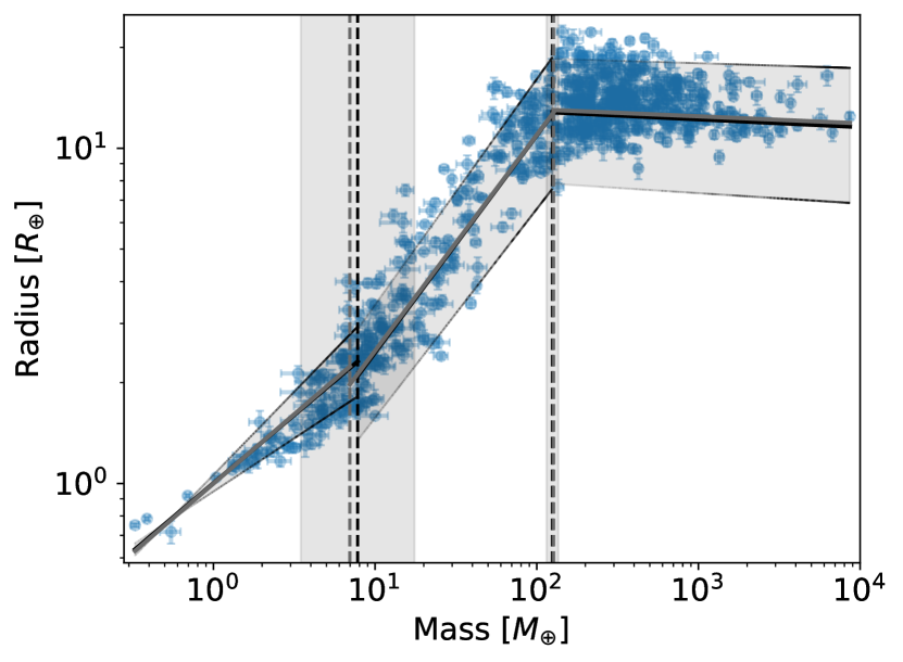
Figure 2: Top: The mass and density data of the exoplanets from the PlanetS Catalog. The mass-density relation is displayed as a solid black line. The dashed lines show the position of the breakpoints. The light-shaded areas are the corresponding $1\sigma$ confidence intervals. Bottom: The mass vs. radius distribution with the best fit for the relation and the breakpoints in black, like in Fig. 1. The grey solid and dashed lines show the mass-radius relation and the corresponding breakpoints derived from the fit to the mass-density distribution.

3.3 The radius-density relation

When fitting the $M$-$R$ and the $M$-$\rho$ relations, the three different regimes were defined by a transition mass. However, it is also possible to search for transitions in the $R$-$\rho$ relation. Here, we calculated the mean density from the measured $M$ and $R$ (see Section 2) and attempted to find a piece-wise linear function that describes the $R$-$\rho$ relation.

The data are shown in the top panel of Fig. 3. Qualitatively, three regimes can be identified in this figure: For the smallest planets, the density seems to be nearly independent of radius. Then, there is a breakpoint where the density decreases steeply with increasing radius. The giant planets (around $13R_{\oplus}$) show a very large dispersion in density. This is similar to what we have already observed in the $M$-$R$ relation of the giant planets. For the giant planets, their bulk density can vary greatly due to their age, instellation flux, and age. The intermediate and the giant planets start to overlap around $7R_{\oplus}$. Therefore, for fitting the $R$-$\rho$ relation, we excluded planets larger than $7R_{\oplus}$.

To describe the $R$-$\rho$ relation, we found that the model with the lowest BIC uses a single breakpoint. This is unlike the two breakpoints for the $M$-$R$ and $M$-$\rho$ relations. However, this is somewhat expected since we excluded the giant planets. The resulting $R$-$\rho$ relation is:

$$\rho(R)=\cases{6}.00^{+1.07}_{-0.90}R^{-0.42\pm 0.82}&R<1.69^{+0.45}_{-0.35}\\ 17.9^{+10.7}_{-7.9}R^{-1.71\pm 0.06}R>1.69^{+0.45}_{-0.35}{}$$ (9)

where $\rho$ and $R$ are in g/cm³ and $R_{\oplus}$, respectively. The $R$-$\rho$ best-fit and the data are shown in the bottom panel of Fig. 3.

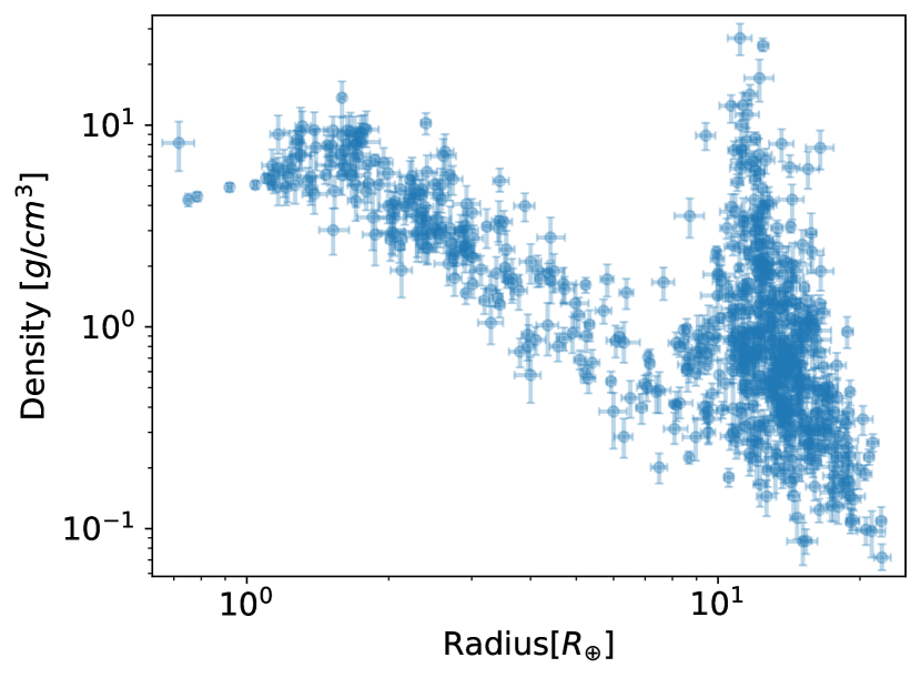
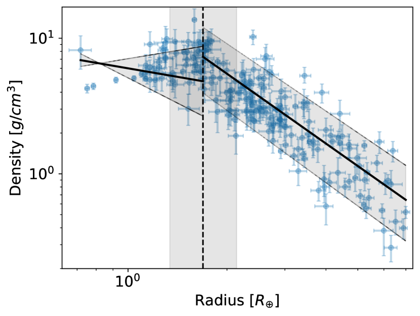
Figure 3: Top: Radius-density distribution of the exoplanets from the PlanetS Catalog. Bottom: The exoplanets from the PlanetS Catalog smaller than $7R_{\oplus}$ are displayed together with the mass-density relation (solid black line) and the corresponding breakpoints (dashed line). The light-shaded areas are the $1\sigma$ confidence intervals.

The values of the parameters for the piece-wise linear function with one breakpoint (see Eq. 1) are listed in Table 3.

Parameter	Value
$c$	$0.78\pm 0.07$
$\beta_{1}$	$-2.08\pm 0.24$
$\alpha_{1}$	$-0.42\pm 0.82$
$\alpha_{2}$	$-1.71\pm 0.06$
$\psi_{1}$	$0.23\pm 0.10$

Table 3: Results for the parameters in Equation (1) from fitting the exoplanetary radius ($\log(R[R_{\oplus}])$) and density ($\log(\rho[g/cm^{3}])$) data. The values were rounded to two decimal places.

An interesting result is the breakpoint at $\sim 1.7R_{\oplus}$. Its relative uncertainty ($\simeq 25\%$) is significantly lower than for the mass threshold between the small and intermediate planets derived from the $M$-$R$ relation ($\simeq 125\%$). This shows that it is beneficial to consider the radius when distinguishing between different planetary types (Rogers 2015; Lozovsky et al. 2018). Similar to the results for the $M$-$\rho$ relation (see Subsection 3.2), we did not find a $R$-$\rho$ relation that provides a good fit for all the planets before the first breakpoint. The inferred slope for the small planets is rather uncertain but is consistent with a constant density approximation within the 1$\sigma$ uncertainty.

Lozovsky et al. (2018) found threshold radii for above which a certain composition is unlikely. For purely rocky planets they found a threshold radius of $1.66^{+0.01}_{-0.08}R_{\oplus}$. Larger planets must consist at least partly of lighter elements, such as H and He. This is consistent with our result of a breakpoint at $\simeq 1.7R_{\oplus}$. However, they only distinguished between super-Earths and mini-Neptunes at $\simeq 3R_{\oplus}$, because planets with a larger radius have a substantial H-He atmosphere (at least $2\%$ mass fraction). In contrast, based on our data no distinction can be made there.

Our result of the radius breakpoint at $\simeq 1.7R_{\oplus}$ also coincides with the position of the radius valley around $1.5-2R_{\oplus}$. The radius valley is a bimodal feature in the occurrence rate of planets as a function of their radii, and the radius valley is seen as a scarcity of planets with $R\simeq 1.5-2R_{\oplus}$. It has been observed for planets with short periods (e.g., Fulton et al. 2017) and is often used for the distinction between super-Earths (below the valley) and mini-Neptunes (above the valley).

Several previous studies have shown how photoevaporation or core-powered mass loss can lead to the depletion of the gaseous envelopes of planets at such radii (Chen & Rogers 2016; Owen & Wu 2017; Venturini et al. 2020), and therefore explain the radius valley. In particular, Kubyshkina & Fossati (2022) suggested that the $M$-$R$ relation of intermediate planets is shaped by their thermal evolution and hydrodynamic escape. Additionally, it has also been suggested that the planets at the upper edge of the radius valley are helium-rich (Malsky et al. 2023). This suggests that due to evaporation of the gaseous envelope for masses with $R\simeq 1.3R_{\oplus}$ planets are naked rocky cores, while around $2.6R_{\oplus}$ they sustain at least part of their H-He envelope. As an alternative, it has also been suggested that the bimodal radius distribution of planets smaller than about $4R_{\oplus}$ is due to different compositions of rocky super-Earths and ice- or water-rich mini-Neptunes (Zeng et al. 2019; Venturini et al. 2020; Izidoro et al. 2021, 2022).

3.3.1 Comparison with previous studies

A comparison of our results with previous studies is presented in Table 4. To facilitate the comparison, the relations and breakpoints were converted to Earth units ($M_{\oplus}$ and $R_{\oplus}$). For the $M$-$R$ relation, we use the results from Subsection 3.1. Also, the mass-density relation from Hatzes & Rauer (2015) was converted to a $M$-$R$ relation. From Edmondson et al. (2023) we chose the $M$-$R$ relation for the giant planets instead of their mass-radius-temperature relation.

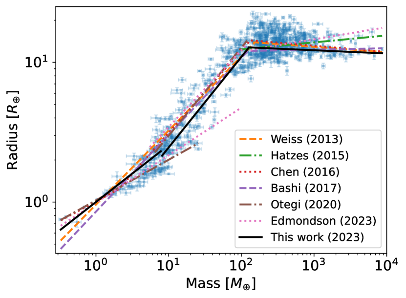
Figure 4: Comparison of the $M$-$R$ relations from different studies with the exoplanetary data from the PlanetS Catalog.

Overall, it is clear that there is a rather good agreement between the various studies despite the use of different methods and data. The $M$-$R$ relations from the different studies are shown in Fig. 4 together with the data from the PlanetS Catalog. It can be seen that the relations from Weiss et al. (2013) and Bashi et al. (2017) underestimate the radii of the smallest planets and are not a good fit. This is because they only use one breakpoint in the $M$-$R$ relation, which corresponds to the transition to giant planets. The relation by Chen & Kipping (2017) does not fit the planets around $10M_{\oplus}$ very well, because the location of the transition from small to intermediate-mass planets is underestimated. Hatzes & Rauer (2015) do not fit planets below $95M_{\oplus}$ at all. The relation by Otegi et al. (2020) remains a good fit for the data set. The main difference to our results is the transition mass from small and intermediate planets. Otegi et al. (2020) defined the transition with the water-composition line, while we used a statistical approach to find this transition. The benefit of our approach is that it does not rely on theoretical models to find the transition (and the associated uncertainties in, e.g., the EOS). However, due to the spread of the planets in the $M$-$R$ diagram, our data set yielded a large uncertainty in the transition mass. Similarly, Edmondson et al. (2023) used a pure-ice EOS to mark the transition between small and intermediate planets, which leads to a good description of the smallest planets and the intermediate planets. However, between $\sim 30-90M_{\oplus}$ their relation for icy planets significantly under-predicts the radii of the planets in the PlanetS Catalog, leading to a poor fit. Compared to all the listed previous small-planet $M$-$R$ fits, our uncertainty on the power-law index is higher. This is likely connected to both the higher transition mass (and its uncertainty) from small to intermediate planets because the planets tend to have a greater variety in their radii. For the giant exoplanets, all the relations can qualitatively describe the $M$-$R$ relation, although they are quite different and can even have a different sign of the gradient. The data in this regime show a large dispersion, which leads to rather large uncertainties in the fitted relation.

4 Discussion and conclusions

We have re-analyzed the $M$-$R$ relation of exoplanets using the updated PlanetS Catalog. We inferred updated M-R relations and determined the transitions between different planetary types. While the presented analysis provides insight into the three different planet regimes, it was simplified and does not consider all the subtleties related to exoplanetary data. First, we treated the data as one unit although it is clear that the data set is inhomogeneous and combines different observational methods with different biases. The effects of observational bias for the most part have not been considered.

Other parameters affect the $M$-$R$ relation that were not investigated in this work. For example, for giant planets stellar age and irradiation are important. Giant planets are massive enough that their self-gravity causes them to contract over long timescales ($\sim 1$ Gyr; Hubbard (e.g., 1977); Burrows et al. (e.g., 2001)), and therefore their radius is expected to be correlated with their age. Additionally, high instellation fluxes are inflating the radii of warm giant planets (e.g., Guillot et al. 2006; Fortney et al. 2007; Fortney & Nettelmann 2010; Thorngren et al. 2016; Müller & Helled 2023). This effect was included in Weiss et al. (2013) and Edmondson et al. (2023), where a third parameter (instellation flux or equilibrium temperature) was added to better fit the $M$-$R$ of the giant planets. Recently, there have been also attempts to move beyond the two-parametric $M$-$R$ relationship: For example, Kanodia et al. (2023) presented a framework to characterize exoplanets using up to four simultaneous parameters. In the future, such approaches may better constrain the transition from small- to intermediate- planets from observational data by considering additional parameters.

Out of the over 5000 detected exoplanets, only 688 of them have robust enough mass and radius measurements to be included in the PlanetS Catalog. While this means that only a fraction of the currently detected exoplanets were used in this work, the results are also more robust, since we only included planets with low mass and radius uncertainties. More accurate data are needed to analyze the whole parameter space occupied by exoplanets.

The key results from our study can be summarized as follows:

1. Our used data yields a large uncertainty on the small-to-intermediate transition mass. Small planets below $\simeq 8M_{\oplus}$ follow $R\propto M^{0.41}$. These are ”rocky worlds” with different bulk compositions. The transition to the intermediate-mass planets at $7.80^{+9.74}_{-4.33}M_{\oplus}$ could imply a maximal mass of ”rocky” exoplanets and naked planetary cores.

2. The transition from rocky to volatile-rich planets can also be defined in terms of the radius. By fitting the radius-density relation, we found that the transition occurs around $1.69^{+0.45}_{-0.35}R_{\oplus}$. The transition in radius has a much lower uncertainty than the one in mass. Furthermore, the transition radius is consistent with the radius valley around $1.5$ to $2M_{\oplus}$.

3. Intermediate-mass planets ranging from about $7.80M_{\oplus}$ to $125M_{\oplus}$ behave as $R\propto M^{0.65}$. They correspond to planets with H-He envelopes. The transition to giant planets occurs at $125^{+11}_{-10}M_{\oplus}$ and corresponds to planets that are H-He-rich.

4. The radii of giant planets are nearly independent of their masses and the mass-radius relation in this regime follows $R\propto M^{-0.02}$.

5. Overall, planets of different compositions and structures can have the same mass and radius. This leads to an intrinsic degeneracy of the mass-radius distribution of exoplanets.

Ongoing and future observations on the ground and in space will improve our understanding of exoplanets. The James Webb Space Telescope (Gardner et al. 2006) and the Ariel mission (Tinetti et al. 2018) will enable us to characterize the atmospheres of transiting planets, providing information about their chemical compositions. High-resolution spectroscopy from current (e.g., SPIROU Artigau et al. (2014), CARMENES Quirrenbach et al. (2016)) and future (e.g., NIRPS Bouchy et al. (2017); Wildi et al. (2017), CRIRES+ Kaeufl et al. (2004); Dorn et al. (2014, 2023)) ground-based telescopes will provide further improvements with accurate radial-velocity measurements and atmospheric characterizations.

More exoplanets detected via direct imaging e.g. by SPHERE at the Very Large Telescope (Beuzit et al. 2019) will facilitate studying the properties of planets on wide orbits. Also, the upcoming PLATO mission (Rauer et al. 2014) will detect and characterize small terrestrial planets as well as intermediate-mass and giant planets. Theoretical studies to understand the key physical processes that shape the exoplanetary populations are also being developed, and we hope to be able to connect the properties of exoplanets with their origin and evolution. These ongoing and upcoming efforts are expected to reveal new insights into the population of planets beyond the solar system.

	Small planets	Intermediate planets		Giant planets
Source	Mass-radius : $R(M)$	Transition	Mass-radius: $R(M)$	Transition	Mass-radius: $R(M)$
Weiss et al. (2013)	$-$	$-$	$0.96^{+0.08}_{-0.07}M^{0.53\pm 0.05}$	$M=150$	$16.9^{+4.5}_{-3.6}M^{-0.04\pm 0.01}$
Hatzes & Rauer (2015)	$-$	$-$	$-$	$M=95.3$	$9.83^{+0.34}_{-0.35}M^{0.05\pm 0.01}$
Chen & Kipping (2017)	$1.01\pm 0.05M^{0.28\pm 0.01}$	$M=2.04^{+0.66}_{-0.59}$	$0.81\pm 0.05M^{0.59^{+0.04}_{-0.03}}$	$M=132^{+18}_{-21}$	$17.8^{+9.7}_{-5.9}M^{-0.04\pm 0.02}$
Bashi et al. (2017)	$-$	$-$	$0.86^{+0.08}_{-0.07}M^{0.55\pm 0.02}$	$M=124\pm 7$ $R=12.1\pm 0.5$	$11.5\pm 0.6M^{0.01\pm 0.02}$
Otegi et al. (2020)	$1.03\pm 0.02M^{0.29\pm 0.01}$	Water line	$0.70\pm 0.11M^{0.63\pm 0.04}$	$-$	$-$
Edmondson et al. (2023)	$0.99\pm 0.02M^{0.34\pm 0.01}$	Pure-ice EOS	$0.97\pm 0.07M^{0.55\pm 0.02}$	$M=115\pm 19$	$8.01\pm 0.48M^{0.09\pm 0.001}$
This work	$1.00\pm 0.06M^{0.41\pm 0.09}$	$M=7.80^{+9.74}_{-4.33}$ $R=1.69^{+0.45}_{-0.35}$	$0.55^{+0.17}_{-0.18}M^{0.65\pm 0.03}$	$M=125^{+11}_{-10}$	$14.3^{+5.6}_{-5.2}M^{-0.02\pm 0.01}$

Table 4: Results for the mass-radius relations and corresponding breakpoints (transitions) from different studies and this work. The masses and radii are in Earth units, and (whenever possible) values were rounded to two decimal places. Note that no uncertainties on transition points were provided in Weiss et al. (2013) and Hatzes & Rauer (2015).

Appendix A Number of samples for re-sampling

As described in Section 2, we used a re-sampling method to account for the uncertainties in the planetary parameters. To determine the required number of samples $N$ that yields converged values for the fitting parameters of the piece-wise linear function (see Eq. 2), here we investigated how their values depend on $N$. We determined the mean values and standard deviations of the parameters for $N=1,2,...,10,000$ number of samples. The results for the mean values are shown in the top three rows of Fig. 5, where the panels show the various parameters.

While there are a few small jumps as a function of $N$, they are all significantly smaller than the corresponding standard deviations. We also tested whether the standard deviations of the fitting parameters get smaller with an increased number of samples. This is presented in the bottom three rows of Fig. 5. We find that the standard deviations increase for the first few numbers of samples, and then they decrease and converge to their final value. The variations in the standard deviations are rather small when compared to the corresponding mean values.

These tests demonstrate that $N=10,000$ is a sufficient number of samples to yield converged values for the fitting parameters and their associated uncertainties.

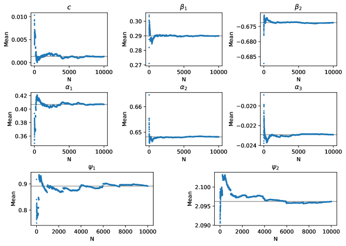
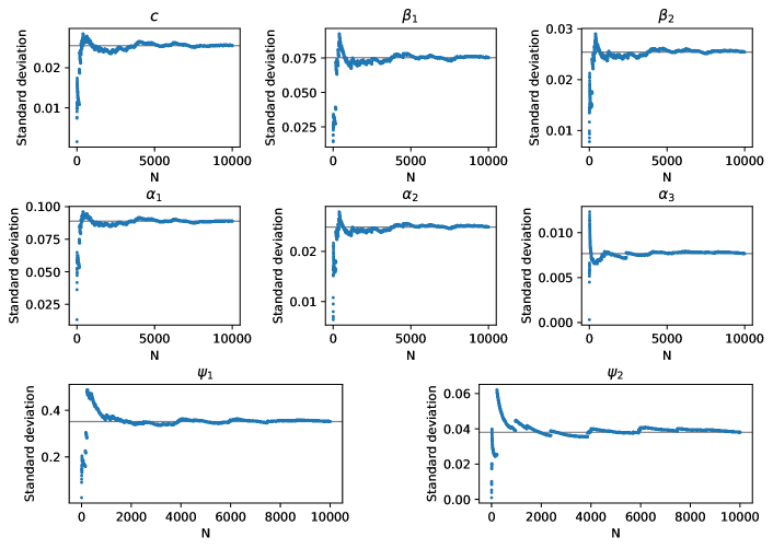
Figure 5: The mean values (top three rows) and standard deviations (bottom three rows) of the fit parameters from Eq. 2 vs. the number of samples up to $N=10,000$. The grey line indicates the final converged mean values and standard deviations after $10,000$ samples (see Table 1)

.

References

- Artigau et al. (2014) Artigau, É., Kouach, D., Donati, J.-F., et al. 2014, in Society of Photo-Optical Instrumentation Engineers (SPIE) Conference Series, Vol. 9147, Ground-based and Airborne Instrumentation for Astronomy V, ed. S. K. Ramsay, I. S. McLean, & H. Takami, 914715
- Bashi et al. (2017) Bashi, D., Helled, R., Zucker, S., & Mordasini, C. 2017, A&A, 604, A83
- Beuzit et al. (2019) Beuzit, J. L., Vigan, A., Mouillet, D., et al. 2019, A&A, 631, A155
- Bouchy et al. (2017) Bouchy, F., Doyon, R., Artigau, É., et al. 2017, The Messenger, 169, 21
- Burrows et al. (2001) Burrows, A., Hubbard, W. B., Lunine, J. I., & Liebert, J. 2001, Reviews of Modern Physics, 73, 719
- Chabrier et al. (2009) Chabrier, G., Baraffe, I., Leconte, J., Gallardo, J., & Barman, T. 2009, in American Institute of Physics Conference Series, Vol. 1094, 15th Cambridge Workshop on Cool Stars, Stellar Systems, and the Sun, ed. E. Stempels, 102–111
- Charbonneau et al. (2009) Charbonneau, D., Berta, Z. K., Irwin, J., et al. 2009, Nature, 462, 891
- Chen & Rogers (2016) Chen, H. & Rogers, L. A. 2016, ApJ, 831, 180
- Chen & Kipping (2017) Chen, J. & Kipping, D. 2017, ApJ, 834, 17
- Dorn et al. (2014) Dorn, R. J., Anglada-Escude, G., Baade, D., et al. 2014, The Messenger, 156, 7
- Dorn et al. (2023) Dorn, R. J., Bristow, P., Smoker, J. V., et al. 2023, arXiv e-prints, arXiv:2301.08048
- Edmondson et al. (2023) Edmondson, K., Norris, J., & Kerins, E. 2023, arXiv e-prints, arXiv:2310.16733
- Fortney et al. (2007) Fortney, J. J., Marley, M. S., & Barnes, J. W. 2007, ApJ, 659, 1661
- Fortney & Nettelmann (2010) Fortney, J. J. & Nettelmann, N. 2010, Space Sci. Rev., 152, 423
- Fulton et al. (2017) Fulton, B. J., Petigura, E. A., Howard, A. W., et al. 2017, AJ, 154, 109
- Gardner et al. (2006) Gardner, J. P., Mather, J. C., Clampin, M., et al. 2006, Space Sci. Rev., 123, 485
- Grasset et al. (2009) Grasset, O., Schneider, J., & Sotin, C. 2009, ApJ, 693, 722
- Guillot et al. (2006) Guillot, T., Santos, N. C., Pont, F., et al. 2006, A&A, 453, L21
- Harris et al. (2020) Harris, C. R., Millman, K. J., van der Walt, S. J., et al. 2020, Nature, 585, 357
- Hatzes & Rauer (2015) Hatzes, A. P. & Rauer, H. 2015, ApJ, 810, L25
- Helled (2023) Helled, R. 2023, A&A, 675, L8
- Helled et al. (2020) Helled, R., Mazzola, G., & Redmer, R. 2020, Nature Reviews Physics, 2, 562
- Hubbard (1977) Hubbard, W. B. 1977, Icarus, 30, 305
- Hunter (2007) Hunter, J. D. 2007, Computing in Science & Engineering, 9, 90
- Izidoro et al. (2021) Izidoro, A., Bitsch, B., Raymond, S. N., et al. 2021, A&A, 650, A152
- Izidoro et al. (2022) Izidoro, A., Schlichting, H. E., Isella, A., et al. 2022, ApJ, 939, L19
- Jontof-Hutter (2019) Jontof-Hutter, D. 2019, Annual Review of Earth and Planetary Sciences, 47, 141
- Kaeufl et al. (2004) Kaeufl, H.-U., Ballester, P., Biereichel, P., et al. 2004, in Society of Photo-Optical Instrumentation Engineers (SPIE) Conference Series, Vol. 5492, Ground-based Instrumentation for Astronomy, ed. A. F. M. Moorwood & M. Iye, 1218–1227
- Kanodia et al. (2023) Kanodia, S., He, M. Y., Ford, E. B., Ghosh, S. K., & Wolfgang, A. 2023, ApJ, 956, 76
- Kubyshkina & Fossati (2022) Kubyshkina, D. & Fossati, L. 2022, A&A, 668, A178
- Lozovsky et al. (2018) Lozovsky, M., Helled, R., Dorn, C., & Venturini, J. 2018, ApJ, 866, 49
- Malsky et al. (2023) Malsky, I., Rogers, L., Kempton, E. M. R., & Marounina, N. 2023, Nature Astronomy, 7, 57
- Mayor & Queloz (1995) Mayor, M. & Queloz, D. 1995, Nature, 378, 355
- Mordasini et al. (2012) Mordasini, C., Alibert, Y., Georgy, C., et al. 2012, A&A, 547, A112
- Mousavi-Sadr et al. (2023) Mousavi-Sadr, M., Jassur, D. M., & Gozaliasl, G. 2023, MNRAS, 525, 3469
- Muggeo (2003) Muggeo, V. M. R. 2003, Statistics in Medicine, 22, 3055
- Müller et al. (2020) Müller, S., Ben-Yami, M., & Helled, R. 2020, ApJ, 903, 147
- Müller & Helled (2023) Müller, S. & Helled, R. 2023, Frontiers in Astronomy and Space Sciences, 10, 1179000
- Otegi et al. (2020) Otegi, J. F., Bouchy, F., & Helled, R. 2020, A&A, 634, A43
- Owen & Wu (2017) Owen, J. E. & Wu, Y. 2017, ApJ, 847, 29
- Pilgrim (2021) Pilgrim, C. 2021, The Journal of Open Source Software, 6, 3859
- Quirrenbach et al. (2016) Quirrenbach, A., Amado, P. J., Caballero, J. A., et al. 2016, in Society of Photo-Optical Instrumentation Engineers (SPIE) Conference Series, Vol. 9908, Ground-based and Airborne Instrumentation for Astronomy VI, ed. C. J. Evans, L. Simard, & H. Takami, 990812
- Rauer et al. (2014) Rauer, H., Catala, C., Aerts, C., et al. 2014, Experimental Astronomy, 38, 249
- Rogers (2015) Rogers, L. A. 2015, ApJ, 801, 41
- Seager et al. (2007) Seager, S., Kuchner, M., Hier-Majumder, C. A., & Militzer, B. 2007, ApJ, 669, 1279
- Spiegel et al. (2014a) Spiegel, D. S., Fortney, J. J., & Sotin, C. 2014a, Proceedings of the National Academy of Science, 111, 12622
- Spiegel et al. (2014b) Spiegel, D. S., Fortney, J. J., & Sotin, C. 2014b, Proceedings of the National Academy of Science, 111, 12622
- Teske et al. (2019) Teske, J. K., Thorngren, D., Fortney, J. J., Hinkel, N., & Brewer, J. M. 2019, AJ, 158, 239
- The pandas development team (2020) The pandas development team. 2020, pandas-dev/pandas: Pandas
- Thorngren et al. (2016) Thorngren, D. P., Fortney, J. J., Murray-Clay, R. A., & Lopez, E. D. 2016, ApJ, 831, 64
- Tinetti et al. (2018) Tinetti, G., Drossart, P., Eccleston, P., et al. 2018, Experimental Astronomy, 46, 135
- Ulmer-Moll et al. (2019) Ulmer-Moll, S., Santos, N. C., Figueira, P., Brinchmann, J., & Faria, J. P. 2019, A&A, 630, A135
- Venturini et al. (2020) Venturini, J., Guilera, O. M., Haldemann, J., Ronco, M. P., & Mordasini, C. 2020, A&A, 643, L1
- Weiss et al. (2013) Weiss, L. M., Marcy, G. W., Rowe, J. F., et al. 2013, ApJ, 768, 14
- Wes McKinney (2010) Wes McKinney. 2010, in Proceedings of the 9th Python in Science Conference, ed. Stéfan van der Walt & Jarrod Millman, 56 – 61
- Wildi et al. (2017) Wildi, F., Blind, N., Reshetov, V., et al. 2017, in Society of Photo-Optical Instrumentation Engineers (SPIE) Conference Series, Vol. 10400, Society of Photo-Optical Instrumentation Engineers (SPIE) Conference Series, ed. S. Shaklan, 1040018
- Zeng et al. (2019) Zeng, L., Jacobsen, S. B., Sasselov, D. D., et al. 2019, Proceedings of the National Academy of Science, 116, 9723
- Zeng et al. (2016) Zeng, L., Sasselov, D. D., & Jacobsen, S. B. 2016, ApJ, 819, 127