Thermal Hall conductivity of a valence bond solid phase in the square lattice $J_{1}$-$J_{2}$ antiferromagnet Heisenberg model with a Dzyaloshinskii-Moriya interaction

Abstract

We calculate the thermal Hall conductivity $\kappa_{xy}$ for the columnar valence-bond solid phase of a two-dimensional frustrated antiferromagnet. In particular, we consider the square lattice spin-$1/2$ $J_{1}$-$J_{2}$ antiferromagnetic Heisenberg model with an additional Dzyaloshinskii-Moriya interaction between the spins and in the presence of an external magnetic field. We concentrate on the intermediate parameter region of the $J_{1}$-$J_{2}$ model, where a quantum paramagnetic phase is stable, and consider a Dzyaloshinskii-Moriya vector pattern associated with the couplings between the spins in the CuO₂ planes of the YBCO compound. We describe the columnar valence-bond solid phase within the bond-operator formalism, which allows us to map the Heisenberg model into an effective interacting boson model written in terms of triplet operators. The effective boson model is studied within the harmonic approximation and the triplon excitation bands of the columnar valence-bond solid phase is determined. We then calculate the Berry curvature and the Chern numbers of the triplon excitation bands and, finally, determine the thermal Hall conductivity due to triplons as a function of the temperature. We find that the Dzyaloshinskii-Moriya interaction yields a finite Berry curvature for the triplon bands, but the corresponding Chern numbers vanish. Although the triplon excitations are topologically trivial, the thermal Hall conductivity of the columnar valence-bond solid phase in the square lattice antiferromagnet is finite at low temperatures. We comment on the relations of our results with a no-go condition for a thermal Hall effect previously derived for ordered magnets.

I Introduction

The topological properties of the elementary excitations of insulating quantum magnets [1, 2] have been receiving some attention in recent years [3, 4]. Long-range ordered phases in ferromagnets [5, 6, 7, 8, 9, 10] and in antiferromagnets (AFMs) [11, 12, 13] with topologically nontrivial magnon excitations, in addition to valence bond solid (VBS) phases in AFMs [14, 15, 16, 17] with topologically nontrivial triplon excitations have been reported. Such systems, whose excitations bands have nonzero Chern numbers, are the bosonic analogues of the Chern band insulators: noninteracting fermionic systems whose electronic bands are characterized by a finite Chern number [18, 19, 20].

Experimentally, the nontrivial topological properties of insulating quantum magnets can be probed, for instance, via measurements of the thermal Hall conductivity $\kappa_{xy}$ [21, 22, 23]. Differently from Chern band insulators, whose nontrivial topological properties yield an anomalous quantum Hall effect (a quantized Hall conductance in the absence of an external magnetic field) [24], magnons and triplons are charge-neutral excitations, and therefore, do not respond to an applied electric field [4]. However, in the presence of a temperature gradient, magnons and triplons may induce a transverse (Hall) heat current, in addition to the (usual) longitudinal one. Indeed, a magnon thermal Hall effect has been described in ferromagnets on honeycomb [6, 8, 9], Shastry-Sutherland [7], pyrochlore [23, 25], and perovskite [25] lattices, and in AFMs on kagome [12], honeycomb [13], and square [26] lattices, while a triplon thermal Hall effect has been predicted for the Shastry-Sutherland compound SrCu₂(BO₃)₂ [14, 15]. One should also mention the spin Nernst effect of magnons (the analogue of the spin Hall effect for electrons) in AFMs on a honeycomb lattice [27, 11] and a thermal Hall effect due to bosonic spinons [28, 29] in spin liquid phases. Interestingly, although a serie of studies has been devoted to the magnon thermal Hall effect in insulating quantum magnets, the triplon thermal Hall effect has received few attention.

                             

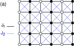
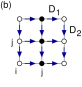
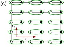
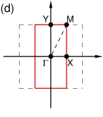
Figure 1: Schematic representations: (a) The square lattice spin-$1/2$ $J_{1}$-$J_{2}$ AFM Heisenberg model (2). (b) The DM vectors ${\bf D}_{ij}$ [Eq. (3)] for the spins in the CuO₂ planes of the YBCO compound; ${\bf D}_{1}=(D,0,0)$ and ${\bf D}_{2}=(0,-D,0)$. (c) The columnar VBS ground state; the green ellipses indicate that the spins ${\bf S}^{1}$ (open circle) and ${\bf S}^{2}$ (filled circle) form a singlet state; $\mbox{\boldmath$\tau$}_{1}$ and $\mbox{\boldmath$\tau$}_{2}$ [Eq. (11)] are the primitive vectors of the dimerized lattice $\mathcal{D}$ defined by the (green) singlets. (d) Brillouin zones of the dimerized (solid red line) and the original square (dashed black line) lattices; $\mathbf{X}=(\pi/2,0)$, $\mathbf{M}=(\pi/2,\pi)$, and $\mathbf{Y}=(0,\pi)$ with the lattice spacing $a$ of the original square lattice being set to 1.

The magnon thermal Hall effect in insulating quantum magnets was theoretically studied in Refs. [21, 22, 23]. Based on linear spin-wave theory results, Katsura et al. [21] show that the lattice geometry may constraint the presence or absence of a thermal Hall effect, namely, the thermal Hall conductivity should vanish (a no-go theorem) in quantum magnets whose unit cells share edges, such as the ones realized in triangular and square lattices. Moreover, starting from a Kubo formula, it was shown that the thermal Hall conductivity is finite for a ferromagnet on a (corner sharing) kagome lattice [21]. Performing a semiclassical analysis and using liner response theory, Matsumoto and Murakami [22, 23] determine the thermal transport coefficients for a long-range magnetic ordered phase in a ferromagnet and show that the thermal Hall conductivity $\kappa_{xy}$ can be written in terms of the Berry curvatures of the magnon excitation bands. It was verify that [5, 6, 30, 8, 7, 25, 10, 27, 11, 26, 14, 15, 16, 17, 31] one important ingredient that may yield a finite Berry curvature for the bosonic (magnon and triplon) excitation bands is the Dzyaloshinskii-Moriya (DM) interaction [32, 33, 34], an interaction between localized spins which is associated with the spin-orbit coupling, and therefore, acts as a kind of pseudomagnetic field for magnons and triplons. It should be mentioned that the formalism [22, 23] is indeed quite general, such that the expression derived for the thermal Hall conductivity $\kappa_{xy}$ can be applied to any quantum magnet with bosonic elementary excitations.

In this paper, we study the triplon thermal Hall effect, in particular, we calculate the thermal Hall conductivity $\kappa_{xy}$ for a VBS phase realized in a square-lattice frustrated AFM. We consider the spin-$1/2$ $J_{1}$-$J_{2}$ AFM Heisenberg model on a square lattice [Fig. 1(a)], with an additional DM interaction between the nearest-neighbor spins [Fig. 1(b)] and in the presence of an external magnetic field. We focus on the intermediate parameter region $0.4\,J_{1}\lesssim J_{2}\lesssim 0.6\,J_{1}$ of the $J_{1}$-$J_{2}$ model, where a quantum paramagnetic phase sets in, and, in particular, consider the columnar VBS phase [Fig. 1(c)]. The main purpose of this paper is to verify whether a DM interaction in the square-lattice AFM yields a columnar VBS phase with topologically nontrivial triplon excitations and whether the no-go theorem for the thermal Hall effect derived in Ref. [21] for an ordered magnet also applies for a quantum paramagnetic phase, in particular, a VBS phase.

I.1 Overview of the results

We study a spin-$1/2$ frustrated AFM on a square lattice with the aid of the bond-operator formalism [35]. We show that the columnar VBS phase can be described by an effective interacting boson model expressed in terms of triplet operators. We consider the effective boson model in the (lowest-order) harmonic approximation and determine the triplon excitation bands. Moreover, we calculate the Berry curvatures and Chern numbers of the triplon bands. Following the lines of the formalism [22, 23], which was previously applied in the study of the magnon thermal Hall effect, we finally determine the thermal Hall conductivity $\kappa_{xy}$ due to the triplons as a function of the temperature. We find that the Berry curvature of the triplon bands are finite in some regions of the first (dimerized) Brillouin zone, but the triplons are topologically trivial, since the Chern numbers of the triplon bands vanish. Our main find is indeed the determination of the dependence of the thermal Hall conductivity $\kappa_{xy}$ with the temperature $T$: In spite of the fact that the triplon excitations are topologically trivial, $\kappa_{xy}$ is finite at low temperatures; such a result agrees with Ref. [29], where $\kappa_{xy}$ is determined for a spin liquid phase realized in a two-dimensional AFM whose Heisenberg model includes the same DM interaction considered in our paper, but it is in disagreement with the no-go condition [21] for a thermal Hall effect due to magnons, previously determined for long-range ordered magnets.

I.2 Outline

Our paper is organized as follows. In Sec. II, we introduce the Hamiltonian of the spin-$1/2$ frustrated AFM Heisenberg model on a square lattice considered in our study. In Sec. III, we briefly review the bond-operator representation [35] for spin operators, a formalism which allows us to describe the columnar VBS phase, and derive an effective interacting boson model in terms of triplet operators. The effective boson model is analysed within the harmonic approximation in Sec. IV and the region of stability of the columnar VBS phase and the energy of the elementary triplon excitations are determined. Sec. V is devoted to the calculation of the Berry curvatures of the triplon excitation bands and the determination of the corresponding Chern numbers. The thermal Hall conductivity $\kappa_{xy}$ for the columnar VBS phase is discussed in Sec. VI. Finally, a brief summary of our main findings are provided in the Sec. VII. Some further details about the effective boson model and the analytical procedure employed in the diagonalization of the effective boson model within the harmonic approximation can be found in the three Appendices.

II Frustrated square-lattice antiferromagnet

Let us consider a frustrated spin-$1/2$ Heisenberg AFM on a square lattice described by the Hamiltonian

$$\mathcal{H}=\mathcal{H}_{J}+\mathcal{H}_{\rm DM}+\mathcal{H}_{B},$$ (1)

where $\mathcal{H}_{J}$ is the Hamiltonian of the $J_{1}$-$J_{2}$ square-lattice AFM Heisenberg model,

$$\mathcal{H}_{J}=J_{1}\sum_{\langle ij\rangle}{\bf S}_{i}\cdot{\bf S}_{j}+J_{2}\sum_{\langle\langle ij\rangle\rangle}{\bf S}_{i}\cdot{\bf S}_{j},$$ (2)

$\mathcal{H}_{\rm DM}$ is the DM interaction term [32, 33, 34],

$$\mathcal{H}_{\rm DM}=\sum_{\langle ij\rangle}{\bf D}_{ij}\cdot\left({\bf S}_{i}\times{\bf S}_{j}\right),$$ (3)

and $\mathcal{H}_{B}$ is the Zeeman term that describes the coupling of the spins with an external magnetic field ${\bf B}$,

$$\mathcal{H}_{B}=-g\mu_{B}{\bf B}\cdot\sum_{i}{\bf S}_{i}\equiv-{\bf h}\cdot\sum_{i}{\bf S}_{i}.$$ (4)

Here ${\bf S}_{i}$ is a spin-$1/2$ operator at site $i$ and $J_{1}>0$ and $J_{2}>0$ are, respectively, the nearest-neighbor and next-nearest-neighbor exchange couplings as illustrated in Fig. 1(a). ${\bf D}_{ij}$ is a DM vector that couples the spins ${\bf S}_{i}$ and ${\bf S}_{j}$; we consider, in particular, the DM vector pattern shown in Fig. 1(b), which corresponds to the symmetry-allowed couplings between the spins in the CuO₂ planes of the YBCO compound [36, 37, 38]. Finally, $g$ is the electron g factor and $\mu_{B}$ the Bohr magneton. It should be mentioned that the AFM Heisenberg model (1), without the next-nearest-neighbor exchange coupling $J_{2}$ and an additional symmetric pseudodipolar interaction between the spins ($\Gamma$ term), was previously considered in the study of the cuprate superconductors, as discussed, e.g., in Refs. [39, 40, 41].

The $J_{1}$-$J_{2}$ model (2) has been receiving a lot of attention in the last few years and now its phase diagram at temperature $T=0$ is well established [42, 43, 44, 45, 35, 46, 47, 48, 49, 50, 51, 52, 53, 54, 55, 56, 57, 58, 59, 60, 61, 62, 63, 64, 65, 66, 67, 68, 69, 70, 71, 72, 73, 74, 75, 76, 77, 78, 79, 80, 81, 82, 83, 84, 85, 86, 87, 88, 89, 90, 91, 92, 93, 94, 95, 96, 97, 98, 99]: A semiclassical Néel long-range ordered phase with ordering wave vector ${\bf Q}=(\pi,\pi)$ sets in for $J_{2}\lesssim 0.4\,J_{1}$, a quantum paramagnetic phase is stable in the intermediate parameter region $0.4\,J_{1}\lesssim J_{2}\lesssim 0.6\,J_{1}$, and a stripe long-range ordered phase with ${\bf Q}=(\pi,0)$ or $(0,\pi)$ is the ground state for $J_{2}\gtrsim 0.6\,J_{1}$. Interestingly, the nature of the quantum paramagnetic phase is still an open issue. Among the several proposals that have been made for the ground state of the model (2) within this intermediate parameter region, one should mention: The (dimerized) columnar [55, 56, 86] and staggered [79] VBSs, where both translational and rotational lattice symmetries are broken; the (tetramerized) plaquette VBS, where only the translational lattice symmetry is broken [54, 57, 59, 61, 68, 71, 80, 81]; a mixed columnar-plaquette VBS [67]; gapless [58, 60, 75, 76, 82, 87, 88] and gapped [72, 73, 74, 85] spin-liquid ground states. More recently, it was found that, within the intermediate parameter region, a gapless spin-liquid phase sets in for $J_{2}\lesssim 0.53J_{1}$ while a VBS is stable for $J_{2}\gtrsim 0.53J_{1}$ [83, 89, 94, 95, 97]; such results qualitatively agree with previous density matrix renormalization group (DMRG) calculations [81], which indicate a gapless phase for $0.44\,J_{1}<J_{2}<0.50\,J_{1}$ and a VBS one for $0.50\,J_{1}<J_{2}<0.61\,J_{1}$, although with a plaquette singlet pattern.

Although the $J_{1}$-$J_{2}$ model (2) has been extensively studied, few attention has been devoted to the description of the effects of an additional (anisotropic) DM interaction between the spins. Exact diagonalization results [100] for the Heisenberg model (1), without an external magnetic field, found that the extension of the quantum paramagnetic region of the $J_{1}$-$J_{2}$ model (2) is affected by the presence of a finite DM interaction. More recently, a Majorana fermion representation for the spin operators was employed in order to describe a chiral spin-liquid phase of the model (1) [101]: based on a mean-field approach, the stability of such a spin-liquid phase was studied; exact diagonalization results were also reported. In both studies [100] and [101], DM vectors associated with cuprate superconductor compounds were considered.

In the following, we consider the AFM Heisenberg model (1) within the intermediate parameter region $0.4\,J_{1}\lesssim J_{2}\lesssim 0.6\,J_{1}$ for the next-nearest neighbor exchange coupling $J_{2}$ and DM interaction $D\leq 0.50\,J_{1}$, where

$$D=|{\bf D}_{1}|=|{\bf D}_{2}|,$$ (5)

see Fig. 1(b). In particular, we concentrate on the columnar VBS phase illustrated in Fig. 1(c). Indeed, the region of stability of the columnar VBS phase for the $J_{1}$-$J_{2}$ model (2) and the spectrum of the elementary (triplon) excitations were determined by one of us within the bond-operator formalism in Ref. [93].

III Bond operator Formalism

The bond-operator representation for spin operators introduced by Sachdev and Bhatt [35] is a formalism that allows us to describe a dimerized VBS phase. In this section, this formalism is briefly summarized, following the lines of Refs. [102, 93].

Let us consider the Hilbert space of two $S=1/2$ spins, ${\bf S}^{1}$ and ${\bf S}^{2}$, which is made out of a singlet $|s\rangle$ and three triplet $|t_{\alpha}\rangle$ states:

$$|s\rangle = \frac{1}{\sqrt{2}}\left(|\uparrow\downarrow\rangle-|\downarrow\uparrow\rangle\right),\;\;\;\;\;\;\;|t_{x}\rangle=\frac{1}{\sqrt{2}}\left(|\downarrow\downarrow\rangle-|\uparrow\uparrow\rangle\right),$$

$$|t_{y}\rangle = \frac{i}{\sqrt{2}}\left(|\uparrow\uparrow\rangle+|\downarrow\downarrow\rangle\right),\;\;\;\;\;\;\;|t_{z}\rangle=\frac{1}{\sqrt{2}}\left(|\uparrow\downarrow\rangle+|\downarrow\uparrow\rangle\right).$$

Let us define a set of boson operators, $s^{\dagger}$ and $t^{\dagger}_{\alpha}$, with $\alpha=x$, $y$, $z$, which respectively creates the singlet and the three triplet states out of a fictitious vacuum $|0\rangle$,

$$|s\rangle=s^{\dagger}|0\rangle\;\;\;\;\;\;{\rm and}\;\;\;\;\;\;|t_{\alpha}\rangle=t_{\alpha}^{\dagger}|0\rangle.$$ (7)

In order to remove unphysical states from the enlarged Hilbert space, one should introduce the constraint

$$s^{\dagger}s+\sum_{\alpha}t^{\dagger}_{\alpha}t_{\alpha}=1.$$ (8)

One then calculates the matrix elements of each component of the spin operators ${\bf S}^{1}$ and ${\bf S}^{2}$ within the basis $|s\rangle$ and $|t_{\alpha}\rangle$, i.e., one determines $\langle s|S^{\mu}_{\alpha}|s\rangle$, $\langle s|S^{\mu}_{\alpha}|t_{\beta}\rangle$, and $\langle t_{\gamma}|S^{\mu}_{\alpha}|t_{\beta}\rangle$, with $\mu=1$, $2$ and $\alpha$, $\beta$, $\gamma=$ $x$, $y$, $z$. Based on the set of obtained results, one easily concludes that the components of the spin operators ${\bf S}^{1}$ and ${\bf S}^{2}$ can be expanded in terms of the boson operators $s^{\dagger}$ and $t^{\dagger}_{\alpha}$ as

$$S^{1,2}_{\alpha}=\pm\frac{1}{2}\left(s^{\dagger}t_{\alpha}+t^{\dagger}_{\alpha}s\mp i\epsilon_{\alpha\beta\gamma}t^{\dagger}_{\beta}t_{\gamma}\right),$$ (9)

where $\epsilon_{\alpha\beta\gamma}$ is the completely antisymmetric tensor with $\epsilon_{xyz}=1$ and the summation convention over repeated indices is assumed. Adding a site index $i$ to the singlet and triplet operators, i.e., defining the boson operators $s^{\dagger}_{i}$ and $t^{\dagger}_{i\,\alpha}$, one generalizes the bond-operator representation (9) for spin operators ${\bf S}_{i}$ on a given lattice.

One should mention that a generalization of the bond-operator representation (9) for a tetramerized (plaquette) VBS, which includes two singlet, nine triplet, and five quintet boson operators, was introduced by one of us in Ref. [80].

III.1 Effective boson model

With the aid of the generalized bond-operator representation (9), we now map the AFM Heisenberg model (1) into an effective boson model that is written in terms of the triplet operators $t_{i\,\alpha}$. Such an effective model allows us to describe the corresponding columnar VBS phase. In order to perform the mapping, one needs to express the Hamiltonian (1) in terms of the underline dimerized lattice $\mathcal{D}$, which is defined by the singlet (dimer) arrangement of the columnar VBS state, see Fig. 1(c).

Let us first consider the $J_{1}$-$J_{2}$ model (2). In terms of the underline dimerized lattice $\mathcal{D}$, the Hamiltonian (2) assumes the form

$$\mathcal{H}_{J}= \sum_{i\in\mathcal{D}}J_{1}\left({\bf S}^{1}_{i}\cdot{\bf S}^{2}_{i}+{\bf S}^{1}_{i}\cdot{\bf S}^{1}_{i+2}+{\bf S}^{2}_{i}\cdot{\bf S}^{2}_{i+2}+{\bf S}^{2}_{i}\cdot{\bf S}^{1}_{i+1}\right)$$

$$+J_{2}\left({\bf S}^{1}_{i}\cdot{\bf S}^{2}_{i+2}+{\bf S}^{2}_{i}\cdot{\bf S}^{1}_{i+2}\right)$$

$$+J_{2}\left({\bf S}^{2}_{i}\cdot{\bf S}^{1}_{i+1+2}+{\bf S}^{2}_{i}\cdot{\bf S}^{1}_{i+1-2}\right),$$ (10)

where $i$ is a site of the dimerized lattice $\mathcal{D}$, ${\bf S}^{1}_{i}$ and ${\bf S}^{2}_{i}$ are the two spins within each unit cell, and the (lower) index $n=1,2$ indicates the dimer nearest-neighbor vectors $\mbox{\boldmath$\tau$}_{n}$,

$$\mbox{\boldmath$\tau$}_{1}=2a\hat{x},\;\;\;\;\;\;\;\;\;\;\;\mbox{\boldmath$\tau$}_{2}=a\hat{y},$$ (11)

with $a$ being the lattice spacing of the original square lattice, see Fig. 1(c). In the following, we set $a=1$. Substituting the generalized bond-operator representation (9) into the Hamiltonian (10), one finds that [93]

$$\mathcal{H}_{J}=\mathcal{H}_{J,0}+\mathcal{H}_{J,2}+\mathcal{H}_{J,3}+\mathcal{H}_{J,4},$$ (12)

where each $\mathcal{H}_{J,n}$ term has $n$ triplet operators as shown in Eq. (LABEL:h-boson1ap). Finally, the constraint (8) is treated on average via a Lagrange multiplier $\mu$: one then adds the following term to the Hamiltonian (12)

$$-\mu\sum_{i}\left(s_{i}^{\dagger}s_{i}+t_{i\alpha}^{\dagger}t_{i\alpha}-1\right).$$

In the bond-operator formalism, a dimerized VBS ground state, such as the columnar VBS one, can be viewed as a condensate of the singlets $s_{i}$. One then sets

$$s_{i}^{\dagger}=s_{i}=\langle s_{i}^{\dagger}\rangle=\langle s_{i}\rangle\rightarrow\sqrt{N_{0}}$$ (13)

in the Hamiltonian (12) and, therefore, arrives at an effective boson model expressed only in terms of the triplet boson operators $t_{i\alpha}$. As discussed in Sec. IV below, the constants $N_{0}$ and $\mu$ are self-consistently calculated for fixed values of the next-nearest-neighbor exchange coupling $J_{2}$, the DM interaction $D$, and the external magnetic field $h$.

It is useful to write the Hamiltonian (12) in momentum space. Considering the Fourier transform of the triplet operators $t_{i\alpha}$,

$$t_{i\alpha}=\frac{1}{\sqrt{N^{\prime}}}\sum_{{\bf k}\in{\rm BZ}}e^{i{\bf k}\cdot{\bf R}_{i}}\>t_{{\bf k}\alpha},$$ (14)

with ${\bf R}_{i}$ being a vector of the dimerized lattice $\mathcal{D}$, $N^{\prime}=N/2$ the number of dimers ($N$ is the number of sites of the original square lattice), and the momentum sum running over the (dimerized) first Brillouin zone [see Fig. 1(d)], one shows that the four terms $\mathcal{H}_{J,n}$ of the Hamiltonian (12) assume the form

$$\mathcal{H}_{J,0} =-\frac{3}{8}J_{1}NN_{0}-\frac{1}{2}\mu N(N_{0}-1),$$ (15)

$$\mathcal{H}_{J,2} =\sum_{\bf k}\left[A_{\bf k}t^{\dagger}_{{\bf k}\alpha}t_{{\bf k}\alpha}+\frac{1}{2}B_{\bf k}\left(t^{\dagger}_{{\bf k}\alpha}t^{\dagger}_{-{\bf k}\alpha}+{\rm H.c.}\right)\right],$$ (16)

$$\mathcal{H}_{J,3} =\frac{1}{2\sqrt{N^{\prime}}}\epsilon_{\alpha\beta\lambda}\sum_{{\bf p},{\bf k}}\xi_{{\bf k}-{\bf p}}\;t^{\dagger}_{{\bf k}-{\bf p}\alpha}t^{\dagger}_{{\bf p}\beta}t_{{\bf k}\lambda}+{\rm H.c.},$$ (17)

$$\mathcal{H}_{J,4} =\frac{1}{2N^{\prime}}\epsilon_{\alpha\beta\lambda}\epsilon_{\alpha\mu\nu}\sum_{{\bf q},{\bf p},{\bf k}}\gamma_{\bf k}\;t^{\dagger}_{{\bf p}+{\bf k}\beta}t^{\dagger}_{{\bf q}-{\bf k}\mu}t_{{\bf q}\nu}t_{{\bf p}\lambda},$$ (18)

with the coefficients $A_{\bf k}$, $B_{\bf k}$, $\xi_{\bf k}$, and $\gamma_{\bf k}$ given by

$$A_{\bf k}= \frac{1}{4}J_{1}-\mu+B_{\bf k},$$

$$B_{\bf k}= -\frac{1}{2}N_{0}\left[J_{1}\cos(2k_{x})-2(J_{1}-J_{2})\cos(k_{y})\right.$$

$$+\left.J_{2}\cos(2k_{x}+k_{y})+J_{2}\cos(2k_{x}-k_{y})\right],$$

$$\xi_{\bf k}= -\sqrt{N_{0}}\left[J_{1}\sin(2k_{x})+J_{2}\sin(2k_{x}+k_{y})\right.$$

$$+\left.J_{2}\sin(2k_{x}-k_{y})\right],$$

$$\gamma_{\bf k}= -\frac{1}{2}\left[J_{1}\cos(2k_{x})+2(J_{1}+J_{2})\cos k_{y}\right.$$

$$+\left.J_{2}\cos(2k_{x}+k_{y})+J_{2}\cos(2k_{x}-k_{y})\right].$$

We should mention that the effective boson model (12) was previously derived by one of us in Ref. [93]. For completeness, we provide here all the details of the procedure that, in the following, will be applied to the DM term (3) and the Zeeman coupling (4).

In terms of the sites $i$ of the underline dimerized lattice $\mathcal{D}$, the DM interaction (3) reads

$$\mathcal{H}_{\rm DM}=\sum_{i\in\mathcal{D}} \Big{[}{\bf D}_{i,i}\cdot({\bf S}_{i}^{1}\times{\bf S}_{i}^{2})+{\bf D}_{i,i+1}\cdot({\bf S}_{i}^{2}\times{\bf S}_{i+1}^{1})\Big{.}$$

$$+\Big{.}{\bf D}_{i,i+2}\cdot({\bf S}_{i}^{2}\times{\bf S}_{i+2}^{2})\Big{.}$$

$$+\Big{.}{\bf D}_{i,i+2}\cdot({\bf S}_{i}^{1}\times{\bf S}_{i+2}^{1})\Big{]},$$ (20)

where the DM vectors ${\bf D}_{i,j}$ are given by [see Fig. 1(b)]

$${\bf D}_{i,i}={\bf D}_{i,i+1}={\bf D}_{1}=(D,0,0),$$

$${\bf D}_{i,i+2}={\bf D}_{2}=(0,-D,0).$$ (21)

Again, substituting the bond-operator representation (9) generalized to the lattice case into the Hamiltonian (20), we show that

$$\mathcal{H}_{\rm DM}=\mathcal{H}_{\rm DM,1}+\mathcal{H}_{\rm DM,2}+\mathcal{H}_{\rm DM,3}+\mathcal{H}_{\rm DM,4},$$ (22)

where the $\mathcal{H}_{\rm DM,n}$ term contains $n$ triplet operators, see Eq. (LABEL:h-boson2ap) for details. After replacing the singlet operators by its average value (13), we performe a Fourier transform with the aid of Eq. (14) and find the expressions of the $\mathcal{H}_{\rm DM,n}$ terms in momentum space, namely,

$$\mathcal{H}_{\rm DM,2}= -i\sum_{\bf k}\Big{[}\Big{(}C_{\bf k}\,\epsilon_{y\beta\gamma}+D_{\bf k}\,\epsilon_{x\beta\gamma}\Big{)}t^{\dagger}_{{\bf k}\beta}t_{{\bf k}\gamma}\Big{.}$$

$$+\Big{.}\frac{1}{2}C_{\bf k}\,\epsilon_{y\beta\gamma}\left(t_{-{\bf k}\beta}t_{{\bf k}\gamma}-t^{\dagger}_{{\bf k}\gamma}t^{\dagger}_{-{\bf k}\beta}\right)\Big{.}$$

$$+\Big{.}\frac{1}{2}D_{\bf k}\,\epsilon_{x\beta\gamma}\left(t_{-{\bf k}\beta}t_{{\bf k}\gamma}-t^{\dagger}_{{\bf k}\gamma}t^{\dagger}_{-{\bf k}\beta}\right)\Big{]},$$ (23)

$$\mathcal{H}_{\rm DM,3}= +i\frac{1}{2\sqrt{N^{\prime}}}\epsilon_{x\beta\gamma}\epsilon_{\gamma\mu\nu}\sum_{{\bf k},{\bf p}}\xi^{\rm DM}_{{\bf k}-{\bf p}}\,\times$$

$$\times\left(t^{\dagger}_{{\bf k}-{\bf p}\beta}t^{\dagger}_{{\bf p}\mu}t_{{\bf k}\nu}-t^{\dagger}_{{\bf k}\nu}t_{{\bf k}-{\bf p}\beta}t_{{\bf p}\mu}\right),$$ (24)

$$\mathcal{H}_{\rm DM,4}= -i\frac{1}{2N^{\prime}}\epsilon_{\beta\mu\nu}\epsilon_{\lambda\mu^{\prime}\nu^{\prime}}\sum_{\bf k}\Big{(}\epsilon_{x\beta\lambda}\,\gamma^{\rm DM}_{x,{\bf k}}\Big{.}$$

$$-\Big{.}\epsilon_{y\beta\lambda}\,\gamma^{\rm DM}_{y,{\bf k}}\Big{)}t^{\dagger}_{{\bf p}+{\bf k}\mu}t^{\dagger}_{{\bf q}-{\bf k}\mu^{\prime}}t_{{\bf p}\nu}t_{{\bf q}\nu^{\prime}},$$ (25)

where the coefficients $C_{\bf k}$, $D_{\bf k}$, $\xi^{\rm DM}_{\bf k}$, and $\gamma^{\rm DM}_{\alpha,{\bf k}}$ are defined as

$$C_{\bf k}= DN_{0}\sin(k_{y}),\quad\quad\quad D_{\bf k}=\frac{1}{2}DN_{0}\sin(2k_{x}),$$

$$\xi^{\rm DM}_{\bf k}= D\sqrt{N_{0}}\cos\left(2k_{x}\right),$$ (26)

$$\gamma^{\rm DM}_{\alpha,{\bf k}}= D\left(\frac{1}{2}\delta_{\alpha,x}\sin\left(2k_{x}\right)+\delta_{\alpha,y}\sin k_{y}\right).$$

A few remaks here about the linear term $\mathcal{H}_{\rm DM,1}$ are in order: The linear term couples the singlet $s_{i}$ and the triplet $t_{ix}$ operators, see Eq. (LABEL:h-boson2ap); it can be removed via an unitary transformation performed in each site of the dimerized lattice $\mathcal{D}$; we follow the lines of Ref. [16] and consider an unitary transformation up to first order in the parameter $\alpha=D/(2J_{1})$; as described in details in Appendix B, one of the effects of such an unitary transformation is to modify the coefficient $D_{\bf k}$ of the quadratic Hamiltonian $\mathcal{H}_{\rm DM,2}$, namely, $D_{\bf k}\rightarrow D_{\bf k}+D^{\prime}_{\bf k}$, with $D^{\prime}_{\bf k}$ given by Eq. (63); the new coefficient $D_{\bf k}$ (the one considered in Sec. IV below) then reads

$$D_{\bf k}= DN_{0}\sin(2k_{x})+\frac{1}{2}DN_{0}\frac{J_{2}}{J_{1}}\left[\sin\left(2k_{x}+k_{y}\right)\right.$$

$$\left.+\sin\left(2k_{x}-k_{y}\right)\right].$$ (27)

Finally, one easily rewrites the Zeeman coupling (4) in terms of the dimerized lattice $\mathcal{D}$:

$$\mathcal{H}_{B}=-\sum_{i\in\mathcal{D}}h_{\alpha}\left({\bf S}^{1}_{i\alpha}+{\bf S}^{2}_{i\alpha}\right).$$ (28)

With the aid of Eq. (9), one finds the expansion of the Hamiltonian (28) in terms of the triplet operators $t_{i\alpha}$ [see Eq. (55)] and, after the Fourier transform (14), shows that

$$\mathcal{H}_{B}=i\epsilon_{\alpha\beta\gamma}\sum_{\bf k}h_{\alpha}\,t_{{\bf k}\beta}^{\dagger}t_{{\bf k}\gamma},$$ (29)

where $h_{\alpha}$, with $\alpha=x,y,z$, is the $\alpha$-component of the external magnetic field ${\bf h}=g\mu_{B}{\bf B}$.

IV Harmonic approximation

In this section, the effective boson model defined by the Hamiltonians (12), (22), and (29) is studied in the lowest-order (harmonic) approximation. In this case, only terms up to quadratic order in the triplet operators $t_{{\bf k}\alpha}$ are retained, i.e., one considers

$$\mathcal{H}\approx\mathcal{H}_{J,0}+\mathcal{H}_{J,2}+\mathcal{H}_{\rm DM,2}+\mathcal{H}_{B}.$$ (30)

         

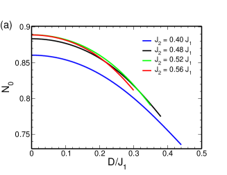
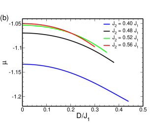
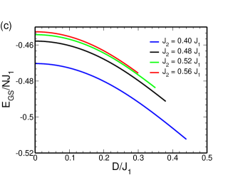
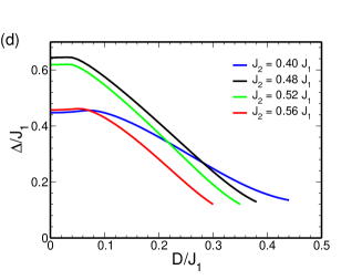
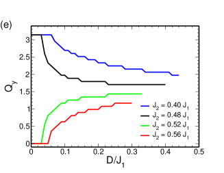
Figure 2: Parameters (a) $N_{0}$ and (b) $\mu$, (c) the ground-state energy $E_{GS}/(NJ_{1})$, (d) the triplon gap $\Delta/J_{1}$, and (e) the $y$-component $Q_{y}$ of the momentum ${\bf Q}=(0,Q_{y})$ associated with the triplon gap as functions of the DM interaction $D/J_{1}$ for the columnar VBS ground state (harmonic approximation). Next-nearest-neighbor exchange couplings $J_{2}=0.40\,J_{1}$ (blue line), $J_{2}=0.48\,J_{1}$ (black line), $J_{2}=0.52\,J_{1}$ (green line), and $J_{2}=0.56\,J_{1}$ (blue line) and the external magnetic field $h_{z}=0.05\,J_{1}$.

In order to diagonalize the quadratic Hamiltonian (30), it is useful to rewrite it in matrix form,

$$\mathcal{H}=E_{0}+\frac{1}{2}\sum_{\bf k}\Psi_{\bf k}^{\dagger}\hat{H}_{\bf k}\Psi_{\bf k},$$ (31)

where

$$E_{0}=\mathcal{H}_{J,0}-\frac{3}{2}\sum_{\bf k}A_{\bf k}$$ (32)

is a constant,

$$\Psi_{\bf k}^{\dagger}=\begin{pmatrix}t_{{\bf k},x}^{\dagger}&t_{{\bf k},y}^{\dagger}&t_{{\bf k},z}^{\dagger}&t_{-{\bf k},x}&t_{-{\bf k},y}&t_{-{\bf k},z}\end{pmatrix}$$ (33)

is a six-component vector, and

$$\hat{H}_{\bf k}=\begin{pmatrix}\hat{A}_{\bf k}+\hat{H}_{B}&\hat{B}_{\bf k}\\ \hat{B}_{\bf k}&\hat{A}_{\bf k}-\hat{H}_{B}\end{pmatrix}$$ (34)

is a $6\times 6$ matrix with the $3\times 3$ matrices $\hat{A}_{\bf k}$, $\hat{B}_{\bf k}$, and $\hat{H}_{B}$ defined as

$$\hat{A}_{\bf k} =\begin{pmatrix}A_{\bf k}&0&iC_{\bf k}\\ 0&A_{\bf k}&-iD_{\bf k}\\ -iC_{\bf k}&iD_{\bf k}&A_{\bf k}\end{pmatrix},$$

$$\hat{B}_{\bf k} =\begin{pmatrix}B_{\bf k}&0&iC_{\bf k}\\ 0&B_{\bf k}&-iD_{\bf k}\\ -iC_{\bf k}&iD_{\bf k}&B_{\bf k}\end{pmatrix},$$ (35)

$$\hat{H}_{B} =\begin{pmatrix}0&ih_{z}&-ih_{y}\\ -ih_{z}&0&ih_{x}\\ ih_{y}&-ih_{x}&0\end{pmatrix}.$$

Here, the coefficients $A_{\bf k}$ and $B_{\bf k}$ are given by Eq. (LABEL:coefs01) while the coefficients $C_{\bf k}$ and $D_{\bf k}$ are, respectively, given by Eqs. (26) and (27); as mentioned in the previous section and discussed in Appendix B, the expression (27) for the coefficient $D_{\bf k}$ includes the effects of the linear term $\mathcal{H}_{\rm DM,1}$ [Eq. (LABEL:h-boson2ap)] associated with the DM interaction (3). Finally, $h_{\alpha}=g\mu_{B}B_{\alpha}$, with $\alpha=x,y,z$, are the components of the external magnetic field; in the following, we assume that ${\bf B}=B\hat{z}$.

The diagonalization of the $6\times 6$ problem defined by Eqs. (31)–(34) is rather involved. It is then interesting to employ the procedure described in Refs. [103, 104]: Since we are dealing with a bosonic Hamiltonian, instead of the matrix (34), we should diagonalize

$$\hat{I}_{B}\hat{H}_{\bf k}\quad\quad{\rm with}\quad\quad\hat{I}_{B}=\begin{pmatrix}\hat{I}&0\\ 0&-\hat{I}\end{pmatrix}$$ (36)

and $\hat{I}$ being the $3\times 3$ identity matrix. The positive eigenvalues $\omega^{\alpha}_{\bf k}$ of the matrix (36), with $\alpha=x,y,z$, are indeed the roots of a cubic polynomial and are shown in Appendix C, see Eq. (66). After the diagonalization, the Hamiltonian (31) assumes the form

$$\mathcal{H}=E_{GS}+\frac{1}{2}\sum_{\bf k}\Phi_{\bf k}^{\dagger}\hat{H}^{\prime}_{\bf k}\Phi_{\bf k},$$ (37)

where

$$E_{GS}=-\frac{3}{8}J_{1}N_{0}N-\frac{1}{2}\mu N(N_{0}-1)+\frac{1}{2}\sum_{{\bf k},\alpha}\left(\omega_{\bf k}^{\alpha}-A_{\bf k}\right)$$ (38)

is the ground-state energy,

$$\Phi_{\bf k}^{\dagger}=\begin{pmatrix}b_{{\bf k},x}^{\dagger}&b_{{\bf k},y}^{\dagger}&b_{{\bf k},z}^{\dagger}&b_{-{\bf k},x}&b_{-{\bf k},y}&b_{-{\bf k},x}\end{pmatrix}$$ (39)

is a six-component vector whose components are the new boson (triplon) operators $b_{{\bf k},\alpha}$, and

$$\hat{H}^{\prime}_{\bf k}={\rm diag}\left(\omega^{x}_{\bf k},\,\omega^{y}_{\bf k},\,\omega^{z}_{\bf k},\,\omega^{x}_{\bf k},\,\omega^{y}_{\bf k},\,\omega^{z}_{\bf k}\right)$$ (40)

is a $6\times 6$ diagonal matrix. The eigenvalues $\omega^{\alpha}_{\bf k}$ are indeed the energies of the triplon excitations above the VBS ground state. Moreover, the relation between the triplet $t$ and triplon $b$ boson operators reads

$$\Psi_{\bf k}=\hat{T}_{\bf k}\Phi_{\bf k},$$ (41)

where the $6\times 6$ matrix $\hat{T}_{\bf k}$ assumes the form

$$\hat{T}_{\bf k}=\begin{pmatrix}\hat{U}_{\bf k}&\hat{Y}_{\bf k}\\ \hat{V}_{\bf k}&\hat{X}_{\bf k}\end{pmatrix}$$ (42)

and obeys the condition [103, 104]

$$\hat{T}_{\bf k}\hat{I}_{B}\hat{T}^{\dagger}_{\bf k}=\hat{I}_{B},$$ (43)

with the matrix $\hat{I}_{B}$ defined in Eq. (36). Here $\hat{U}_{\bf k}$, $\hat{V}_{\bf k}$, $\hat{Y}_{\bf k}$, and $\hat{X}_{\bf k}$ are $3\times 3$ matrices whose expressions of the corresponding matrix elements in terms of the coefficients $A_{\bf k}$, $B_{\bf k}$, $C_{\bf k}$, and $D_{\bf k}$, the magnetic field $h_{z}$, and the triplon energies $\omega^{\alpha}_{\bf k}$ can be found in Appendix C.

In order to determine the ground-state energy (38) and the triplon dispersion relations $\omega^{\alpha}_{\bf k}$, we still need to determine the parameters $\mu$ and $N_{0}$. These two parameters follow from the saddle-point conditions $\partial E_{GS}/\partial N_{0}=0$ and $\partial E_{GS}/\partial\mu=0$, that yield the two self-consistent equations

$$\mu =-\frac{3}{4}J_{1}+\frac{1}{2N^{\prime}}\sum_{{\bf k},\alpha}\left(\frac{\partial\omega_{\bf k}^{\alpha}}{\partial N_{0}}-\frac{B_{\bf k}}{N_{0}}\right),$$

$$N_{0} =1+\frac{1}{2N^{\prime}}\sum_{{\bf k},\alpha}\left(\frac{\partial\omega_{\bf k}^{\alpha}}{\partial\mu}+1\right).$$

The above set of self-consistent equations is numerically solved, and therefore, the parameters $\mu$ and $N_{0}$ are determined for fixed values of the next-nearest-neighbor exchange coupling $J_{2}$, the DM interaction $D$, and the external magnetic field $h_{z}$.

IV.1 Region of stability of the columnar VBS phase and the triplon excitations

Figures 2(a) and (b) show, respectively, the parameters $N_{0}$ and $\mu$ as functions of the DM interaction $D$, for fixed values of the next-nearest-neigbhor exchange coupling $J_{2}$ and external magnetic field $h_{z}=0.05\,J_{1}$, both determined via a numerical solution of the set of self-consistent equations (LABEL:eqs-self). One sees that the parameter $N_{0}$ decreases with the increasing of the DM interaction $D$, which indicates that the stability of the columnar VBS phase decreases as the DM interaction increases. Indeed, the region of stability of the columnar VBS phase, i.e., the region of the parameter space where (numerical) solutions for the self-consistent equations (LABEL:eqs-self) can be found, is indicated in Fig. 3. Notice that: For $D=0$, the columnar VBS phase is stable within the intermediate parameter region $0.30\,J_{1}\leq J_{2}\leq 0.63\,J_{1}$, which is larger than the one ($0.4\,J_{1}\lesssim J_{2}\lesssim 0.6\,J_{1}$) expected for the quantum paramagnetic phase of the $J_{1}$-$J_{2}$ model, a feature of the harmonic approximation found in our previous studies [80, 102, 93]; as the exchange coupling $J_{2}$ increases, the $D_{\rm max}$ below which the VBS phase is stable decreases, i.e., the effect of the DM interaction on the VBS seems to be distinct for the small and large $J_{2}$ parameter regions; interestingly, such a distinct behaviour for $J_{2}$ below and above $J_{2}\sim 0.5\,J_{1}$ qualitatively agrees with Refs. [81, 83, 89, 94, 95, 97], whose results indicate that two different phases may set in within the quantum paramagnetic region of the $J_{1}$-$J_{2}$ model (see also Sec. II above). Finally, it should be mentioned that the region of stability of the columnar VBS phase in the absence of the external magnetic field (not shown here) is almost equal to the one found for $h_{z}=0.05\,J_{1}$.

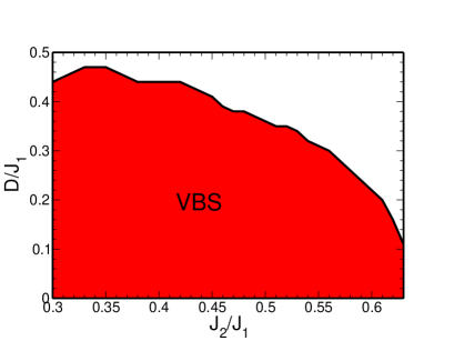
Figure 3: Region of stability of the columnar VBS phase [Fig. 1(c)] of the Heisenberg model (1) determined within the bond-operator formalism at the harmonic approximation. The external magnetic field $h_{z}=0.05\,J_{1}$.

The ground-state energy (38) in terms of the DM interaction $D$ and for fixed values of the exchange coupling $J_{2}$ is shown in Fig. 2(c). For all values of the coupling $J_{2}$, we find that the ground-state energy $E_{GS}$ decreases with the DM interaction $D$. Moreover, for a fixed DM interaction, we notice that $E_{GS}$ increases with the increasing of the exchange coupling $J_{2}$ up to $J_{2}\sim 0.57\,J_{1}$ and then it decreases. Indeed, for $D=h=0$, a quite similar behaviour was observed for the ground-state energy, namely, a monotonical increasing of $E_{GS}$ with $J_{2}$ up to $J_{2}=0.57\,J_{1}$ (see Fig. 3(a) from Ref. [93]).

         

         

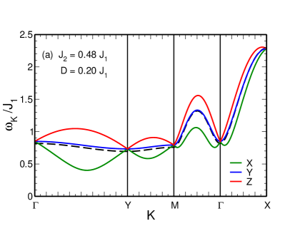
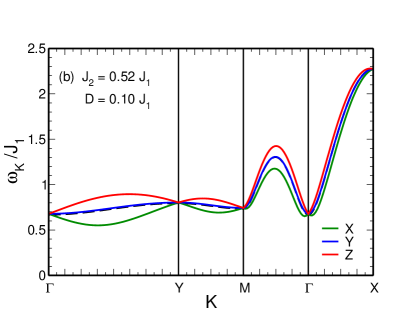
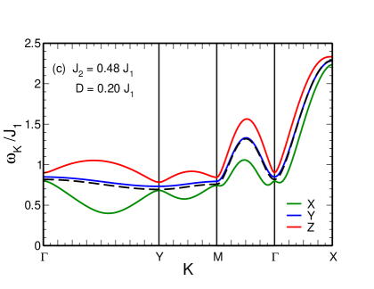
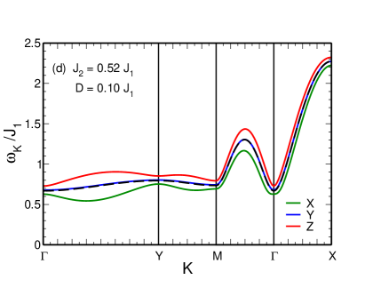
Figure 4: Triplon dispersion relations $\omega^{x}_{\bf k}$ (solid green line), $\omega^{y}_{\bf k}$ (solid blue line), and $\omega^{z}_{\bf k}$ (solid red line) [see Eq. (66)] of the columnar VBS phase at the harmonic approximation along paths in the dimerized Brillouin zone [Fig. 1(d)]: (a) and (c) $J_{2}=0.48\,J_{1}$ and $D=0.20\,J_{1}$ and (b) and (d) $J_{2}=0.52\,J_{1}$ and $D=0.10\,J_{1}$. The external magnetic field $h_{z}=0$ (upper panels) and $h_{z}=0.05\,J_{1}$ (lower panels). Dashed black line: triplon dispersion relation for the model (1) in the absence of the DM and Zeeman terms (see Fig. 4 from Ref. [93]).

Figures 4(a) and (c) show the energy $\omega^{\alpha}_{\bf k}$ of the triplon excitations for $J_{2}=0.48\,J_{1}$ and $D=0.20\,J_{1}$, with $h_{z}=0$ [Fig. 4(a)] and $h_{z}=0.05\,J_{1}$ [Fig. 4(c)] (solid lines), in addition to the triplon spectrum for $D=h=0$ (dashed black line), which is included here for comparison (see Fig. 4(a) from Ref. [93]). As expected for a VBS phase, the triplon excitation spectrum is gapped. One sees that the triple degeneracy of the triplon bands, a feature displayed by the $J_{1}$-$J_{2}$ model (2), is partially lifted by the DM interaction, since the triplon bands touch at the $\Gamma$, $\mathbf{X}$, $\mathbf{M}$, and $\mathbf{Y}$ points of the dimerized first Brillouin zone [see Fig. 1(d)] for $D\not=0$ and $h=0$ [Fig. 4(a)]. The three triplon bands are completely separated only in the presence of both DM interaction and external magnetic field [Fig. 4(c)]: Indeed, the DM interaction alone may not completely lift the degeneracy of an excitation spectrum as found, e.g., for magnons in magnets with long-range order [6, 7, 26]. Moreover, the triplon gap $\Delta$ (the minimum of the $\omega^{x}_{\bf k}$ triplon band) is associated with an incommensurate momentum ${\bf Q}=(0,1.7952)$, for $h_{z}=0.05\,J_{1}$; such a behaviour should be contrasted with the triplon spectrum for $D=h=0$, whose triplon gap is located at the (commensurate) $\mathbf{Y}$ point of the dimerized Brillouin zone. Similar considerations hold for the triplon excitation spectrum for $J_{2}=0.52\,J_{1}$ and $D=0.10\,J_{1}$, with $h_{z}=0$ [Fig. 4(b)] and $h_{z}=0.05\,J_{1}$ [Fig. 4(d)]: Here, the triplon gap is also located at an incommensurate momentum [${\bf Q}=(0,1.1669)$ for $h_{z}=0.05\,J_{1}$] while, for $D=h=0$, the triplon gap is at the centre of the dimerized Brillouin zone, the $\Gamma$ point. In the following, one considers a finite external magnetic field ($h_{z}=0.05\,J_{1}$), since one needs well separated triplon bands in order to properly define a Chern number and determine the topological aspect of the triplon excitations.

The behaviour of the triplon gap $\Delta$ in terms of the DM interaction $D$ for selected values of the exchange coupling $J_{2}$ is shown in Fig. 2(d). One sees that the triplon gap decreases with the DM interaction, regardless the value of the exchange coupling $J_{2}$. The smallest value of the gap, $\Delta\sim 0.12\,J_{1}$, corresponds to the parameter $D_{\rm max}$ above which numerical solutions for the self-consistent equations (LABEL:eqs-self) are no longer found. Moreover, as illustrated in Fig. 2(e), the momentum ${\bf Q}$ associated with the triplon gap moves along the $\Gamma$-$\mathbf{Y}$ line of the dimerized Brillouin zone: For $J_{2}<0.50\,J_{1}$, the momentum ${\bf Q}$ moves from the commensurate $\mathbf{Y}$ point to an incommensurate value ${\bf Q}=(0,Q_{y})$ as the DM interaction increases; for $J_{2}>0.50\,J_{1}$, the momentum ${\bf Q}$ moves from the commensurate $\Gamma$ point to an incommensurate momentum ${\bf Q}=(0,Q_{y})$ with the increasing of the parameter $D$. Such set of results indicates that the black line in Fig. 3 may signal a quantum phase transition from a VBS phase to a noncollinear long-range ordered magnetic phase with incommensurate ordering wave vector ${\bf Q}$. Due to the behaviour of the triplon gap $\Delta$ at the border of the VBS region shown in Fig. 3, at the moment, it is not clear whether such a quantum phase transition is a first-order transition or a continuous one; such an issue, which needs some further studies, is beyond the scope of our paper.

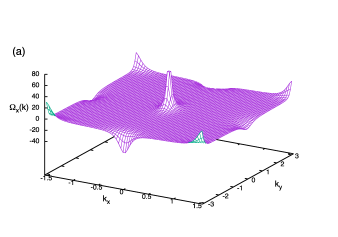
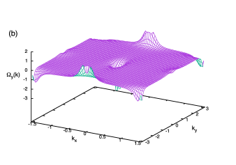
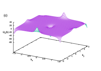
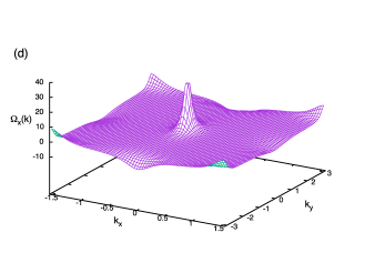
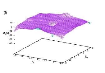
Figure 5: Berry curvatures $\Omega_{\alpha}({\bf k})$ [Eq. (45)] of the triplon dispersion relations $\omega^{\alpha}_{\bf k}$ shown in Fig. 4: (a) $\Omega_{x}({\bf k})$, (b) $\Omega_{y}({\bf k})$, and (c) $\Omega_{z}({\bf k})$ for $J_{2}=0.48\,J_{1}$ and $D=0.20\,J_{1}$; (d) $\Omega_{x}({\bf k})$, (e) $\Omega_{y}({\bf k})$, and (f) $\Omega_{z}({\bf k})$ for $J_{2}=0.52\,J_{1}$ and $D=0.10\,J_{1}$. The external magnetic field $h_{z}=0.05\,J_{1}$.

V Berry curvatures and Chern numbers

In this section, we study the topological properties of the triplon bands $\omega^{\alpha}_{\bf k}$. The main idea is to check whether the DM interaction (3), with the DM vectors (21), yields a columnar VBS phase for the square lattice $J_{1}$-$J_{2}$ model (2) with topologically nontrivial triplons, as previously found for a Heisenberg AFM on a Shastry-Sutherland lattice [14, 15, 16].

For quadratic bosonic Hamiltonians such as Eq. (31), which includes the anomalous terms $t_{-{\bf k},\alpha}t_{{\bf k},\beta}$ and $t^{\dagger}_{-{\bf k},\alpha}t^{\dagger}_{{\bf k},\beta}$, the Berry curvature $\Omega_{\alpha}({\bf k})$ of the (triplon) excitation band $\omega^{\alpha}_{\bf k}$ is given by [105, 106]

$$\Omega_{\alpha}({\bf k})=i\epsilon_{\mu\nu}\left[\hat{I}_{B}\frac{\partial\hat{T}_{\bf k}^{\dagger}}{\partial k_{\mu}}\hat{I}_{B}\frac{\partial\hat{T}_{\bf k}}{\partial k_{\nu}}\right]_{\alpha\alpha},$$ (45)

with $\alpha=1,2,\ldots,6$ and $\mu,\nu=x,y$. Here $\hat{I}_{B}$ and $\hat{T}_{\bf k}$ are, respectively, the $6\times 6$ matrices (36) and (42), $\epsilon_{\mu\nu}$ is the completely antisymmetric tensor with $\epsilon_{xy}=1$, and $[\quad]_{\alpha\alpha}$ indicates the diagonal element of the corresponding square matrix. Due to the form of the diagonal Hamiltonian (40), the Berry curvatures of the $\omega^{x}_{\bf k}$, $\omega^{y}_{\bf k}$, and $\omega^{z}_{\bf k}$ triplon bands are given by $\Omega_{1}({\bf k})\equiv\Omega_{x}({\bf k})$, $\Omega_{2}({\bf k})\equiv\Omega_{y}({\bf k})$, and $\Omega_{3}({\bf k})\equiv\Omega_{z}({\bf k})$, respectively. We calculate the Berry curvatures (45) of the triplon bands $\omega^{\alpha}_{\bf k}$ using the analytical expressions for the matrix elements of the $\hat{T}_{\bf k}$ matrix shown in Appendix C.

Figures 5(a), (b), and (c) show the Berry curvatures (45) respectively for the triplon bands $\omega^{x}_{\bf k}$, $\omega^{y}_{\bf k}$, and $\omega^{z}_{\bf k}$ displayed in Fig. 4(c), which correspond to the parameters $J_{2}=0.48\,J_{1}$, $D=0.20\,J_{1}$, and $h_{z}=0.05\,J_{1}$ of the model (1). For the three triplon bands, one sees that the Berry curvatures vanish for almost all points of the dimerized Brillouin zone [Fig. 1(d)], except in the vicinity of the $\Gamma$, $\mathbf{X}$, $\mathbf{M}$, and $\mathbf{Y}$ points. One notices that $\Omega_{x}({\bf k})\simeq-\Omega_{z}({\bf k})$, in addition to the fact that the peak intensities for $\Omega_{x}({\bf k})$ and $\Omega_{z}({\bf k})$ are larger than the corresponding ones for $\Omega_{y}({\bf k})$. Importantly, one verifies that the peak intensities of the Berry curvatures decrease as the DM interaction $D$ decreases and almost vanish for $D=10^{-3}\,J_{1}$ (the analytical expressions derived for the matrix elements of the $\hat{T}_{\bf k}$ matrix are not suitable for the case $D=0$, see Appendix C for details); such a feature indicates that the DM interaction (3), with the DM vectors (21), indeed yields a finite Berry curvature for the triplons. Similar qualitatively features are found for the three triplon bands shown in Fig. 4(d), which are associated with the parameters $J_{2}=0.52\,J_{1}$, $D=0.10\,J_{1}$, and $h_{z}=0.05\,J_{1}$, see Figs. 5(d), (e), and (f).

Table 1: Chern numbers of the $\omega^{x}_{\bf k}$, $\omega^{y}_{\bf k}$, and $\omega^{z}_{\bf k}$ triplon bands of the columnar VBS phase of the model (1) for $J_{2}=0.48$ and $J_{2}=0.52\,J_{1}$ and the DM interaction $D=0.10$ and $0.20\,J_{1}$. The external magnetic field $h_{z}=0.05\,J_{1}$.

				$J_{2}=0.48\,J_{1}$		$J_{2}=0.52\,J_{1}$
$D$		$\alpha$		$C_{\alpha}$		$C_{\alpha}$
$0.10$		$x$		$0$		$0$
$0.10$		$y$		$0$		$0$
$0.10$		$z$		$0$		$0$
$0.20$		$x$		$+2.08\times 10^{-4}$		$+1.07\times 10^{-3}$
$0.20$		$y$		$+2.09\times 10^{-4}$		$+0.88\times 10^{-3}$
$0.20$		$z$		$-4.18\times 10^{-4}$		$-1.95\times 10^{-3}$

Once the Berry curvatures $\Omega_{\alpha}({\bf k})$ of the triplon bands $\omega^{\alpha}_{\bf k}$ are determined, we can calculate the Chern number of each triplon band, which is defined as the integral of the Berry curvature over the dimerized Brillouin zone [105, 106], namely,

$$C_{\alpha}=\frac{1}{2\pi}\int_{BZ}d^{2}k\,\Omega_{\alpha}({\bf k}).$$ (46)

We determine the Chern numbers $C_{\alpha}$ via a numerical integration of Eq. (46).

The Chern numbers of the triplon bands for exchange couplings $J_{2}=0.48$ and $0.52\,J_{1}$ and DM interactions $D=0.10$ and $0.20\,J_{1}$ are displayed in Table 1. One finds that, regardless the value of the exchange coupling $J_{2}$ and the DM interaction $D$, the Chern numbers of the three triplon bands vanish: such results are related to the symmetries of the Berry curvatures, as exemplified in Fig. 5. Therefore, although the Berry curvatures are finite in some regions of the dimerized Brillouin zone, the triplon excitations of the columnar VBS phase of the Heisenberg model (1) are topologically trivial.

             

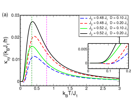
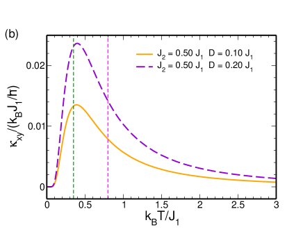
Figure 6: Thermal Hall conductivity $\kappa_{xy}/(k_{B}J_{1}/\hbar)$ as a function of the temperature $k_{B}T/J_{1}$ for the columnar VBS phase of the Heisenberg model (1). Next-nearest-neighbor exchange and DM couplings: (a) $J_{2}=0.48\,J_{1}$ and $D=0.10\,J_{1}$ (dashed blue line), $J_{2}=0.48\,J_{1}$ and $D=0.20\,J_{1}$ (dashed red line), $J_{2}=0.52\,J_{1}$ and $D=0.10\,J_{1}$ (solid green line), and $J_{2}=0.52\,J_{1}$ and $D=0.20\,J_{1}$ (solid black line); (b) $J_{2}=0.50\,J_{1}$ and $D=0.10\,J_{1}$ (solid orange line) and $J_{2}=0.50\,J_{1}$ and $D=0.20\,J_{1}$ (dashed violet line). The external magnetic field $h_{z}=0.05\,J_{1}$. The vertical dark-green dashed line indicates the temperature above which triplon-triplon interactions might be relevant; the vertical magenta dashed line is an estimate for the critical temperature $T_{c}$ above which the VBS phase is no longer stable (see text for details). Inset panel (a): low-temperature behaviour of the thermal Hall conductivity.

VI Thermal Hall conductivity

We now focus on the transport properties of the columnar VBS phase of the Heisenberg model (1), in particular, we determine the thermal Hall conductivity $\kappa_{xy}$ due to triplons. We follow the procedure proposed in Refs. [22, 23], where the thermal Hall conductivity $\kappa_{xy}$ due to the magnon excitations of a long-range ordered ferromagnet was determined; such a formalism was also applied to study the triplon thermal Hall effect in a AFM on a Shastry-Sutherland lattice [14, 15].

For a system of noniteracting boson excitations, the thermal Hall conductivity is given by [22, 23]

$$\kappa_{xy}=-\frac{k_{B}^{2}T}{\hbar V}\sum_{{\bf k},\alpha}c_{2}\left[f_{B}\left(\omega^{\alpha}_{\bf k}\right)\right]\Omega_{\alpha}({\bf k}),$$ (47)

where $k_{B}$ is the Boltzmann constant, $T$ is the temperature,

$$f_{B}(\epsilon)=\frac{1}{e^{\epsilon/k_{B}T}-1}$$ (48)

is the Bose distribution function, and $\Omega_{\alpha}({\bf k})$ is the Berry curvature (45) of the (bosonic) triplon excitation band $\omega^{\alpha}_{\bf k}$, with $\alpha=x,y,z$. Moreover, the function $c_{2}(x)$ assumes the form

$$c_{2}(x)= \int_{0}^{x}dt\left(\ln\frac{1+t}{t}\right)^{2}$$

$$= \left(1+x\right)\left(\ln\frac{1+x}{x}\right)^{2}-\left(\ln x\right)^{2}-2{\rm Li}_{2}(-x),$$ (49)

with ${\rm Li}_{2}(x)$ being the polylogarithm, which is defined as ${\rm Li}_{n}(z)=\sum_{j=1}^{\infty}z^{j}/j^{n}$; one shows that $c_{2}(x)$ is a monotonic function with $c_{2}(0)=0$ and $c_{2}(x\rightarrow\infty)=\pi^{2}/3$. We consider the Berry curvatures calculated in Sec. V and determine $\kappa_{xy}$ via a numerical integration of Eq. (47).

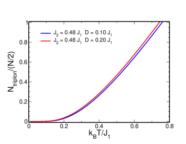
Figure 7: Number of triplons (50) as a function of the temperature $k_{B}T/J_{1}$ for the columnar VBS phase of the Heisenberg model (1) with $J_{2}=0.48\,J_{1}$ and DM couplings $D=0.10$ and $0.20\,J_{1}$. The external magnetic field $h_{z}=0.05\,J_{1}$. $N/2$ is the number of sites of the dimerized lattice $\mathcal{D}$ as illustrated in Fig. 1(c).

The behaviour of the thermal Hall conductivity (47) as a function of the temperature $T$ for $J_{2}=0.48$, $0.50$, and $0.52\,J_{1}$, DM interaction $D=0.10$ and $0.20\,J_{1}$, and external magnetic field $h_{z}=0.05\,J_{1}$ is shown in Fig. 6. One sees that, regardless the values of the exchange coupling $J_{2}$ and DM interaction $D$, the thermal Hall conductivities display a peak at $T\sim 0.5\,J_{1}/k_{B}$, whose height increases with the DM interaction for a fixed value of the exchange coupling $J_{2}$. Moreover, one notices that $\kappa_{xy}$ vanishes in the low-temperature region, a feature related to the existence of a finite triplon excitation gap, see Fig. 2(d). Interestingly, only for $J_{2}=0.48\,J_{1}$, $\kappa_{xy}$ assumes negative values around $T\sim 0.1\,J_{1}/k_{B}$ [see the inset of Fig. 6(a)]; indeed, for $J_{2}<0.50\,J_{1}$, we find a sign reversal of the thermal Hall conductivity as $T$ varies in this low-temperature region. Apart from the sign reversal in the low-temperature region and the fact that the triplons are topologically trivial, the behaviour of $\kappa_{xy}$ with the temperature $T$ qualitatively agrees with the phenomenological one discussed in Ref. [107].

A few remarks here about the temperature range below which our results for the thermal Hall conductivity might be valid are in order: The number of triplons as a function of the temperature is given by

$$N_{\rm triplons}=\sum_{{\bf k},\alpha}\langle b^{\dagger}_{{\bf k},\alpha}b_{{\bf k},\alpha}\rangle=\sum_{{\bf k},\alpha}f_{B}\left(\omega^{\alpha}_{\bf k}\right),$$ (50)

with $f_{B}(\epsilon)$ being the Bose distribution function (48). Figure 7 shows the behaviour of $N_{\rm triplons}$ with the temperature $T$ for $J_{2}=0.48\,J_{1}$, DM interaction $D=0.10$ and $0.20\,J_{1}$, and external magnetic field $h_{z}=0.05\,J_{1}$; we find a quite similar quantitative behaviour for $J_{2}=0.50$ and $0.52\,J_{1}$. One expects that, for $T\gtrsim 0.35\,k_{B}/J_{1}$ (dark-green dashed line in Fig. 6), the cubic terms (17) and (24) as well as the quartic terms (18) and (25), which are neglected in our study, might be relevant, and therefore, they could provide important corrections to the thermal Hall conductivity. Furthermore, for $T\gtrsim 0.8\,k_{B}/J_{1}$, one sees that the number of triplons $N_{\rm triplons}$ is larger than the number of sites $N^{\prime}=N/2$ of the dimerized lattice $\mathcal{D}$; such a feature indicates that, for $T\sim 0.8\,k_{B}/J_{1}$ (magenta dashed line in Fig. 6), the system might be close to the critical temperature $T_{c}$ above which the columnar VBS phase is no longer stable. We intend to investigate the effects of the triplon-triplon interaction on the thermal Hall conductivity in a future publication; such a study will also be important for a proper determination of the critical temperature $T_{c}$.

VII Summary and discussion

In spite of the fact that the triplon excitations are topologically trivial, the columnar VBS phase of the square-lattice AFM Heisenberg model (1) is characterized by a finite thermal Hall conductivity. Such a feature is indeed a thermal effect: Due to the weight function $c_{2}(x)$ [Eq. (49)], the integrand of Eq. (47) vanishes in the vicinity of the $\mathbf{X}$ point of the dimerized Brillouin zone (not shown here), implying a finite thermal Hall conductivity; recall that the Berry curvatures of the triplon bands are finite around the $\mathbf{X}$ point of the dimerized Brillouin zone (see Fig. 5), an important contribution that yields topologically trivial triplon excitations; as pointed out in Ref. [29], a VBS phase with topologically nontrivial triplons might be characterized by a thermal Hall conductivity qualitatively similar to the one found for the columnar VBS phase of the model (1), but with a higher peak at low temperatures.

The fact that a finite thermal Hall conductivity is found for the columnar VBS phase of the square-lattice AFM Heisenberg model (1) indicates that the no-go condition [21], which was determined for a long-range ordered magnet and is based on linear spin-wave theory results, does not apply for the columnar VBS phase. In fact, exceptions to the no-go condition [21] were previously reported. Kawano and Hotta [26] find a finite thermal Hall conductivity for a canted AFM ordered phase realized in a noncentrosymmetric square-lattice AFM; interestingly, the presence/absence of magnon edge modes is here characterized by a Z₂ topological invariant instead of a Chern number. Samajdar et al. [29] study a spin-liquid phase in a square-lattice AFM with a DM interaction term, whose DM vectors are associated with the spins in the CuO₂ planes of the La₂CuO₄ and YBCO compounds; the spin-liquid phase is described within the Schwinger-boson formalism; it was found that the thermal Hall conductivity is finite only when DM vectors related to the YBCO compound are considered; such a result is in agreement with a symmetry analysis also presented; moreover, although $\kappa_{xy}$ is finite, the (bosonic) spinon excitations of the spin-liquid phase are topologically trivial. Notice that the features found here for the columnar VBS phase are similar to the ones observed for the spin-liquid phase considered in Ref. [29].

A sign reversal of the thermal Hall conductivity with the increasing of the temperature $T$, from negative to positive values as we found for $J_{2}<0.50\,J_{1}$ in the low-temperature region, was also observed for ordered ferromagnets on the Shastry-Sutherland [7] and honeycomb [8] lattices. In particular, for a ferromagnet on the honeycomb lattice [8], it was pointed out that such a sign change indicates a topological phase transition, since a gap closure between the upper and lower magnon bands is also observed as $T$ varies, an effect due to magnon-magnon interactions. Such a similar gap closure is not observed in our case. At the moment, the sign reversal of $\kappa_{xy}$ for the columnar VBS phase of the model (1) with $J_{2}<0.50\,J_{1}$ is not completely understood; similarly to the phase diagram shown in Fig. 3, the low-temperature behaviour of $\kappa_{xy}$ seems to indicate a distinction between the parameter regions $J_{2}<0.5\,J_{1}$ and $J_{2}>0.5\,J_{1}$ of the $J_{1}$-$J_{2}$ model, which qualitatively agrees with Refs. [81, 83, 89, 94, 95, 97]; it is worth mentioning that one of us also find such a distinction in the study [93] concerning many-triplon states in the columnar VBS phase of the $J_{1}$-$J_{2}$ model.

In summary, in this paper we studied the spin-$1/2$ $J_{1}$-$J_{2}$ AFM Heisenberg model on a square lattice with an additional DM interaction between the spins and in the presence of an external magnetic field. We focused on the columnar VBS phase, which is stable within the intermediate parameter region of the $J_{1}$-$J_{2}$ model. In particular, we discussed the topological properties of the triplon excitations of the columnar VBS phase, which is described via an effective interacting boson model obtained with the aid of a bond-operator formalism for the spin operators. We considered the interacting boson model within a harmonic approximation and determined the triplon excitation bands. We found that the DM interaction provides a finite Berry curvature for the triplon bands, but the corresponding Chern numbers vanish. Although the triplon excitations are topologically trivial, we found that the thermal Hall conductivity of the columnar VBS phase is indeed finite.

Appendix A Effective boson model in real space

In this section, we provide the expressions of the Hamiltonians (12), (22), and (28) in terms of the singlet $s_{i}$ and triplet $t_{i\alpha}$ boson operators.

Let us first consider the $J_{1}$-$J_{2}$ AFM Heisenberg model (2). After substituting the generalized bond-operator expansion (9) of the spin operators in terms of the singlet and triplet operators, one arrives at the Hamiltonian (12), where the $\mathcal{H}_{J,n}$ terms read

$$\mathcal{H}_{J,0}= -\frac{3}{4}J_{1}\sum_{i}s_{i}^{\dagger}s_{i},$$

$$\mathcal{H}_{J,2}= \,\frac{J_{1}}{4}\sum_{i}t_{i\alpha}^{\dagger}t_{i\alpha}+\frac{1}{4}\sum_{i,\tau}\zeta_{2}(\tau)\left(s_{i}s_{i+\tau}^{\dagger}t_{i\alpha}^{\dagger}t_{i+\tau\alpha}+{\rm H.c.}\right.$$

$$\left.+\;s_{i}^{\dagger}s_{i+\tau}^{\dagger}t_{i\alpha}t_{i+\tau\alpha}+{\rm H.c.}\right),$$

$$\mathcal{H}_{J,3}= \,\frac{i}{4}\epsilon_{\alpha\beta\lambda}\sum_{i,\tau}\zeta_{3}(\tau)\Big{[}\left(s_{i}^{\dagger}t_{i\alpha}+t_{i\alpha}^{\dagger}s_{i}\right)t_{i+\tau\beta}^{\dagger}t_{i+\tau\lambda}\Big{.}$$

$$\Big{.}-\;(i\leftrightarrow i+\tau)\Big{]},$$

$$\mathcal{H}_{J,4}= -\frac{1}{4}\epsilon_{\alpha\beta\lambda}\>\epsilon_{\alpha\mu\nu}\sum_{i,\tau}\zeta_{4}(\tau)t_{i\beta}^{\dagger}t_{i+\tau\mu}^{\dagger}t_{i\lambda}t_{i+\tau\nu}.$$

Here the summation convention over repeated greek indices is implied, the $\zeta_{i}(\tau)$ functions are defined as

$$\zeta_{2}(\tau) = 2(J_{1}-J_{2})\delta_{\tau,2}-J_{1}\delta_{\tau,1}-J_{2}\left(\delta_{\tau,1+2}+\delta_{\tau,1-2}\right),$$

$$\zeta_{3}(\tau) = J_{1}\delta_{\tau,1}+J_{2}\left(\delta_{\tau,1+2}+\delta_{\tau,1-2}\right),$$

$$\zeta_{4}(\tau) = 2(J_{1}+J_{2})\delta_{\tau,2}+J_{1}\delta_{\tau,1}+J_{2}\left(\delta_{\tau,1+2}+\delta_{\tau,1-2}\right),$$

and the index $\tau$ indicates the dimer nearest-neighbor vectors $\mbox{\boldmath$\tau$}_{n}$ [see Eq. (11)]. It should be mentioned that, in order to derive the Hamiltonian (12), it is convenient to consider the identity

$${\bf S}^{1}\cdot{\bf S}^{2}=-\frac{3}{4}s^{\dagger}s+\frac{1}{4}\sum_{\alpha}t^{\dagger}_{\alpha}t_{\alpha}$$ (52)

for the local term $J_{1}({\bf S}^{1}_{i}\cdot{\bf S}^{2}_{i})$ of the Hamiltonian (10) and the expansion (9) for the nonlocal ones.

Concerning the DM interaction (3), the local term of the Hamiltonian (20), ${\bf D}_{i,i}\cdot({\bf S}_{i}^{1}\times{\bf S}_{i}^{2})$, can be easily treated with the aid of the identity

$${\bf D}\cdot\left({\bf S}^{1}\times{\bf S}^{2}\right)=\frac{1}{2}iD_{\alpha}s^{\dagger}t_{\alpha}+{\rm H.c.},$$ (53)

which can be obtained following the same procedure that yields the identity (52). Similarly to the $J_{1}$-$J_{2}$ model (2), one employs the expansion (9) for the nonlocal terms of the Hamiltonian (20), and shows that the four terms of the effective boson model (22) assume the form

$$\mathcal{H}_{\rm DM,1}= \frac{1}{2}iDs_{i}^{\dagger}t_{ix}+{\rm H.c.},$$

$$\mathcal{H}_{\rm DM,2}= -\frac{1}{4}D\,\epsilon_{x\beta\gamma}\sum_{i\in\mathcal{D}}\left(s^{\dagger}_{i+1}s_{i}t_{i\beta}^{\dagger}t_{i+1,\gamma}+{\rm H.c.}\right.$$

$$+\left.s_{i}^{\dagger}s_{i+1}^{\dagger}t_{i\beta}t_{i+1,\gamma}+{\rm H.c.}\right)$$

$$-\frac{1}{2}D\,\epsilon_{y\beta\gamma}\sum_{i\in\mathcal{D}}\left(s^{\dagger}_{i+2}s_{i}t_{i\beta}^{\dagger}t_{i+2,\gamma}+{\rm H.c.}\right.$$

$$+\left.s_{i}^{\dagger}s_{i+2}^{\dagger}t_{i\beta}t_{i+2,\gamma}+{\rm H.c.}\right),$$

$$\mathcal{H}_{\rm DM,3}= \frac{1}{4}iD\,\epsilon_{x\beta\gamma}\sum_{i\in\mathcal{D}}\epsilon_{\gamma\mu\nu}\left(s_{i}^{\dagger}t_{i\beta}+t^{\dagger}_{i\beta}s_{i}\right)t_{i+1,\mu}^{\dagger}t_{i+1,\nu}$$

$$-\epsilon_{\beta\mu\nu}\,t_{i\mu}^{\dagger}t_{i\nu}\left(s_{i+1}^{\dagger}t_{i+1,\gamma}+t^{\dagger}_{i+1,\gamma}s_{i+1}\right),$$

$$\mathcal{H}_{\rm DM,4}= -D\,\epsilon_{\beta\mu\nu}\epsilon_{\gamma\mu^{\prime}\nu^{\prime}}\sum_{i\in\mathcal{D}}\left(\frac{1}{4}\,\epsilon_{x\beta\gamma}\,t_{i\mu}^{\dagger}t_{i\nu}t_{i+1,\mu^{\prime}}^{\dagger}t_{i+1,\nu^{\prime}}\right.$$

$$-\left.\frac{1}{2}\,\epsilon_{y\beta\gamma}\,t_{i\mu}^{\dagger}t_{i\nu}t_{i+2,\mu^{\prime}}^{\dagger}t_{i+2,\nu^{\prime}}\right).$$

Finally, one easily shows that, in terms of the singlet and triplet operators, the Zeeman term (28) is given by

$$\mathcal{H}_{B}=i\epsilon_{\alpha\beta\gamma}\sum_{i\in\mathcal{D}}h_{\alpha}\,t_{i\beta}^{\dagger}t_{i\gamma},$$ (55)

where $h_{\alpha}$, with $\alpha=x,y,z$, is the $\alpha$-component of the external magnetic field ${\bf h}=g\mu_{B}{\bf B}$.

Appendix B Linear triplet term of the effective boson model

In this section, we provide some details of the procedure employed to treat the linear triplet term $\mathcal{H}_{\rm DM,1}$ of the effective boson model [see Eq. (LABEL:h-boson2ap)]. In particular, we adopted the treatment described in Ref. [16].

As mentioned in Sec. III.1, the linear term $\mathcal{H}_{\rm DM,1}$ can be removed via an unitary transformation performed in each site of the dimerized lattice $\mathcal{D}$. Since $\mathcal{H}_{\rm DM,1}$ couples the singlet $s_{i}$ and the triplet $t_{ix}$ operators, we consider the Hamiltonian

$$H_{L}= \,\mathcal{H}_{J,0}+\mathcal{H^{\prime}}_{J,2}+\mathcal{H}_{\rm DM,1}$$

$$= \,J_{1}\sum_{i}\left(-\frac{3}{4}s_{i}^{\dagger}s_{i}+\frac{1}{4}t_{ix}^{\dagger}t_{ix}+i\frac{D}{2J_{1}}s_{i}^{\dagger}t_{ix}+{\rm H.c.}\right),$$ (56)

which includes the local terms $\mathcal{H}_{J,0}$ and $\mathcal{H^{\prime}}_{J,2}$ related to the $J_{1}$-$J_{2}$ model [see Eq. (LABEL:h-boson1ap)] and the local one $\mathcal{H}_{\rm DM,1}$ derived from the DM interaction [see Eq. (LABEL:h-boson2ap)].

In matrix form, the Hamiltonian (56) reads

$$H_{L}=J_{1}\sum_{i\in\mathcal{D}}\begin{pmatrix}s_{i}^{\dagger}&t_{ix}^{\dagger}\end{pmatrix}\begin{pmatrix}-\frac{3}{4}&i\alpha\\ -i\alpha&\frac{1}{4}\end{pmatrix}\begin{pmatrix}s_{i}\\ t_{ix}\end{pmatrix},$$ (57)

with the parameter $\alpha=D/(2J_{1})$ defined in terms of the DM interaction $D$ and the nearest-neighbor exchange coupling $J_{1}$. It is quite easy to show that the Hamiltonian (57) can be diagonalized by an unitary transformation defined by the unitary matrix

$$U=\frac{1}{\sqrt{2\left(b^{2}-b\right)}}\begin{pmatrix}2\alpha&i(1-b)\\ i(1-b)&2\alpha\end{pmatrix},$$ (58)

with $b=(1+4\alpha^{2})^{1/2}$. Assuming that $\alpha\ll 1$, one finds that $b^{2}-b\approx 2\alpha^{2}$ and $1-b\approx-2\alpha^{2}$, and therefore, up to linear order in the parameter $\alpha$, the unitary matrix (58) reads

$$U\approx\begin{pmatrix}1&-i\alpha\\ -i\alpha&1\end{pmatrix}.$$ (59)

With the aid of the Eq. (59), one defines a new set of singlet $\tilde{s}_{i}$ and triplet $\tilde{t}_{i\alpha}$ boson operators,

$$\begin{pmatrix}\tilde{s}_{i}\\ \tilde{t}_{ix}\\ \tilde{t}_{iy}\\ \tilde{t}_{iz}\end{pmatrix}=\begin{pmatrix}1&-i\alpha&0&0\\ -i\alpha&1&0&0\\ 0&0&1&0\\ 0&0&0&1\end{pmatrix}\begin{pmatrix}s_{i}\\ t_{ix}\\ t_{iy}\\ t_{iz}\end{pmatrix},$$ (60)

and shows that the Hamiltonian (56) assumes a diagonal form, namely,

$$H_{L}=J_{1}\sum_{i\in\mathcal{D}}\left(-\frac{3}{4}\tilde{s}_{i}^{\dagger}\tilde{s}_{i}+\frac{1}{4}\tilde{t}_{ix}^{\dagger}\tilde{t}_{ix}\right).$$ (61)

Substituting the inverse of the transformation (60) in Eqs. (LABEL:h-boson1ap), (LABEL:h-boson2ap), and (55), one finds the expression of the effective boson model in terms of the singlet $\tilde{s}_{i}$ and triplet $\tilde{t}_{i\alpha}$ boson operators. In particular, it is easy to show that, up to linear order in the parameter $\alpha$, the quadratic terms $\mathcal{H}_{J,2}$ and $\mathcal{H}_{\rm DM,2}$ assume the forms shown in Eqs. (LABEL:h-boson2ap) and (55), respectively, with the replacements $s_{i}\rightarrow\tilde{s}_{i}$ and $t_{i\alpha}\rightarrow\tilde{t}_{i\alpha}$. Moreover, one also finds that, up to linear order in the parameter $\alpha$, the cubic term $\mathcal{H}_{J,3}$ yields an additional quadratic term, namely,

$$\mathcal{H}=-i\epsilon_{x\beta\gamma}\sum_{\bf k}D^{\prime}_{\bf k}\left[\tilde{t}^{\dagger}_{{\bf k}\beta}\tilde{t}_{{\bf k}\gamma}+\frac{1}{2}\left(\tilde{t}_{-{\bf k}\beta}\tilde{t}_{{\bf k}\gamma}-\tilde{t}^{\dagger}_{-{\bf k}\beta}\tilde{t}^{\dagger}_{{\bf k}\gamma}\right)\right],$$ (62)

with

$$D^{\prime}_{\bf k}= \frac{1}{2}DN_{0}\sin(2k_{x})+\frac{1}{2}DN_{0}\frac{J_{2}}{J_{1}}\left[\sin\left(2k_{x}+k_{y}\right)\right.$$

$$\left.+\sin\left(2k_{x}-k_{y}\right)\right].$$ (63)

Therefore, the quadratic Hamiltonian (30), considered within the harmonic approximation, assumes the form defined by Eqs. (31)-(35), with the replacements $t_{i\alpha}\rightarrow\tilde{t}_{i\alpha}$ and $D_{\bf k}\rightarrow D_{\bf k}+D^{\prime}_{\bf k}$, see Eq. (27). In Sec. IV, after performing such replacements, we restore the notation for the triplet operators, i.e., $\tilde{t}_{i\alpha}\rightarrow t_{i\alpha}$.

A few remarks here about the Zeeman term (55) are in order: In principle, the Zeeman term should also be included in the Hamiltonian (56); since we consider a very small external magnetic field, $h_{z}=0.05\,J_{1}$, we neglect the contribution of the Zeeman term to the (local) Hamiltonian (56); importantly, the results derived in Sec. IV within the harmonic approximation for $D<h_{z}$ may need some further corrections.

Appendix C Details about the diagonalization of the harmonic Hamiltonian

In this appendix, we present the analytical expressions of the triplon dispersion relations $\omega^{\alpha}_{\bf k}$, in addition to the matrix elements of the $\hat{T}_{\bf k}$ matrix (42), which relates the triplet $t$ and triplon $b$ boson operators, see Eq. (41). The analytical procedure employed here is based on Refs. [103, 104] and it was previously applied by one of us to diagonalize a $4\times 4$ and a $6\times 6$ boson Hamiltonians, see Refs. [108] and [80], respectively.

As mentioned in Sec. IV, instead of the $\hat{H}_{\bf k}$ matrix (34), one should diagonalize the $\hat{I}_{B}\hat{H}_{\bf k}$ matrix (36). One finds that the eigenvalues $\omega^{\alpha}_{\bf k}$ are the roots of the polynomial

$$(\omega^{\alpha}_{\bf k})^{6}+a_{2,{\bf k}}(\omega^{\alpha}_{\bf k})^{4}+a_{1,{\bf k}}(\omega^{\alpha}_{\bf k})^{2}+a_{0,{\bf k}}=0,$$ (64)

where the coefficients $a_{i,{\bf k}}$ are written in terms of the coefficients $A_{\bf k}$ and $B_{\bf k}$ defined by Eq. (LABEL:coefs01), the coefficients $C_{\bf k}$ and $D_{\bf k}$ respectively given by Eqs. (26) and (27), and the external magnetic field $h_{z}$:

$$a_{0,{\bf k}}= \left(B_{\bf k}-A_{\bf k}\right)\left(B_{\bf k}^{2}+h_{z}^{2}-A_{\bf k}^{2}\right)\left[B_{\bf k}\left(B_{\bf k}^{2}+h_{z}^{2}-4D_{\bf k}^{2}-4C_{\bf k}^{2}\right)+A_{\bf k}\left(B_{\bf k}^{2}+h_{z}^{2}+4D_{\bf k}^{2}+4C_{\bf k}^{2}\right)-A_{\bf k}^{2}\left(A_{\bf k}+B_{\bf k}\right)\right],$$

$$a_{1,{\bf k}}= \,h_{z}^{4}+\left(A_{\bf k}-B_{\bf k}\right)^{2}\left[3\left(A_{\bf k}+B_{\bf k}\right)^{2}-4\left(C_{\bf k}^{2}+D_{\bf k}^{2}\right)\right],$$ (65)

$$a_{2,{\bf k}}= -3\left(A_{\bf k}^{2}-B_{\bf k}^{2}\right)-2h_{z}^{2}.$$

Due to the form of Eq. (64), one sees that the eigenvalues $(\omega^{\alpha}_{\bf k})^{2}$ are indeed the roots of a cubic polynomial which can be written as

$$\omega_{\bf k}^{x/y} =\left[-\frac{1}{3}a_{2,{\bf k}}-\frac{1}{2}\left(P_{1,{\bf k}}+P_{2,{\bf k}}\right)\pm i\frac{\sqrt{3}}{2}\left(P_{1,{\bf k}}-P_{2,{\bf k}}\right)\right]^{1/2},$$

$$\omega_{\bf k}^{z} =\left[-\frac{1}{3}a_{2,{\bf k}}+\left(P_{1,{\bf k}}+P_{2,{\bf k}}\right)\right]^{1/2},$$ (66)

where,

$$P_{1/2,{\bf k}}= \left(M_{\bf k}\pm\sqrt{N_{\bf k}}\right)^{1/3},\quad\quad\quad N_{\bf k}=Q_{\bf k}^{3}+M_{\bf k}^{2},\quad\quad\quad Q_{\bf k}=\frac{1}{9}\left(3a_{1,{\bf k}}-a_{2,{\bf k}}^{2}\right),$$

$$M_{\bf k}= \frac{1}{54}\left(9a_{2,{\bf k}}a_{1,{\bf k}}-27a_{0,{\bf k}}-2a_{2,{\bf k}}^{3}\right).$$ (67)

In order to determine the matrix elements of the $\hat{T}_{\bf k}$ matrix (42), it is interesting to consider the two eigenvalue problems

$$\hat{I}_{B}\hat{H^{\prime}}_{\bf k}\hat{Z}^{i}_{1,{\bf k}}-\omega_{\bf k}^{i}\hat{Z}^{i}_{1,{\bf k}}=0,\quad\quad\quad{\rm and}\quad\quad\quad\hat{I}_{B}\hat{H^{\prime}}_{\bf k}\hat{Z}^{i}_{2,{\bf k}}+\omega_{\bf k}^{i}\hat{Z}^{i}_{2,{\bf k}}=0,$$ (68)

with $\omega^{i}_{\bf k}>0$ and $i=1,2,3$. Here the six-component vectors $\hat{Z}^{i}_{1/2,{\bf k}}$ are defined as

$$\hat{Z}^{i}_{1,{\bf k}} =\begin{pmatrix}u^{i1}_{\bf k}&u^{i2}_{\bf k}&u^{i3}_{\bf k}&v^{i1}_{\bf k}&v^{i2}_{\bf k}&v^{i3}_{\bf k}\end{pmatrix}^{T},\quad\quad\quad{\rm and}\quad\quad\quad\hat{Z}^{i}_{2,{\bf k}}=\begin{pmatrix}y^{i1}_{\bf k}&y^{i2}_{\bf k}&y^{i3}_{\bf k}&x^{i1}_{\bf k}&x^{i2}_{\bf k}&x^{i3}_{\bf k}\end{pmatrix}^{T}$$

and one identifies $\omega_{\bf k}^{1}=\omega^{x}_{\bf k}$, $\omega_{\bf k}^{2}=\omega^{y}_{\bf k}$, and $\omega_{\bf k}^{3}=\omega^{z}_{\bf k}$. Equation (68) allows one to determine (i) the elements $u^{i1}_{\bf k}$, $u^{i2}_{\bf k}$, $u^{i3}_{\bf k}$, $v^{i1}_{\bf k}$, and $v^{i2}_{\bf k}$ in terms of the element $v^{i3}_{\bf k}$ and (ii) the elements $y^{i1}_{\bf k}$, $y^{i2}_{\bf k}$, $y^{i3}_{\bf k}$, $x^{i1}_{\bf k}$, and $x^{i2}_{\bf k}$ in terms of the element $x^{i3}_{\bf k}$, for $i=1,2,3$. Moreover, the condition (43) allows one to determine the elements $v^{i3}_{\bf k}$ and $x^{i3}_{\bf k}$. Indeed, it is useful to write the matrix elements of the $3\times 3$ matrices $\hat{U}_{\bf k}$, $\hat{V}_{\bf k}$, $\hat{X}_{\bf k}$, and $\hat{Y}_{\bf k}$ in terms of the (auxiliary) elements $\bar{u}_{ij,{\bf k}}$, $\bar{v}_{ij,{\bf k}}$, $\bar{x}_{ij,{\bf k}}$, and $\bar{y}_{ij,{\bf k}}$ as

$$\hat{U}_{\bf k}= \begin{pmatrix}v^{31}_{\bf k}\bar{u}_{11,{\bf k}}&v^{32}_{\bf k}\bar{u}_{42,{\bf k}}&v^{33}_{\bf k}\bar{u}_{73,{\bf k}}\\ v^{31}_{\bf k}\bar{u}_{21,{\bf k}}&v^{32}_{\bf k}\bar{u}_{52,{\bf k}}&v^{33}_{\bf k}\bar{u}_{83,{\bf k}}\\ v^{31}_{\bf k}\bar{u}_{31,{\bf k}}&v^{32}_{\bf k}\bar{u}_{62,{\bf k}}&v^{33}_{\bf k}\bar{u}_{93,{\bf k}}\end{pmatrix}, \hat{Y}_{\bf k}=\begin{pmatrix}x^{31}_{\bf k}\bar{y}_{11,{\bf k}}&x^{32}_{\bf k}\bar{y}_{42,{\bf k}}&x^{33}_{\bf k}\bar{y}_{73,{\bf k}}\\ x^{31}_{\bf k}\bar{y}_{21,{\bf k}}&x^{32}_{\bf k}\bar{y}_{52,{\bf k}}&x^{33}_{\bf k}\bar{y}_{83,{\bf k}}\\ x^{31}_{\bf k}\bar{y}_{31,{\bf k}}&x^{32}_{\bf k}\bar{y}_{62,{\bf k}}&x^{33}_{\bf k}\bar{y}_{93,{\bf k}}\end{pmatrix},$$

$$\hat{V}_{\bf k}= \begin{pmatrix}v^{31}_{\bf k}\bar{v}_{11,{\bf k}}&v^{32}_{\bf k}\bar{v}_{42,{\bf k}}&v^{33}_{\bf k}\bar{v}_{73,{\bf k}}\\ v^{31}_{\bf k}\bar{v}_{21,{\bf k}}&v^{32}_{\bf k}\bar{v}_{52,{\bf k}}&v^{33}_{\bf k}\bar{v}_{83,{\bf k}}\\ v^{31}_{\bf k}\ &v^{32}_{\bf k}&v^{33}_{\bf k}\end{pmatrix}, \hat{X}_{\bf k}=\begin{pmatrix}x^{31}_{\bf k}\bar{x}_{11,{\bf k}}&x^{32}_{\bf k}\bar{x}_{42,{\bf k}}&x^{33}_{\bf k}\bar{x}_{73,{\bf k}}\\ x^{31}_{\bf k}\bar{x}_{21,{\bf k}}&x^{32}_{\bf k}\bar{x}_{52,{\bf k}}&x^{33}_{\bf k}\bar{x}_{83,{\bf k}}\\ x^{31}_{\bf k}&x^{32}_{\bf k}&x^{33}_{\bf k}\end{pmatrix}.$$

With the aid of the condition (43), one then shows that

$$v^{3,j}_{\bf k}= \left(\left|\bar{u}_{3j-2,1,{\bf k}}\right|^{2}-\left|\bar{v}_{3j-2,1,{\bf k}}\right|^{2}+\left|\bar{u}_{3j-1,1,{\bf k}}\right|^{2}-\left|\bar{v}_{3j-1,1,{\bf k}}\right|^{2}-1+\left|\bar{u}_{3j,1,{\bf k}}\right|^{2}\right)^{-1/2},$$

$$x^{3,j}_{\bf k}= \left(\left|\bar{x}_{3j-2,1,{\bf k}}\right|^{2}-\left|\bar{y}_{3j-2,1,{\bf k}}\right|^{2}+\left|\bar{x}_{3j-1,1,{\bf k}}\right|^{2}-\left|\bar{y}_{3j-1,1,{\bf k}}\right|^{2}+1-\left|\bar{y}_{3j,1,{\bf k}}\right|^{2}\right)^{-1/2},$$

for $j=1,2,3$. The two eigenvalue problems (68) allow one to determine the elements $\bar{u}_{ij,{\bf k}}$, $\bar{v}_{ij,{\bf k}}$, $\bar{x}_{ij,{\bf k}}$, and $\bar{y}_{ij,{\bf k}}$. One then finds that the elements $\bar{u}_{ij,{\bf k}}$ assume the form

$$\bar{u}_{\alpha\beta,{\bf k}}= \,i\frac{1}{F_{\beta,{\bf k}}}\left(B_{\bf k}+R_{\beta,{\bf k}}\right)\Big{[}B_{\bf k}^{3}C_{\bf k}+B_{\bf k}^{2}\left(L_{4,{\bf k}}-C_{\bf k}S_{\beta,{\bf k}}\right)+\left(L_{4,{\bf k}}+C_{\bf k}R_{\beta,{\bf k}}\right)\left(h_{z}^{2}-S_{\beta,{\bf k}}^{2}\right)\Big{.}$$

$$\Big{.}+\,B_{\bf k}\left(h_{z}^{2}C_{\bf k}+2L_{4,{\bf k}}\omega_{\bf k}^{\beta}+C_{\bf k}R_{\beta,{\bf k}}S_{\beta,{\bf k}}\right)\Big{]},\quad\quad\quad{\rm for}\quad\quad\quad\alpha=1,4,7,$$

$$\bar{u}_{\alpha\beta,{\bf k}}= \frac{1}{F_{\beta,{\bf k}}}\Big{[}iL_{1,{\bf k}}L_{6,{\bf k}}\left(L_{5,{\bf k}}-D_{\bf k}L_{6,{\bf k}}\right)+h_{z}\left(2B_{\bf k}L_{4,{\bf k}}+3B_{\bf k}^{2}C_{\bf k}+h_{z}^{2}C_{\bf k}-2A_{\bf k}L_{4,{\bf k}}-4A_{\bf k}B_{\bf k}C_{\bf k}+A_{\bf k}^{2}C_{\bf k}\right)\omega_{\bf k}^{\beta}\Big{.}$$

$$\Big{.}-\,\left(ih_{z}^{2}D_{\bf k}-2iA_{\bf k}D_{\bf k}L_{6,{\bf k}}-h_{z}C_{\bf k}L_{6,{\bf k}}\right)(\omega_{\bf k}^{\beta})^{2}-h_{z}C_{\bf k}(\omega_{\bf k}^{\beta})^{3}+iD_{\bf k}(\omega_{\bf k}^{\beta})^{4}\Big{]},\quad\quad{\rm for}\quad\quad\alpha=2,5,8,$$

$$\bar{u}_{\alpha\beta,{\bf k}}= \frac{1}{F_{\beta,{\bf k}}}\Big{[}B_{\bf k}L_{1,{\bf k}}\left(2L_{2,{\bf k}}+A_{\bf k}^{2}-h_{z}^{2}\right)-L_{1,{\bf k}}\left(B_{\bf k}^{3}+2A_{\bf k}L_{2,{\bf k}}\right)-2\left(B_{\bf k}^{3}+A_{\bf k}L_{2,{\bf k}}\right)(\omega_{\bf k}^{\beta})^{2}\Big{.}$$

$$\Big{.}+\,B_{\bf k}\left(h_{z}^{2}+A_{\bf k}^{2}+L_{2,{\bf k}}\right)(\omega_{\bf k}^{\beta})^{2}-B_{\bf k}(\omega_{\bf k}^{\beta})^{4}\Big{]},\quad\quad\quad{\rm for}\quad\quad\quad\alpha=3,6,9,$$

the elements $\bar{v}_{ij,{\bf k}}$ are given by

$$\bar{v}_{\alpha\beta,{\bf k}}= +i\frac{1}{F_{\alpha,{\bf k}}}\left(B_{\bf k}+R_{\alpha,{\bf k}}\right)\Big{[}B_{\bf k}^{3}C_{\bf k}+B_{\bf k}^{2}\left(C_{\bf k}R_{\alpha,{\bf k}}-L_{4,{\bf k}}\right)-i\left(h_{z}+R_{\alpha,{\bf k}}\right)\left(h_{z}+R_{\alpha,{\bf k}}\right)\left(+h_{z}D_{\bf k}+iC_{\bf k}S_{\alpha,{\bf k}}\right)\Big{.}$$

$$+\,B_{\bf k}\left(h_{z}^{2}C_{\bf k}+2L_{4,{\bf k}}\omega_{\bf k}^{\alpha}+C_{\bf k}R_{\alpha,{\bf k}}S_{\alpha,{\bf k}}\right)\Big{]},\quad\quad\quad{\rm for}\quad\quad\quad\alpha=1,4,7,$$

$$\bar{v}_{\alpha\beta,{\bf k}}= -i\,\frac{1}{F_{\alpha,{\bf k}}}\left(B_{\bf k}+R_{\alpha,{\bf k}}\right)\Big{[}B_{\bf k}^{3}D_{\bf k}+B_{\bf k}^{2}\left(D_{\bf k}R_{\alpha,{\bf k}}+L_{5,{\bf k}}\right)-i\left(h_{z}+R_{\alpha,{\bf k}}\right)\left(R_{\alpha,{\bf k}}-h_{z}\right)\left(-h_{z}C_{\bf k}+iD_{\bf k}S_{\alpha,{\bf k}}\right)\Big{.}$$

$$+\,B_{\bf k}\left(h_{z}^{2}D_{\bf k}-2L_{5,{\bf k}}\omega_{\bf k}^{\alpha}+D_{\bf k}R_{\alpha,{\bf k}}S_{\alpha,{\bf k}}\right)\Big{]},\quad\quad\quad{\rm for}\quad\quad\quad\alpha=2,5,8,$$

the elements $\bar{y}_{\alpha\beta,{\bf k}}$ read

$$\bar{y}_{\alpha\beta,{\bf k}}= \frac{1}{G_{\beta,{\bf k}}}\Big{[}+iB_{\bf k}^{4}C_{\bf k}-B_{\bf k}^{3}\left(2iA_{\bf k}C_{\bf k}-h_{z}D_{\bf k}\right)-\left(h_{z}+R_{\beta,{\bf k}}\right)\left(R_{\beta,{\bf k}}-h_{z}\right)\left(-h_{z}D_{\bf k}+iC_{\bf k}S_{\beta,{\bf k}}\right)S_{\beta,{\bf k}}\Big{.}$$

$$\Big{.}+\,B_{\bf k}\left(h_{z}^{3}D_{\bf k}-2ih_{z}^{2}C_{\bf k}S_{\beta,{\bf k}}-2iA_{\bf k}C_{\bf k}R_{\beta,{\bf k}}S_{\beta,{\bf k}}\right)-h_{z}B_{\bf k}D_{\bf k}\left(A_{\bf k}^{2}-4A_{\bf k}\omega_{\bf k}^{\beta}-(\omega_{\bf k}^{\beta})^{2}\right)\Big{.}$$

$$\Big{.}-h_{z}B_{\bf k}^{2}D_{\bf k}\left(A_{\bf k}+3\omega_{\bf k}^{\beta}\right)-h_{z}B_{\bf k}^{2}L_{5,{\bf k}}\Big{]},\quad\quad\quad{\rm for}\quad\quad\quad\alpha=1,4,7,$$

$$\bar{y}_{\alpha\beta,{\bf k}}= \frac{1}{G_{\beta,{\bf k}}}\Big{[}-iB_{\bf k}^{4}D_{\bf k}+B_{\bf k}^{3}\left(2iA_{\bf k}D_{\bf k}+h_{z}C_{\bf k}\right)+\left(h_{z}+R_{\beta,{\bf k}}\right)\left(R_{\beta,{\bf k}}-h_{z}\right)\left(+h_{z}C_{\bf k}+iD_{\bf k}S_{\beta,{\bf k}}\right)S_{\beta,{\bf k}}\Big{.}$$

$$\Big{.}+\,B_{\bf k}\left(h_{z}^{3}C_{\bf k}+2ih_{z}^{2}D_{\bf k}S_{\beta,{\bf k}}+2iA_{\bf k}D_{\bf k}R_{\beta,{\bf k}}S_{\beta,{\bf k}}\right)-h_{z}B_{\bf k}C_{\bf k}\left(A_{\bf k}^{2}-4A_{\bf k}\omega_{\bf k}^{\beta}-(\omega_{\bf k}^{\beta})^{2}\right)\Big{.}$$

$$\Big{.}-\,h_{z}B_{\bf k}^{2}C_{\bf k}\left(A_{\bf k}+3\omega_{\bf k}^{\beta}\right)+h_{z}B^{2}_{\bf k}L_{4,{\bf k}}\Big{]},\quad\quad\quad{\rm for}\quad\quad\quad\alpha=2,5,8,$$

$$\bar{y}_{\alpha\beta,{\bf k}}= \frac{1}{G_{\beta,{\bf k}}}\Big{[}B_{\bf k}L_{1,{\bf k}}\left(2L_{2,{\bf k}}+A_{\bf k}^{2}-h_{z}^{2}\right)-L_{1,{\bf k}}\left(B_{\bf k}^{3}+2A_{\bf k}L_{2,{\bf k}}\right)\Big{.}-2\left(B_{\bf k}^{3}+A_{\bf k}L_{2,{\bf k}}\right)(\omega_{\bf k}^{\beta})^{2}$$

$$\Big{.}+B_{\bf k}\left(h_{z}^{2}+A_{\bf k}^{2}+L_{2}\right)(\omega_{\bf k}^{\beta})^{2}-B_{\bf k}(\omega_{\bf k}^{\beta})^{4}\Big{]},\quad\quad{\rm for}\quad\quad\quad\alpha=3,6,9,$$

and the elements $\bar{x}_{i,{\bf k}}$ are given by

$$\bar{x}_{\alpha\beta,{\bf k}}= +i\frac{1}{G_{\beta,{\bf k}}}\left(B_{\bf k}-S_{\beta,{\bf k}}\right)\Big{[}B_{\bf k}^{3}C_{\bf k}+\left(h_{z}-S_{\beta,{\bf k}}\right)\left(h_{z}+S_{\beta,{\bf k}}\right)\left(C_{\bf k}R_{\beta,{\bf k}}-L_{4,{\bf k}}\right)\Big{.}$$

$$\Big{.}-B_{\bf k}^{2}\left(L_{4,{\bf k}}+C_{\bf k}S_{\beta,{\bf k}}\right)+B_{\bf k}\left(h_{z}^{2}C_{\bf k}-2L_{4,{\bf k}}\omega_{\bf k}^{\beta}+C_{\bf k}R_{\beta,{\bf k}}S_{\beta,{\bf k}}\right)\Big{]}, {\rm for}\quad\quad\quad\alpha=1,4,7,$$

$$\bar{x}_{\alpha\beta,{\bf k}}= -i\frac{1}{G_{\beta,{\bf k}}}\left(B_{\bf k}-S_{\beta,{\bf k}}\right)\Big{[}B_{\bf k}^{3}D_{\bf k}+\left(h_{z}-S_{\beta,{\bf k}}\right)\left(h_{z}+S_{\beta,{\bf k}}\right)\left(D_{\bf k}R_{\beta,{\bf k}}+L_{5,{\bf k}}\right)\Big{.}$$

$$\Big{.}+B_{\bf k}^{2}\left(L_{5,{\bf k}}-D_{\bf k}S_{\beta,{\bf k}}\right)+B_{\bf k}\left(h_{z}^{2}D_{\bf k}+2L_{5,{\bf k}}\omega_{\bf k}^{\beta}+D_{\bf k}R_{\beta,{\bf k}}S_{\beta,{\bf k}}\right)\Big{]}, {\rm for}\quad\quad\quad\alpha=2,5,8.$$

Here, the coefficients $L_{i,{\bf k}}$ are defined as

$$L_{1,{\bf k}}=B_{\bf k}^{2}+h_{z}^{2}-A_{\bf k}^{2}, L_{2,{\bf k}}=D_{\bf k}^{2}+C_{\bf k}^{2}, L_{3,{\bf k}}=B_{\bf k}^{2}-h_{z}^{2},$$

$$L_{4,{\bf k}}=-ih_{z}D_{\bf k}, L_{5,{\bf k}}=-ih_{z}C_{\bf k}, L_{6,{\bf k}}=B_{\bf k}-A_{\bf k},$$ (75)

the coefficients $O_{i,{\bf k}}$ reads

$$O_{1,{\bf k}}=A_{\bf k}\left(L_{1,{\bf k}}+A_{\bf k}^{2}+2L_{2,{\bf k}}\right)-2B_{\bf k}L_{2,{\bf k}}-A_{\bf k}^{3},$$

$$O_{2,{\bf k}}=A_{\bf k}\left(L_{2,{\bf k}}+L_{3,{\bf k}}\right)-B_{\bf k}L_{2,{\bf k}}-A_{\bf k}^{3},$$ (76)

and, finally,

$$R^{\alpha}_{\bf k}=\;\omega_{\bf k}^{\alpha}-A_{\bf k},\quad\quad\quad\quad S^{\alpha}_{\bf k}=\;\omega_{\bf k}^{\alpha}+A_{\bf k},$$ (77)

$$F^{\alpha}_{\bf k}=\;L_{1,{\bf k}}O_{1,{\bf k}}-L_{1,{\bf k}}^{2}\omega_{\bf k}^{\alpha}+2O_{2,{\bf k}}\left(\omega_{\bf k}^{\alpha}\right)^{2}+2\left(A_{\bf k}^{2}-L_{3,{\bf k}}\right)\left(\omega_{\bf k}^{\alpha}\right)^{3}+A_{\bf k}\left(\omega_{\bf k}^{\alpha}\right)^{4}-\left(\omega_{\bf k}^{\alpha}\right)^{5},$$

$$G^{\alpha}_{\bf k}=\;L_{1,{\bf k}}O_{1,{\bf k}}+L_{1,{\bf k}}^{2}\omega_{\bf k}^{\alpha}+2O_{2,{\bf k}}\left(\omega_{\bf k}^{\alpha}\right)^{2}+2\left(L_{3,{\bf k}}-A_{\bf k}^{2}\right)\left(\omega_{\bf k}^{\alpha}\right)^{3}+A_{\bf k}\left(\omega_{\bf k}^{\alpha}\right)^{4}+\left(\omega_{\bf k}^{\alpha}\right)^{5},$$

with $\alpha=1,2,3$, the coefficients $A_{\bf k}$ and $B_{\bf k}$ given by Eq. (LABEL:coefs01), the coefficients $C_{\bf k}$ and $D_{\bf k}$ respectively given by Eqs. (26) and (27), and $h_{z}$ being the external magnetic field.

Finally, it is important to mention that Eqs. (LABEL:v3-x3)-(77) are not appropriated for DM interaction $D=0$: In this case, we find divergences for the Berry curvatures (45); for $D=10^{-3}\,J_{1}$, well defined results for the Berry curvatures are found.

References

- Sachdev [2004] S. Sachdev, Quantum phases and phase transitions of mott insulators, in Quantum Magnetism, Lecture Notes in Physics Vol. 645, edited by U. Schollwöck, J. Richter, D. J. J. Farnell, and R. A. Bishop (Springer, 2004).
- Savary and Balents [2017] L. Savary and L. Balents, Quantum spin liquids: a review, Rep. Prog. Phys. 80, 016502 (2017).
- Murakami and Okamoto [2017] S. Murakami and A. Okamoto, Thermal Hall effect of magnons, Journal of the Physical Society of Japan 86, 011010 (2017).
- Zhang et al. [2023] X.-T. Zhang, Y. H. Gao, and G. Chen, Thermal Hall effects in quantum magnets (2023), arXiv:2305.04830 [cond-mat.str-el] .
- Owerre [2016a] S. A. Owerre, A first theoretical realization of honeycomb topological magnon insulator, Journal of Physics: Condensed Matter 28, 386001 (2016a).
- Owerre [2016b] S. A. Owerre, Topological honeycomb magnon hall effect: A calculation of thermal Hall conductivity of magnetic spin excitations, Journal of Applied Physics 120, 043903 (2016b).
- Malki and Uhrig [2019] M. Malki and G. S. Uhrig, Topological magnon bands for magnonics, Phys. Rev. B 99, 174412 (2019).
- Lu et al. [2021] Y.-S. Lu, J.-L. Li, and C.-T. Wu, Topological phase transitions of Dirac magnons in honeycomb ferromagnets, Phys. Rev. Lett. 127, 217202 (2021).
- Kim and Kim [2022] H. Kim and S. K. Kim, Topological phase transition in magnon bands in a honeycomb ferromagnet driven by sublattice symmetry breaking, Phys. Rev. B 106, 104430 (2022).
- Zhang et al. [2013] L. Zhang, J. Ren, J.-S. Wang, and B. Li, Topological magnon insulator in insulating ferromagnet, Phys. Rev. B 87, 144101 (2013).
- Zyuzin and Kovalev [2016] V. A. Zyuzin and A. A. Kovalev, Magnon spin Nernst effect in antiferromagnets, Phys. Rev. Lett. 117, 217203 (2016).
- Laurell and Fiete [2018] P. Laurell and G. A. Fiete, Magnon thermal Hall effect in kagome antiferromagnets with Dzyaloshinskii-Moriya interactions, Phys. Rev. B 98, 094419 (2018).
- Neumann et al. [2022] R. R. Neumann, A. Mook, J. Henk, and I. Mertig, Thermal Hall effect of magnons in collinear antiferromagnetic insulators: Signatures of magnetic and topological phase transitions, Phys. Rev. Lett. 128, 117201 (2022).
- Romhányi et al. [2015] J. Romhányi, K. Penc, and R. Ganesh, Hall effect of triplons in a dimerized quantum magnet, Nat. Commun. 6, 6805 (2015).
- Malki and Schmidt [2017] M. Malki and K. P. Schmidt, Magnetic Chern bands and triplon Hall effect in an extended Shastry-Sutherland model, Phys. Rev. B 95, 195137 (2017).
- McClarty et al. [2017] P. McClarty, F. Krüger, T. Guidi, S. F. Parker, K. Refson, A. W. Parker, D. Prabhakaran, and R. Coldea, Topological triplon modes and bound states in a Shastry–Sutherland magnet, Nature Phys. 13, 736 (2017).
- Joshi and Schnyder [2017] D. G. Joshi and A. P. Schnyder, Topological quantum paramagnet in a quantum spin ladder, Phys. Rev. B 96, 220405 (2017).
- Haldane [1988] F. D. M. Haldane, Model for a quantum Hall effect without Landau levels: Condensed-matter realization of the ”parity anomaly”, Phys. Rev. Lett. 61, 2015 (1988).
- Kane [2013] C. L. Kane, Topological insulators, in Contemporary Concepts of Condensed Matter Science, Vol. 6, edited by M. Franz and L. Molenkamp (Elsevier, Oxford, UK, 2013).
- Rachel [2018] S. Rachel, Interacting topological insulators: a review, Reports on Progress in Physics 81, 116501 (2018).
- Katsura et al. [2010] H. Katsura, N. Nagaosa, and P. A. Lee, Theory of the thermal Hall effect in quantum magnets, Phys. Rev. Lett. 104, 066403 (2010).
- Matsumoto and Murakami [2011a] R. Matsumoto and S. Murakami, Theoretical prediction of a rotating magnon wave packet in ferromagnets, Phys. Rev. Lett. 106, 197202 (2011a).
- Matsumoto and Murakami [2011b] R. Matsumoto and S. Murakami, Rotational motion of magnons and the thermal Hall effect, Phys. Rev. B 84, 184406 (2011b).
- Chang et al. [2023] C.-Z. Chang, C.-X. Liu, and A. H. MacDonald, Colloquium: Quantum anomalous Hall effect, Rev. Mod. Phys. 95, 011002 (2023).
- Ideue et al. [2012] T. Ideue, Y. Onose, H. Katsura, Y. Shiomi, S. Ishiwata, N. Nagaosa, and Y. Tokura, Effect of lattice geometry on magnon Hall effect in ferromagnetic insulators, Phys. Rev. B 85, 134411 (2012).
- Kawano and Hotta [2019] M. Kawano and C. Hotta, Thermal Hall effect and topological edge states in a square-lattice antiferromagnet, Phys. Rev. B 99, 054422 (2019).
- Cheng et al. [2016] R. Cheng, S. Okamoto, and D. Xiao, Spin Nernst effect of magnons in collinear antiferromagnets, Phys. Rev. Lett. 117, 217202 (2016).
- Doki et al. [2018] H. Doki, M. Akazawa, H.-Y. Lee, J. H. Han, K. Sugii, M. Shimozawa, N. Kawashima, M. Oda, H. Yoshida, and M. Yamashita, Spin thermal Hall conductivity of a kagome antiferromagnet, Phys. Rev. Lett. 121, 097203 (2018).
- Samajdar et al. [2019] R. Samajdar, S. Chatterjee, S. Sachdev, and M. S. Scheurer, Thermal Hall effect in square-lattice spin liquids: A Schwinger boson mean-field study, Phys. Rev. B 99, 165126 (2019).
- Chen et al. [2018] L. Chen, J.-H. Chung, B. Gao, T. Chen, M. B. Stone, A. I. Kolesnikov, Q. Huang, and P. Dai, Topological spin excitations in honeycomb ferromagnet , Phys. Rev. X 8, 041028 (2018).
- Joshi and Schnyder [2019] D. G. Joshi and A. P. Schnyder, topological quantum paramagnet on a honeycomb bilayer, Phys. Rev. B 100, 020407 (2019).
- Dzyaloshinsky [1958] I. Dzyaloshinsky, A thermodynamic theory of “weak” ferromagnetism of antiferromagnetics, J. Phys. Chem. Solid 4, 241 (1958).
- Moriya [1960a] T. Moriya, New mechanism of anisotropic superexchange interaction, Phys. Rev. Lett. 4, 228 (1960a).
- Moriya [1960b] T. Moriya, Anisotropic superexchange interaction and weak ferromagnetism, Phys. Rev. 120, 91 (1960b).
- Sachdev and Bhatt [1990] S. Sachdev and R. N. Bhatt, Bond-operator representation of quantum spins: Mean-field theory of frustrated quantum Heisenberg antiferromagnets, Phys. Rev. B 41, 9323 (1990).
- Coffey et al. [1990] D. Coffey, K. S. Bedell, and S. A. Trugman, Effective spin hamiltonian for the CuO planes in and metamagnetism, Phys. Rev. B 42, 6509 (1990).
- Coffey et al. [1991] D. Coffey, T. M. Rice, and F. C. Zhang, Dzyaloshinskii-moriya interaction in the cuprates, Phys. Rev. B 44, 10112 (1991).
- Koshibae et al. [1994] W. Koshibae, Y. Ohta, and S. Maekawa, Theory of Dzyaloshinski-Moriya antiferromagnetism in distorted and planes, Phys. Rev. B 50, 3767 (1994).
- Tabunshchyk and Gooding [2005] K. V. Tabunshchyk and R. J. Gooding, Magnetic susceptibility of a plane in the system: I. Random-phase approximation treatment of the Dzyaloshinskii-Moriya interactions, Phys. Rev. B 71, 214418 (2005).
- Silva Neto et al. [2006] M. B. Silva Neto, L. Benfatto, V. Juricic, and C. Morais Smith, Magnetic susceptibility anisotropies in a two-dimensional quantum Heisenberg antiferromagnet with Dzyaloshinskii-Moriya interactions, Phys. Rev. B 73, 045132 (2006).
- Benfatto and Silva Neto [2006] L. Benfatto and M. B. Silva Neto, Field dependence of the magnetic spectrum in anisotropic and Dzyaloshinskii-Moriya antiferromagnets. i. theory, Phys. Rev. B 74, 024415 (2006).
- Chandra and Doucot [1988] P. Chandra and B. Doucot, Possible spin-liquid state at large for the frustrated square Heisenberg lattice, Phys. Rev. B 38, 9335 (1988).
- Gelfand et al. [1989] M. P. Gelfand, R. R. P. Singh, and D. A. Huse, Zero-temperature ordering in two-dimensional frustrated quantum Heisenberg antiferromagnets, Phys. Rev. B 40, 10801 (1989).
- Dagotto and Moreo [1989] E. Dagotto and A. Moreo, Phase diagram of the frustrated spin-1/2 Heisenberg antiferromagnet in 2 dimensions, Phys. Rev. Lett. 63, 2148 (1989).
- Figueirido et al. [1990] F. Figueirido, A. Karlhede, S. Kivelson, S. Sondhi, M. Rocek, and D. S. Rokhsar, Exact diagonalization of finite frustrated spin-1/2 Heisenberg models, Phys. Rev. B 41, 4619 (1990).
- de Oliveira [1991] M. J. de Oliveira, Phase diagram of the spin-1/2 Heisenberg antiferromagnet on a square lattice with nearest- and next-nearest-neighbor couplings, Phys. Rev. B 43, 6181 (1991).
- Chubukov and Jolicoeur [1991] A. V. Chubukov and T. Jolicoeur, Dimer stability region in a frustrated quantum Heisenberg antiferromagnet, Phys. Rev. B 44, 12050 (1991).
- Read and Sachdev [1991] N. Read and S. Sachdev, Large-N expansion for frustrated quantum antiferromagnets, Phys. Rev. Lett. 66, 1773 (1991).
- Schulz and Ziman [1992] H. J. Schulz and T. A. L. Ziman, Finite-size scaling for the two-dimensional frustrated quantum Heisenberg antiferromagnet, Europhysics Letters 18, 355 (1992).
- Poilblanc et al. [1991] D. Poilblanc, E. Gagliano, S. Bacci, and E. Dagotto, Static and dynamical correlations in a spin-1/2 frustrated antiferromagnet, Phys. Rev. B 43, 10970 (1991).
- Igarashi [1993] J.-i. Igarashi, 1/S expansion in a two-dimensional frustrated Heisenberg antiferromagnet, Journal of the Physical Society of Japan 62, 4449 (1993).
- Einarsson and Schulz [1995] T. Einarsson and H. J. Schulz, Direct calculation of the spin stiffness in the - Heisenberg antiferromagnet, Phys. Rev. B 51, 6151 (1995).
- Oitmaa and Weihong [1996] J. Oitmaa and Z. Weihong, Series expansion for the - Heisenberg antiferromagnet on a square lattice, Phys. Rev. B 54, 3022 (1996).
- Zhitomirsky and Ueda [1996] M. E. Zhitomirsky and K. Ueda, Valence-bond crystal phase of a frustrated spin-1/2 square-lattice antiferromagnet, Phys. Rev. B 54, 9007 (1996).
- Singh et al. [1999] R. R. P. Singh, Z. Weihong, C. J. Hamer, and J. Oitmaa, Dimer order with striped correlations in the Heisenberg model, Phys. Rev. B 60, 7278 (1999).
- Kotov et al. [1999] V. N. Kotov, J. Oitmaa, O. P. Sushkov, and Z. Weihong, Low-energy singlet and triplet excitations in the spin-liquid phase of the two-dimensional model, Phys. Rev. B 60, 14613 (1999).
- Capriotti and Sorella [2000] L. Capriotti and S. Sorella, Spontaneous plaquette dimerization in the Heisenberg model, Phys. Rev. Lett. 84, 3173 (2000).
- Capriotti et al. [2001] L. Capriotti, F. Becca, A. Parola, and S. Sorella, Resonating valence bond wave functions for strongly frustrated spin systems, Phys. Rev. Lett. 87, 097201 (2001).
- Takano et al. [2003] K. Takano, Y. Kito, Y. Ōno, and K. Sano, Nonlinear model method for the Heisenberg model: Disordered ground state with plaquette symmetry, Phys. Rev. Lett. 91, 197202 (2003).
- Zhang et al. [2003] G.-M. Zhang, H. Hu, and L. Yu, Valence-bond spin-liquid state in two-dimensional frustrated spin- Heisenberg antiferromagnets, Phys. Rev. Lett. 91, 067201 (2003).
- Mambrini et al. [2006] M. Mambrini, A. Läuchli, D. Poilblanc, and F. Mila, Plaquette valence-bond crystal in the frustrated Heisenberg quantum antiferromagnet on the square lattice, Phys. Rev. B 74, 144422 (2006).
- Sirker et al. [2006] J. Sirker, Z. Weihong, O. P. Sushkov, and J. Oitmaa, model: First-order phase transition versus deconfinement of spinons, Phys. Rev. B 73, 184420 (2006).
- Darradi et al. [2008] R. Darradi, O. Derzhko, R. Zinke, J. Schulenburg, S. E. Krüger, and J. Richter, Ground state phases of the spin-1/2 Heisenberg antiferromagnet on the square lattice: A high-order coupled cluster treatment, Phys. Rev. B 78, 214415 (2008).
- Arlego and Brenig [2008] M. Arlego and W. Brenig, Plaquette order in the model: Series expansion analysis, Phys. Rev. B 78, 224415 (2008).
- Murg et al. [2009] V. Murg, F. Verstraete, and J. I. Cirac, Exploring frustrated spin systems using projected entangled pair states, Phys. Rev. B 79, 195119 (2009).
- Beach [2009] K. S. D. Beach, Master equation approach to computing RVB bond amplitudes, Phys. Rev. B 79, 224431 (2009).
- Ralko et al. [2009] A. Ralko, M. Mambrini, and D. Poilblanc, Generalized quantum dimer model applied to the frustrated Heisenberg model on the square lattice: Emergence of a mixed columnar-plaquette phase, Phys. Rev. B 80, 184427 (2009).
- Isaev et al. [2009] L. Isaev, G. Ortiz, and J. Dukelsky, Hierarchical mean-field approach to the Heisenberg model on a square lattice, Phys. Rev. B 79, 024409 (2009).
- Reuther et al. [2011] J. Reuther, P. Wölfle, R. Darradi, W. Brenig, M. Arlego, and J. Richter, Quantum phases of the planar antiferromagnetic Heisenberg model, Phys. Rev. B 83, 064416 (2011).
- Götze et al. [2012] O. Götze, S. E. Krüger, F. Fleck, J. Schulenburg, and J. Richter, Ground-state phase diagram of the spin- square-lattice - model with plaquette structure, Phys. Rev. B 85, 224424 (2012).
- Yu and Kao [2012] J.-F. Yu and Y.-J. Kao, Spin- - Heisenberg antiferromagnet on a square lattice: A plaquette renormalized tensor network study, Phys. Rev. B 85, 094407 (2012).
- Jiang et al. [2012] H.-C. Jiang, H. Yao, and L. Balents, Spin liquid ground state of the spin- square - Heisenberg model, Phys. Rev. B 86, 024424 (2012).
- Mezzacapo [2012] F. Mezzacapo, Ground-state phase diagram of the quantum model on the square lattice, Phys. Rev. B 86, 045115 (2012).
- Li et al. [2012] T. Li, F. Becca, W. Hu, and S. Sorella, Gapped spin-liquid phase in the Heisenberg model by a bosonic resonating valence-bond ansatz, Phys. Rev. B 86, 075111 (2012).
- Wang et al. [2013] L. Wang, D. Poilblanc, Z.-C. Gu, X.-G. Wen, and F. Verstraete, Constructing a gapless spin-liquid state for the spin- Heisenberg model on a square lattice, Phys. Rev. Lett. 111, 037202 (2013).
- Hu et al. [2013] W.-J. Hu, F. Becca, A. Parola, and S. Sorella, Direct evidence for a gapless spin liquid by frustrating Néel antiferromagnetism, Phys. Rev. B 88, 060402 (2013).
- Qi and Gu [2014] Y. Qi and Z.-C. Gu, Continuous phase transition from Néel state to spin-liquid state on a square lattice, Phys. Rev. B 89, 235122 (2014).
- Chou and Chen [2014] C.-P. Chou and H.-Y. Chen, Simulating a two-dimensional frustrated spin system with fermionic resonating-valence-bond states, Phys. Rev. B 90, 041106 (2014).
- Metavitsiadis et al. [2014] A. Metavitsiadis, D. Sellmann, and S. Eggert, Spin-liquid versus dimer phases in an anisotropic - frustrated square antiferromagnet, Phys. Rev. B 89, 241104 (2014).
- Doretto [2014] R. L. Doretto, Plaquette valence-bond solid in the square-lattice - antiferromagnet Heisenberg model: A bond operator approach, Phys. Rev. B 89, 104415 (2014).
- Gong et al. [2014] S.-S. Gong, W. Zhu, D. N. Sheng, O. I. Motrunich, and M. P. A. Fisher, Plaquette ordered phase and quantum phase diagram in the spin- square Heisenberg model, Phys. Rev. Lett. 113, 027201 (2014).
- Richter et al. [2015] J. Richter, R. Zinke, and D. J. J. Farnell, The spin- square-lattice model: The spin-gap issue, Eur. Phys. J. B 88, 2 (2015).
- Morita et al. [2015] S. Morita, R. Kaneko, and M. Imada, Quantum spin liquid in spin 1/2 j1–j2 Heisenberg model on square lattice: Many-variable variational Monte Carlo study combined with quantum-number projections, Journal of the Physical Society of Japan 84, 024720 (2015).
- Wang et al. [2016] L. Wang, Z.-C. Gu, F. Verstraete, and X.-G. Wen, Tensor-product state approach to spin- square antiferromagnetic Heisenberg model: Evidence for deconfined quantum criticality, Phys. Rev. B 94, 075143 (2016).
- Yang and Wang [2016] X. Yang and F. Wang, Schwinger boson spin-liquid states on square lattice, Phys. Rev. B 94, 035160 (2016).
- Haghshenas and Sheng [2018] R. Haghshenas and D. N. Sheng, -symmetric infinite projected entangled-pair states study of the spin-1/2 square Heisenberg model, Phys. Rev. B 97, 174408 (2018).
- Ferrari and Becca [2018] F. Ferrari and F. Becca, Spectral signatures of fractionalization in the frustrated Heisenberg model on the square lattice, Phys. Rev. B 98, 100405 (2018).
- Liu et al. [2018] W.-Y. Liu, S. Dong, C. Wang, Y. Han, H. An, G.-C. Guo, and L. He, Gapless spin liquid ground state of the spin- Heisenberg model on square lattices, Phys. Rev. B 98, 241109 (2018).
- Wang and Sandvik [2018] L. Wang and A. W. Sandvik, Critical level crossings and gapless spin liquid in the square-lattice spin- Heisenberg antiferromagnet, Phys. Rev. Lett. 121, 107202 (2018).
- Poilblanc and Mambrini [2017] D. Poilblanc and M. Mambrini, Quantum critical phase with infinite projected entangled paired states, Phys. Rev. B 96, 014414 (2017).
- Poilblanc et al. [2019] D. Poilblanc, M. Mambrini, and S. Capponi, Critical colored-RVB states in the frustrated quantum Heisenberg model on the square lattice, SciPost Phys. 7, 041 (2019).
- Syromyatnikov and Aktersky [2019] A. V. Syromyatnikov and A. Y. Aktersky, Elementary excitations in the ordered phase of spin- – model on square lattice, Phys. Rev. B 99, 224402 (2019).
- Doretto [2020] R. L. Doretto, Mean-field theory of interacting triplons in a two-dimensional valence-bond solid: Stability and properties of many-triplon states, Phys. Rev. B 102, 014415 (2020).
- Nomura and Imada [2021] Y. Nomura and M. Imada, Dirac-type nodal spin liquid revealed by refined quantum many-body solver using neural-network wave function, correlation ratio, and level spectroscopy, Phys. Rev. X 11, 031034 (2021).
- Ferrari and Becca [2020] F. Ferrari and F. Becca, Gapless spin liquid and valence-bond solid in the - Heisenberg model on the square lattice: Insights from singlet and triplet excitations, Phys. Rev. B 102, 014417 (2020).
- Hasik et al. [2021] J. Hasik, D. Poilblanc, and F. Becca, Investigation of the Néel phase of the frustrated Heisenberg antiferromagnet by differentiable symmetric tensor networks, SciPost Phys. 10, 012 (2021).
- Liu et al. [2022] W.-Y. Liu, S.-S. Gong, Y.-B. Li, D. Poilblanc, W.-Q. Chen, and Z.-C. Gu, Gapless quantum spin liquid and global phase diagram of the spin-1/2 j1-j2 square antiferromagnetic Heisenberg model, Science Bulletin 67, 1034 (2022).
- Liu et al. [2023] W.-Y. Liu, D. Poilblanc, S.-S. Gong, W.-Q. Chen, and Z.-C. Gu, Tensor network study of the spin-1/2 square-lattice -- model: incommensurate spiral order, mixed valence-bond solids, and multicritical points (2023), arXiv:2309.13301 [cond-mat.str-el] .
- Yang et al. [2023] Y.-T. Yang, F.-Z. Chen, C. Cheng, and H.-G. Luo, An explicit evolution from Néel to striped antiferromagnetic states in the spin-1/2 - Heisenberg model on the square lattice (2023), arXiv:2310.09174 [cond-mat.str-el] .
- Voigt and Richter [1996] A. Voigt and J. Richter, The - antiferromagnet on the square lattice with Dzyaloshinskii-Moriya interaction: an exact diagonalization study, Journal of Physics: Condensed Matter 8, 5059 (1996).
- Merino and Ralko [2022] J. Merino and A. Ralko, Majorana chiral spin liquid in a model for Mott insulating cuprates, Phys. Rev. Res. 4, 023122 (2022).
- Leite and Doretto [2019] L. S. G. Leite and R. L. Doretto, Entanglement entropy for the valence bond solid phases of two-dimensional dimerized Heisenberg antiferromagnets, Phys. Rev. B 100, 045113 (2019).
- Colpa [1978] J. Colpa, Diagonalization of the quadratic boson hamiltonian, Physica A: Statistical Mechanics and its Applications 93, 327 (1978).
- Blaizot and Ripka [1986] J. P. Blaizot and G. Ripka, Quantum Theory of Finite Systems (MIT, Cambridge, MA, 1986).
- Shindou et al. [2013] R. Shindou, R. Matsumoto, S. Murakami, and J.-i. Ohe, Topological chiral magnonic edge mode in a magnonic crystal, Phys. Rev. B 87, 174427 (2013).
- Matsumoto et al. [2014] R. Matsumoto, R. Shindou, and S. Murakami, Thermal Hall effect of magnons in magnets with dipolar interaction, Phys. Rev. B 89, 054420 (2014).
- Yang et al. [2020] Y.-f. Yang, G.-M. Zhang, and F.-C. Zhang, Universal behavior of the thermal Hall conductivity, Phys. Rev. Lett. 124, 186602 (2020).
- Doretto et al. [2012] R. L. Doretto, C. Morais Smith, and A. O. Caldeira, Finite-momentum condensate of magnetic excitons in a bilayer quantum Hall system, Phys. Rev. B 86, 035326 (2012).