Multiscale interpolative construction of quantized tensor trains

Abstract

Quantized tensor trains (QTTs) have recently emerged as a framework for the numerical discretization of continuous functions, with the potential for widespread applications in numerical analysis. However, the theory of QTT approximation is not fully understood. In this work, we advance this theory from the point of view of multiscale polynomial interpolation. This perspective clarifies why QTT ranks decay with increasing depth, quantitatively controls QTT rank in terms of smoothness of the target function, and explains why certain functions with sharp features and poor quantitative smoothness can still be well approximated by QTTs. The perspective also motivates new practical and efficient algorithms for the construction of QTTs from function evaluations on multiresolution grids.

1 Introduction

Quantized tensor trains (QTTs) [10] have been proposed as a tool for the discretization of functions of one or several continuous variables. QTTs offer an unconventional point of view compared to classical frameworks such as ordinary grid-based discretization and basis expansion. Indeed, the QTT format is motivated by identifying functions of a continuous variable with tensors via binary decimal expansion of the argument, then leveraging the tensor network format known as the tensor train (TT) [13, 16] or matrix product state (MPS) [5, 11, 21, 17].

Although the QTT format was forwarded over a decade ago in 2011 [10], it has seen a recent surge of interest, motivated by applications to fluid mechanics [6], plasma physics [23, 22], quantum many-body physics [19], quantum chemistry [9, 7], and Fokker-Planck equations [3]. Much of the promise of QTTs derives from the fact that certain operations such as convolution [8] and the discrete Fourier transform [4] are known to be efficient in the QTT format. In recent work [2], the discrete Fourier transform was in fact demonstrated to have low rank as a matrix product operator (MPO).

However, current understanding of which functions can be approximated with QTTs is incomplete. Existing analysis often proceeds by representing a function as a sum of building blocks [3], such as complex exponentials, known to have low rank. From this point of view, a picture emerges in which smoothness controls the QTT rank, since, e.g., a function with rapidly decaying Fourier coefficients can be written as a sum of only a few complex exponentials. Similar analysis has been pursued based on the replacement of a function with a polynomial interpolation or approximation [18].

However, this type of analysis cannot fully explain the approximation power of QTTs. First, it cannot explain why the ranks tend to decay with increasing depth in the QTT, since rank bounds derived from summation of complex exponentials or polynomial approximation are uniform across all depths. Second, it cannot explain why certain functions with sharp features (i.e., poor quantitative smoothness) often admit low-rank representations as QTT.

In this work, we analyze the construction of QTTs from the point of view of multiscale polynomial interpolation. Our analysis addresses both of the open questions highlighted above. First, we show quantitative rank bounds in terms of the smoothness of the target function which decay with depth. Second, we reach the stylized conclusion that functions which are well approximated in a multiresolution polynomial basis are well represented as QTTs.

In addition to theoretical insight, the interpolative perspective motivates practical rank-revealing algorithms for the construction of QTTs from function evaluations on multiresolution grids. Existing approaches based on Fourier truncation and separability assumptions [12] may suffer from costs greater than is necessitated by the true underlying rank of the QTT and moreover cannot be extended to account for multiresolution structure. In fact, even for the construction of exact polynomials as QTTs, to our knowledge our approach defines the first numerically stable method based on function evaluations, since the known exact construction [12] relies on the expansion of a polynomial in a monomial basis, which may involve extremely large coefficients for high-order polynomials.

Meanwhile, compared to tensor cross interpolation (TCI) [15], the most celebrated generic algorithm for the construction of TTs from black-box evaluations, our approach can yield significant efficiency gains in terms of the number of function evaluations, and it performs robustly even when TCI fails to converge. Meanwhile, all function evaluations in our scheme are embarrassingly parallel, by contrast to the evaluations in TCI. (We comment, however, that the applicability of TCI to the construction of TTs that are not QTTs is much wider, and our approaches rely on the specific structure of the QTT setting.)

Finally, we comment that our presentation makes it clear how to pass back and forth between the representation of a function as a QTT and its evaluation on a multiresolution grid of interpolating points. This perspective opens the door to hybrid algorithms that combine the QTT format with a format based on evaluations on a multiresolution interpolating grid, similar to a discontinuous Galerkin or multiwavelet representation. Certain operations such as convolution or Fourier transformation may be convenient in the QTT format, while others such as pointwise function composition may be more convenient in the multiresolution interpolating grid format. Moreover, passing back and forth between these formats using fast linear algebra (exploiting the sparse and, in the multivariate case, Kronecker-factorized structure of our tensor cores) may ultimately be more efficient than fully operating within the QTT format, where cubic costs of key algorithms in the QTT ranks may become prohibitively large. We highlight the practical investigation of this point of view as a topic for further work.

1.1 Outline

In Section 2, we review the idea of QTTs. In Section 3, we prove rank bounds for QTTs that decay with depth. In Section 4, we present our practical approach for QTT construction, first in its most basic form but then with several extensions that improve the practical efficiency. In Section 5, we explain how to ‘invert’ the QTT construction, recovering function evaluations on interpolating grids from a given QTT. In Section 6, we present a multiresolution extension of our interpolative construction, as well as theory that explains the representability of certain functions with sharp features as QTT. In Section 7, we explain how the preceding discussion extends to the setting of multivariate functions, where several conventions for ordering tensor indices are possible. In Section 8, we conclude with numerical experiments illustrating our theory and practical algorithms.

1.2 Acknowledgments

The author is grateful to Jielun Chen and Sandeep Sharma for stimulating discussions on QTTs.

2 Preliminaries

Consider a function $f:[0,1]\rightarrow\mathbb{R}$. The idea of the quantized representation is that we can place the variable $x\in[0,1]$ in bijection with sequences of the form $\sigma_{1},\sigma_{2},\ldots$, where each $\sigma_{k}\in\{0,1\}$, via the identification

$$x=\sum_{k=1}^{\infty}2^{-k}\sigma_{k}=0.\sigma_{1}\sigma_{2}\sigma_{3}...,$$ (2.1)

where the entries in the expression at right indicate binary decimal expansions.

We choose a depth $K$ at which to truncate the decimal expansion, so the identification

$$x\leftrightarrow(\sigma_{1},\ldots,\sigma_{K})$$

is a bijection between the dyadic grid $\mathcal{D}_{K}:=\left(2^{-K}\,\mathbb{Z}\right)\cap[0,1)$ and the set $\{0,1\}^{K}$. Based on this identification, we can in turn identify functions $f:\mathcal{D}_{K}\rightarrow\mathbb{R}$ with tensors $T\in(\mathbb{R}^{2})^{K}\simeq\mathbb{R}^{2}\times\cdots\times\mathbb{R}^{2}$ ($K$ factors) via the relation

$$f(x)=T(\sigma_{1},\ldots,\sigma_{K}).$$

Under such an identification, we will refer to $T$ as the quantized tensor representation of $f$.

The tensor $T$ can be viewed as a tensor train (TT) or matrix product state (MPS) if there exist tensor cores $A_{k}\in\mathbb{R}^{2\times r_{k-1}\times r_{k}}$, $k=1,\ldots,K$, which we index as

$$A_{k}^{\alpha,\beta}(\sigma),\quad\alpha\in[r_{k-1}],\ \beta\in[r_{k}],\ \sigma\in\{0,1\},$$

such that

$$T(\sigma_{1},\ldots,\sigma_{K})=\sum_{\alpha_{1}\in[r_{1}],\,\ldots,\,\alpha_{K-1}\in[r_{K-1}]}A_{1}^{1,\alpha_{1}}(\sigma_{1})A_{2}^{\alpha_{1},\alpha_{2}}(\sigma_{2})\cdots A_{d-1}^{\alpha_{d-2},\alpha_{d-1}}(\sigma_{K-1})A_{K}^{\alpha_{K-1},1}(\sigma_{K}).$$ (2.2)

Here we have made use of the notation $[k]:=\{0,\ldots,k-1\}$, and by convention we take $r_{0}=r_{K}=1$.

The values $r_{k}$ are called the bond dimensions or TT ranks. Often we shall use the MATLAB notation $\sigma_{k:l}=(\sigma_{k},\sigma_{k+1},\ldots,\sigma_{l})$ as a shorthand, e.g., writing tensor elements as $T(\sigma_{1:d})$. It is also convenient to use the product shorthand $T=A_{1}A_{2}\cdots A_{K}$ for such a decomposition.

In Figure 2.1, we provide a standard visual representation of MPS/TT in tensor network diagram notation. In the current context, where the tensor is obtained from discretization on a dyadic grid, such a presentation of $T$ is called a quantized tensor train (QTT).

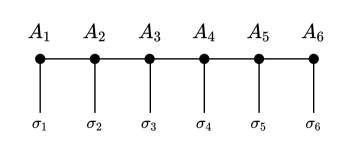
Figure 2.1: Tensor network diagram for MPS/TT (2.2). The nodes indicate tensor cores. Shared edges indicate contracted indices, while open edges indicate indices of the tensor $T(\sigma_{1},\ldots,\sigma_{6})$ represented by the diagram.

3 Decaying rank bounds

For $x\in\mathcal{D}_{K}$, which can be written uniquely as $x=\sum_{k=1}^{K}2^{-k}\sigma_{k}$, it is useful to define the component parts

$$x_{\leq m}:=\sum_{k=1}^{m}2^{-k}\sigma_{k},\quad x_{>m}:=\sum_{k=m+1}^{K}2^{-k}\sigma_{k}.$$

Note that $x_{\leq m}$ and $x_{>m}$ are arbitrary elements of $\mathcal{D}_{m}$ and $2^{-m}\,\mathcal{D}_{K-m}$, respectively, and it is useful to keep in mind the identifications

$$x_{\leq m}\leftrightarrow(\sigma_{1:m}),\quad x_{>m}\leftrightarrow(\sigma_{m+1:K}).$$

Thinking of $v\mapsto f(u+2^{-m}v)$ as a function of $v:[0,1]\rightarrow\mathbb{R}$ for fixed $u$, we can approximate it by interpolation as

$$f(u+2^{-m}v)\approx\sum_{\alpha}f(u+2^{-m}c^{\alpha})P^{\alpha}(v),$$

where $c^{\alpha}\in[0,1]$ are interpolation points (e.g., Chebyshev nodes shifted and scaled to the interval $[0,1]$), and $P^{\alpha}$ are the corresponding interpolating functions (e.g., Chebyshev cardinal functions, in the sense of [1]). Our error analysis will focus on the case of Chebyshev interpolation, but we comment that the interpolative construction that we introduce extends naturally to other interpolation schemes. In fact, in Section 4.3, we will replace ordinary Chebyshev interpolation with a notion of local Chebyshev interpolation introduced in [1], yielding significant practical speedups when the number of interpolation points is large.

Now since $f(x)=f(x_{\leq m}+x_{>m})$, we can write

$$T(\sigma_{1:K})=f(x)\approx\sum_{\alpha}\underbrace{f(x_{\leq m}+2^{-m}c^{\alpha})}_{=:T_{\mathrm{L}}^{\alpha}(\sigma_{1:m})}\underbrace{P^{\alpha}(2^{m}x_{>m})}_{=:T_{\mathrm{R}}^{\alpha}(\sigma_{m+1:K})},$$

so the $m$-th unfolding matrix $T_{m}(\sigma_{1:m},\sigma_{m+1:K})$ admits a low-rank decomposition, which in turn suggests that $T$ has low TT ranks [16]. Hence we are motivated to bound the error of Chebyshev interpolation, which is well-understood.

3.1 Notation

Before stating the technical results, we fix some notation. For any $N\geq 1$, let

$$c_{N}^{\alpha}=\frac{\cos(\pi\alpha/N)+1}{2},\quad\alpha=0,\ldots,N$$ (3.1)

denote the Chebyshev-Lobatto grid, shifted and scaled to the interval $[0,1]$. Meanwhile let $P_{N}^{\alpha}$ denote the Lagrange interpolating polynomials for these nodes, also known as the Chebyshev cardinal functions, which can be evaluated directly with simple trigonometric formulas [1].

For measuring the error of low-rank tensor decompositions it is useful to define the tensor norms

$$\|S\|_{\mathrm{\infty}}=\max_{\sigma_{1:K}\in\{0,1\}^{K}}|S(\sigma_{1:K})|,\quad\|S\|_{2}=\sqrt{\frac{1}{2^{K}}\sum_{\sigma_{1:K}\in\{0,1\}^{K}}|S(\sigma_{1:K})|^{2}}$$ (3.2)

for general $S\in\mathbb{R}^{2}\times\cdots\times\mathbb{R}^{2}$ ($K$ factors). Note that if $S$ is a quantized tensor representation for a function $g:[0,1]\rightarrow\mathbb{R}$, then our tensor 2-norm can be viewed as a Riemann sum approximation of the $L^{2}([0,1])$ norm of $g$. Observe that

$$\|S\|_{2}\leq\|S\|_{\infty}$$ (3.3)

for all $S$.

It is useful moreover to define the ordinary Frobenius norm of a tensor $\|S\|_{\mathrm{F}}$ as the ordinary Euclidean norm of its vectorization. Finally, we will use $\|\,\cdot\,\|$ to indicate the operator norm (induced by the vector Euclidean norm) of tensors when viewed as matrices as shall be clear from context.

If for $p\in\{2,\infty\}$, we define the $(\varepsilon,p)$ rank of the $m$-th unfolding matrix of $T$ to be the smallest $r$ such that

$$\left\|T-\sum_{\alpha=0}^{r-1}T_{\mathrm{L}}^{\alpha}\otimes T_{\mathrm{R}}^{\alpha}\right\|_{p}\leq\varepsilon$$

for some tensors $T_{\mathrm{L}}^{\alpha}\in(\mathbb{R}^{2})^{m}$ and $T_{\mathrm{R}}^{\alpha}\in(\mathbb{R}^{2})^{K-m}$, $\alpha=0,\ldots,r-1$. We will denote the $(\varepsilon,p)$ rank of the $m$-th unfolding matrix as $r_{m}^{(\varepsilon,p)}[T]$. Observe that $r_{m}^{(\varepsilon,2)}[T]\leq r_{m}^{(\varepsilon,\infty)}[T]$.

Finally, for every level $m$, grid size $N$, and $f:[0,1]\rightarrow\mathbb{R}$, define the polynomial interpolation error

$$E_{m,N}[f]:=\max_{u\in[0,1-2^{-m}],\,v\in[0,1]}\left|f(u+2^{-m}v)-\sum_{\alpha=0}^{N}f(u+2^{-m}c_{N}^{\alpha})P_{N}^{\alpha}(v)\right|.$$ (3.4)

Note in particular that $E_{m,N}[f]=0$ whenever $f$ is a polynomial of degree at most $N$ because $(N+1)$-point Lagrange interpolation is exact in this case.

3.2 Interpolation bound

First we state a lemma summarizing how the interpolation error (3.4) controls the ranks of the unfolding matrices.

Lemma 1.

Let $T$ be a quantized tensor representation for $f$ on $\mathcal{D}_{K}$. Let $\varepsilon>0$, and suppose that $E_{m,N}[f]\leq\varepsilon$. Then the $(\varepsilon,\infty)$ rank of the $m$-th unfolding matrix of $T$ is at most $N+1$.

Proof.

This follows directly from definitions together with the fact that $\mathcal{D}_{m}\subset[0,1-2^{-m}]$ and $\mathcal{D}_{K-m}\subset[0,1]$. ∎

Next we show how smoothness assumptions on $f$ control the interpolation error (3.4), which in turn, by the preceding lemma, controls the ranks of the unfolding matrices. The first result relies only on high-order differentiability of $f$ and is based on standard results [20] controlling Cheybhsev interpolation error.

Proposition 2.

Suppose that $f:[0,1]\rightarrow\mathbb{R}$ is $p+1$ times differentiable and that $\|f^{(p+1)}\|_{L^{\infty}([0,1])}\leq C$, where $p\geq 1$. If $N>p$, then

$$E_{m,N}[f]\leq\frac{4C}{\pi}\,\frac{2^{-m}}{p(N-p)^{p}}.$$

If $T$ is a quantized tensor representation of $f$ on $\mathcal{D}_{K}$ for $K>m$, then it follows that

$$r_{m}^{(\varepsilon,\infty)}[T]\leq 1+p+\left\lceil\left(\frac{4C}{\pi}\,\frac{2^{-m}}{p\varepsilon}\right)^{1/p}\right\rceil.$$

Remark 3.

Note that the rank bound can never drop below $p+2$, so apparently we are penalized in our bound at large depth $m$ for using high-order differentiability. Ultimately, we would like to claim that the rank drops all the way to $3$ once we reach sufficient depth $m$. Indeed, note that from the lemma it follows that if we let $C^{(q)}$ be a pointwise bound for $|f^{(q+1)}|$ for each $q=1,\ldots p$, then

$$r_{m}^{(\varepsilon,\infty)}[T]\leq 1+\left\lceil\min_{q=1,\ldots p}\left\{q+\left[\frac{2C^{(q)}}{\pi}\,\frac{2^{-m}}{q\varepsilon}\right]^{1/q}\right\}\right\rceil.$$

This rank bound satisfies $r_{m}^{(\varepsilon,\infty)}[T]\rightarrow 3$ as $m\rightarrow\infty$. A more careful argument should recover $1$ as the limiting rank, since constant interpolation is accurate at sufficiently small scales, but we will omit more detailed statements for simplicity.

The proof is given in Appendix A.

The next result is an improved bound in the case where $f$ extends analytically to a neighborhood of the interval $[0,1]$ and is again based on standard results [20] controlling Chebyshev interpolation error in this case. To state the result it is useful first to make a definition:

Definition 4.

For $\rho>1$, define the Bernstein ellipse $\mathcal{E}_{\rho}\subset\mathbb{C}$ by

$$\mathcal{E}_{\rho}:=\left\{z\in\mathbb{C}\,:\,\left[\frac{\mathrm{Re}(z)}{a_{\rho}}\right]^{2}+\left[\frac{\mathrm{Im}(z)}{b_{\rho}}\right]^{2}\leq 1\right\},$$

where

$$a_{\rho}:=\frac{\rho+\rho^{-1}}{2},\quad b_{\rho}:=\frac{\rho-\rho^{-1}}{2}.$$

Note that $\mathcal{E}_{\rho}\supset[-1,1]$, and moreover $\mathcal{E}_{\rho^{\prime}}\subset\mathcal{E}_{\rho}$ for $1<\rho^{\prime}\leq\rho$.

Proposition 5.

Suppose that for some $\rho>1$, $f:[0,1]\rightarrow\mathbb{R}$ extends analytically to $\mathcal{E}_{\rho}^{\prime}:=\frac{1}{2}\left(\mathcal{E}_{\rho}+1\right)$. Moreover suppose that there exists $B\geq 0$ such that $|f|\leq B$ on $\mathcal{E}_{\rho}^{\prime}$. Let

$$\rho_{m}:=\max\left[\rho,\,2^{m}\frac{(\rho-1)^{2}}{\rho}\right].$$

Then

$$E_{m,N}[f]\leq\frac{4B\rho_{m}^{-N}}{\rho_{m}-1}.$$

If $T$ is a quantized tensor representation of $f$ on $\mathcal{D}_{K}$ for $K>m$, then it follows that

$$r_{m}^{(\varepsilon,\infty)}[T]\leq 1+\left\lceil\log_{\rho_{m}}(1/\varepsilon)-\log_{\rho_{m}}(\rho_{m}-1)+\log_{\rho_{m}}(4B)\right\rceil.$$

Remark 6.

Consider the asymptotic rank as $m\rightarrow\infty$, in which limit $\rho_{m}=\Omega(2^{m})$. In this limit $\log_{\rho_{m}}(\rho_{m}-1)\rightarrow 1$, $\log_{\rho_{m}}(4M)\rightarrow 0$, and $\log_{\rho_{m}}(1/\varepsilon)\sim m^{-1}\log_{2}(1/\varepsilon)$. Therefore $r_{m}^{(\varepsilon,\infty)}[T]$ is roughly bounded above by $1+\lceil m^{-1}\log_{2}(1/\varepsilon)\rceil$.

The proof is also given in Appendix A.

4 Interpolative construction of QTTs

Although we have shown how smoothness quantitatively bounds the ranks of the unfolding matrices of a quantized tensor representation, we have not demonstrated an explicit construction of a QTT. In Section 4.1, we will present a direct construction based on Chebyshev interpolation using the Chebyshev-Lobatto grid $c_{N}^{\alpha}=c^{\alpha}$, where we omit $N$ from this notation going forward for visual clarity. The TT ranks in this construction are all $N+1$.

In some settings, the numerical ranks of a quantized tensor representation may be small even when a large Chebyshev-Lobatto grid is required to fully resolve the target function. The downside of our basic construction in this case is that if the quantized tensor representation has ranks much smaller than $N$, then revealing this rank via post hoc MPS/TT compression [16] would require $O(N^{3})$ operations. (For the purpose of our big-O notation, we view the depth $K$ of the network as a constant. If included, all of our big-O expressions should include an additional factor of $K$.)

Therefore in Section 4.2, we present a rank-revealing variant of the basic construction. If the true maximum TT rank (for desired error tolerance) is $r$, then this algorithm only requires $O(N^{2}r)$ operations.

Finally, in Section 4.3, we show how the dense tensor cores implementing Chebyshev interpolation can be replaced with sparse tensors, following [1], which further reduces the computational cost to $O(Nr^{2})$.

4.1 Basic construction

In the expression (2.2), fix the first tensor core $A_{1}=A_{\mathrm{L}}\in\mathbb{R}^{2\times 1\times(N+1)}$ as

$$A_{\mathrm{L}}^{1,\beta}(\sigma)=f\left(\frac{\sigma+c^{\beta}}{2}\right),\quad\beta\in[N+1],\ \sigma\in\{0,1\}.$$ (4.1)

and then for $k=2,\ldots,K-1$, fix the $k$-th tensor core $A_{k}=A\in\mathbb{R}^{2\times(N+1)\times(N+1)}$ as

$$A^{\alpha\beta}(\sigma):=P^{\alpha}\left(\frac{\sigma+c^{\beta}}{2}\right),\quad\alpha,\beta\in[N+1],\ \sigma\in\{0,1\}.$$ (4.2)

Notice that all the tensor cores $k=2,\ldots,K-1$ are exactly the same. Finally, fix the last tensor core $A_{K}=A_{\mathrm{R}}\in\mathbb{R}^{2\times(N+1)\times 1}$ as

$$A_{\mathrm{R}}^{\alpha,1}(\sigma)=P^{\alpha}\left(\frac{\sigma}{2}\right),\quad\alpha\in[N+1],\ \sigma\in\{0,1\}.$$ (4.3)

Consider the contraction of the internal tensor core with itself:

$$\left[A\cdot A\right]^{\alpha\beta}(\sigma,\tau):=\sum_{\gamma=0}^{N}A^{\alpha\gamma}(\sigma)A^{\gamma\beta}(\tau) =\sum_{\gamma=0}^{N}P^{\alpha}\left(\frac{\sigma+c^{\gamma}}{2}\right)P^{\gamma}\left(\frac{\tau+c^{\beta}}{2}\right)$$

$$=\sum_{\gamma=0}^{N}P_{\sigma}^{\alpha}\left(c^{\gamma}\right)P^{\gamma}\left(x_{\tau}^{\beta}\right),$$

where we have defined $P_{\sigma}^{\alpha}:=P^{\alpha}\left(\frac{\sigma+\,\cdot\,}{2}\right)$ and $x_{\tau}^{\beta}:=\frac{\tau+c_{N}^{\beta}}{2}$. The last expression can be viewed as a Lagrange interpolation formula for the value $P_{\sigma}^{\alpha}\left(x_{\tau}^{\beta}\right)$. However, since $P_{\sigma}^{\alpha}$ is in fact a polynomial of degree $N$, the $(N+1)$-point Lagrange interpolation is exact, and we have the exact identity

$$[A\cdot A]^{\alpha\beta}(\sigma,\tau)=P_{\sigma}^{\alpha}(x_{\tau}^{\beta})=P^{\alpha}\left(\frac{\sigma+\frac{\tau+c^{\beta}}{2}}{2}\right)=P^{\alpha}\left(\frac{\sigma}{2}+\frac{\tau}{4}+\frac{c^{\beta}}{4}\right).$$

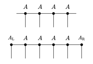
Figure 4.1: Top: tensor network diagram for the tensor $A^{p}$, where $p=4$. Bottom: the full QTT $A_{\mathrm{L}}A^{K-2}A_{\mathrm{R}}$, where $K=6$.

A straightforward inductive argument generalizes this result for arbitrary successive contractions of $A^{p}(\sigma_{1:p})=A(\sigma_{1})A(\sigma_{2})\ldots A(\sigma_{p})$ ($p$ factors) of $A$ with itself:

Lemma 7.

For any $p\geq 1$, the tensor $[A^{p}]^{\alpha\beta}(\sigma_{1:p})$, depicted graphically in Figure 4.1, satisfies

$$[A^{p}]^{\alpha\beta}(\sigma_{1:p})=P^{\alpha}\left(x_{\leq p}+2^{-p}c^{\beta}\right),$$

where $x_{\leq p}=\sum_{k=1}^{p}2^{-k}\sigma_{k}$. Moreover, the tensor $\left[A^{p}A_{\mathrm{R}}\right]^{\alpha,1}(\sigma_{1:p+1})$ satisfies

$$[A^{p}A_{\mathrm{R}}]^{\alpha}(\sigma_{1:p+1})=P^{\alpha}\left(x_{\leq p+1}\right),$$

where $x_{\leq p+1}=\sum_{k=1}^{p+1}2^{-k}\sigma_{k}$.

Proposition 8.

Let $f:[0,1]\rightarrow\mathbb{R}$, and let $T$ be its quantized tensor representation on $\mathcal{D}_{K}$. Let $A_{\mathrm{L}}$, $A$, and $A_{\mathrm{R}}$ be tensor cores defined as in (4.1), (4.2), and (4.3), respectively. The matrix product state $S:=A_{\mathrm{L}}A^{K-2}A_{\mathrm{R}}$, depicted graphically in Figure 4.1, satisfies

$$\|S-T\|_{\infty}\leq E_{1,N}[f].$$

In particular, if $f$ is a polynomial of degree at most $N$, then $S=T$.

Proof.

Note that by Lemma 7,

$$S(\sigma_{1:K}) =\sum_{\alpha=0}^{N}f\left(\frac{\sigma_{1}+c^{\alpha}}{2}\right)P^{\alpha}\left(\sum_{k=1}^{K-1}2^{-k}\sigma_{k}\right)$$

$$=\sum_{\alpha=0}^{N}f\left(x_{\leq 1}+\frac{c^{\alpha}}{2}\right)P^{\alpha}\left(2x_{>1}\right),$$

where $x_{\leq 1}=\frac{\sigma_{1}}{2}$ and $x_{>1}=\sum_{k=2}^{K}2^{-k}\sigma_{k}$. Hence $|S(\sigma_{1:K})-T(\sigma_{1:K})|\leq E_{1,N}[f]$ for all $\sigma_{1:K}$. ∎

Note that the construction of $S$ relies only on $2(N+1)$ evaluations of $f$ via the construction of $A_{\mathrm{L}}$. Meanwhile $A$ and $A_{\mathrm{R}}$ are independent of $f$.

4.2 Rank-revealing construction

The construction from the last section produces a QTT which exactly matches the Chebyshev-Lobatto interpolation of $f$ on the subintervals $[0,1/2]$ and $[1/2,1]$. In practice, the numerical TT ranks of the tensorized representation of $f$ may be smaller than the order $N$ used for polynomial approximation. (Indeed, we know from Propositions 2 and 5 that the TT ranks of the cores should decay as we move from left to right.) In principle, we can construct a QTT and then use standard MPS/TT compression algorithms to reveal the true numerical TT ranks. However, the cost of such compression is $O(N^{3})$.

In order to recover small TT ranks on the fly, we propose a rank-revealing construction with $O(N^{2}r)$ cost, where $r$ is the true maximum TT rank. The power of this approach will be further clarified in the following subsection, where sparse interpolating tensors allow us to bring the cost down further to $O(Nr^{2})$.

Suppose we have constructed $A_{\mathrm{L}}A^{p-1}$ approximately as a matrix product state $U_{1}U_{2}\cdots U_{p}R_{p}$, depicted graphically in Figure 4.2. Here the cores $U_{k}\in\mathbb{R}^{2\times r_{k-1}\times r_{k}}$, indexed as $U_{k}^{\alpha\beta}(\sigma)$, have orthonormal columns when viewed as $2r_{k-1}\times r_{k}$ matrices with respect to the index reshaping $(\sigma\alpha,\beta)$. Meanwhile, $R_{p}\in\mathbb{R}^{r_{k}\times(N+1)}$ is simply a matrix.

The first decomposition $A_{\mathrm{L}}=U_{1}R_{1}$ can be obtained by a QR decomposition of a suitable reshaping of $A_{\mathrm{L}}$. In general, we will allow for some truncation of singular values to reveal a bond dimension possible much smaller than $N$.

Inductively, given

$$A_{\mathrm{L}}A^{p-1}\approx U_{1}\cdots U_{p}R_{p},$$

we will obtain $U_{p+1}$ and $R_{p+1}$ such that $A_{\mathrm{L}}A^{p}\approx U_{1}\cdots U_{p+1}R_{p+1}$ as follows. First perform the contraction

$$B_{p}=R_{p}A\in\mathbb{R}^{2\times r_{k}\times(N+1)},\quad B_{p}^{\alpha\beta}(\sigma)=\sum_{\gamma=0}^{r_{k}-1}R_{p}^{\alpha\gamma}A^{\gamma\beta}(\sigma)$$ (4.4)

to define a new tensor $B_{p}$. Then we can view $B_{p}$ as a $2r_{k}\times(N+1)$ matrix and perform a truncated SVD with truncation rank $r_{k+1}$

$$B_{p}\approx U_{p+1}\Sigma_{p+1}V_{p+1}^{\top},\quad U_{p+1}\in\mathbb{R}^{2r_{k}\times r_{k+1}},\quad\Sigma_{p+1}\in\mathbb{R}^{r_{k+1}\times r_{k+1}},\quad V_{p+1}\in\mathbb{R}^{(N+1)\times r_{k+1}}.$$

Then $U_{p+1}$, viewed as a $2\times r_{k-1}\times r_{k}$ tensor, defines our next core, and the contraction $R_{p+1}=\Sigma_{p+1}V_{p+1}^{\top}$, which is an $r_{k+1}\times(N+1)$ matrix, completes the inductive construction.

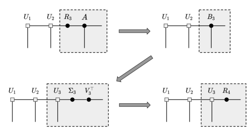
Figure 4.2: Illustration of the rank-revealing interpolative construction of QTT.

The steps of the construction for each level are depicted in Figure 4.2. In the last level (not depicted), we simply merge the outpute $R_{K}$ of the preceding step with the remaining tensor core $A_{\mathrm{R}}$, without any further truncation. For every $m=1,\ldots,K-1$, let $S_{\leq m}$ denote the tensor at the $m$-th stage of the MPS construction. Hence $S_{\leq m}$ can be viewed as an element of $\mathbb{R}^{2^{m}\times(N+1)}$. In Figure 4.2, for example, the last diagram depicts $S_{\leq 3}$.

The following result bounds the error incurred by the SVD truncations.

Theorem 9.

Let $\varepsilon>0$. In the above construction, let each SVD truncation rank $r_{k}$ be chosen as small as possible such that the Frobenius norm error of the truncation is at most $\varepsilon\sqrt{2^{k}}$. Let $S$ denote the MPS that is furnished by the construction, and let $T$ denote the true quantized tensor representation of the target function $f$. Then the total error is bounded as

$$\|T-S\|_{2}\leq E_{1,N}[f]+(K-2)\,\Lambda_{N}\,\varepsilon,$$

where $\Lambda_{N}$ is the Lebesgue constant [20] of $(N+1)$-point Chebyshev-Lobatto interpolation, which is in particular bounded by

$$\Lambda_{N}\leq 1+\frac{2}{\pi}\log(N+1).$$

Remark 10.

From the point of view of MPS/TT compression it is surprising that we can compress our tensor network at every stage of the construction because the tail $A^{p}A_{\mathrm{R}}$ of tensor cores yet to be added is not ‘isometric,’ i.e., may amplify the compression error that we make in the leading tensor indices. However, the fact that this tail of tensor cores implements Chebyshev interpolation still allows us to control the error amplification.

Proof.

We want to bound the error incurred by the successive SVD truncations. We will show that at every stage of the construction $S_{\leq m}A^{K-m-1}A_{\mathrm{R}}$ remains close to the target $T$. Accordingly, let $\varepsilon_{m}$ denote the approximation error

$$\varepsilon_{m}:=\|S_{\leq m}A^{K-m-1}A_{\mathrm{R}}-T\|_{\mathrm{F}}$$

for $m=1,\ldots,K-1$. Note that $S=S_{\leq K-1}A_{\mathrm{R}}$ is our final QTT, so $\varepsilon_{K-1}$ is the total Frobenius norm error of the construction. Meanwhile $S_{\leq 1}=A_{\mathrm{L}}$, so $\varepsilon_{1}$ is the Frobenius norm error of the uncompressed construction $A_{\mathrm{L}}A^{K-2}A_{\mathrm{R}}$, which is bounded by Proposition 8 as

$$\varepsilon_{1}\leq E_{1,N}[f]\,\sqrt{2^{K}}.$$ (4.5)

Now to bound $\varepsilon_{m}$ inductively, compute:

$$\varepsilon_{m+1} =\|T-S_{\leq m+1}A^{K-m-2}A_{\mathrm{R}}\|_{\mathrm{F}}$$

$$\leq\|T-S_{\leq m}A^{K-m-1}A_{\mathrm{R}}\|_{\mathrm{F}}+\|S_{\leq m+1}A^{K-m-2}A_{\mathrm{R}}-S_{\leq m}A^{K-m-1}A_{\mathrm{R}}\|_{\mathrm{F}}$$

$$=\varepsilon_{m}+\|(S_{\leq m+1}-S_{\leq m}A)A^{K-m-2}A_{\mathrm{R}}\|_{\mathrm{F}}$$

$$\leq\varepsilon_{m}+\|S_{\leq m+1}-S_{\leq m}A\|_{\mathrm{F}}\,\|A^{K-m-2}A_{\mathrm{R}}\|_{\mathrm{F}},$$

where we have used submultiplicativity of the Frobenius norm, applied to the product $(S_{\leq m+1}-S_{\leq m}A)A^{K-m-2}A_{\mathrm{R}}$, viewed suitably as a matrix-matrix product. Note that $\|S_{\leq m+1}-S_{\leq m}A\|_{\mathrm{F}}\leq\varepsilon\sqrt{2^{m+1}}$, precisely by construction. Therefore

$$\varepsilon_{m+1}\leq\varepsilon_{m}+\varepsilon\sqrt{2^{m+1}}\,\|A^{K-m-2}A_{\mathrm{R}}\|_{\mathrm{F}},$$ (4.6)

and it remains to bound $\|A^{K-m-2}A_{\mathrm{R}}\|_{\mathrm{F}}$.

We introduce the shorthand notation $B=A^{K-m-2}A_{\mathrm{R}}$ and view

$$B^{\alpha}(\sigma_{m+2:K}):=[A^{K-m-2}A_{\mathrm{R}}]^{\alpha}(\sigma_{m+2:K})$$

as a $2^{K-m-1}\times(N+1)$ matrix. By Lemma 7, we have that

$$B^{\alpha}(\sigma_{m+2:K})=P^{\alpha}\left(2^{m+1}\sum_{k=m+2}^{K}2^{-k}\sigma_{k}\right).$$

For further shorthand, we can write $\boldsymbol{\sigma}=\sigma_{m+2:K}\in\{0,1\}^{K-m-1}$ and write $B^{\alpha}(\boldsymbol{\sigma})=P^{\alpha}(x(\boldsymbol{\sigma}))$, where $x(\boldsymbol{\sigma})\in[0,1]$ is suitably defined as a function of $\boldsymbol{\sigma}\in\{0,1\}^{K-m-1}$.

Then

$$\|B\|_{\mathrm{F}}^{2} =\sum_{\boldsymbol{\sigma}\in\{0,1\}^{K-m-1}}\sum_{\alpha=0}^{N+1}|B^{\alpha}(\boldsymbol{\sigma})|^{2}$$

$$\leq\sum_{\boldsymbol{\sigma}\in\{0,1\}^{K-m-1}}\left(\sum_{\alpha=0}^{N+1}|B^{\alpha}(\boldsymbol{\sigma})|\right)^{2}$$

$$\leq 2^{K-m-1}\left(\sup_{x\in[0,1]}\sum_{\alpha=0}^{N+1}|P^{\alpha}(x)|\right)^{2}.$$

In fact, the quantity

$$\Lambda_{N}:=\sup_{x\in[0,1]}\sum_{\alpha=0}^{N+1}|P^{\alpha}(x)|$$

is called the Lebesgue constant of the polynomial interpolation scheme, and for the Chebyshev-Lobatto points it is known [20] that

$$\Lambda_{N}\leq 1+\frac{2}{\pi}\log(N+1).$$

In summary,

$$\|A^{K-m-2}A_{\mathrm{R}}\|_{\mathrm{F}}=\|B\|_{\mathrm{F}}\leq\Lambda_{N}\sqrt{2^{K-m-1}}.$$

Combining with (4.6), it follows that

$$\varepsilon_{m+1}\leq\varepsilon_{m}+\Lambda_{N}\,\varepsilon\sqrt{2^{K}}.$$

Then from our base bound (4.5) of $\varepsilon_{1}$, we deduce that

$$\varepsilon_{K-1}\leq\sqrt{2^{K}}\left[E_{1,N}[f]+(K-2)\,\Lambda_{N}\,\varepsilon\right].$$

Now $\|T-S\|_{2}=\sqrt{2^{-K}}\,\|T-S\|_{\mathrm{F}}=\sqrt{2^{-K}}\,\varepsilon_{K-1}$, so we conclude that

$$\|T-S\|_{2}\leq E_{1,N}[f]+(K-2)\,\Lambda_{N}\,\varepsilon,$$

as was to be shown. ∎

4.3 Sparse interpolative construction

As stated above our goal here is to improve the runtime of the interpolative construction to $O(Nr^{2})$. Observe that the $\Theta(N^{2}r)$ bottleneck in the rank-revealing construction is the construction of each core $B_{p}$ following (4.4), which requires us to perform $2(N+1)^{2}$ sums involving up to $r$ terms each, i.e., consumes $\Theta(N^{2}r)$ runtime. If the matrices $A(\sigma)$ were sparse with $O(1)$ nonzero entries per column, then the runtime would drop to $O(Nr^{2})$ as desired.

In fact, it is possible to construct sparse approximate Chebyshev interpolation matrices, up to a high order of accuracy. Our construction follows [1], and we will review the details of the construction.

Consider a function $g:[0,1]\rightarrow\mathbb{R}$. For fixed $x$, we will approximate $g(x)$ using local Lagrange interpolation on nearby Chebyshev-Lobatto nodes. As the number of local nodes used is increased, we converge stably to full Chebyshev interpolation. However, if we fix the number of local nodes and increase the underlying grid size $N$, we can obtain rapid convergence as $N$ is increased while requiring only sparse interpolation matrices.

It is more natural and effective to perform local Lagrange interpolations with respect to the angular coordinate $\theta\in[0,\pi]$, related to $x$ via $x=x(\theta)=\frac{\cos(\theta)+1}{2}$. The inverse map is denoted $\theta=\theta(x)$. Under this correspondence, the Chebyshev-Lobatto grid $c^{\alpha}$ is identified with an equispaced angular grid $\theta^{\alpha}=\frac{\alpha}{N}\pi$, $\alpha=0,\ldots,N$. To perform interpolation for a function $h(\cos(\theta))$, defined for $\theta\in[0,\pi]$ in a way that avoids boundary effects, it is useful to extend the function to the domain $\theta\in[-\pi,2\pi]$. Then one considers an extended angular grid $\theta^{\alpha}=\frac{\alpha}{N}\pi$, $\alpha=-N,\ldots,2N$. For $\gamma\in\{0,\ldots,N\}$, this extension yields the identifications $-\gamma\sim\gamma$ and $N+\gamma\sim N-\gamma$. For any $\alpha\in\{-N,\ldots,2N\}$, we let $\llbracket\alpha\rrbracket$ denote the unique representative of $\alpha$ in $\{0,\ldots,N\}$ up to this equivalence.

Now for every $\theta\in[0,\pi]$, let $\iota(\theta)$ denote the index of the closest angular grid point in $\{\theta^{\alpha}\}$. We let $M\leq N$ denote a hyperparameter which determines the order of the local Lagrange interpolation. Then we approximate $g(x)$ with its local Lagrange interpolation in the angular coordinate using interpolation points $\theta^{\gamma}$, where $\gamma=\iota(\theta)-M,\ldots,\iota(\theta)+M$. Concretely, we approximate:

$$g(x)\approx\sum_{\gamma=\iota(\theta(x))-M}^{\iota(\theta(x))+M}g(c^{\llbracket\gamma\rrbracket})\,L^{\gamma}(\theta(x)),$$ (4.7)

where

$$L^{\gamma}(\theta)=\prod_{\beta\in\{-M,\ldots,M\}\backslash\{\gamma\}}\frac{\theta-\theta^{\beta}}{\theta^{\gamma}-\theta^{\beta}}$$

are the Lagrange basis functions.

We can think of the right-hand side of (4.7) as defining a linear operator $\mathcal{I}=\mathcal{I}_{M,N}$ on the space of functions $[0,1]\rightarrow\mathbb{R}$ which sends $g$ to its interpolation $\mathcal{I}g$.

If we assume that $g$ can be approximated by an ordinary Chebyshev interpolation as

$$g\approx\sum_{\alpha=0}^{N}g(c^{\alpha})\,P^{\alpha},$$

then

$$g\approx\mathcal{I}g\approx\sum_{\alpha=0}^{N}g(c^{\alpha})\,\mathcal{I}P^{\alpha},$$ (4.8)

so we are motivated to compute

$$\mathcal{I}P^{\alpha}(x)=\sum_{\gamma=\iota(\theta(x))-M}^{\iota(\theta(x))+M}\delta^{\alpha,\llbracket\gamma\rrbracket}\,L^{\gamma}(\theta(x)),$$ (4.9)

where we have used the fact that $P^{\alpha}(c^{\beta})=\delta^{\alpha,\beta}$.

Recall moreover that in the basic construction of Section 4.1, we were interested in using evaluations $g(c^{\alpha})$ to compute the values $g\left(\frac{\sigma+c^{\beta}}{2}\right)$, for $\sigma\in\{0,1\}$, which we achieved via $g\left(\frac{\sigma+c^{\beta}}{2}\right)=\sum_{\alpha=0}^{N}g(c^{\alpha})A^{\alpha\beta}(\sigma)$. But from (4.8), we have that

$$g\left(\frac{\sigma+c^{\beta}}{2}\right)\approx\sum_{\alpha=0}^{N}g(c^{\alpha})\,\tilde{A}^{\alpha\beta}(\sigma),$$

where the tensor core $\tilde{A}\in\mathbb{R}^{2\times(N+1)\times(N+1)}$ is defined by

$$\tilde{A}^{\alpha\beta}(\sigma)=\mathcal{I}P^{\alpha}\left(\frac{\sigma+c^{\beta}}{2}\right),$$ (4.10)

where $\mathcal{I}P^{\alpha}$ is defined as in (4.9).

Observe that $\tilde{A}^{\alpha\beta}(\sigma)$ is nonzero only if

$$\left|\pi^{-1}\theta\left(\frac{\sigma+c^{\beta}}{2}\right)-\alpha\right|\leq M+1.$$

It follows that each column of $\tilde{A}(\sigma)$ has $O(M)$ nonzero entries as $N\rightarrow\infty$.

Then our sparse interpolative construction is achieved by replacing the tensor core $A$ defined in Section 4.1 with $\tilde{A}$ defined by (4.10), which depends on the additional parameter $M$ controlling the order of local interpolation. Then the rank-revealing construction of Section 4.2 is applied with $\tilde{A}$ in the place of $A$.

5 Inverting the construction

Note that the tensor $S_{\leq m}$ at stage $m$ of our construction (whether or not sparse interpolation and/or SVD truncation are applied) is an approximation of the ‘ground truth’ tensor $T_{\leq m}$ defined by

$$T_{\leq m}^{\beta}(\sigma_{1:m})=f\left(x_{\leq m}+2^{-m}c^{\beta}\right),$$

where $x_{\leq m}=\sum_{k=1}^{m}2^{-k}\sigma_{k}$, consisting of evaluations of $f$ on Chebyshev-Lobatto grids, shifted and scaled to dyadic subintervals of $[0,1]$.

It is natural to ask whether it is possible to ‘invert’ our construction to recover such evaluations from a given QTT for a function $f$, which only directly furnishes evaluations of $f$ on the dyadic grid $\mathcal{D}_{K}$. This can be achived in two stages:

1. Recover evaluations of $f$ on small-scale Chebyshev-Lobatto grids using Lagrange interpolation on small-scale equispaced grids.

2. Recover $f$ on larger scale Chebyshev-Lobatto grids from finer Chebyshev-Lobatto grids by Chebyshev interpolation.

To accomplish the first stage, consider the Lagrange interpolating polynomials on a small-scale dyadic grid $\mathcal{D}_{q}\subset[0,1]$, which we evaluate on the Chebyshev-Lobatto grid $\{c^{\beta}\}\subset[0,1]$. The dyadic grid points in $\mathcal{D}_{q}$ can be written $\sum_{k=1}^{q}2^{-k}\sigma_{k}$, indexed by $\sigma_{1:q}\in\{0,1\}^{q}$, which motivates us to define the Lagrange interpolation tensor $L\in\mathbb{R}^{2^{q}\times(N+1)}$

$$L^{\beta}(\sigma_{1:q})=\prod_{\tau_{1:q}\in\{0,1\}^{q}\backslash\{\sigma_{1:q}\}}\frac{c^{\beta}-\sum_{k=1}^{q}2^{-k}\tau_{k}}{\sum_{k=1}^{q}2^{-k}(\sigma_{k}-\tau_{k})}.$$

$L$ can be contracted with $S$, as indicated at the top of Figure 5.1, to obtain an approximation $S_{\leq K-q}$ for $T_{\leq K-q}$. The expression for this contraction is written

$$S_{\leq K-q}^{\beta}(\sigma_{1:K-q})=\sum_{\sigma_{K-q+1:K}\in\{0,1\}^{q}}S(\sigma_{1:K})\,L^{\beta}(\sigma_{K-q+1:K}).$$

Due to Runge’s phenomenon, it is not safe to take $q$ large while the depth $K$ is fixed. However, since the conceit of QTT is that the depth $K$ can be taken large enough to resolve all the fine-scale structure of the target function $f$, even Lagrange interpolation with a fixed small value of $q$ will be very accurate. For smooth functions, the error will be exponentially small in $K$ for fixed $q$, with more rapid asymptotic convergence in $K$ when $q$ is larger. For many concrete purposes, $q=1$ should suffice. We will not make any explicit careful statement, though standard Lagrange error bounds can be consulted.

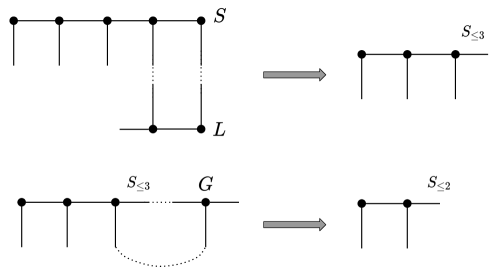
Figure 5.1: Top: stage 1 of the inversion procedure. Bottom: one level of stage 2.

Now we turn to stage 2 of the inversion procedure. To inductively obtain $S_{\leq k}$ from $S_{\leq k+1}$, we want to invert the operation of tacking on a single tensor core $A$. Accordingly, we want to define a tensor $G\in\mathbb{R}^{2\times(N+1)\times(N+1)}$, indexed as $G^{\alpha\beta}(\sigma)$, such that

$$\sum_{\sigma\in\{0,1\}}\sum_{\gamma=0}^{N}A^{\alpha\beta}(\sigma)G^{\beta\gamma}(\sigma)=\delta^{\alpha\gamma},$$ (5.1)

i.e., we seek $G$ which is a generalized inverse of $A$, viewed appropately as a matrix of shape $2(N+1)\times(N+1)$.

This problem is underdetermined, but there exists a solution $G$ whose entries remain bounded as the interpolation grid size $N$ becomes large:

$$G^{\alpha\beta}(\sigma)=\begin{cases}\delta_{\sigma 0}P^{\alpha}\left(2c^{\beta}\right),&c^{\beta}\in[0,1/2]\\ \delta_{\sigma 1}P^{\alpha}(2c^{\beta}-1),&c^{\beta}\in(1/2,1].\end{cases}$$ (5.2)

Note that by construction $|G^{\alpha\beta}(\sigma)|\leq 1$ for all $\alpha,\beta,\sigma$.

Lemma 11.

The tensor core $G$ as defined in (5.2) satisfies the inversion property (5.1). Moreover, all entries of $G$ are bounded by $1$ in absolute value.

Proof.

It remains only to verify the inversion property. Compute:

$$\sum_{\sigma\in\{0,1\}}\sum_{\beta=0}^{N}A^{\alpha\beta}(\sigma)G^{\beta\gamma}(\sigma)=\begin{cases}\sum_{\beta=0}^{N}A^{\alpha\beta}(0)G^{\beta\gamma}(0),&c^{\gamma}\in[0,1/2],\\ \sum_{\beta=0}^{N}A^{\alpha\beta}(1)G^{\beta\gamma}(1),&c^{\gamma}\in(1/2,1].\end{cases}$$

Note that for either $\sigma\in\{0,1\}$,

$$\sum_{\beta=0}^{N}A^{\alpha\beta}(\sigma)G^{\beta\gamma}(\sigma) =\sum_{\beta}P^{\alpha}\left(\frac{\sigma+c^{\beta}}{2}\right)P^{\beta}(2c^{\gamma}-\sigma)$$

$$=P^{\alpha}\left(\frac{\sigma+(2c^{\gamma}-\sigma)}{2}\right)$$

$$=P^{\alpha}(c^{\gamma})$$

$$=\delta^{\alpha\gamma},$$

where we have used the fact that $(N+1)$-point polynomial interpolation of the degree-$N$ polynomial $P^{\alpha}\left(\frac{\sigma+\,\cdot\,}{2}\right)$ is exact. ∎

6 Multiresolution interpolative construction

So far our interpolative construction depends only evaluations of the target function $f$ on a single coarse grid $\frac{\sigma+c^{\alpha}}{2}$, $\sigma\in\{0,1\}$, $\alpha=0,\ldots,N$. In this construction we must take $N$ large enough to resolve all the features of $f$, as we have quantified in Proposition 8. It can be observed empirically, however, that certain functions, which may even be nonsmooth, have low QTT ranks even though they cannot be interpolated from a single coarse grid.

In this section, we explain this behavior and provide a direct construction that achieves low TT ranks using additional a priori knowledge. We comment that a rank-revealing construction using sparse interpolation, as outlined in Sections 4.2 and 4.3, may still be adequate for the practical purpose of compressing some target function $f$.

Suppose that at each level $k<K$, we are given a collection $\mathcal{S}_{k}$ of multi-indices $\sigma_{1:k}^{i}=(\sigma_{1}^{i},\ldots,\sigma_{k}^{i})$, where $i=1,\ldots,q_{k}$. Concretely:

$$\mathcal{S}_{k}=\left\{\sigma_{1:k}^{i}\,:\,i=1,\ldots,q_{k}\right\}.$$

For each $i$, let

$$x_{\leq k}^{i}=\sum_{l=1}^{k}2^{-l}\sigma_{l}$$

denote the dyadic grid point corresponding to $\sigma_{1:k}$. By convention we take $\mathcal{S}_{K}=\emptyset$.

We will think of the dyadic subintervals $[x_{\leq k}^{i},x_{\leq k}^{i}+2^{-k}]$ as a collection of ‘dangerous’ subintervals on which the sharp behavior of $f$ makes it too dangerous to interpolate. Within these subintervals, we defer function evaluation.

Importantly, we assume that each $\sigma_{1:k+1}^{i}\in\mathcal{S}_{k+1}$ can be written as $(\sigma_{1:k}^{j},\sigma)$ for some $\sigma_{1:k}^{j}\in\mathcal{S}_{k}$ and $\sigma\in\{0,1\}$. In other words, each dangerous subinterval is contained within a dangerous subinterval at the next largest scale.

For example, consider a function such as $f(x)=\sqrt{x}$, with a cusp at the left endpoint of the interval $[0,1]$. In this case it will be effective to take $q_{k}=1$ and $\sigma_{1:k}^{1}=(0,0,\ldots,0)$ for each $k$. Accordingly, we view the subintervals $[0,2^{-k}]$ as dangerous, but all other dyadic subintervals, such as $[2^{-k},2^{-k}+2^{-m}]$ for $m\geq k$, are viewed as safe.

We illustrate a choice of subintervals for a function with a cusp in Figure 6.1.

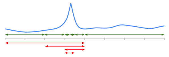
Figure 6.1: Consider a function with a single cusp, whose graph is indicated by the blue line. The red intervals indicate our choice of ‘dangerous’ subintervals at each level of resolution. The resulting QTT with $K=4$ will perform exact Chebyshev-Lobatto interpolation using function evaluations on the subintervals indicated in green.

Our inductive target for the QTT construction is the tensor $T_{\leq k}\in\mathbb{R}^{2^{k}\times(N+1+q_{k})}$ defined by stacking two tensors $T_{\leq k}^{\,\mathrm{up}}\in\mathbb{R}^{2^{k}\times(N+1)}$ and $T_{\leq k}^{\,\mathrm{down}}\in\mathbb{R}^{2^{k}\times q_{k}}$, where

$$\left[T_{\leq k}^{\,\mathrm{up}}\right]^{\beta}(\sigma_{1:k})=\begin{cases}f\left(x_{\leq k}+2^{-k}c^{\beta}\right),&\sigma_{1:k}\notin\mathcal{S}_{k},\\ 0,&\text{otherwise},\end{cases}$$

and

$$\left[T_{\leq k}^{\,\mathrm{down}}\right]^{i}(\sigma_{1:k})=\begin{cases}1,&\sigma_{1:k}=\sigma_{1:k}^{i},\\ 0,&\text{otherwise}.\end{cases}$$

Thus $T_{\leq k}(\sigma_{1:k})$ stores several pieces of information. First, it tells us whether or not we are in a dangerous interval. In this case, the top part of the vector is the zero vector, and the bottom part is an indicator vector telling us which dangerous subinterval we are in. Second, it tells us, if we are in a safe interval, the function values that we will need to interpolate the function on this interval.

We need to determine the tensor core $A_{k}$ (extending the core $A$ introduced in Section 4.1), that can be attached to $T_{\leq k}$ to obtain $T_{\leq k+1}$ approximately. This tensor can be defined in a block sense as

$$A_{k}(\sigma)=\left(\begin{array}[]{cc}A(\sigma)&0\\ F_{k}(\sigma)&\chi_{k}(\sigma)\end{array}\right).$$

Here the entire matrix is $(N+1+q_{k-1})\times(N+1+q_{k})$ and the upper-left block is $(N+1)\times(N+1)$. The lower blocks are defined as

$$F_{k}^{i\beta}(\sigma)=\begin{cases}0,&(\sigma_{k-1}^{i},\sigma)\in\mathcal{S}_{k},\\ f(x_{\leq k-1}^{i}+2^{-k}\sigma+2^{-k}c^{\beta}),&\text{otherwise},\end{cases}$$

and

$$\chi_{k}^{ij}(\sigma)=\begin{cases}1,&\sigma_{1:k}^{j}=(\sigma_{1:k-1}^{i},\sigma),\\ 0,&\text{otherwise}.\end{cases}$$

For the initial tensor core, we can simply take $A_{1}=T_{\leq 1}$ directly. For the final tensor core, define

$$A_{K}(\sigma)=\left(\begin{array}[]{c}A_{\mathrm{R}}(\sigma)\\ F_{K}(\sigma)\end{array}\right),$$

where

$$F_{K}^{i,1}(\sigma)=f(x_{\leq K-1}^{i}+2^{-K}\sigma).$$

The entire QTT is constructed as $S:=A_{1}A_{2}\cdots A_{K}$, which is shorthand for (2.2). Careful inspection reveals the following interpretation of the entries $S(\sigma_{1:K})$:

Theorem 12.

The QTT $S$ constructed following the above procedure admits the following interpretation. For fixed $\sigma_{1:K}$, consider the smallest $k$ such that $\sigma_{1:k}\notin\mathcal{S}_{k}$. If $k\leq K-1$, then

$$S(\sigma_{1:K})=\sum_{\alpha=0}^{N}f(x_{\leq k}+2^{-k}c^{\alpha})\,P^{\alpha}(2^{k}x_{>k}),$$

where $x_{\leq k}=\sum_{l=1}^{k}2^{-l}\sigma_{l}$ and $x_{>k}=\sum_{l=k+1}^{K}2^{-l}\sigma_{l}$. In other words, the value $S(\sigma_{1:K})$ is furnished in this case by interpolation of $f$, evaluated at the point $x_{\leq K}$, using a Chebyshev-Lobatto grid shifted and scaled to the interval $\left[x_{\leq k},x_{\leq k}+2^{-k}\right]$. Meanwhile, if $k=K$, then $S(\sigma_{1:K})$ is furnished by the exact evaluation $f(x_{\leq K})$.

Letting $T$ denote the exact quantized tensor representation of $f$, it follows that

$$\|S-T\|_{\infty}\leq\max\left\{E_{I,N}[f]\ :I\notin\bigcup_{k=1}^{K-1}\mathcal{S}_{k}\ \text{is a dyadic subinterval of}\ [0,1]\ \text{of length at least }2^{-(K-1)}\right\}.$$

In the last expression, the dyadic subintervals are the intervals of the form $[x,x+2^{-k}]$ where $x\in\mathcal{D}_{k}$ and $k\in\{1,\ldots,K-1\}$, and $E_{I,N}[f]$ denotes the $L^{\infty}$-norm error of $(N+1)$-point Chebyshev-Lobatto interpolation of $f$ on the interval $I$.

Using this error bound, it is simple to derive a priori bounds for the compression of certain functions. For example, consider the function $f(x)=\sqrt{x}$ with the subinterval selection indicated above—i.e., $q_{k}=1$ and $\sigma_{1:k}^{1}=(0,0,\ldots,0)$ for each $k=1,\ldots,K-1$. The ‘worst’ subintervals where we need to control the interpolation are the subintervals $[2^{-k},2^{1-k}]$, $k=1,\ldots,K-1$. In fact, $f$ is self-similar on this collection of intervals, and the worst of these is the case $k=1$ (since the restrictions of $f$ to all the other intervals, rescaled to the same domain $[1/2,1]$ are scalar multiples with decaying prefactors). Hence we are motivated to bound $(N+1)$-point Chebyshev-Lobatto interpolation error of $f(x)=\sqrt{x}$ on the interval $[1/2,1]$. In turn we are motivated to bound the interpolation error of $g(x)=\frac{1}{2}\sqrt{x+3}$ on the reference interval $[-1,1]$. Now $g$ extends analytically to the Bernstein ellipse $\mathcal{E}_{\rho}$ for $\rho\in[1,3+2\sqrt{2}]$ and is bounded by $M_{\rho}=\frac{1}{2}\sqrt{\frac{\rho+\rho^{-1}}{2}+3}$ on this region. Consider the extreme choice $\rho=3+2\sqrt{2}$, yielding $M_{\rho}=\frac{\sqrt{6}}{2}$, so by applying Theorem 8.2 of [20] (cf. the proof Proposition 5) we have that the interpolation error is bounded by

$$\frac{2\sqrt{6}\rho^{-N}}{\rho-1}\leq(1.015)\times(5.828)^{-N}.$$

7 Multivariate functions

Several approaches have been considered for extending the use of quantized tensor trains to multivariate functions; see for instance [23, 22].

We review the main ideas of the multivariate setting. Considering a function $f:[0,1]^{d}\rightarrow\mathbb{R}$, we now place the vector variable $\boldsymbol{x}\in[0,1]^{d}$ in bijection with sequences of the form $\boldsymbol{\sigma}_{1},\boldsymbol{\sigma}_{2},\ldots$, where $\boldsymbol{\sigma}_{k}=(\sigma_{k1},\ldots\sigma_{kd})\in\{0,1\}^{d}$ for each $k$, using the identification

$$\boldsymbol{x}=\sum_{k=1}^{\infty}2^{-k}\boldsymbol{\sigma}_{k}=\left(\begin{array}[]{c}0.\sigma_{11}\sigma_{21}\sigma_{31}\cdots\\ 0.\sigma_{12}\sigma_{22}\sigma_{32}\cdots\\ \vdots\\ 0.\sigma_{1d}\sigma_{2d}\sigma_{3d}\cdots\end{array}\right),$$ (7.1)

where the entries in the expression at right indicate binary decimal expansions for each of the components of $\boldsymbol{x}$.

We choose a depth $K$ at which to truncate the decimal expansion, so the identification

$$\boldsymbol{x}\leftrightarrow(\boldsymbol{\sigma}_{1},\ldots,\boldsymbol{\sigma}_{K})$$

is a bijection between the dyadic grid $\mathcal{D}_{K}^{d}=\left(2^{-K}\,\mathbb{Z}^{d}\right)\cap[0,1)^{d}$ and the set $\{0,1\}^{d}\times\cdots\times\{0,1\}^{d}$, where the direct product includes $K$ factors. Based on this identification, we can in turn identify functions $f:\mathcal{D}_{K}^{d}\rightarrow\mathbb{R}$ with tensors $T\in\mathbb{R}^{2^{d}}\times\cdots\times\mathbb{R}^{2^{d}}$ via

$$f(\boldsymbol{x})=T(\boldsymbol{\sigma}_{1},\ldots,\boldsymbol{\sigma}_{d}).$$

Such a tensor could be compressed as a tensor train where the external dimension of each core is $2^{d}$. However, it is typical not to take this course but instead to further split each $\boldsymbol{\sigma}_{k}=(\sigma_{k1},\ldots\sigma_{kd})$ into its component parts to allow for the possibility of additional compression.

Accordingly we can $f$ as a tensor via either

$$f(\boldsymbol{x})=T(\underbrace{\sigma_{11},\sigma_{12},\ldots,\sigma_{1d}}_{\text{depth 1}},\,\underbrace{\sigma_{21},\sigma_{22},\ldots,\sigma_{2d}}_{\text{depth 2}},\,\ldots,\underbrace{\sigma_{K1},\sigma_{K2},\ldots,\sigma_{Kd}}_{\text{depth K}})$$ (7.2)

or

$$f(\boldsymbol{x})=T(\underbrace{\sigma_{11},\sigma_{21},\ldots,\sigma_{K1}}_{\text{variable 1}},\,\underbrace{\sigma_{12},\sigma_{22},\ldots,\sigma_{K2}}_{\text{variable 2}},\,\ldots,\underbrace{\sigma_{1d},\sigma_{2d},\ldots,\sigma_{Kd}}_{\text{variable d}}).$$ (7.3)

In the first representation (7.2), the bits $\sigma_{ki}$ are organized first by depth index $k$ and then by variable index $i$. In the second representation (7.3), they are organized first by variable and then by depth.

Typically (7.2) is referred to as the interleaved ordering, while (7.3) is referred to as the serial ordering. (However, we comment that the naming convention depends on a matter of perspective.) In the following we explain how our construction generalizes to both of these orderings.

7.1 Interleaved ordering

For simplicity of presentation, we will explicitly consider the case where $\boldsymbol{x}=(x,y,z)\in\mathbb{R}^{3}$, i.e., $d=3$.

Here the left core $A_{\mathrm{L}}^{x}\in\mathbb{R}^{2\times 1\times(N+1)^{3}}$ is defined by

$$\left[A_{\mathrm{L}}(\sigma)\right]^{1,\beta_{x}\beta_{y}\beta_{z}}=f\left(\frac{\sigma+c^{\beta_{x}}}{2},c^{\beta_{y}},c^{\beta_{z}}\right),\quad\beta_{x},\beta_{y},\beta_{z}\in[N+1],\ \sigma\in\{0,1\}.$$ (7.4)

Then with the univariate interpolating tensor core $A\in\mathbb{R}^{2\times(N+1)\times(N+1)}$ defined as in (4.2), we define interpolating tensor cores $A^{x},A^{y},A^{z}\in\mathbb{R}^{2\times(N+1)^{3}\times(N+1)^{3}}$ for the $x$, $y$, and $z$ dimensions as

$$A^{x}(\sigma)=A(\sigma)\otimes I_{N+1}\otimes I_{N+1},\quad A^{y}(\sigma)=I_{N+1}\otimes A(\sigma)\otimes I_{N+1},\quad A^{z}(\sigma)=I_{N+1}\otimes I_{N+1}\otimes A(\sigma).$$ (7.5)

Observe that appending the tensor core $A^{x}$ from the right, for example, performs Chebyshev interpolation in the $x$ dimension.

Finally the tensor train is capped off with cores $A_{\mathrm{R}}^{x}\in\mathbb{R}^{2\times(N+1)^{3}\times(N+1)^{2}}$, $A_{\mathrm{R}}^{y}\in\mathbb{R}^{2\times(N+1)^{2}\times(N+1)}$, $A_{\mathrm{R}}^{z}\in\mathbb{R}^{2\times(N+1)\times 1}$ given by

$$A_{\mathrm{R}}^{x}(\sigma)=A_{\mathrm{R}}(\sigma)\otimes I_{N+1}\otimes I_{N+1},\quad A_{\mathrm{R}}^{y}(\sigma)=A_{\mathrm{R}}(\sigma)\otimes I_{N+1},\quad A_{\mathrm{R}}^{z}(\sigma)=A_{\mathrm{R}},$$ (7.6)

where $A_{\mathrm{R}}$ is defined as in (4.3). The overall construction is illustrated in Figure 7.1.

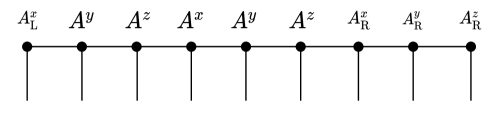
Figure 7.1: Interpolative multivariate QTT construction in the interleaved ordering.

It is straightforward to extend the rank-revealing construction of Section 4.2 to this setting by successively performing SVDs in the same fashion. Note that due to the tensor product structure, matrix-vector multiplication by the matrices $A^{x}(\sigma),A^{y}(\sigma),A^{z}(\sigma)$ can be achieved in $O(N^{4})$ time. In the general $d$-dimensional setting, the scaling of these matvecs is $O(N^{d+1})$. Therefore if the revealed rank is $r$, then the cost of this construction is only $O(N^{d+1}r^{2})$.

It also automatic to extend the sparse interpolative construction of Section 4.3 to this setting by simply replacing the dense tensor core $A(\sigma)$ with its sparse counterpart. Then we can obtain $O(N^{d}r^{2})$ complexity in the rank-revealing construction.

It is also possible to extend the construction of Section 6 for resolving sharp features, by choosing a collection of nested dyadic rectangles.

7.2 Serial ordering

Again for concreteness we will explicitly consider the case where $\boldsymbol{x}=(x,y,z)\in\mathbb{R}^{3}$, i.e., $d=3$.

For QTT construction in serial ordering, we will make use of the tensor cores $A_{\mathrm{L}}$, $A^{x}$, $A_{\mathrm{R}}^{x}$, $A_{\mathrm{R}}^{y}$, and $A_{\mathrm{R}}^{z}$, defined before in equations (7.4), (7.5), and (7.6). However, the tensors $A^{y}$ and $A^{z}$ defined above are not directly suitable, so we also define

$$\hat{A}^{y}(\sigma)=A(\sigma)\otimes I_{N+1},\quad\hat{A}^{z}(\sigma)=A(\sigma).$$

Here although simply $\hat{A}^{z}=A$, we opt for the suggestive notation. The construction in serial ordering can be viewed as interpolating in the $x$ variable to full depth, then capping off this interpolation and interpolating in the $y$ variable to full depth, etc. This procedure is illustrated in Figure 7.2.

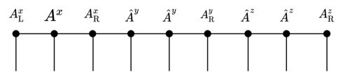
Figure 7.2: Interpolative multivariate QTT construction in the serial ordering.

The rank-revealing and sparse constructions of Sections 4.2 and 4.3 can be extended here to yield cost scalings of $O(N^{d+1}r^{2})$ and $O(N^{d}r^{2})$, respectively.

However, we comment that it is not obvious how to extend the multiresolution construction of Section 6 to this setting.

8 Numerical experiments

In this section we present several illustrative numerical experiments.

8.1 Dense interpolation

Consider the function $f:[0,1]\rightarrow\mathbb{R}$ defined by

$$f(x)=\sum_{j=1}^{J}\left[a_{j}\cos(2\pi jx)+b_{j}\sin(2\pi jx)\right],$$ (8.1)

where the $a_{j},b_{j}$ are independently distributed standard normal random variables.

First we fix one typical instantiantiation of this function with $J=25$. In Figure 8.1, we present the accuracies of both our basic interpolative construction and tensor cross interpolation (implemented as amen_cross in the TT-Toolbox package [14]) against the number of function evaluations required by each method. Note that the construction of Section 4.1 requires $2N+1$ function evaluations. The figure demonstrates the significant advantage of the first approach.

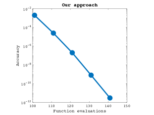
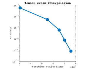
Figure 8.1: Error of our basic interpolative construction (left) and tensor cross interpolation (right) for (8.1) with $J=25$, plotted against the number of function evaluations. Error is measured by the infinity norm on the dyadic grid $\mathcal{D}_{20}$. Note the different scales of the horizontal axes.

When $J$ becomes larger than about $100$, as the function becomes highly oscillatory, tensor cross interpolation (TCI) fails to converge, while our interpolative construction remains stable. We show in Figure 8.2 that our accuracy remains roughly fixed if we scale $N=\Omega(J)$.

$J$	200	300	400	500	600	1000	2000
Error	$9.8\times 10^{-11}$	$1.1\times 10^{-10}$	$8.4\times 10^{-11}$	$1.3\times 10^{-10}$	$1.8\times 10^{-10}$	$2.2\times 10^{-10}$	$3.5\times 10^{-10}$

Figure 8.2: Error of our approach for (8.1) as a function of $J$, where we take $N=2J$. Error is measured by the infinity norm on the dyadic grid $\mathcal{D}_{20}$. Note that tensor cross interpolation fails to converge for these examples.

8.2 Sparse interpolation

For $\alpha>0$, consider the function

$$f(x)=\frac{\alpha}{\sqrt{\alpha^{2}+(x-1/2)^{2}}},$$ (8.2)

which is peaked at $x=1/2$. The peak becomes increasingly sharp as $\alpha\rightarrow 0$. However (cf. Section 6), the TT ranks of $f$ remain roughly constant in this limit.

We will demonstrate that the sparse and rank-revealing interpolation scheme of Section 4.3 can be applied effectively to this function in the large $N$ limit. (Of course, the approach of Section 6 could well be applied here given a priori knowledge about the peak location.)

In order to maintain fixed accuracy, we must scale $N$ with $\alpha$ as $N\sim C/\sqrt{\alpha}$. Alternatively, we can consider $\alpha$ as a function of $N$, for several different fixed values of $C$. In Figure 8.3 we plot the error of our sparse interpolation scheme. Given the necessary function evaluations, each construction in the figure was completed in less than 0.5 seconds on a 2021 M1 MacBook Pro, which would not be possible of $\Omega(N^{3})$ or even $\Omega(N^{2})$ operations were required.

            

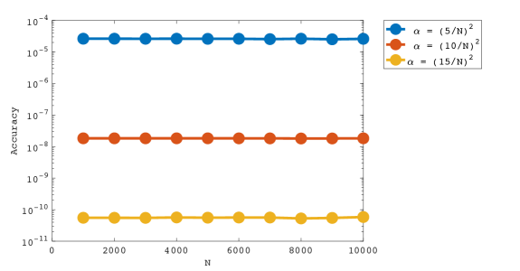
Figure 8.3: Error of our approach for (8.2) where we scale $\alpha$ with $N$ according to the legend. Error is measured by the infinity norm on the dyadic grid $\mathcal{D}_{25}$.

8.3 Inverting the construction

Consider (8.2) once again where we now fix the value $\alpha=0.1$. We will use this example to validate the ‘inversion’ algorithm of Section 5. We choose $N=300$, more than large enough to ensure machine precision of our QTT.

For the inverse construction, we simply take $q=1$, so the local Lagrange interpolation is linear, which is accurate up to error $O(h^{2})$ on an interval of size $O(h)$. Therefore we expect that as the depth $K$ is increased, the accuracy of our inversion algorithm should scale as $(2^{-K})^{2}=2^{-2K}$. To measure this accuracy, we use the algorithm of Section 5 to recover the evaluations $f(c^{\alpha}/2)$, $\alpha=0,\ldots,N$, and we record the worst case error over $\alpha$ of the recovery. The results are plotted in Figure 8.4, and they validate our scaling prediction.

                  

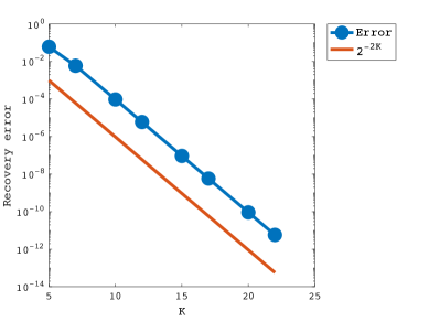
Figure 8.4: Worst-case error of the recovery of $f(c^{\alpha}/2)$ from a QTT for $f$ (following the algorithm of Section 5), plotted against the depth $K$.

8.4 Multiresolution construction

Next consider the Gaussian function

$$f(x)=e^{-\frac{1}{2}(x/\alpha)^{2}}.$$ (8.3)

In [3] a bound for the QTT ranks of $f$ was provided based on approximation with Fourier series, but this rank bound is not uniform with respect to the scale $\alpha$ of the Gaussian function. In particular, in the limit $\alpha\rightarrow 0$, the quantitative smoothness of $f$ deteriorates. Nevertheless, it may be observed empirically that the QTT ranks of $f$ are bounded independently of $\alpha$. Our multiresolution construction of Section 6 clarifies this phenomenon, and here we validate this perspective with numerics.

Fix $K=25$, and adopt the subintervals considered above in our discussion of the function $f(x)=\sqrt{x}$ (cf. Section 6), i.e., take $q_{k}=1$ and $\sigma_{1:k}^{1}=(0,0,\ldots,0)$ for all $k=1,\ldots,K-1$. In Figure 8.5, we plot the error of the multiresolution construction of Section 6 as a function of $\alpha$ for several values of $N$. Observe that uniformly bounded error is achieved in the limit $\alpha\rightarrow 0$, and in fact machine precision across all $\alpha$ is already almost attained by $N=18$.

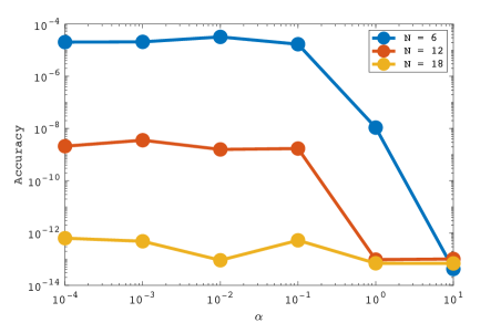
Figure 8.5: Error of the multiresolution construction for (8.3) as a function of $\alpha$, for several values of $N$ indicated by the legend. Error is measured by the infinity norm on the dyadic grid $\mathcal{D}_{25}$.

8.5 Multivariate construction

Finally we simply demonstrate the application of the multivariate construction in the serial ordering (cf. Section (7.2)) to the bivariate function

$$f(x,y)=\frac{1}{1+100\left[(x-1/2)^{2}+(y-1/2)^{2}\right]}.$$ (8.4)

We fix $K=10$ and plot the error as a function of $N$ in Figure 8.6.

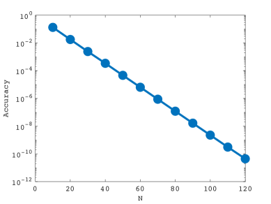
Figure 8.6: Error of the multivariate construction in the serial ordering (cf. Section (7.2)) for the function (8.4) as a function of $N$. Error is measured by the infinity norm on the dyadic grid $\mathcal{D}_{10}^{2}$.

Appendix A     Proofs of interpolation bounds

In this section we prove the interpolation bounds of Section 3.2.

Proof of Proposition 2..

The bound on $E_{m,N}[f]$ follows directly from the interpolation error bound of Theorem 7.2 of [20], which bounds the pointwise interpolation error of a function $g:[-1,1]\rightarrow\mathbb{R}$ (using a suitable Chebyshev-Lobatto grid) by

$$\frac{4V}{\pi p(N-p)^{p}},$$

where $V$ is the total variation of $g^{(p)}$.

The only wrinkle is that we need to shift and scale the functions that we want to interpolate to the reference interval $[-1,1]$. At level $m$, for any fixed $u\in[0,1-2^{-m}]$, we want to interpolate the function $g_{m,u}(x):=f\left(u+2^{-m}\left[\frac{x+1}{2}\right]\right)$ defined on the domain $x\in[-1,1]$. Since $g_{m,u}^{(p)}$ is differentiable by assumption, the total variation of $g_{m,u}^{(p)}$ is equal to

$$\|g_{m,u}^{(p+1)}\|_{L^{1}([-1,1])}\leq 2\|g_{m,u}^{(p+1)}\|_{L^{\infty}([-1,1])}.$$

But $g_{m,u}^{(p+1)}(x)=2^{-(m+1)}f^{(p+1)}\left(u+2^{-m}\left[\frac{x+1}{2}\right]\right)$, so

$$\|g_{m,u}^{(p+1)}\|_{L^{\infty}([-1,1])}\leq 2^{-(m+1)}\|f^{(p+1)}\|_{L^{\infty}([0,1])}\leq 2^{-(m+1)}C,$$

and it follows that the total variation of $g_{m,u}^{(p)}$ is bounded by $2^{-m}C$. This concludes the proof. ∎

Proof of Proposition 5..

The bound on $E_{m,N}[f]$ follows directly from the interpolation error bound of Theorem 8.2 of [20], which states that if $g:[-1,1]\rightarrow\mathbb{R}$ extends analytically to $\mathcal{E}_{\rho}$ and $|g|\leq M$ on $\mathcal{E}_{\rho}$, then the pointwise interpolation error for $g$ using Chebyshev-Lobatto grid of size $N$ is bounded by

$$\frac{4M\rho^{-N}}{\rho-1}.$$

At level $m$, for any fixed $u\in[0,1-2^{-m}]$, we want to interpolate the function $g_{m,u}(x):=f\left(u+2^{-m}\left[\frac{x+1}{2}\right]\right)$ defined on the domain $x\in[-1,1]$. Hence we are motivated to consider the question: for which values of $\rho^{\prime}>1$ does the containment

$$u+2^{-m}\left[\frac{\mathcal{E}_{\rho^{\prime}}+1}{2}\right]\subset\frac{\mathcal{E}_{\rho}+1}{2}$$

hold? Equivalently, we ask for the containment

$$\left(2u-1+2^{-m}\right)+2^{-m}\mathcal{E}_{\rho^{\prime}}\subset\mathcal{E}_{\rho}.$$

Note that the extreme values for $2u-1+2^{-m}$ (over all allowed values $u$) are $\pm(1-2^{-m})$. Therefore it will suffice to ask for

$$(1-2^{-m})+2^{-m}\mathcal{E}_{\rho^{\prime}}\subset\mathcal{E}_{\rho}.$$

In turn, for this containment of ellipses to hold it suffices that the following inequalities hold for their semi-major axes:

$$(1-2^{-m})+2^{-m}a_{\rho^{\prime}}\leq a_{\rho},\quad 2^{-m}b_{\rho^{\prime}}\leq b_{\rho},$$

which finally lead to the desiderata

$$a_{\rho^{\prime}}\leq 2^{m}\left(a_{\rho}-1\right)+1,\quad b_{\rho^{\prime}}\leq 2^{m}b_{\rho}.$$

First we observe that these inequalities always hold trivially if we take $\rho^{\prime}=\rho$. However, asymptotically as $m\rightarrow\infty$, we will see that we can achieve far larger $\rho^{\prime}=\Omega(2^{m})$.

Indeed, observe that for all $r\geq 1$, $a_{r}=\frac{r+r^{-1}}{2}$ and $b_{r}=\frac{r-r^{-1}}{2}$ satisfy the inequalities

$$\frac{r}{2}\leq a_{r}\leq\frac{r+1}{2},\quad\frac{r-1}{2}\leq b_{r}\leq\frac{r}{2}.$$

Therefore it suffices that

$$\rho^{\prime}\leq 2^{m+1}\left(a_{\rho}-1\right)+1,\quad\rho^{\prime}\leq 2^{m}(\rho-1).$$

In fact, $a_{\rho}-1\leq\frac{\rho-1}{2}$ for $\rho\geq 1$, so both conditions are implied by the stronger inequality

$$\rho^{\prime}\leq 2^{m+1}(a_{\rho}-1)=2^{m}\frac{(\rho-1)^{2}}{\rho}.$$

Therefore if we take

$$\rho_{m}:=\max\left[\rho,\,2^{m}\frac{(\rho-1)^{2}}{\rho}\right],$$

then $g_{m,u}$ is analytic on $\mathcal{E}_{\rho_{m}}$, and moreover $|g_{m,u}|$ is bounded by $B$ on $\mathcal{E}_{\rho_{m}}$. The result then follows from Theorem 8.2 of [20]. ∎

References

- [1] John P Boyd. A fast algorithm for chebyshev, fourier, and sinc interpolation onto an irregular grid. Journal of Computational Physics, 103(2):243–257, 1992.
- [2] Jielun Chen, E.M. Stoudenmire, and Steven R. White. Quantum fourier transform has small entanglement. PRX Quantum, 4:040318, Oct 2023.
- [3] S. V. Dolgov, B. N. Khoromskij, and I. V. Oseledets. Fast Solution of Parabolic Problems in the Tensor Train/Quantized Tensor Train Format with Initial Application to the Fokker–Planck Equation. SIAM Journal on Scientific Computing, 34(6):A3016–A3038, 2012.
- [4] Sergey Dolgov, Boris Khoromskij, and Dmitry Savostyanov. Superfast fourier transform using qtt approximation. Journal of Fourier Analysis and Applications, 18(5):915–953, 2012.
- [5] M. Fannes, B. Nachtergaele, and R. F. Werner. Finitely correlated states on quantum spin chains. Communications in Mathematical Physics, 144(3):443–490, 1992.
- [6] Nikita Gourianov, Michael Lubasch, Sergey Dolgov, Quincy Y. van den Berg, Hessam Babaee, Peyman Givi, Martin Kiffner, and Dieter Jaksch. A quantum-inspired approach to exploit turbulence structures. Nature Computational Science, 2(1):30–37, 2022.
- [7] Nicolas Jolly, Yuriel Núñez Fernández, and Xavier Waintal. Tensorized orbitals for computational chemistry, 2023.
- [8] Vladimir A. Kazeev, Boris N. Khoromskij, and Eugene E. Tyrtyshnikov. Multilevel toeplitz matrices generated by tensor-structured vectors and convolution with logarithmic complexity. SIAM Journal on Scientific Computing, 35(3):A1511–A1536, 2013.
- [9] V. Khoromskaia, B. Khoromskij, and R. Schneider. QTT representation of the hartree and exchange operators in electronic structure calculations. Comput. Methods Appl. Math., 11(3):327–341, 2011.
- [10] Boris N. Khoromskij. O(dlog n)-quantics approximation of n-d tensors in high-dimensional numerical modeling. Constructive Approximation, 34(2):257–280, 2011.
- [11] A. Klümper, A. Schadschneider, and J. Zittartz. Groundstate properties of a generalized vbs-model. Zeitschrift für Physik B Condensed Matter, 87(3):281–287, 1992.
- [12] I. V. Oseledets. Constructive representation of functions in low-rank tensor formats. Constructive Approximation, 37(1):1–18, 2013.
- [13] I. V. Oseledets and E. E. Tyrtyshnikov. Breaking the curse of dimensionality, or how to use svd in many dimensions. SIAM J. Sci. Comput., 31(5):3744–3759, 2009.
- [14] Ivan Oseledets. TT-Toolbox.
- [15] Ivan Oseledets and Eugene Tyrtyshnikov. TT-cross approximation for multidimensional arrays. Linear Algebra and its Applications, 432(1):70–88, 2010.
- [16] Ivan V Oseledets. Tensor-train decomposition. SIAM Journal on Scientific Computing, 33(5):2295–2317, 2011.
- [17] D. Perez-Garcia, F. Verstraete, M. M. Wolf, and J. I. Cirac. Matrix product state representations. Quantum Info. Comput., 7(5):401–430, jul 2007.
- [18] Tianyi Shi and Alex Townsend. On the compressibility of tensors. SIAM Journal on Matrix Analysis and Applications, 42(1):275–298, 2021.
- [19] Hiroshi Shinaoka, Markus Wallerberger, Yuta Murakami, Kosuke Nogaki, Rihito Sakurai, Philipp Werner, and Anna Kauch. Multiscale space-time ansatz for correlation functions of quantum systems based on quantics tensor trains. Phys. Rev. X, 13:021015, Apr 2023.
- [20] Lloyd N. Trefethen. Approximation Theory and Approximation Practice, Extended Edition. SIAM-Society for Industrial and Applied Mathematics, Philadelphia, PA, USA, 2019.
- [21] S. R. White. Density matrix formulation for quantum renormalization groups. Phys. Rev. Lett., 69(19):2863, 1992.
- [22] Erika Ye and Nuno Loureiro. Quantized tensor networks for solving the vlasov-maxwell equations, 2023.
- [23] Erika Ye and Nuno F. G. Loureiro. Quantum-inspired method for solving the vlasov-poisson equations. Phys. Rev. E, 106:035208, Sep 2022.