Local resetting in non-conserving zero-range processes with extensive rates

Pascal Grange
Division of Natural and Applied Sciences
and Zu Chongzhi Center for Mathematics and Computational Science
Duke Kunshan University
8 Duke Avenue, Kunshan, 215316 Jiangsu, China
pascal.grange@dukekunshan.edu.cn
Abstract

A non-conserving zero-range process with extensive creation, annihilation and hopping rates is subjected to local resetting. The model is formulated on a large, fully-connected network of states. The states are equipped with a (bounded) fitness level: particles are added to each state at a rate proportional to the fitness level of the state. Moreover, particles are annihilated at a constant rate, and hop at a fixed rate to a uniformly-drawn state in the network. This model has been interpreted in terms of population dynamics: the fitness is the reproductive fitness in a haploid population, and the hopping process models mutation. It has also been interpreted as a model of network growth with a fixed set of nodes (in which particles occupying a state are interpreted as links pointing to this state). In the absence of resetting, the model is known to reach a steady state, which in a certain limit may exhibit a condensate at maximum fitness. If the model is subjected to global resetting by annihilating all particles at Poisson-distributed times, there is no condensation in the steady state. If the system is subjected to local resetting, the occupation numbers of each state are reset to zero at independent random times. These times are distributed according to a Poisson process whose rate (the resetting rate) depends on the fitness. We derive the evolution equation satisfied by the probability law of the occupation numbers. We calculate the average occupation numbers in the steady state. The existence of a condensate is found to depend on the local behavior of the resetting rate at maximum fitness: if the resetting rate vanishes at least linearly at high fitness, a condensate appears at maximum fitness in the limit where the sum of the annihilation and hopping rates is equal to the maximum fitness.

1 Introduction

Interacting particle systems with simple microscopic rules on a fully-connected lattice can exhibit rich behavior. In particular, the zero-range process (ZRP), in which particles hop from a given site at a rate that depends only on the occupation number of the site [1], gives rise to condensation for a class of decreasing hopping rates worked out in [2, 3, 4, 5, 6]. In [7, 8], a non-conserving version of the ZRP was introduced, in which particles are removed from each site at a rate increasing (as a power law) with the occupation number of the site, while particles are added to each site at a constant rate. The phase diagram was found to include a super-extensive high-density phase.

In [9], another non-conserving ZRP on a lattice was introduced, in which the particles are allowed to hop to uniformly chosen sites on a fully-connected lattice. Any particle hops to a uniformly-chosen site in the lattice (at a fixed hopping rate denoted by $\beta$). Moreover, particles die at a uniform rate (this death rate or annihilation rate is denoted by $\delta$), and are created at a rate proportional to the fitness level of the site they occupy. The motivation was to give a particle version of Kingman’s house-of-cards model [10] of selection and mutation in haploid population dynamics. If the particles are interpreted as bacteria, the fitness is the reproductive fitness (and the hopping rate is the mutation rate, at which bacteria change their fitness to a random value). The non-conserving ZRP introduced in [9] can also be mapped to a model of growing networks with a fixed set of nodes. In this interpretation, the occupation number of a site is the number of links pointing to it from other sites in a large network, as in the Bianconi–Barabási model [11, 12]. The fitness is the ability of a site to attract new links (and the hopping process corresponds to a random rewiring of the network). The fitness is assumed to be bounded, and its maximum value is set to $1$ (this convention sets the time scale of the model).

The steady state of the model was worked out in [9]. If the hopping rate $\beta$ is low enough, the system reaches a steady state, in which the average occupation number $\overline{n_{l}}(\infty)$ of a fitness level $l$ in $[0,1]$ takes the following form:

$$\overline{n}_{l}(\infty)=\frac{l}{\beta+\delta-l}+\frac{\beta\rho(\infty)q(l)}{\beta+\delta-l},$$ (1)
$$\rho(\infty)=\left(1-\beta\int_{0}^{1}\frac{q(l)dl}{\delta+\beta-l}\right)^{-1}\int_{0}^{1}\frac{l\,dl}{\delta+\beta-l},$$ (2)
$${\mathrm{provided}}\;\;\;\;\delta+\beta>1\;\;\;\;{\mathrm{and}}\;\;\;\;\;\beta<\left(\int_{0}^{1}\frac{q(l)dl}{\delta+\beta-l}\ \right)^{-1}.$$ (3)

In the above expressions, $q$ is the density of fitness levels (a normalized probability density function on $[0,1]$, vanishing at maximum fitness), and the density $\rho(\infty)=\int_{0}^{1}\overline{n}_{l}(\infty)dl$ is the average occupation number in the steady state. The various quantities in Eq. (1) will be reviewed in detail in the next section, but we can observe that $\rho(\infty)$ diverges when $\delta+\beta$ decreases to $1$. This behavior gives rise to an atom at maximum fitness in the distribution of fitness when the sum of the hopping rate and death rate decreases to $1$ (for a fixed hopping rate $\beta<\left(\int_{0}^{1}\frac{q(l)dl}{1-l}\right)^{-1}$):

$$\lim_{\delta\to(1-\beta)^{+}}\frac{\overline{n_{l}}(\infty)}{\rho(\infty)}=\left(1-\beta\int_{0}^{1}\frac{q(l)dl}{1-l}\right)\delta_{1}+\beta\frac{q(l)}{1-l}.$$ (4)

The presence of an atom at high fitness for low mutation rate is a feature of the house-of-cards model [10] (which is not defined in terms of particles but by a sequence of distributions of fitness in an infinite population).

In [13] the model was subjected to resetting by letting it undergo massive-extinction events (all particles are annihilated at Poisson-distributed times). Stochastic resetting to a given initial configuration at Poisson-distributed times has emerged as a powerful tool to induce out-of-equilibrium steady states. Such states were first computed exactly for models of single-particle systems, including random walkers and active particles [14, 15, 16, 17, 18, 19, 20, 21](for reviews, see [22, 23]). Interacting particle systems may also be subjected to stochastic resetting. If all the degrees of freedom in the system are collectively reset to their initial value, the resetting prescription has been termed global resetting (for a review of stochastic resetting in interacting particle systems, see [24]). Poisson-distributed massive-extinction events considered in [13] (with a constant rate $r$) correspond to a global resetting. Global resetting has been studied for the Ising model [25], exclusion processes [26, 27, 28], as well as predator-prey models [29, 30, 31], fluctuating interfaces [32, 33], synchronization [34], reaction-diffusion processes [35], glassy systems [36].

The steady-state average occupation number of the fitness level $l$ with resetting rate $r$, (denoted by $\overline{n}_{l,r}(\infty)$ and worked out in [13]) is formally obtained from Eq. (1) by adding the resetting rate to the annihilation rate:

$$\begin{split}\overline{n}_{l,r}(\infty)=&\frac{l+r\overline{n_{l}}(0)}{\beta+\delta+r-l}+\frac{\beta\rho_{r}(\infty)q(l)}{\beta+\delta+r-l},\\ \rho_{r}(\infty)=&\int_{0}^{1}\frac{l+r\overline{n_{l}}(0)}{\beta+\delta+r-l}dl\left(1-\beta\int_{0}^{1}\frac{q(l)dl}{\beta+\delta+r-l}\right)^{-1}.\end{split}$$ (5)

At fixed resetting rate, the limit $\beta+\delta\to 1^{+}$ does not give rise to a condensate, because the fixed rate $r$ as a regulator.

On the other hand, the degrees of freedom in an interacting particle system can be reset to their initial value independently. Such a resetting prescription is termed local resetting. Stationary states under local resetting have been explicitly calculated in models of binary aggregation [37] and exclusion processes [38, 39], as well as in the voter model [40]. In these developments, the rates of the independent Poisson processes driving the resetting processes were all equal. In this paper we investigate the local resetting of the ZRP with extensive rates, by resetting independently the occupation number of each state to zero (at Poisson-distributed times). Moreover, we allow the resetting rate to depend on the fitness. For instance, the resetting rate could be a decreasing function of the fitness, to attribute a better carrying capacity to states of higher fitness. Allowing such a dependence could lead to a situation where the resetting rate does not act as a regulator, as it does in Eq. (5). It is natural to ask under which condition on the resetting rate an atom can develop at maximum fitness, for a given local-resetting prescription.

The paper is organized as follows. The model and the kinetic equations for the occupation numbers of the fitness levels are reviewed in Section 2. The corresponding kinetic equations for the occupation numbers of states are worked out in 3, which allows to define the local-resetting prescription. The induced PDE for the generating function is solved by the method of characteristics in Section 4. The steady state is obtained in Section 5, where the limit $\beta+\delta\to 1$ (already considered in Eq. 4) is studied. We work out under which conditions on the resetting rate a condensate may appear at maximum fitness.

2 Review of the model

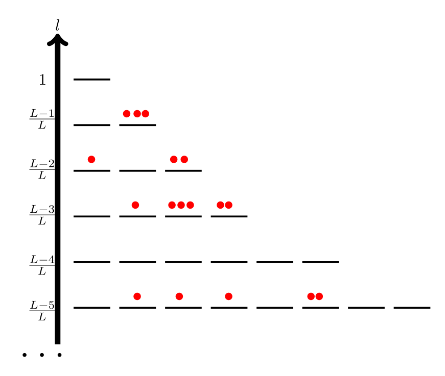
The non-conserving zero-range process with extensive rates of [9, 13] is formulated as a model of particles on a large fully-connected lattice. The vertices are called states. Each state can be occupied by any integer number of particles. Moreover, each state is equipped with a certain level of fitness (the higher the fitness is, the more particles are produced at the state per unit of time). The fitness levels are in [0,1], and they are regularly spaced by $L^{-1}$, where $L$ is a large integer. Moreover, the number $v_{k}$ of states at fitness level $k/L$ (for $k$ in $[1..L]$) is defined as:

$$v_{k}:=\mathrm{max}\left(\left[\frac{1}{L}q\left(\frac{k}{L}\right)V\right],1\right)=\frac{1}{L}q\left(\frac{k}{L}\right)V+\zeta_{k},\;\;\;\;\;\;\;(1\leq k\leq L),$$ (6)

where $V$ denotes a large integer, satisfying $V\gg L$, and the square brackets denote the integer part (which implies that the quantity $\zeta_{k}$ is in the interval $[-1,1]$). The symbol $q$ denotes a fixed probability density, defined on the continuum $[0,1]$, which is assumed to vanish at high fitness:

$$q(1)=0,\;\;\;\;\;\;q(l)\underset{l\to 1}{=}O\left((1-l)^{\alpha}\right),\;\;\;\;(\alpha>0).$$ (7)

It follows from Eq. (6) that there is exactly one state at the highest fitness level. A configuration of the system is sketched on Fig. 1 (showing the highest fitness levels).

Refer to caption
Figure 1: A schematic close-up of a configuration showing the occupation of the six highest fitness levels in the system. States are shown as horizontal bars, and particles as red dots. Numbers of states shown on the figure are for instance in our notations $v_{L}=1$, $v_{L-1}=2$, $v_{L-3}=4$, $v_{L-4}=6$. At fitness level $(L-3)/L$ there are $n_{(L-3)/L}=6$ particles. The occupation numbers of the corresponding $v_{L-3}$ states are $0,1,3,2$ in this configuration. There is no particle at maximum fitness in this configuration. The rate of appearance of a new particle at the maximum fitness level in this configuration is $1$ according to Eq. (14). There is no particle at fitness level $(L-4)/L$. A particle is added to this fitness level at rate $(L-4)/L$ according to Eq. (14), and sent to one of the $v_{L-4}$ states of fitness $(L-4)/L$ (drawn uniformly). This process is described equivalently in terms of states in Eq. (22): a particle is added to each of the $v_{L-4}=6$ states at rate $1/6$.

The fraction of the total number of states at fitness level $k/L$ follows from Eq. (6) as:

$$\frac{v_{k}}{\sum_{p=1}^{L}v_{p}}=\frac{\frac{1}{L}q\left(\frac{k}{L}\right)+\frac{\zeta_{k}}{V}}{\frac{1}{L}\sum_{p=1}^{L}q\left(\frac{p}{L}\right)+\frac{1}{V}\sum_{p=1}^{L}\zeta_{p}}.$$ (8)

In the large-$L$ limit we recognize a Riemann sum in the denominator

$$\frac{1}{L}\sum_{p=0}^{L}q\left(\frac{k}{L}\right)\simeq\int_{0}^{1}q(l)dl=1.$$ (9)

Moreover the assumption $V\gg L$ implies

$$\left|\frac{1}{V}\sum_{p=0}^{L}\zeta_{k}\right|\leq\frac{L}{V}=o(1).$$ (10)

In the limit of large $L$, with $V\gg L$, the probability density $q$ is therefore the density of states in the interval $[0,1]$ of possible fitness values:

$$\frac{v_{k}}{\sum_{p=0}^{L}v_{p}}\simeq\frac{1}{L}q\left(\frac{k}{L}\right).$$ (11)

The dynamics of the model was described in [9, 13] in terms of the occupation numbers of the fitness levels:

$$p_{l}(n,t):={\mathrm{Prob}}(n\;{\mathrm{particles}}\;{\mathrm{occupy}}\;{\mathrm{fitness}}\;{\mathrm{level}}\;l\;{\mathrm{at}}\;{\mathrm{time}}\;t).$$ (12)

The following three processes contribute to the dynamics:
1. Annihilation of particles. Particles die at fixed rate $\delta>0$. The total death rate at fitness level $l$ is therefore $\delta n$, where $n$ is the occupation number of this level. The annihilation process therefore induces the following term in the evolution111Time derivatives are denoted by $\frac{d}{dt}$ if time is the only variable taking values in a continuum. equation of $p_{l}$:

$$\left(\frac{dp_{l}(n,t)}{dt}\right)_{\mathrm{annihilation}}=-\delta np_{l}(n,t)\theta(n)+\delta(n+1)p_{l}(n+1,t),\;\;\;\;\;\;\;\;(n\in\mathbb{N}).$$ (13)

2. Creation of particles. Particles are created at a rate proportional to the fitness. The total rate of creation at fitness level $l$ is $l(n+1)$, if $n$ the occupation number of the level, hence the creation term

$$\left(\frac{dp_{l}(n,t)}{dt}\right)_{\mathrm{creation}}=lnp_{l}(n-1,t)\theta(n)-l(n+1)p_{l}(n,t),\;\;\;\;\;\;\;\;(n\in\mathbb{N}),$$ (14)

The creation rate is strictly positive for all values of $n$: if $n=0$, a particle is added to fitness level $l$ (this particle occupies a random state, drawn uniformly from the set of $v_{lL}$ states of fitness $l$). In the network interpretation of the model, this process corresponds to the acquisition of the first link by nodes in a network with a fixed set of nodes (and no existing links to any state of fitness $l$). This spontaneous-generation contribution ensures that the configuration with zero occupation number at all states is not a steady state.
3. Hopping to a uniformly chosen state. Particles hop at a constant rate $\beta>0$, performing a random walk on the network. This process induces

$$\begin{split}\left(\frac{dp_{l}(n,t)}{dt}\right)_{\mathrm{hopping}}=&\beta\rho(t)q(l)p_{l}(n-1,t)\theta(n)-\beta\rho(t)q(l)p_{l}(n,t)\\ &-\beta np_{l}(n,t)\theta(n)+\beta(n+1)p_{l}(n+1,t),\;\;\;\;\;\;\;\;(n\in\mathbb{N}).\\ \end{split}$$ (15)

where the density $\rho(t)$ is defined as the average occupation number of a fitness level,

$$\rho(t):=\int_{0}^{1}\overline{n_{l}}(t)dl,$$ (16)

and $\overline{n_{l}}(t)$ denotes the average occupation number of the fitness level $l$:

$$\overline{n_{l}}(t):=\sum_{m\geq 0}mp_{l}(m,t).$$ (17)

The occurrence of the density $\rho(t)$ in Eq. (15) is a consequence of the mean-field geometry. Indeed, the total number of particles hopping per unit of time is $\beta L\rho(t)$. The particles hop to uniformly-drawn states, hence the fitness level $l=k/L$ receives a fraction of the hopping particles equal to the fraction of the states in the system at fitness level. In the limit of large $L$, and $V\gg L$, this fraction equals the density of states at fitness level $l=k/L$, as explained in Eq. (11). We therefore obtain the rate at which particles hop to this fitness level:

$$\beta L\rho(t)\frac{v_{k}}{\sum_{p=0}^{L}v_{p}}\underset{\begin{subarray}{c}L\to\infty,\\ V\gg L\end{subarray}}{\simeq}\beta L\rho(t)\times\frac{1}{L}q\left(l\right)=\beta\rho(t)q\left(l\right),$$ (18)

which reproduces the coefficient in front of the first two terms in Eq. (15).

3 Zero-range process under local resetting

The evolution equation of the probability law $p_{l}$ of the occupation number of fitness level $l$, induced by the processes described in Eqs (13,14,15) was solved in [9, 13]. To subject the model to local resetting, we need to reformulate the three processes in terms of the occupation number of states. At a fixed fitness level $l=k/L$, the occupation numbers of the $v_{k}$ states are identically distributed. Let us label the states at this fitness level by an integer $s$ in $[1..v_{k}]$. and denote by $\pi_{l}$ the probability law of the number of particles in a state of fitness $l$:

$$\begin{split}\pi_{l}(n,t)={\mathrm{Prob}}(n\;{\mathrm{particles}}\;{\mathrm{occupy}}\;{\mathrm{state}}&\;s\;{\mathrm{of}}\;{\mathrm{fitness}}\;l\;{\mathrm{at}}\;{\mathrm{time}}\;t),\\ &\left(l=\frac{k}{L},\;1\leq k\leq L,\;1\leq s\leq v_{k}\right).\end{split}$$ (19)

In the large-$L$ limit, the model is in the mean-field geometry, and the probability of a list of occupation numbers $(n_{1},\dots,n_{v_{k}})$ of the $v_{k}$ states at fitness level $l=k/L$ is the product $\prod_{j=1}^{v_{k}}\pi_{l}(n_{j},t)$. This factorization property is a feature of the dynamics of urn models studied in [41, 2, 42, 43]. Given a total occupation number $M$ of the fitness level, the probability $p_{l}(M,t)$ is given as a sum over the partitions of the integer $M$ into $v_{k}$ nonnegative integers:

$$p_{l}(M,t)=\sum_{\begin{subarray}{c}\mathbf{n}=(n_{1},\dots,n_{v_{k}})\in\mathbb{N}^{v_{k}}\\ \sum_{j=1}^{v_{k}}n_{j}=M\end{subarray}}\prod_{j=1}^{v_{k}}\pi_{l}(n_{j},t),\;\;\;\;\;\;\;\;\;\left(M\in\mathbb{N},\;l=\frac{k}{L},\;1\leq k\leq L\right).$$ (20)

Let us define the creation, annihilation and hopping processes in terms of the quantities $(\pi_{k/L})_{1\leq i\leq v_{k}}$, so that the kinetic equations for the corresponding fitness level (displayed in Eqs (13,14,15)) are reproduced.

3.1 Annihilation process

The particles occupying a given state vanish at a rate $\delta>0$, hence the annihilation term

$$\begin{split}\left(\frac{d\pi_{l}(n,t)}{dt}\right)_{\mathrm{annihilation}}=-\delta n\pi_{l}(n,t)\theta(n)+\delta(n+1)\pi_{l}(n+1,t),\;\;\;\;\;\;\;\left(n\in\mathbb{N},l=\frac{k}{L},\;1\leq k\leq L\right).\end{split}$$ (21)

The above equation is intuitively equivalent to Eq. (13). The equivalence is derived explicitly in Appendix A using the relation between occupation numbers of states and fitness levels given in Eq. (20).

3.2 Creation process

The rates of creation of particles are biased by the fitness: let us define the rate of creation of particles at any state of fitness level $k/L$ to be $(k/L)\times\left(n+v_{k}^{-1}\right)$, where $n$ is the occupation number of the state. The constant term $(k/L)v_{k}^{-1}$ ensures that the process does not stop when all occupation numbers are zero (the factor of $v_{k}^{-1}$ intuitively corresponds to the $v_{k}$ choice of states in which to place a particle that is added at rate $k/L$ to the fitness level $k/L$ if it is empty). These rates induce the following creation term:

$$\begin{split}\left(\frac{d\pi_{l}(n,t)}{dt}\right)_{\mathrm{creation}}=l&\left(n-1+\frac{1}{v_{k}}\right)\pi_{l}(n-1,k/L,t)\theta(n)-l\left(n+\frac{1}{v_{k}}\right)\pi_{l}(n,k/L,t),\\ &\;\;\;\;\;\;\;\;\;\hskip 142.26378pt\left(n\in\mathbb{N},\;l=\frac{k}{L},\;1\leq k\leq L\right).\end{split}$$ (22)

It can easily be checked using Eq. (20) that the above equation induces the creation term displayed in Eq. (14) for the occupation number of the fitness level $l=k/L$. The corresponding calculations are reported in Appendix A.

3.3 Hopping process

The particles perform independent random walks on the fully-connected network of states. Each particle hops to a uniformly chosen state, with a fixed rate $\beta$. The fitness level $k/L$ receives per unit of time a fraction $\beta/Lq(k/L)$ of the total number of particles present in the system per unit of time, as explained in Eq. (18). These particles are shared equally between the $v_{k}$ states at this fitness level. The hopping process induces the following hopping term:

$$\begin{split}\left(\frac{d\pi_{l}(n,t)}{dt}\right)_{\mathrm{hopping}}=&\beta\frac{\rho(t)}{v_{k}}q(l)\pi_{l}(n-1,t)\theta(n)-\beta\frac{\rho(t)}{v_{k}}q(l)\pi_{l}(n,t)\\ &-\beta n\pi_{l}(n,t)\theta(n)+\beta(n+1)\pi_{l}(n+1,t),\\ &\;\;\;\;\;\;\;\;\;\hskip 142.26378pt\left(n\in\mathbb{N},\;l=\frac{k}{L},\;1\leq k\leq L\right).\end{split}$$ (23)

The above equation induces Eq. (15) thanks to Eq. (20), as explained in Appendix A.

3.4 Local-resetting process

In the global resetting prescription of [13], the occupation numbers of all the states in the system are set to zero simultaneously. These resetting events are Poisson-distributed mass-extinction events. The intensity of the corresponding Poisson process is the constant $r$ that appears in Eq. (5).

In the present model we take a local-resetting prescription, in which the occupation numbers of the states are independently reset to zero. The most general way to pick the intensities of the Poisson processes generating the resetting times (while ensuring that the occupation numbers at a fixed fitness level are identically distributed), is to make the rate of the Poisson process a function of the fitness. The $v_{k}$ Poisson processes attached to the states at fitness level $k/L$ are independent, and have the same intensity, which we will denote by $r(k/L)$. This local-resetting prescription induces the following terms in the evolution equation of the probability law of the occupation number at a state of given fitness $l$:

$$\begin{split}\left(\frac{d\pi_{l}(n,t)}{dt}\right)_{\mathrm{resetting}}=&-r(l)\pi_{l}(n,t)+r(l)\delta_{n,0},\\ &\;\;\;\;\;\;\;\;\;\hskip 85.35826pt\left(n\in\mathbb{N},\;l=\frac{k}{L},\;1\leq k\leq L\right).\end{split}$$ (24)

The function $r$ is an additional parameter of the model, a nonnegative function defined on $[0,1]$. The parameters of the non-conserving ZRP with extensive rates under local resetting are summarized in Table 1.

Symbol Values Particles Network Population
$l$ $l\in[0,1]$, approximated by $k/L$, with a large integer $L$ and $k$ in $[0..L]$ rate of production of particles (reproductive fitness) rate of acquisition of links (fitness of a node in a network) rate of cell division in a haploid population (reproductive fitness)
$v_{k}$ $v_{k}\in\mathbb{N}$ number of states at fitness level $k/L$ number of nodes at fitness level $k/L$ number of possible genomes with reproductive fitness $k/L$
$L$ large integer total number of distinct levels total number of distinct fitness levels total number of distinct fitness levels
$q(l)$ probability density on $[0,1]$, satisfying $q(1)=0$ and $q(l)\underset{l\to 1}{=}O((1-l)^{\alpha})$, with $\alpha>0$ density of states density of states mutant fitness
$\delta$ $\delta>0$ vanishing rate rate of disappearance of links death rate
$\beta$ $\beta>0$ hopping rate rewiring rate mutation rate
$r(l)$ nonnegative function of the fitness resetting rate of each state of fitness level $l$ to an empty configuration every node of fitness $l$ loses its links at rate $r(l)$ the population of every state of fitness $l$ goes extinct at rate $r(l)$
Table 1: Table of definitions and notations for the parameters of the model, with their interpretations in terms of particles, links in a network and haploid population dynamics.

3.5 Evolution equation of the occupation number of a state

Summing the terms described in Eqs (21,22,23,24) yields the evolution equation of the probability law of the occupation number of a state of given fitness $k/L$:

$$\begin{split}\frac{d\pi_{k/L}(n,t)}{dt}=\;&\theta(n)\left\{\left[\beta\frac{\rho(t)}{v_{k}}q\left(k/L\right)+\frac{k}{L}\left(n-1+\frac{1}{v_{k}}\right)\right]\pi_{k/L}(n-1,t)-(\beta+\delta)n\pi_{k/L}(n,t)\right\}\\ &+(\beta+\delta)(n+1)\pi_{k/L}(n+1,t)-\left[\beta\frac{\rho(t)}{v_{k}}q\left(k/L\right)+\frac{k}{L}\left(n+\frac{1}{v_{k}}\right)+r(k/L)\right]\pi_{k/L}(n,t)\\ &+r(k/L)\delta_{n,0},\;\;\;\;\;\;\;\;\vspace{2cm}(n\in{\mathbb{N}},1\leq k\leq L).\end{split}$$ (25)

Let us denote the average number of particles at fitness level $k/L$ by $\overline{n}_{k/L}(t)$. It also depends on the parameters hopping rate $\beta$, annihilation rate $\delta$, and on the density $q$, as well as the resetting rate $r(k/L)$, which for brevity is not reflected in the notation.
The average occupation number $\overline{n}_{k/L}(t)$ is the sum of the average occupation numbers at the $v_{k}$ states of fitness $k/L$:

$$\overline{n}_{k/L}(t)=\sum_{s=1}^{v_{k}}\sum_{m\geq 0}m\pi_{k/L}(m,t)=v_{k}\sum_{m\geq 0}m\pi_{k/L}(m,t).$$ (26)

Let us introduce the generating function of the probability of occupation numbers at a fixed state,

$$\chi(J,k/L,t):=\sum_{n\geq 0}\pi_{k/L}(n,t)J^{n}.$$ (27)

The average number of particles at a given fitness level $l=k/L$ (with $v_{k}=v_{lL}$ states) is therefore expressed in terms of the generating function as

$$\overline{n}_{l}(t)=v_{lL}\frac{\partial\chi(J,l,t)}{\partial J}|_{J=1}.$$ (28)

The expression of the density defined in Eq. (16) in terms of the generating function follows as

$$\rho(t)=\int_{0}^{1}dlv_{lL}\frac{\partial\chi(J,l,t)}{\partial J}|_{J=1}.$$ (29)

To obtain the analogue of Eq. (5) in the model with local resetting, we are therefore instructed to work out and solve the evolution equation of the generating function $\chi$.

4 Generating function

4.1 Evolution equation of the generating function

Using the identity

$$\sum_{n\geq 1}n\pi_{l}(n,t)J^{n}=J\frac{\partial\chi}{\partial J}(J,l,t),$$ (30)

we obtain the evolution equation of the generating function $\chi$ (defined in Eq. (27)) as a PDE of order one in $J$ and in time. At a fitness level $l=k/L$, there are $v_{k}=v_{lL}$ states, and the generating function of the probability law of the occupation number at each of these states satisfies

$$\begin{split}\frac{\partial\chi(J,l,t)}{\partial t}=r(l)+&\left[(1-J)\left(-\frac{l}{v_{lL}}-\beta\frac{\rho(t)}{v_{lL}}q(l)\right)-r(l)\right]\chi(J,l,t)\\ &+(1-J)\left(\beta+\delta-lJ\right)\frac{\partial\chi(J,l,t)}{\partial J}.\end{split}$$ (31)

This evolution equation is nonlinear, because the density $\rho$ is expressed in terms of the generating function (see Eq. (29)).

As in [13], we can apply the method of characteristics to solve the PDE, provided the density $\rho(t)$ is treated as a parameter. The solution is derived in Appendix B and reads

$$\begin{split}\chi(J,l,t)=&\chi\left(1-\frac{(l-1-\zeta)(1-J)}{l(1-J)-\left(l(1-J)+(1+\zeta-l)\right)e^{(1+\zeta-l)t}},l,0\right)\\ &\times\exp\left(-r(l)t-\frac{(l-1-\zeta)(1-J)}{v_{lL}}\int_{0}^{t}ds\frac{l+\beta\rho(s)q(l)}{l(1-J)-(1+\zeta-lJ)e^{(1+\zeta-l)(t-s)}}\right)\\ &+r(l)\int_{0}^{t}du\exp\left(-r(l)u-\frac{(l-1-\zeta)(1-J)}{v_{lL}}\int_{0}^{u}dz\frac{l+\beta\rho(t-z)q(l)}{l(1-J)-(1+\zeta-lJ)e^{(1+\zeta-l)z}}\right).\end{split}$$ (32)

where the notation $\zeta$ has been introduced to denote the combination of hopping and annihilation rates:

$$\zeta:=\beta+\delta-1.$$ (33)

In these notations (introduced in [9]), the annihilation rate is described by the parameter $\zeta$, and the parameter $\delta$ does not appear. At this point we have to impose consistency with the definition of the density in Eq. (29).

4.2 Closure condition on the density

The average occupation number of the fitness level $l$ at time $t$, expressed Eq. (28), is readily calculated by Taylor expansion of the generating function:

$$\begin{split}\chi(J,l,t)=1+(J-1)\frac{\partial\chi}{\partial J}(J,l,t)|_{J=1}+o(J-1).\end{split}$$ (34)

The calculation is shown in Appendix C and yields the average occupation number at fitness level $l$ as

$$\begin{split}\overline{n_{l}}(t)=&\overline{n_{l}}(0)e^{-(1+\zeta+r(l)-l)t}\\ &+\frac{l}{1+\zeta+r(l)-l}\left(1-e^{-(1+\zeta+r(l)-l)t}\right)+\beta q(l)\int_{0}^{t}\rho(t-s)e^{-(1+\zeta+r(l)-l)s}ds.\end{split}$$ (35)

The number $v_{lL}$ of states at fitness level $l$ does not appear explicitly in this expression, because each of the $v_{lL}$ states at this fitness level contributes the same average occupation number.

Let us denote the Laplace transform of a function $f$ of time by $\widetilde{f}$:

$$\widetilde{f}(s):=\int_{0}^{\infty}dte^{-st}f(t).$$ (36)

The Laplace transform maps convolution products to ordinary products. The occupation number of fitness level $l$ is therefore obtained from Eq. (35) in Laplace space as

$$\begin{split}\widetilde{\overline{n_{l}}}(s)=&\frac{\overline{n_{l}}(0)}{1+\zeta+r(l)-l+s}\\ &+\frac{l}{1+\zeta+r(l)-l}\left(\frac{1}{s}-\frac{1}{1+\zeta+r(l)-l+s}\right)+\widetilde{\rho}(s)\frac{\beta q(l)}{1+\zeta+r(l)-l+s}.\end{split}$$ (37)

Integrating w.r.t. the fitness $l$ and using the definition in Eq. (16) yields the closure condition on the density in Laplace space

$$\begin{split}\widetilde{\rho}(s)=&\int_{0}^{1}dl\frac{\overline{n_{l}}(0)}{1+\zeta+r(l)-l+s}\\ &+\int_{0}^{1}dl\frac{l}{s(1+\zeta+r(l)-l+s)}+\beta\widetilde{\rho}(s)\int_{0}^{1}dl\frac{q(l)}{1+\zeta+r(l)-l+s}.\end{split}$$ (38)

We therefore obtain the Laplace transform of the density as

$$\widetilde{\rho}(s)=\frac{1}{s}\frac{s\int_{0}^{1}dl\frac{\overline{n_{l}}(0)}{1+\zeta+r(l)-l+s}+\int_{0}^{1}dl\frac{l}{1+\zeta+r(l)-l+s}}{1-\beta\int_{0}^{1}dl\frac{q(l)}{1+\zeta+r(l)-l+s}}.$$ (39)

This expression, which can be substituted into Eq. (37), yields the average occupation of the each fitness level in Laplace space. In particular, it can be used to obtain the steady-state values of these occupation numbers.

5 Steady state of the system

5.1 Distribution of fitness in the steady state

If the system reaches a steady state, the density reaches a positive value $\rho(\infty)$ which is given by the final-value theorem:

$$\rho(\infty)=\underset{s\to 0}{\lim}s\widetilde{\rho}(s).$$ (40)

The steady-state value of the density is expressed in terms of the death rate, hopping rate, resetting rate and density of states as

$$\rho(\infty)=\frac{1}{1-\frac{\beta}{\beta_{c}}}\int_{0}^{1}dl\frac{l}{1+\zeta+r(l)-l},$$ (41)

which is positive provided $\beta<\beta_{c}$, where the quantity $\beta_{c}$ is the critical value of the mutation rate defined as

$$\beta_{c}=\left(\int_{0}^{1}dl\frac{q(l)}{1+\zeta+r(l)-l}\right)^{-1}.$$ (42)

As the function $r$ is nonnegative, all the integrals in Eqs (41,42) converge if $\zeta>0$. Moreover, the critical value $\beta_{c}$ is greater than the upper bound on the hopping rate that appears in the model without resetting (given in Eq. (3)):

$$\left(\int_{0}^{1}dl\frac{q(l)}{1+\zeta-l}\right)^{-1}\leq\beta_{c}.$$ (43)

Hence, if the parameters lead to a steady state in the model without resetting (which is the case if $\beta<\left(\int_{0}^{1}dl\frac{q(l)}{1+\zeta-l}\right)^{-1}$), the condition $\beta<\beta_{c}$ is satisfied and the system under local resetting reaches a steady state for any choice of the function $r$.

Applying the final-value theorem to Eq. (37) yields

$$\begin{split}\overline{n_{l}}(\infty)=&\underset{s\to 0}{\lim}s\widetilde{\overline{n_{l}}}(s)\\ =&\frac{l}{1+\zeta+r(l)-l}+\rho(\infty)\frac{\beta q(l)}{1+\zeta+r(l)-l}.\end{split}$$ (44)

The steady state of the system does not depend on the initial conditions because $\overline{n_{l}}(0)$ does not appear in Eq. (41,44). The expression of the steady-state average occupation number, average density and critical hopping rate are formally identical to the expression obtained in [13] in the model subjected to global resetting, and reported in Eq. (5).

5.2 Condensation at high fitness in the limit of high density

In the ordinary model (without resetting, see Eq. (4)), the density $\rho(\infty)$ goes to infinity and an atom appears at high fitness in the limit where the sum of hopping rate and annihilation rate decreases to the maximum value of the fitness (in our notations this limit is $\zeta\to 0^{+}$), at a fixed of the hopping rate satisfying

$$\beta<\left(\int_{0}^{1}\frac{q(l)dl}{1-l}\right)^{-1}.$$ (45)

The behavior of the first term in Eq. (44) in this limit depends on the local behavior of the resetting rate $r(l)$ close to $l=1$. If the resetting rate vanishes at maximum fitness, this term goes to infinity when $\zeta$ goes to 00. To identify a limit of high density in the system with local resetting, we must let $r(l)$ go to zero when $l$ goes to the maximum fitness value $1$. Let us assume that the resetting rate vanishes at maximum fitness with a power-law behavior. There exist two positive constants $C$ and $\nu$ such that

$$r(l)\underset{l\to 1}{\sim}C(1-l)^{\nu}.$$ (46)

Let us distinguish three cases, depending on whether the resetting rate vanishes linearly ($\nu=1$), sublinearly ($\nu<1$) or superlinearly ($\nu>1$). In all cases, the integral defining the critical value of the hopping rate $\beta$ defined in Eq. (42) has a finite limit when $\zeta$ goes to zero, because of the assumption $q(l)\underset{l\to 1}{=}O((1-l)^{\alpha})$ made in Eq. (7):

$$\underset{\zeta\to 0^{+}}{\lim}\beta_{c}^{-1}=\int_{0}^{1}dl\frac{q(l)}{1+r(l)-l}.$$ (47)

Indeed the integrand vanishes at maximum fitness as $(1-l)^{\alpha-1}$ if $\nu\geq 1$, and as $(1-l)^{\alpha-\nu}\ll(1-l)^{\alpha-1}$ if $\nu<1$. Moreover, a fixed hopping rate $\beta<\left(\int_{0}^{1}dl\frac{q(l)}{1+r(l)-l}\right)^{-1}$ satisfies the condition $\beta<\left(\int_{0}^{1}dl\frac{q(l)}{1+\zeta+r(l)-l}\right)^{-1}$ for $\zeta>0$, which ensures a steady state is reached. Hence we can study the limit $\zeta\to 0^{+}$ for any such value of $\beta$ using the results obtained in Eqs (41,44).

5.2.1 Sublinearly vanishing resetting rate at high fitness ($\nu<1$)

Consider the case $\nu<1$. If $\zeta=0$, the denominators in the expression of the average occupation numbers (Eq. (44)) are equivalent to the resetting rate when the fitness is close to its maximum value:

$$1-l+r(l)\underset{l\to 1}{\sim}C(1-l)^{\nu}.$$ (48)

Hence all the integrals in the expression of the average occupation numbers are finite in the small-$\zeta$ limit:

$$\begin{split}\underset{\zeta\to 0^{+}}{\lim}\overline{n_{l}}(\infty)=&\frac{l}{1+r(l)-l}+\rho(\infty)\frac{\beta q(l)}{1+r(l)-l},\\ \underset{\zeta\to 0^{+}}{\lim}\rho(\infty)=&\int_{0}^{1}\frac{ldl}{1-l+r(l)}+\int_{0}^{1}\frac{\beta q(l)dl}{1+r(l)-l}.\end{split}$$ (49)

The density and all the occupation number have a finite limit when $\zeta$ goes to $0^{+}$, as in the model with global resetting.

5.2.2 Linearly vanishing resetting rate at high fitness

The resetting rate has the following behavior at high fitness:

$$r(l)\underset{l\to 1}{\sim}C(1-l).$$ (50)

The quantities $1-l$ and $r(l)$ are of the same order close to maximum fitness. The change of variables from the fitness $l$ to $h$ defined by $l=1-\zeta h$ yields

$$\int_{0}^{1}dl\frac{l}{1+\zeta+r(l)-l}=\zeta\int_{0}^{\frac{1}{\zeta}}\frac{1-\zeta h}{\zeta h+r(1-\zeta h)+\zeta}.$$ (51)

Maximum fitness corresponds to $h=0$. Taylor expansion close to this value yields

$$\begin{split}\zeta h+r(1-\zeta h)+\zeta=&\zeta\left(1+(C+1)h+o(1)\right),\\ \int_{0}^{1}dl\frac{l}{1+\zeta+r(l)-l}=&\int_{0}^{\frac{1}{\zeta}}\frac{(1+o(1))dh}{1+(C+1)h}.\end{split}$$ (52)

On the other hand,

$$\begin{split}\int_{0}^{\frac{1}{\zeta}}\frac{(1+o(1))dh}{1+(C+1)h}&=\frac{1}{C+1}\int_{0}^{\frac{1}{(C+1)\zeta}}\frac{dz}{1+z}\\ &=\frac{1}{C+1}\log\left(1+\frac{1}{(C+1)\zeta}\right)=\frac{1}{C+1}\left[\log(\zeta^{-1})+\log\left(\zeta+\frac{1}{C+1}\right)\right]\\ &\underset{\zeta\to 0^{+}}{\sim}-\frac{1}{C+1}\log(\zeta),\end{split}$$ (53)

hence the equivalent

$$\begin{split}\int_{0}^{1}dl\frac{l}{1+\zeta+r(l)-l}\underset{\zeta\to 0^{+}}{\sim}-\frac{1}{C+1}\log(\zeta).\end{split}$$ (54)

The density diverges logarithmically when $\zeta$ goes to zero, with a prefactor depending on the local form of the resetting rate at maximum fitness:

$$\rho(\infty)\underset{\zeta\to 0^{+}}{\sim}\frac{-\log\zeta}{(C+1)\left(1-\beta\int_{0}^{1}\frac{q(l)dl}{1-l+r(l)}\right)}.$$ (55)

Consider a smooth test function $\phi$ defined on the interval $[0,1]$. Let us study the small-$\zeta$ limit of the integral of $\phi$ against the average occupation number of the steady state:

$$\begin{split}\int_{0}^{1}\frac{l\phi(l)dl}{1+\zeta+r(l)-l}=&\zeta\int_{0}^{\frac{1}{\zeta}}\frac{(1-\zeta h)\phi(1-\zeta h)dh}{\zeta h+C\zeta h+\zeta}=\phi(1)\int_{0}^{\frac{1}{\zeta}}\frac{dh}{1+(C+1)h}\left(1+o(1)\right)\\ &\underset{\zeta\to 0^{+}}{\sim}-\frac{\log(\zeta)}{C+1}\phi(1).\\ \end{split}$$ (56)
$$\begin{split}\int_{0}^{1}dl\phi(l)\overline{n_{l}}(\infty)&\underset{\zeta\to 0^{+}}{\sim}-\frac{\log(\zeta)}{C+1}\phi(1)-\beta\frac{\log(\zeta)}{(C+1)\left(1-\beta\int_{0}^{1}\frac{q(l)dl}{1-l+r(l)}\right)}\int_{0}^{1}\frac{q(l)\phi(l)dl}{1+r(l)-l}.\end{split}$$ (57)

Hence, dividing both sides by $\rho(\infty)$ and using the equivalent of the density worked obtained in Eq. (55) yields

$$\begin{split}\frac{1}{\rho(\infty)}\int_{0}^{1}dl\phi(l)\overline{n_{l}}(\infty)\underset{\zeta\to 0^{+}}{\sim}\left(1-\beta\int_{0}^{1}\frac{q(l)dl}{1-l+r(l)}\right)\phi(1)+\beta\int_{0}^{1}\frac{q(l)\phi(l)dl}{1+r(l)-l}.\end{split}$$ (58)

Liberating the test function yields the following limit for the density of occupation numbers (for a fixed hopping rate $\beta<\left(\int_{0}^{1}\frac{q(l)dl}{1+r(l)-l}\right)^{-1}$):

$$\frac{1}{\rho(\infty)}\overline{n_{l}}(\infty)\underset{\delta\to(1-\beta)^{+}}{\sim}\left(1-\beta\int_{0}^{1}\frac{q(l)dl}{1-l+r(l)}\right)\delta_{1}+\beta\frac{q(l)}{1+r(l)-l}.$$ (59)

There is a an atom at maximum fitness in the limit of high density.

5.2.3 Superlinearly vanishing resetting rate at high fitness ($\nu>1$)

In this case the resetting rate is subdominant at high fitness compared to the term $1-l$. For small $\zeta$, let us define again the variable $h$ by $l=1-\zeta h$. Eq. (51) still holds. In the limit of small $\zeta$, the expansion $r(1-\zeta h)=C(\zeta h)^{\nu}+o(\zeta^{\nu})$ induces (at fixed $h$)

$$\begin{split}\zeta h+r(1-\zeta h)+\zeta=&\zeta\left(1+h+Ch^{\nu}\zeta^{\nu-1}+o(\zeta^{\nu-1})\right)=\zeta\left(1+h+o(1)\right),\\ \int_{0}^{1}dl\frac{l}{1+\zeta+r(l)-l}=&\int_{0}^{\frac{1}{\zeta}}\frac{(1+o(1))dh}{1+h}\underset{\zeta\to 0^{+}}{\sim}-\log(\zeta).\end{split}$$ (60)

On the other hand, the integral in the definition of the critical mutation rate has a finite limit when $\zeta$ goes to zero because the density $q$ goes to zero at high fitness, hence

$$\rho(\infty)\underset{\zeta\to 0^{+}}{\sim}\frac{-\log\zeta}{1-\beta\int_{0}^{1}\frac{q(l)dl}{1-l+r(l)}}.$$ (61)

Given a smooth test function $\phi$ defined on the interval $[0,1]$, we obtain:

$$\begin{split}\int_{0}^{1}dl\phi(l)\overline{n_{l}}(\infty)=&\int_{0}^{1}\frac{l\phi(l)dl}{1+\zeta+r(l)-l}+\beta\rho(\infty)\int_{0}^{1}\frac{q(l)\phi(l)dl}{1+\zeta+r(l)-l}\\ \end{split}$$ (62)

Let us apply the same change of variables as above to obtain an equivalent of the first term:

$$\begin{split}\int_{0}^{1}\frac{l\phi(l)dl}{1+\zeta+r(l)-l}=&\zeta\int_{0}^{\frac{1}{\zeta}}\frac{(1-\zeta h)\phi(1-\zeta h)dh}{\zeta h+r(1-\zeta h)+\zeta}=\phi(1)\int_{0}^{\frac{1}{\zeta}}\frac{dh}{1+h}\left(1+o(1)\right)\\ &\underset{\zeta\to 0^{+}}{\sim}-\log(\zeta)\phi(1).\\ \end{split}$$ (63)

Using the equivalent of the average density obtained in Eq. (61), we notice that both terms on the r.h.s. of Eq. (62) are of order $-\log\zeta$:

$$\begin{split}\int_{0}^{1}dl\phi(l)\overline{n_{l}}(\infty)&\underset{\zeta\to 0^{+}}{\sim}-\log(\zeta)\phi(1)-\beta\frac{\log(\zeta)}{1-\beta\int_{0}^{1}\frac{q(l)dl}{1-l+r(l)}}\int_{0}^{1}\frac{q(l)\phi(l)dl}{1+r(l)-l}.\end{split}$$ (64)

Hence

$$\begin{split}\frac{1}{\rho(\infty)}\int_{0}^{1}dl\phi(l)\overline{n_{l}}(\infty)\underset{\zeta\to 0^{+}}{\sim}\left(1-\beta\int_{0}^{1}\frac{q(l)dl}{1-l+r(l)}\right)\phi(1)+\beta\int_{0}^{1}\frac{q(l)\phi(l)dl}{1+r(l)-l}.\end{split}$$ (65)

We read off the distribution of fitness in the steady state in the limit of high density (for a fixed hopping rate $\beta<\left(\int_{0}^{1}\frac{q(l)dl}{1+r(l)-l}\right)^{-1}$):

$$\frac{1}{\rho(\infty)}\overline{n_{l}}(\infty)\underset{\delta\to(1-\beta)^{+}}{\sim}\left(1-\beta\int_{0}^{1}\frac{q(l)dl}{1-l+r(l)}\right)\delta_{1}+\beta\frac{q(l)}{1+r(l)-l}.$$ (66)

In the limit of high density, the distribution of fitness develops an atom at maximum fitness. The mass of this atom is expressed by adding the resetting rate to the combination of hopping and annihilation rates in the expression of the mass of the condensate in the ordinary model, reported in Eq. (4).

6 Discussion

In this work we have worked out in closed form the steady state of a ZRP with extensive rates on a fully-connected lattice, with states subjected to local resetting. The mean-field geometry allowed to formulate the dynamics in terms of the probability law of the occupation numbers of the states. In the local-resetting prescription, the occupation number of any state in the system is set to zero at Poisson-distributed times (the corresponding Poisson process has a rate $r(l)$ that depends only on the fitness level of the state). In the network interpretation of the model, all links pointing to a given vertex disappear at resetting events. In the population-dynamics interpretation, all bacteria present at a given state die at resetting events.

The mean occupation numbers of the fitness levels take the same form as the result obtained in [13], where the system was subjected to global resetting. The only difference is the dependence of the resetting rate on the fitness level. This formal coincidence emerges in the steady state, but the solution of the evolution equation involves the resetting rate $r(l)$ at every fitness level $l$, whereas the derivation of [13] applied a renewal argument to the solution of the evolution equation in the ordinary model. The dependence of the occupation numbers on the resetting rate allows for a condensate to form in the limit where the combined hopping and death rate decrease to the maximum value of the fitness. The formation of an atom depends only on the local behavior of the resetting rate at high fitness: a condensate can form in the limit of high density if the resetting rate $r(l)$ goes to zero at least as fast as $(1-l)$ when the fitness $l$ goes to its maximal value $1$. This result suggests that local resetting may have deep consequences on the phases of an interacting particle system, particularly when the resetting rate depends on the state of the particles. To test this idea in a model with a phase transition, one could for example consider a model of binary aggregation with multiplicative kernel, for which a gelation transition occurs at finite time [44, 45] (see Chapter 5 of [46] for a review), and reset polymers to monomers, at a rate depending on their size.

More realistic versions of the Kingman model include randomness in the mutation rate [47, 48]. Alternatively, we could generalize the present model by introducing independent identically-distributed sources of noise to the local resetting rate. The case of unbounded fitness was studied in the limit of large populations in [49]. It would be interesting to see whether resetting could interfere with the wave-form of the solution moving towards higher fitnesses. Local resetting could perhaps be realized experimentally in a modified Lenski experiment [50, 51] (in the ongoing Lenski experiment the fitness of a growing bacterial population is studied through regular sampling after exposure to a glucose-based growth medium). Fluctuations in the availability of the nutrient could result in the selective annihilation of bacteria with lower fitness.

Appendix A Evolution equation for the occupation number of a fitness level

Consider a fixed fitness level

$$l:=\frac{k}{L},\;\;\;\;\;\;\;\;\;\;\;\hskip 28.45274pt(k\in[1..L]).$$ (67)

The probability law $\pi_{l}$ of the occupation numbers of each the $v_{k}$ states at this fitness level is related to the probability law $p_{l}$ of the occupation number of the entire fitness level $l$ by Eq. (20). The evolution equation of $p_{l}$ is therefore induced by the evolution equation of $\pi_{l}$ as follows:

$$\frac{dp_{l}(M,t)}{dt}=\sum_{\begin{subarray}{c}\mathbf{n}=(n_{1},\dots,n_{v_{k}})\in\mathbb{N}^{v_{k}}\\ \sum_{j=1}^{v_{k}}n_{j}=M\end{subarray}}\sum_{u=1}^{v_{k}}\frac{d\pi_{l}(n_{u},t)}{dt}\prod_{\begin{subarray}{c}1\leq j\leq v_{k}\\ j\neq u\end{subarray}}\pi_{l}(n_{j},t).$$ (68)

Consider the contribution to the r.h.s. of the term proposed in Eq. (22) to model the creation process:

$$\begin{split}&\sum_{\begin{subarray}{c}\mathbf{n}=(n_{1},\dots,n_{v_{k}})\in\mathbb{N}^{v_{k}}\\ \sum_{j=1}^{v_{k}}n_{j}=M\end{subarray}}\sum_{u=1}^{v_{k}}\left(\frac{d\pi_{l}(n_{u},t)}{dt}\right)_{\mathrm{creation}}\prod_{\begin{subarray}{c}1\leq j\leq v_{k}\\ j\neq u\end{subarray}}\pi_{l}(n_{j},t)\\ =&\sum_{\begin{subarray}{c}\mathbf{n}=(n_{1},\dots,n_{v_{k}})\in\mathbb{N}^{v_{k}}\\ \sum_{j=1}^{v_{k}}n_{j}=M\end{subarray}}\sum_{u=1}^{v_{k}}\left[l\left(n_{u}-1+\frac{1}{v_{k}}\right)\pi_{l}(n_{u}-1,l,t)\theta(n_{u})-l\left(n_{u}+\frac{1}{v_{k}}\right)\pi_{l}(n_{u},l,t)\right]\prod_{\begin{subarray}{c}1\leq j\leq v_{k}\\ j\neq u\end{subarray}}\pi_{l}(n_{j},t).\end{split}$$ (69)

Let us express the following two terms in terms of the probability law $p_{l}$ of the occupation number of the fitness level $l$:

$$\begin{split}\sum_{\begin{subarray}{c}\mathbf{n}=(n_{1},\dots,n_{v_{k}})\in\mathbb{N}^{v_{k}}\\ \sum_{j=1}^{v_{k}}n_{j}=M\end{subarray}}\sum_{u=1}^{v_{k}}\Xi_{k}n_{u}\pi_{k}(n_{u},t)\prod_{\begin{subarray}{c}1\leq j\leq v_{k}\\ j\neq u\end{subarray}}\pi_{k}(n_{j},t)=&\sum_{\begin{subarray}{c}\mathbf{n}=(n_{1},\dots,n_{v_{k}})\in\mathbb{N}^{v_{k}}\\ \sum_{j=1}^{v_{k}}n_{j}=M\end{subarray}}\sum_{u=1}^{v_{k}}n_{u}\prod_{1\leq j\leq v_{k}}\pi_{k}(n_{j},t)\\ =&\Xi_{k}\sum_{\begin{subarray}{c}\mathbf{n}=(n_{1},\dots,n_{v_{k}})\in\mathbb{N}^{v_{k}}\\ \sum_{j=1}^{v_{k}}n_{j}=M\end{subarray}}\left(\prod_{1\leq j\leq v_{k}}\pi_{k}(n_{j},t)\right)\sum_{u=1}^{v_{k}}n_{u}\\ =&M\Xi_{k}\sum_{\begin{subarray}{c}\mathbf{n}=(n_{1},\dots,n_{v_{k}})\in\mathbb{N}^{v_{k}}\\ \sum_{j=1}^{v_{k}}n_{j}=M\end{subarray}}\left(\prod_{1\leq j\leq v_{k}}\pi_{k}(n_{j},t)\right)\\ =&M\Xi_{k}p_{l}(M,t),\end{split}$$ (70)
$$\begin{split}\sum_{\begin{subarray}{c}\mathbf{n}=(n_{1},\dots,n_{v_{k}})\in\mathbb{N}^{v_{k}}\\ \sum_{j=1}^{v_{k}}n_{j}=M\end{subarray}}\sum_{u=1}^{v_{k}}\Xi_{k}\pi_{k}(n_{u},t)\prod_{\begin{subarray}{c}1\leq j\leq v_{k}\\ j\neq u\end{subarray}}\pi_{k}(n_{j},t)=&\Xi_{k}\sum_{\begin{subarray}{c}\mathbf{n},\sum_{j=1}^{v_{k}}n_{j}=m\end{subarray}}\sum_{u=1}^{v_{k}}\prod_{1\leq j\leq v_{k}}\pi_{k}(n_{j},t)\\ =&\Xi_{k}p_{l}(m,t),\end{split}$$ (71)

where $\Xi_{k}$ is a quantity that may depend on the integer $k$ and on time (like $v_{k}^{-1}$, $l$, $\delta$ or $\beta\rho(t)$) but not on any of the integers $(n_{1},\dots,n_{v_{k}})$.

Applying the two identities derived in Eqs (70,71), with $l$ and $l/v_{k}$ substituted to $\Xi_{k}$, the r.h.s. of Eq. (69) becomes

$$\begin{split}\sum_{\begin{subarray}{c}\mathbf{n}=(n_{1},\dots,n_{v_{k}})\in\mathbb{N}^{v_{k}}\\ \sum_{j=1}^{v_{k}}n_{j}=M\end{subarray}}\left(\frac{d\pi_{l}(n_{u},t)}{dt}\right)_{\mathrm{creation}}&\prod_{\begin{subarray}{c}1\leq j\leq v_{k}\\ j\neq u\end{subarray}}\pi_{l}(n_{j},t)\\ &=l\left(M-1+\frac{1}{v_{k}}\right)\theta(n)p_{l}(M-1,t)-l\left(M+\frac{1}{v_{k}}\right)p_{l}(M,t)\\ &=\left(\frac{dp_{l}(M,t)}{dt}\right)_{\mathrm{creation}},\end{split}$$ (72)

which proves that the creation term defined for the fitness level in Eq. (14) is induced by the creation terms for the occupation number of the states as defined in Eq. (22). Similarly, substituting the parameters $\delta$, $\beta$ and $\beta\rho(t)v_{k}^{-1}$ to the quantity $\Xi_{k}$, we obtain

$$\begin{split}\sum_{\begin{subarray}{c}\mathbf{n}=(n_{1},\dots,n_{v_{k}})\in\mathbb{N}^{v_{k}}\\ \sum_{j=1}^{v_{k}}n_{j}=M\end{subarray}}\left(\frac{d\pi_{l}(n_{u},t)}{dt}\right)_{\mathrm{annihilation}}\prod_{\begin{subarray}{c}1\leq j\leq v_{k}\\ j\neq u\end{subarray}}\pi_{l}(n_{j},t)&=\left(\frac{dp_{l}(M,t)}{dt}\right)_{\mathrm{annihilation}},\\ \sum_{\begin{subarray}{c}\mathbf{n}=(n_{1},\dots,n_{v_{k}})\in\mathbb{N}^{v_{k}}\\ \sum_{j=1}^{v_{k}}n_{j}=M\end{subarray}}\left(\frac{d\pi_{l}(n_{u},t)}{dt}\right)_{\mathrm{hopping}}\prod_{\begin{subarray}{c}1\leq j\leq v_{k}\\ j\neq u\end{subarray}}\pi_{l}(n_{j},t)&=\left(\frac{dp_{l}(M,t)}{dt}\right)_{\mathrm{hopping}}.\end{split}$$ (73)

The expressions proposed in Eqs (21,23) are therefore consistent with the dynamics of the fitness level described by Eqs (13,15).

Appendix B Characteristic curves for the generating function

Let us look for a change of variables from $(J,l,t)$ to some new variables $(v,l,t)$, so that the generating function expressed in terms of the new variables satisfies an ordinary differential equation. Let us denote by $\hat{\chi}$ the generating function expressed in terms of the new variables:

$$\hat{\chi}(v,l,t):=\chi(J(v,l,t),l,t).$$ (74)

Taking the derivative of Eq. (74) w.r.t. time we obtain:

$$\frac{\partial\hat{\chi}(v,l,t)}{\partial t}=\frac{\partial\chi(J(v,l,t),l,t)}{\partial J}\frac{\partial J(v,l,t)}{\partial t}+\frac{\partial\chi(J(v,l,t),l,t)}{\partial t}.$$ (75)

Inspecting Eq. (31), we impose the following condition so that the coefficient of the derivative $\partial\chi/\partial J$ equals zero:

$$\frac{\partial J}{\partial t}=(J-1)\left(\beta+\delta-lJ\right).$$ (76)

The average density $\rho$ is a function of time only, and the probability density $q$ is a function of the fitness only. Their expression does not change when we change variables from $(J,l,t)$ to $(v,l,t)$. We therefore rewrite Eq. (31) in the variables $(v,l,t)$ as

$$\frac{\partial\hat{\chi}(v,l,t)}{\partial t}=r(l)-r(l)\hat{\chi}(v,l,t)+\left(1-J(v,l,t)\right)\left(-\frac{l}{v_{k}}-\beta\frac{\rho(t)}{v_{k}}q(l)\right)\hat{\chi}(v,l,t),$$ (77)

where $l=k/L$, and $v_{k}$ is the number of states at fitness level $l$. The condition obtained in Eq. (76) is a differential equation, which was solved as follows in [13]. The inverse of the r.h.s. is a rational function of the parameter $J$, which is easily decomposed into simple elements. Assuming that the sum of the creation and annihilation rates is greater than the maximum fitness, we write

$$\beta+\delta=1+\zeta,$$ (78)

for some $\zeta>0$. The two poles of the rational fraction in Eq. (79) are therefore distinct, and

$$\frac{1}{(J-1)(\beta+\delta-lJ)}=\frac{1}{\beta+\delta-l}\left(\frac{1}{J-1}-\frac{l}{lJ-\beta-\delta}\right).$$ (79)

The quantity $lJ-1-\zeta$ is negative if $J$ is in the interval $[0,1]$. Restricting $J$ to this interval, we rewrite Eq. (76) as follows:

$$\frac{1}{1+\zeta-l}\left(\frac{\partial\log(1-J)}{\partial t}-\frac{\partial\log(1+\zeta-lJ)}{\partial t}\right)=1,\;\;\;\;(0\leq J\leq 1),$$ (80)

which reads as an equality between time derivatives:

$$\frac{\partial}{\partial t}\left(\log\left(\frac{1+\zeta-lJ(v,l,t)}{1-J(v,l,t)}\right)\right)=\frac{\partial}{\partial t}\left((l-1-\zeta)t\right).$$ (81)

Integrating w.r.t. time between 00 and a fixed positive time, denoting by $v$ the integration constant on the r.h.s. yields

$$\int_{0}^{T}dt\frac{\partial}{\partial t}\left(\log\left(\frac{1+\zeta-lJ(v,l,t)}{1-J(v,l,t)}\right)\right)=\int_{0}^{T}dt\frac{\partial}{\partial t}\left((l-1-\zeta)t\right).$$ (82)
$$\log\left(\frac{1+\zeta-lJ(v,l,t)}{1-J(v,l,t)}\right)=v+(l-1-\zeta)t.$$ (83)

The change of variables from $(J,l,t)$ to $(v,l,t)$ is therefore defined by the relation:

$$\frac{1+\zeta-lJ(v,l,t)}{1-J(v,l,t)}=e^{v}e^{(l-1-\zeta)t}.$$ (84)

We can express the factor of $(1-J)$ needed in Eq. 77 in the variables $(v,l,t)$ as:

$$1-J(v,l,t)=\frac{l-1-\zeta}{l-e^{v}e^{(l-1-\zeta)t}}.$$ (85)

Substituting into Eq. (77) yields an explicit form in terms of the variables $(v,l=k/L,t)$ for the time-evolution of the generating function:

$$\frac{\partial\hat{\chi}(v,l,t)}{\partial t}=r(l)-r(l)\hat{\chi}(v,l,t)-\frac{l-1-\zeta}{l-e^{v}e^{(l-1-\zeta)t}}\left(\frac{l}{v_{lL}}+\beta\frac{\rho(t)}{v_{lL}}q(l)\right)\hat{\chi}(v,l,t).$$ (86)

Integrating w.r.t. time yields an expression of the generating function as a functional of the density:

$$\begin{split}\hat{\chi}(v,l,t)=&\hat{\chi}(v,l,0)\exp\left(-r(l)t-\frac{l-1-\zeta}{v_{lL}}\int_{0}^{t}ds\left[l+\beta\rho(s)q(l)\right]\frac{1}{l-e^{v}e^{(l-1-\zeta)s}}\right)\\ &+r(l)\int_{0}^{t}ds\exp\left((s-t)r(l)+\frac{l-1-\zeta}{v_{lL}}\int_{t}^{s}dw\left[l+\beta\rho(w)q(l)\right]\frac{1}{l-e^{v}e^{(l-1-\zeta)w}}\right).\end{split}$$ (87)

To express the generating function in the variables $(J,l,t)$ we have to express the quantities $e^{v}$ and $J(v,l,0)$ in terms of $(J,l,t)$. Let us rewrite the explicit222The first equation in the system of Eq. (88) can also be obtained from the definition of $v$ as an integration constant in Eq. (83), which reads $v=\log\left(\frac{1+\zeta-J(v,l,0)}{1-J(v,l,0)}\right)$. change of variables in Eq. (85), at time 00 and at time $t$:

$$\begin{cases}1-J(v,l,0)=&\frac{l-1-\zeta}{l-e^{v}},\\ 1-J(v,l,t)=&\frac{l-1-\zeta}{l-e^{v}e^{(l-1-\zeta)t}}.\end{cases}$$ (88)

Solving the above system in the unknowns $e^{v}$ and $J(v,l,0)$, we obtain an expression of $e^{v}$ in terms of the quantities $J(v,l,t)$, $l$ and $t$, from which we find

$$\begin{split}e^{v}=&\frac{-lJ(v,l,t)+1+\zeta}{1-J(v,l,t)}e^{-(l-1-\zeta)t},\\ J(v,l,0)=&1-\frac{l-1-\zeta}{l-\left(l+\frac{1+\zeta-l}{1-J(v,l,t)}\right)e^{(1+\zeta-l)t}}.\end{split}$$ (89)

Moreover, the functional relation in Eq. (74) implies

$$\hat{\chi}(v,l,0)=\chi(J(v,l,0),l,0)=\chi\left(1-\frac{l-1-\zeta}{l-\left(l+\frac{1+\zeta-l}{1-J(v,l,t)}\right)e^{(1+\zeta-l)t}},l,0\right).$$ (90)

Substituting Eqs (88,,90) into Eqs (87), we obtain the desired expression of the generating function in the variables $(J,l,t)$:

$$\begin{split}\chi(J,l,t)=&\chi\left(1-\frac{l-1-\zeta}{l-\left(l+\frac{1+\zeta-l}{1-J(v,l,t)}\right)e^{(1+\zeta-l)t}},l,0\right)\\ &\times\exp\left(-r(l)t-\frac{l-1-\zeta}{v_{lL}}\int_{0}^{t}ds\frac{l+\beta\rho(s)q(l)}{l-\frac{1+\zeta-lJ}{1-J}e^{(1+\zeta-l)(t-s)}}\right)\\ &+r(l)\int_{0}^{t}ds\exp\left((s-t)r(l)+\frac{l-1-\zeta}{v_{lL}}\int_{t}^{s}dw\frac{l+\beta\rho(w)q(l)}{l-\frac{1+\zeta-lJ}{1-J}e^{(1+\zeta-l)(t-w)}}\right).\end{split}$$ (91)

Changing integration variables in the last term from $(s,w)$ to $(u,z)$ defined by $t-w=z$ and $-s+t=u$ yields

$$\begin{split}\int_{0}^{t}ds\exp&\left((s-t)r(l)+\frac{l-1-\zeta}{v_{lL}}\int_{t}^{s}dw\frac{l+\beta\rho(w)q(l)}{l-\frac{1+\zeta-lJ}{1-J}e^{(1+\zeta-l)(t-w)}}\right)\\ &=\int_{0}^{t}du\exp\left(-r(l)u-\frac{l-1-\zeta}{v_{lL}}\int_{0}^{u}dz\frac{l+\beta\rho(t-z)q(l)}{l-\frac{1+\zeta-lJ}{1-J}e^{(1+\zeta-l)z}}\right).\end{split}$$ (92)

Rearranging yields

$$\begin{split}\chi(J,l,t)=&\chi\left(1-\frac{(l-1-\zeta)(1-J)}{l(1-J)-\left(l(1-J)+(1+\zeta-l)\right)e^{(1+\zeta-l)t}},l,0\right)\\ &\times\exp\left(-r(l)t-\frac{(l-1-\zeta)(1-J)}{v_{lL}}\int_{0}^{t}ds\frac{l+\beta\rho(s)q(l)}{l(1-J)-(1+\zeta-lJ)e^{(1+\zeta-l)(t-s)}}\right)\\ &+r(l)\int_{0}^{t}du\exp\left(-r(l)u-\frac{(l-1-\zeta)(1-J)}{v_{lL}}\int_{0}^{u}dz\frac{l+\beta\rho(t-z)q(l)}{l(1-J)-(1+\zeta-lJ)e^{(1+\zeta-l)z}}\right).\end{split}$$ (93)

This is the result reported in Eq. (32).

Appendix C Average occupation number of a state

Using Eq. (32), we can express $\chi(1+h,l,t)$ as follows:

$$\begin{split}\chi(1+h,l,t)=&\chi\left(1+\frac{h(1+\zeta-l)}{hl+\left(-hl+(1+\zeta-l)\right)e^{(1+\zeta-l)t}},l,0\right)\\ &\times\exp\left(-r(l)t+\frac{h(1+\zeta-l)}{v_{lL}}\int_{0}^{t}ds\frac{l+\beta\rho(s)q(l)}{hl+(1+\zeta-l-lh)e^{(l-1-\zeta)(s-t)}}\right)\\ &+r(l)\int_{0}^{t}du\exp\left(-r(l)u+\frac{h(l-1-\zeta)}{v_{lL}}\int_{0}^{u}dw\frac{l+\beta\rho(t-w)q(l)}{-hl-(1+\zeta-l-lh)e^{(1+\zeta-l)w}}\right).\end{split}$$ (94)

In particular, using the normalization condition of $\pi_{l}$ at time $t=0$, which reads $\chi\left(1,l,0\right)=1$ we can check that

$$\begin{split}\chi(1,l,t)=&\chi\left(1,l,0\right)\times\exp\left(-r(l)t\right)+r(l)\int_{0}^{t}du\exp\left(-r(l)u\right)\\ =&\exp\left(-r(l)t\right)+1-\exp\left(-r(l)t\right)=1,\end{split}$$ (95)

which is the normalization condition of $\pi_{l}$ at time $t$.

The Taylor expansion of Eq. (94) at order one in $h$ of $\chi(1+h,l,t)$ therefore reads

$$\begin{split}\chi(1+h,l,t)-1=&+he^{-(1+\zeta-l)t}\frac{\partial\chi(1,l,0)}{\partial J}e^{-r(l)t}\\ &+\frac{h}{v_{lL}}e^{-r(l)t}\int_{0}^{t}ds[l+\beta\rho(s)q(l)]e^{(1+\zeta-l)(s-t)}\\ &+\frac{hr(l)}{v_{lL}}\int_{0}^{t}due^{-r(l)u}\int_{0}^{u}dw[l+\beta\rho(t-w)q(l)]e^{-(1+\zeta-l)w}+o(h)\\ =&+he^{-(1+\zeta-l)t}\frac{\partial\chi(1,l,0)}{\partial J}e^{-r(l)t}\\ &+\frac{lh}{v_{lL}}e^{-r(l)t}\int_{0}^{t}dse^{(1+\zeta-l)(s-t)}+\frac{lr(l)h}{v_{lL}}\int_{0}^{t}due^{-r(l)u}\int_{0}^{u}dwe^{-(1+\zeta-l)w}\\ &+\frac{h\beta q(l)}{v_{lL}}e^{-r(l)t}\int_{0}^{t}ds\rho(s)e^{(1+\zeta-l)(s-t)}+\frac{hr(l)\beta q(l)}{v_{lL}}\int_{0}^{t}due^{-r(l)u}\int_{0}^{u}dw\rho(t-w)e^{-(1+\zeta-l)w}\\ &+o(h).\end{split}$$ (96)

Let us permute the integrals in the last double integral containing the density:

$$\begin{split}r(l)\int_{0}^{t}due^{-r(l)u}\int_{0}^{u}dw\rho(t-w)e^{-(1+\zeta-l)w}=&\int_{0}^{t}dw\rho(t-w)e^{-(1+\zeta-l)w}\left(r(l)\int_{w}^{t}due^{-r(l)u}\right)\\ =&\int_{0}^{t}dw\rho(t-w)e^{-(1+\zeta-l)w}\left(e^{-r(l)w}-e^{-r(l)t}\right)\\ &=(\rho\ast W_{1+\zeta+r(l)-l})-e^{-r(l)t}\left(\rho\ast W_{1+\zeta-l}\right)(t),\end{split}$$ (97)

with the notation $W_{a}(t):=e^{-at}$. On the other hand, defining a new integration variable $p$ by $s=t-p$ (at fixed $t$)

$$\int_{0}^{t}ds\rho(s)e^{(1+\zeta-l)(s-t)}=\int_{0}^{t}dp\rho(t-p)e^{-(1+\zeta-l)p}=\left(\rho\ast W_{1+\zeta-l}\right)(t).$$ (98)

The remaining integrals in Eq. (96), which do not involve the density $\rho$, are readily calculated taking the same steps as above:

$$\begin{split}e^{-r(l)t}\int_{0}^{t}dse^{(1+\zeta-l)(s-t)}+&r(l)\int_{0}^{t}due^{-r(l)u}\int_{0}^{u}dwe^{-(1+\zeta-l)w}\\ =&e^{-r(l)t}\int_{p}^{0}dwe^{-(1+\zeta-l)p}+\int_{0}^{t}dwe^{-(1+\zeta-l)w}\left(-e^{-r(l)t}+e^{r(l)w}\right)\\ =&\int_{0}^{t}dwe^{-(1+\zeta+r(l)-l)w}\\ =&\frac{1}{1+\zeta+r(l)-l}\left[1-e^{-(1+\zeta+r(l)-l)t}\right].\end{split}$$ (99)

Substituting Eqs (97,98,99) into Eq. (96) yields the average occupation number of a state at fitness level $l$ and time $t$:

$$\begin{split}\frac{\partial\chi(J,l,t)}{\partial t}|_{J=1}=&+e^{-(1+\zeta+r(l)-l)t}\frac{\partial\chi(J,l,0)}{\partial t}|_{J=1}\\ &+\frac{1}{v_{lL}}\frac{l}{1+\zeta+r(l)-l}\left[1-e^{-(1+\zeta+r(l)-l)t}\right]+\frac{\beta q(l)}{v_{lL}}(\rho\ast W_{1+\zeta+r(l)-l})(t).\end{split}$$ (100)

Multiplying by the number of states $v_{lL}$ at fitness level $l$ yields the average occupation number at fitness level $l$ reported in Eq. (35).

References

  • [1] F. Spitzer, “Interaction of Markov processes, 1970,” Adv. Math, vol. 5, p. 246.
  • [2] C. Godrèche, “Dynamics of condensation in zero-range processes,” Journal of Physics A: Mathematical and General, vol. 36, no. 23, p. 6313, 2003.
  • [3] C. Godrèche and J. Luck, “Dynamics of the condensate in zero-range processes,” Journal of Physics A: Mathematical and General, vol. 38, no. 33, p. 7215, 2005.
  • [4] S. Großkinsky, G. M. Schütz, and H. Spohn, “Condensation in the zero range process: stationary and dynamical properties,” Journal of statistical physics, vol. 113, no. 3-4, pp. 389–410, 2003.
  • [5] C. Godrèche and J.-M. Luck, “Condensation in the inhomogeneous zero-range process: an interplay between interaction and diffusion disorder,” Journal of Statistical Mechanics: Theory and Experiment, vol. 2012, no. 12, p. P12013, 2012.
  • [6] W. Jatuviriyapornchai and S. Grosskinsky, “Coarsening dynamics in condensing zero-range processes and size-biased birth death chains,” Journal of Physics A: Mathematical and Theoretical, vol. 49, no. 18, p. 185005, 2016.
  • [7] A. Angel, M. Evans, E. Levine, and D. Mukamel, “Critical phase in nonconserving zero-range processes and rewiring networks,” Physical Review E, vol. 72, no. 4, p. 046132, 2005.
  • [8] A. Angel, M. Evans, E. Levine, and D. Mukamel, “Criticality and condensation in a non-conserving zero-range process,” Journal of Statistical Mechanics: Theory and Experiment, vol. 2007, no. 08, p. P08017, 2007.
  • [9] P. Grange, “Steady states in a non-conserving zero-range process with extensive rates as a model for the balance of selection and mutation,” Journal of Physics A: Mathematical and Theoretical, vol. 52, no. 36, p. 365601, 2019.
  • [10] J. F. Kingman, “A simple model for the balance between selection and mutation,” Journal of Applied Probability, vol. 15, no. 1, pp. 1–12, 1978.
  • [11] G. Bianconi and A.-L. Barabási, “Competition and multiscaling in evolving networks,” EPL (Europhysics Letters), vol. 54, no. 4, p. 436, 2001.
  • [12] G. Bianconi and A.-L. Barabási, “Bose–Einstein condensation in complex networks,” Physical review letters, vol. 86, no. 24, p. 5632, 2001.
  • [13] P. Grange, “Non-conserving zero-range processes with extensive rates under resetting,” Journal of Physics Communications, vol. 4, no. 4, p. 045006, 2020.
  • [14] M. R. Evans and S. N. Majumdar, “Diffusion with stochastic resetting,” Physical review letters, vol. 106, no. 16, p. 160601, 2011.
  • [15] M. R. Evans and S. N. Majumdar, “Diffusion with optimal resetting,” Journal of Physics A: Mathematical and Theoretical, vol. 44, no. 43, p. 435001, 2011.
  • [16] A. Pal, “Diffusion in a potential landscape with stochastic resetting,” Physical Review E, vol. 91, no. 1, p. 012113, 2015.
  • [17] L. Kusmierz, S. N. Majumdar, S. Sabhapandit, and G. Schehr, “First order transition for the optimal search time of lévy flights with resetting,” Physical review letters, vol. 113, no. 22, p. 220602, 2014.
  • [18] M. R. Evans and S. N. Majumdar, “Run and tumble particle under resetting: a renewal approach,” Journal of Physics A: Mathematical and Theoretical, vol. 51, no. 47, p. 475003, 2018.
  • [19] M. R. Evans and S. N. Majumdar, “Effects of refractory period on stochastic resetting,” Journal of Physics A: Mathematical and Theoretical, vol. 52, no. 1, p. 01LT01, 2018.
  • [20] V. Kumar, O. Sadekar, and U. Basu, “Active Brownian motion in two dimensions under stochastic resetting,” Physical Review E, vol. 102, no. 5, p. 052129, 2020.
  • [21] P. Grange, “Susceptibility to disorder of the optimal resetting rate in the larkin model of directed polymers,” Journal of Physics Communications, vol. 4, no. 9, p. 095018, 2020.
  • [22] M. R. Evans, S. N. Majumdar, and G. Schehr, “Stochastic resetting and applications,” Journal of Physics A: Mathematical and Theoretical, vol. 53, no. 19, p. 193001, 2020.
  • [23] S. Gupta and A. M. Jayannavar, “Stochastic resetting: A (very) brief review,” Frontiers in Physics, vol. 10, p. 789097, 2022.
  • [24] A. Nagar and S. Gupta, “Stochastic resetting in interacting particle systems: A review,” Journal of Physics A: Mathematical and Theoretical, 2023.
  • [25] M. Magoni, S. N. Majumdar, and G. Schehr, “Ising model with stochastic resetting,” Physical Review Research, vol. 2, no. 3, p. 033182, 2020.
  • [26] U. Basu, A. Kundu, and A. Pal, “Symmetric exclusion process under stochastic resetting,” Physical Review E, vol. 100, no. 3, p. 032136, 2019.
  • [27] O. Sadekar and U. Basu, “Zero-current nonequilibrium state in symmetric exclusion process with dichotomous stochastic resetting,” arXiv preprint arXiv:2004.00951, 2020.
  • [28] S. Karthika and A. Nagar, “Totally asymmetric simple exclusion process with resetting,” Journal of Physics A: Mathematical and Theoretical, vol. 53, no. 11, p. 115003, 2020.
  • [29] J. Q. Toledo-Marin, D. Boyer, and F. J. Sevilla, “Predator-prey dynamics: Chasing by stochastic resetting,” arXiv preprint arXiv:1912.02141, 2019.
  • [30] M. R. Evans, S. N. Majumdar, and G. Schehr, “An exactly solvable predator prey model with resetting,” Journal of Physics A: Mathematical and Theoretical, 2022.
  • [31] G. Mercado-Vásquez and D. Boyer, “Lotka–Volterra systems with stochastic resetting,” Journal of Physics A: Mathematical and Theoretical, vol. 51, no. 40, p. 405601, 2018.
  • [32] S. Gupta, S. N. Majumdar, and G. Schehr, “Fluctuating interfaces subject to stochastic resetting,” Physical review letters, vol. 112, no. 22, p. 220601, 2014.
  • [33] S. Gupta and A. Nagar, “Resetting of fluctuating interfaces at power-law times,” Journal of Physics A: Mathematical and Theoretical, vol. 49, no. 44, p. 445001, 2016.
  • [34] M. Sarkar and S. Gupta, “Synchronization in the Kuramoto model in presence of stochastic resetting,” Chaos: An Interdisciplinary Journal of Nonlinear Science, vol. 32, no. 7, 2022.
  • [35] X. Durang, M. Henkel, and H. Park, “The statistical mechanics of the coagulation–diffusion process with a stochastic reset,” Journal of Physics A: Mathematical and Theoretical, vol. 47, no. 4, p. 045002, 2014.
  • [36] P. Grange, “Entropy barriers and accelerated relaxation under resetting,” Journal of Physics A: Mathematical and Theoretical, 2020.
  • [37] P. Grange, “Aggregation with constant kernel under stochastic resetting,” Journal of Physics A: Mathematical and Theoretical, 2021.
  • [38] A. Miron and S. Reuveni, “Diffusion with local resetting and exclusion,” Physical Review Research, vol. 3, no. 1, p. L012023, 2021.
  • [39] A. Pelizzola, M. Pretti, and M. Zamparo, “Simple exclusion processes with local resetting,” Europhysics Letters, vol. 133, no. 6, p. 60003, 2021.
  • [40] P. Grange, “Voter model under stochastic resetting,” Journal of Physics A: Mathematical and Theoretical, vol. 56, no. 49, p. 495005, 2022.
  • [41] P. Bialas, Z. Burda, and D. Johnston, “Condensation in the backgammon model,” Nuclear Physics B, vol. 493, no. 3, pp. 505–516, 1997.
  • [42] J. Drouffe, C. Godrèche, and F. Camia, “A simple stochastic model for the dynamics of condensation,” Journal of Physics A: Mathematical and General, vol. 31, no. 1, p. L19, 1998.
  • [43] C. Godrèche and J.-M. Luck, “Nonequilibrium dynamics of the zeta urn model,” The European Physical Journal B-Condensed Matter and Complex Systems, vol. 23, no. 4, pp. 473–486, 2001.
  • [44] F. Leyvraz and H. R. Tschudi, “Singularities in the kinetics of coagulation processes,” Journal of Physics A: Mathematical and General, vol. 14, no. 12, p. 3389, 1981.
  • [45] E. Hendriks, M. Ernst, and R. M. Ziff, “Coagulation equations with gelation,” Journal of Statistical Physics, vol. 31, no. 3, pp. 519–563, 1983.
  • [46] P. L. Krapivsky, S. Redner, and E. Ben-Naim, A kinetic view of statistical physics. Cambridge University Press, 2010.
  • [47] L. Yuan, “Kingman’s model with random mutation probabilities: convergence and condensation I,” Advances in Applied Probability, vol. 54, no. 1, pp. 311–335, 2022.
  • [48] L. Yuan, “Kingman’s model with random mutation probabilities: convergence and condensation II,” Journal of Statistical Physics, vol. 181, no. 3, pp. 870–896, 2020.
  • [49] S.-C. Park and J. Krug, “Evolution in random fitness landscapes: the infinite sites model,” Journal of Statistical Mechanics: Theory and Experiment, vol. 2008, no. 04, p. P04014.
  • [50] J. E. Barrick, D. S. Yu, S. H. Yoon, H. Jeong, T. K. Oh, D. Schneider, R. E. Lenski, and J. F. Kim, “Genome evolution and adaptation in a long-term experiment with escherichia coli,” Nature, vol. 461, no. 7268, pp. 1243–1247, 2009.
  • [51] L. Yuan, “A generalization of Kingman’s model of selection and mutation and the Lenski experiment,” Mathematical biosciences, vol. 285, pp. 61–67, 2017.