Demystifying Graph Sparsification Algorithms in Graph Properties Preservation

Abstract.

Graph sparsification is a technique that approximates a given graph by a sparse graph with a subset of vertices and/or edges. The goal of an effective sparsification algorithm is to maintain specific graph properties relevant to the downstream task while minimizing the graph’s size. Graph algorithms often suffer from long execution time due to the irregularity and the large real-world graph size. Graph sparsification can be applied to greatly reduce the run time of graph algorithms by substituting the full graph with a much smaller sparsified graph, without significantly degrading the output quality. However, the interaction between numerous sparsifiers and graph properties is not widely explored, and the potential of graph sparsification is not fully understood.

In this work, we cover 16 widely-used graph metrics, 12 representative graph sparsification algorithms, and 14 real-world input graphs spanning various categories, exhibiting diverse characteristics, sizes, and densities. We developed a framework to extensively assess the performance of these sparsification algorithms against graph metrics, and provide insights to the results. Our study shows that there is no one sparsifier that performs the best in preserving all graph properties, e.g. sparsifiers that preserve distance-related graph properties (eccentricity) struggle to perform well on Graph Neural Networks (GNN). This paper presents a comprehensive experimental study evaluating the performance of sparsification algorithms in preserving essential graph metrics. The insights inform future research in incorporating matching graph sparsification to graph algorithms to maximize benefits while minimizing quality degradation. Furthermore, we provide a framework to facilitate the future evaluation of evolving sparsification algorithms, graph metrics, and ever-growing graph data.

PVLDB Reference Format:
PVLDB, 17(3): XXX-XXX, 2023.
doi:XX.XX/XXX.XX

PVLDB Artifact Availability:
The source code, data, and/or other artifacts have been made available at https://github.com/yuhanchan/sparsification.

1. Introduction

Graphs are ubiquitous because of their great expressiveness and flexibility. Graphs can be used to represent complex relationships between individuals (vertices in the graph) by making connections (edges in the graph). Graphs are widely used to represent data in various application domains, e.g. social networks (Freeman, 2004), citation and communication networks (Newman, 2004), chemical and biological networks (Jeong et al., 2000), etc. Many algorithms are also developed to exploit the abundant features that graphs provide, e.g. Dijkstra’s algorithm (Dijkstra, 1959), Ford-Fulkerson algorithm (Ford and Fulkerson, 1956), Graph Neural Networks (Kipf and Welling, 2016), etc.

Despite their usefulness, graphs are often inefficient to work with due to memory irregularity. Many works are proposed to tackle the problem (Song et al., 2018; Talati et al., 2022; Chen et al., 2023), however, most works develop dedicated software or hardware solutions for a small set of graph algorithms, which leads to a high design cost and limited applicability. In this work, we investigate graph sparsification, a generally applicable technique to reduce the amount of work in graph algorithms.

Graph sparsification is a technique to approximate a given graph by a sparse graph that preserves certain properties of the graph. This way we can execute the downstream task on the sparsified graph to improve run time. An ideal sparsification algorithm needs to achieve a high prune rate while keeping the behavior of the downstream task as close to that of the original full graph.

There are many sparsification algorithms with different focuses on the graph properties to be preserved, and of different complexity. There are also many graph metrics that different graph-centric algorithms rely on. However, with a large number of sparsification algorithms and graph metrics, the connections between sparsifiers and their performance in preserving the graph metrics are missing.

In this work, we extensively investigate 12 graph sparsification algorithms and evaluate their performance in preserving 16 widely-used graph metrics in mutiple groups. We also cover 14 real-world graphs spanning various categories, with diverse characteristics, sizes, and densities. Our findings reveal that no single sparsifier does the best in preserving all graph properties, and it is important to select appropriate sparsifiers based on the downstream task.

In summary, we make the following contributions in this work:

• We summarize the most widely-used graph metrics and the most representative graph sparsification algorithms, and dig into the algorithmic details for a better understanding.

• We build a framework to perform graph sparsification, and evaluate their performance on various graph metrics at different prune rates. The framework is open-source and extendable to future sparsification algorithms, graph metrics, and graphs.

• We perform N-to-N evaluation on the sparsification algorithms and graph metric, give a comprehensive breakdown of the performance, and provide insights with the results.

2. overview

2.1. Preliminaries

In this section, we introduce the basic notions used in this paper.

Consider a graph $\boldsymbol{G}=(\mathcal{V},\mathcal{E},\boldsymbol{w})$, where $\mathcal{V}$ and $\mathcal{E}$ denotes the set of vertices and edges in $\boldsymbol{G}$ respectively, and $\boldsymbol{w}$ denotes the weights of the edges. A graph can be either directed or undirected. In a directed graph, each edge has a source and a destination vertex, while an undirected graph implies a bidirectional relationship. Furthermore, a graph can be weighted or unweighted; in an unweighted graph, all edges have a default weight of 1. $|\mathcal{V}|$, $|\mathcal{E}|$ represent the number of vertices and edges, respectively. A graph is considered connected if a path exists between any pair of vertices (wol, 2023). We denote the adjacency matrix by $\boldsymbol{A}$, with the entries in $\boldsymbol{A}$ defined as:

$$\boldsymbol{A}_{ij}=\begin{cases}\boldsymbol{w}_{i\rightarrow j}&\text{if}\ e_{ij}\in\mathcal{E},\\ 0&\text{otherwise}.\end{cases}$$

We denote the graph Laplacian matrix by $\boldsymbol{L}$ defined as follows:

$$\boldsymbol{L}_{ij}=\boldsymbol{D}-\boldsymbol{A}=\begin{cases}deg({v}_{i})&\text{if}\ i=j,\\ -\boldsymbol{w}_{i\to j}&\text{if}\ {e}_{ij}\in\mathcal{E},\\ 0&\text{otherwise}.\end{cases}$$

Note that we only consider Laplacian matrices for undirected graphs, thus the graph Laplacian is a positive semi-definite matrix. We now present a formal definition of the graph sparsification problem.

Definition 0 (Graph Sparsification).

Let $\boldsymbol{G}=(\mathcal{V},\mathcal{E},\boldsymbol{w})$ be a given graph. A sparsified subgraph $\boldsymbol{H}=(\mathcal{V},\mathcal{\tilde{E}},\boldsymbol{\tilde{w}})$ is constructed such that $|\mathcal{\tilde{E}}|=(1-\rho)|\mathcal{E}|$. The function $f$ that creates $\boldsymbol{H}$ from $\boldsymbol{G}$, $\boldsymbol{H}=f(\boldsymbol{G})$, is called a graph sparsification algorithm (also referred to as a sparsifier), while $\rho$ is defined as the prune rate.

In this study, our focus is solely on edge sparsification, implying that we maintain the original vertex set while selecting a subset of edges. This approach is adopted for several reasons: 1) the edge set typically possesses a significantly larger size than the vertex set and contains more redundant information, 2) the majority of sparsification algorithms focus on pruning edges rather than vertices, and 3) most graph metrics require the complete set of vertices for evaluating the performance of sparsification algorithms.

2.2. Graph Metrics

2.2.1. Basic Metrics

This section introduces some fundamental graph metrics.

Degree Distribution. The degree of a vertex is defined as the number of edges incident to it. The degree distribution provides a comprehensive perspective on the graph’s structure, enabling the classification of different types of graphs. For instance, a randomly generated graph might exhibit a uniform degree distribution, whereas a real-world social network has a power-law distribution.

Laplacian Quadratic Form. This is defined as $\boldsymbol{x}^{T}\boldsymbol{L}\boldsymbol{x}$, where $\boldsymbol{L}$ represents the graph Laplacian, and $\boldsymbol{x}\in\mathbb{R}^{|\mathcal{V}|}$ is an arbitrary vector. The Laplacian quadratic form is a fundamental quantity in graph theory (Bondy and Murty, 1976), and it facilitates the analysis of various graph properties, including connectivity and spectral characteristics (Belkin and Niyogi, 2001).

2.2.2. Distance Metrics

This section includes a collection of metrics associated with the pairwise distances between vertices in graphs.

All Pairs Shortest Path (APSP). APSP measures the minimum distance between any pair of source vertex $u$ and destination vertex $v$. Breadth-First Search (BFS) and Dijkstra’s algorithm (Dijkstra, 1959) are often used to determine APSP. Distance captures the proximity between two vertices. APSP are used in various domains such as data center network design (Curtis et al., 2011) and urban service system planning (Richard C. Larsona, 1981).

Diameter. The diameter of a graph $\boldsymbol{G}$ is defined as the maximum distance between any pair of vertices $u$ and $v$. If $\boldsymbol{G}$ is disconnected, its diameter is considered infinite. The diameter is useful in various applications, including transportation network planning (Boeing, 2018) and the analysis of routing and communication network quality (Draves et al., 2004).

Vertex Eccentricity. Vertex eccentricity is defined as the length of the longest shortest path from a source vertex $s$ to all other vertices in $\boldsymbol{G}$. Note that the minimum eccentricity is the graph radius, and the maximum eccentricity is the graph diameter. Vertex eccentricity is infinite for disconnected graphs. It identifies vertices located near the geometrical center of the graph. Vertex eccentricity has practical applications in identifying network periphery in routing network (Magoni and Pansiot, 2001; Takes and Kosters, 2013). Or identifying proteins readily functionally reachable by other components in protein networks. (Takes and Kosters, 2013; Pavlopoulos et al., 2011).

2.2.3. Centrality Metrics

Centrality measures are a set of metrics employed to assess the significance or ranking of vertices in various manners.

Betweenness. Betweenness centrality for vertex $v$ is defined as

$$C_{\text{betweenness}}(v)=\sum_{s\neq v\neq t}\frac{\sigma_{st}(v)}{\sigma_{st}}.$$

Here, $\sigma_{st}$ denotes the total number of shortest paths from vertex $s$ to $t$, while $\sigma_{st}(v)$ refers to the number of shortest paths passing through $v$. The underlying intuition suggests that vertices appearing on numerous shortest paths exhibit high betweenness centrality. It can be employed to identify hubs in a transportation network (Scheurer and Porta, 2006) or to identify important vertices (people) in social networks (BURT, 1992).

Closeness. Closeness centrality (Bergamini et al., 2017) of a vertex $v$ is defined as

$$C_{\text{closeness}}(v)=\frac{1}{\sum_{u}d(u,v)}.$$

Here, $d(u,v)$ represents the shortest distance between vertices $u$ and $v$. The underlying intuition is that vertices with a shorter average distance to all other reachable vertices exhibit high closeness centrality. It can identify essential genes in protein-interaction networks (Hahn and Kern, 2004) or crucial metabolites in metabolic networks (Ma and Zeng, 2003).

Eigenvector. Eigenvector centrality of a vertex $v$ is defined as

$$C_{\text{eigenvector}}(v)=\frac{1}{\lambda}\sum_{u\in N(v)}C_{eigenvector}(u).$$

where $N(v)$ is the neighbour of $v$, and $\lambda$ is the greatest eigenvalue of the adjacency matrix $\boldsymbol{A}$. Eigenvector centrality measures the influence of a vertex (Wik, 2023). A high eigenvector score means that a vertex is connected to many vertices whose eigenvector scores are also high (Newman, 2016). Google’s PageRank (Page et al., 1999) and Katz centrality are two variants of eigenvector centrality. We discuss Katz centrality in the next paragraph and PageRank in Section 2.2.5. Eigenvector centrality is useful for assessing opinion influence in sociology and economics (Rapanos, 2023), or the firing rate of neurons in neuroscience (Fletcher and Wennekers, 2018).

Katz. Katz centrality quantifies the influence of a vertex by considering the number of immediate neighbors and vertices connected to those immediate neighbors (Katz, 1953). Distant neighbors are penalized by an attenuation factor $\alpha^{k}$, where $k$ represents the hop distance from the central vertex. In this paper, we use $\alpha=1/(max(degree)+1)$. The eigenvector centrality is defined as

$$C_{Katz}(v)=\sum_{k}\sum_{u}\alpha^{k}(\boldsymbol{A}^{k})_{uv}.$$

2.2.4. Clustering Metrics

Graph clustering groups vertices into communities, ensuring dense connections within communities and sparse connections between communities. This section covers graph clustering-related metrics.

Number of communities. The most basic metric in graph clustering is the number of communities. For graphs with a known number of communities $k$, certain clustering algorithms, such as k-means (Lloyd, 1982), can construct exactly $k$ communities. Alternatively, some algorithms like agglomerative clustering (Müllner, 2011) and DBSCAN (Ester et al., 1996) can automatically determine the optimal number of clusters.

Local Clustering Coefficient (LCC). LCC of a vertex $v$ represents the proportion of pairs of neighbors of $v$ that are connected. It evaluates the density of connections among the neighbors of a vertex (wik, 2023a). The LCC is defined as follows:

$$\small LCC(v)=\frac{|e_{jk}:j,k\in N_{v},e_{jk}\in E|}{\alpha k_{v}(k_{v}-1)}.$$

where $N_{v}$ denotes the set of neighbors of the vertex $v$, and $k_{v}$ is the number of neighbors of vertex $v$. Here, $\alpha=1$ for directed graphs, and $\alpha=0.5$ for undirected graphs. LCC, originally proposed by Watts and Strogatz, is used to determine whether a graph is a small-world network (Watts and Strogatz, 1998). Mean clustering coefficient (MCC) is the mean of the local clustering coefficient of all vertices.

Global Clustering Coefficient (GCC). GCC (Luce and Perry, 1949) measures the fraction of closed triplets in all triplets. A triplet of nodes can consist of two (open) or three (closed) undirected edges (wik, 2023a).

$$\small GCC(v)=\frac{\#Closed\ triplets}{\#All\ triplets}.$$

Clustering F1 score. The F1 score can be employed to assess the similarity between a given clustering and a reference clustering (Mallawaarachchi, 2020). Suppose we have $k$ clusters $C_{i}$ ($i\in[1,k]$) obtained from a specific algorithm for graph G and $s$ reference clusters $R_{j}$ ($j\in[1,s]$) that we aim to compare with. Note that $s$ may not be equal to $k$. The following matrix illustrates the relationship between $C_{i}$ and $R_{j}$:

$$\small\begin{matrix}&\boldsymbol{R_{1}}&\boldsymbol{R_{2}}&\boldsymbol{...}&\boldsymbol{R_{s}}\\ \boldsymbol{C_{1}}&a_{11}&a_{12}&...&a_{1s}\\ \boldsymbol{C_{2}}&a_{21}&a_{22}&...&a_{2s}\\ \boldsymbol{...}\\ \boldsymbol{C_{k}}&a_{k1}&a_{k2}&...&a_{ks}\end{matrix}$$

In this matrix, $a_{ij}$ represents the number of vertices shared between cluster $C_{i}$ and reference cluster $R_{j}$. The precision and recall of the clustering are defined as follows:

$$\small Precision=\frac{\sum_{i\in[1,k]}max_{j}\{a_{ij}\}}{\sum_{i\in[1,k]}\sum_{j\in[1,s]}a_{ij}},\text{\ \ }Recall=\frac{\sum_{i\in[1,k]}max_{j}\{a_{ij}\}}{n}$$

Subsequently, the F1 score for clustering is defined as:

$$F1=2\times\frac{Precision\times Recall}{Precision+Recall}$$

The F1 score ranges from 0 to 1, where a higher value indicates greater similarity between the clustering $\boldsymbol{C}$ and the reference $\boldsymbol{R}$.

Metric	Directed	Weighted	Unconnected
Degree Dist.	✓	⚫†	✓
Diameter	✓	✓	✓‡
Eccentricity	✓	✓	✓‡
APSP	✓	✓	✓‡
Betweenness Cent.	✓	✓	✓
Closeness Cent.	✓	✓	✓
Eigenvector Cent.	✓∗	✓	✓
Katz Cent.	✓	✓	✓
#Communities	✗	✓	✓
LCC	✓	⚫†	✓
MCC	✓	⚫†	✓
GCC	✓	⚫†	✓
Clustering F1 Sim	✗	✓	✓
PageRank	✓	✓	✓
Min-cut/Max-flow	✓	✓	✓‡
GNN	✓	✓	✓
$*$ For directed graphs, the left eigenvector is used. A left eigenvector is an eigenvector satisfies $X_{L}\boldsymbol{A}=\lambda_{L}X_{L}$, where a right (by default) eigenvector satisfies $\boldsymbol{A}X_{R}=\lambda_{R}X_{R}$ ${\dagger}$ Weight not used, same as unweighted. ${\ddagger}$ In unconnected graphs, pair-wise distance can be infinite, and min-cut max-flow can be zero if two terminals selected are in different communities. We exclude these pairs in the evaluation.

Table 1. Metrics’ applicability to types of graphs.

2.2.5. Application-level Metrics

In this section, we discuss metrics that are used in applications.

PageRank. PageRank, initially designed to rank web pages (Page et al., 1999), serves as a foundational algorithm for Google’s search engine. The underlying concept suggests that pages linked by numerous important pages bear greater significance. PageRank computation typically employs the power method. Each page (vertex) is assigned an initial score and iteratively calculates a new score by adding up $1/k$ of the scores of pages linked to it, where $k$ represents the number of outgoing links from the source page. Eventually, the computation converges, and the score of each page indicates its importance within the network. The primary distinction between PageRank and eigenvector centrality (§ 2.2.3) lies in PageRank’s specificity for web-page ranking, incorporating $1/k$ factor and additional parameters like damping factor (Brin and Page, 1998) for better robustness and accuracy, while eigenvector centrality is more suitable for general graph analysis, not necessarily involve directed or weighted graphs.

Min-cut and Max-flow. In graph theory, a cut refers to the partitioning of a graph’s vertices into two disjoint subsets (wik, 2023b). A minimum $s$-$t$ cut, or min-cut, represents the cut with the smallest total weight of edges that disconnect the source vertex ${s}$ from the sink vertex ${t}$. The maximum flow, or max-flow, denotes the maximum amount of flow that can traverse from the source vertex ${s}$ to the sink vertex ${t}$, where the edge weight represents the flow capacity. The max-flow and min-cut problems are equivalent, as the maximum flow a network can accommodate is constrained by the network’s narrowest intersection, which is the min-cut. Min-cut and max-flow can be applied to identify bottlenecks in water networks, road networks, or electrical networks (Ramesh et al., 2017; Ahuja et al., 1993).

Graph Neural Networks (GNNs). GNNs (Scarselli et al., 2009) are neural networks that operate on graphs. GNNs learn from the graph structure by aggregating information from neighboring vertices or edges and feeding the information to multi-layer perception (MLP) layers for training. Some famous GNN models include Graph Convolutional Network (GCN), Graph Attention Network (GAT), and ChebNet (Kipf and Welling, 2016; Defferrard et al., 2016; Veličković et al., 2017). GNN can be used for classification or prediction on vertex level, edge level, or graph level tasks (Zhou et al., 2019; Li et al., 2019; Demir et al., 2021).

We summarize the graph metrics discussed and their applicability to different types of graphs in table 1.

2.3. Graph Sparsification Algorithms

Sparsifier	Directed?	Weighted?	Unconnected?	PRC§	Weight Change	Deterministic?	Complexity∗∗
Random (RN)	✓	✓	✓	✓	✗	✗	$\mathcal{O}(\rho|\mathcal{E}|)$
K-Neighbor (KN)	✓∗	✓	✓	✓‡	✗	✗	$\mathcal{O}(|\mathcal{E}|)$
Rank Degree (RD)	✓∗	✓	✓	✓‡	✗	✗	$\mathcal{O}(\rho|\mathcal{E}|)-\mathcal{O}(\rho|\mathcal{E}|)log(\rho|\mathcal{E}|)$
Local Degree (LD)	✓∗	✓	✓	✓‡	✗	✓	$\mathcal{O}(|\mathcal{E}|)-\mathcal{O}(|\mathcal{E}|log(|\mathcal{E}|))$
Spanning Forest (SF)	✗	✓	✓	✗	✗	✓	$\mathcal{O}(|\mathcal{E}|log(|\mathcal{V}|))$
t-Spanner (SP-t)	✗	✓	✓	✗	✗	✓	$\mathcal{O}(|\mathcal{V}|^{2}log(|\mathcal{V}|))$
Forest Fire (FF)	✓	✓	✓†	✓‡	✗	✗	$\mathcal{O}(r|\mathcal{E}|)$
L-Spar (LS)	✓∗	✓	✓	✓‡	✗	✓	$\mathcal{O}(k|\mathcal{E}|)$
G-Spar (GS)	✓∗	✓	✓	✓	✗	✓	$\mathcal{O}(k|\mathcal{E}|)$
Local Similarity (LSim)	✓∗	✓	✓	✓‡	✗	✓	$\mathcal{O}(|\mathcal{E}|)$
SCAN	✓∗	✓	✓	✓	✗	✓	$\mathcal{O}(|\mathcal{E}|)$
ER	✗	✓	✓	✓	✓	✗	$\mathcal{O}(|\mathcal{E}|log(|\mathcal{V}|)^{3})$
$\S$ Prune Rate Control. Whether the sparsifier has fine-grain, coarse-grain, or no control over the prune rate. $*$ Need to specify using in-degree or out-degree, in this work, we use out-degree. $**$ $|\mathcal{V}|=$#Vertices, $|\mathcal{E}|=$#Edges, $\rho=$prune rate, $r=$burnt ratio, $k=$#minwise hash. It can be a range for some sparsifiers due to different optimal algorithms can be used according to graph properties. ${\dagger}$ Seeds are randomly selected, thus edges from communities with fewer vertices are less likely to be included. ${\ddagger}$ Subject to constraint. Indirect or coarser grain control, or has an upper limit for prune rate.

Table 2. Sparsifiers’ applicability to types of graphs, and characteristics. Note that all sparsifiers work for undirected, unweighted, and connected graphs because they are special cases of directed, weighted, and unconnected graphs, so are not listed. Deterministic means whether the sparsifier generates the same sub-graph every time.

In this section, we discuss graph sparsification algorithms evaluated in this work; they constitute the most widely used and representative sparsification algorithms.

2.3.1. Random Sparsifier

Arguably the simplest way to sparsify the graph is by randomly sampling a subset of edges to keep in the sparsified graph. We refer to this as the Random sparsifier. It samples all edges in the graph with equal probability and thus can be used to preserve vertex-relative (distribution-based and ranking-based) properties. Random sparsifier is employed in GraphSAGE for neighbor sampling (Hamilton et al., 2017).

2.3.2. K-Neighbor Sparsifier

K-Neighbor sparsifier (Sadhanala et al., 2016) selects $k$ edges for each vertex, and if a vertex has less than $k$ vertices, all of its edges are included. The edges are selected with probability proportional to their weights (uniform for unweighted graphs). It can be used in Laplacian smoothing (Sadhanala et al., 2016). K-Neighbor guarantees each vertex has at least $k$ edges, so it can be applied if the downstream task requires high graph connectivity.

2.3.3. Rank Degree Sparsifier

Rank Degree sparsifier (Voudigari et al., 2016) starts with selecting a random set of “seed” vertices. Subsequently, the vertices with edges to the seed vertices are ranked according to their degree in descending order. The edges connecting each seed vertex to its top-ranked neighbors are selected and incorporated into the sparsified graph. The recently added nodes in the graph serve as new seeds to search for additional edges. This process continues until the target sparsification limit is reached. Rank Degree biases to high-degree vertices, which are considered the hub vertices in a graph, so it excels at keeping edges incident to the important vertices in graphs.

2.3.4. Local Degree Sparsifier

Similar to the Rank Degree sparsifier, the Local Degree sparsifier (Hamann et al., 2016) preserves edges incident to high-degree vertices, but in a deterministic manner. For each vertex, Local Degree incorporates edges to the top $deg(v)^{\alpha}$ neighbors ranked by their degree in descending order, where $\alpha\in[0,1]$ controls the degree of sparsification. Another difference compared to Rank Degree is that Local Degree sparsifier makes sure each vertex will have at least 1 edge, so Local Degree sparsifier is a good choice when one desires to keep both graph connectivity and edges incident to important vertices.

2.3.5. Spanning Forest

A spanning tree is a subgraph that constitutes a tree (a connected graph without a cycle (wik, 2022b)) and includes all the vertices in the graph (wik, 2022a). A Spanning Forest consists of multiple spanning trees. Kruskal’s algorithm (Kruskal, 1956) and Prim’s algorithm (Prim, 1957) can be used to construct a Spanning Forest. Although it is not strictly a sparsifier, as the prune rate cannot be controlled, we include Spanning Forest because it reduces the size of graphs and is a fundamental notion in graph theory. Spanning Forest is helpful when one strictly wants to keep the graph connectivity the same as the original graph.

2.3.6. t-Spanner

A spanner is a subgraph that approximates the pairwise distances between vertices in the original graph. A t-Spanner is defined as a subgraph such that any pairwise distance is at most $t$ times the distance in the original graph, which can be formally expressed as:

$$\forall u,v\in\boldsymbol{V},d_{\boldsymbol{H}}(u,v)\leq td_{\boldsymbol{G}}(u,v)$$

In this equation, ${t}(>1)$ denotes the stretch factor. A greedy algorithm (Althöfer et al., 1990) is employed for constructing t-spanners. This algorithm starts with an empty edge set and then iteratively adds the edge $e_{uv}$ if the distance $d_{H}(u,v)$ between the vertices $u$ and $v$ in the current graph exceeds t times the weight of $e_{uv}$. The process continues until all edges have been considered. In addition to strictly keeping the graph connectivity, t-Spanner also provides a better guarantee on the pair-wise distances between vertices and is a better choice than Spanning Forest when such property is desired.

2.3.7. Forest Fire

The Forest Fire model is a generative model for graphs, originally proposed by Leskovec et al. (Leskovec et al., 2006). The concept involves constructing the graph by adding one vertex at a time and forming edges to certain subsets of the existing vertices. When a new vertex $u$ is added to the graph, it connects to an existing vertex $v$ in the graph. Subsequently, it “spreads” from $v$ to other vertices in the graph with a certain predefined probability, creating edges between $v$ and the newly discovered vertices. This process assembles “burning” through edges probabilistically, hence the name Forest Fire (Leskovec et al., 2006).

2.3.8. Similarity-based sparsifiers

Similarity-based sparsifiers constitute a group of sparsifiers based on similarities between vertices measured by specific metrics.

Jaccard similarity (Murphy, 1996) measures the similarity between two sets by computing the portion of shared neighbors between two nodes ($u$ and $v$), as defined below:

$$JaccardSimilarity({u},{v})=\frac{|\mathcal{N}({u})\bigcap\mathcal{N}({v})|}{|\mathcal{N}({u})\bigcup\mathcal{N}({v})|}$$

The Jaccard score of an edge is the Jaccard similarity between two constituent vertices of the edge. Once Jaccard scores are computed, they can be used to perform similarity-based sparsifications.

Global Sparsifiers. Global sparsifiers select edges based on similarity scores globally. global Jaccard sparsifier (G-Spar) sorts the Jaccard scores globally and then selects the edges with the highest similarity score. SCAN (Xu et al., 2007) uses structural similarity measures to detect clusters, hubs, and outliers. The SCAN similarity score is a modified version of the Jaccard score, defined as follows:

$$SCANSimilarity({u},{v})=\frac{|\mathcal{N}({u})\bigcap\mathcal{N}({v})|+1}{\sqrt{(deg(u)+1)(deg(v)+1)}}$$

Once the scores are computed, the edges in the sparsified graph are included from high-score edges to low-score edges.

Local Sparsifiers. Similarity scores can also be used to select edges in a local way. The local Jaccard similarity sparsifier (L-Spar) (Satuluri et al., 2011) includes $d^{c}$ edges with the highest Jaccard scores incident to each vertex locally, where $c$ is a parameter. The Local Similarity sparsifier works similarly to L-Spar, but it further ranks edges using the Jaccard score and computes $log(rank(edge))/log(deg(v))$ as the similarity score. Finally, Local Similarity sparsifier selects edges with the highest similarity scores.

The L-Spar and Local Similarity sparsifiers are particularly useful for preserving local structure in the graph such as clustering. They can be applied to social network analysis and recommendation systems. By focusing on local similarities between vertices, these sparsifiers provide a more accurate representation of the original graph’s local properties compared to other sparsifiers.

Category	Name	Directed?	Weighted?	Connected?	#Nodes	#Edges	Density	source
Social Network	ego-Facebook	✗	✗	✓	4,039	88,234	1.08E-02	snap (Leskovec and Krevl, 2014)
	ego-Twitter	✓	✗	✗	81,306	1,768,149	2.67E-04	snap (Leskovec and Krevl, 2014)
gene	human_gene2	✗	✓	✗	14,340	9,041,364	8.79E-02	SuiteSparse (Davis and Hu, 2011)
Community Network	com-DBLP	✗	✗	✓	317,080	1,049,866	2.09E-05	snap (Leskovec and Krevl, 2014)
	com-Amazon	✗	✗	✓	334,863	925,872	1.65E-05	snap (Leskovec and Krevl, 2014)
communication	email-Enron	✗	✗	✗	36,692	183,831	2.73E-04	snap (Leskovec and Krevl, 2014)
collaboration	ca-AstroPh	✗	✗	✗	18,772	198,110	1.12E-03	snap (Leskovec and Krevl, 2014)
	ca-HepPh	✗	✗	✗	12,008	118,521	1.64E-03	snap (Leskovec and Krevl, 2014)
web	web-BerkStan	✓	✗	✗	685,230	7,600,595	1.62E-05	snap (Leskovec and Krevl, 2014)
	web-Google	✓	✗	✗	875,713	5,105,039	6.66E-06	snap (Leskovec and Krevl, 2014)
	web-NotreDame	✓	✗	✗	325,729	1,497,134	1.41E-05	snap (Leskovec and Krevl, 2014)
	web-Stanford	✓	✗	✗	281,903	2,312,497	2.91E-05	snap (Leskovec and Krevl, 2014)
GNN	Reddit	✗	✗	✓	232,965	57,307,946	2.11E-03	pyg (Hamilton et al., 2017)
	ogbn-proteins	✗	✗	✓	132,534	39,561,252	4.50E-03	ogb (Szklarczyk et al., 2018; Hu et al., 2020)

Table 3. Graph datasets information.

2.3.9. Effective Resistance (ER) Sparsifier

The concept of Effective Resistance (ER) is derived from the analogy of an electrical circuit and applied to a graph. In this context, edges represent resistors, and the effective resistance of an edge corresponds to the potential difference generated when a unit current is introduced at one end of the edge and withdrawn from the other.

We refer readers to (Spielman and Srivastava, 2011) for the details of how ER is calculated. Once the effective resistance is calculated, a sparsified subgraph can be constructed by selecting edges with a probability proportional to their effective resistances. Notably, Spielman and Srivastava further proved that the quadratic form for Laplacian of such sparsified graphs is close to that of the original graph. Then the following inequality holds for the sparsified subgraph with high probability:

$$\forall\boldsymbol{x}\in\mathbb{R}^{|\mathcal{V}|}\ \ \ (1-\epsilon)\boldsymbol{x}^{T}\boldsymbol{L}\boldsymbol{x}\leq\boldsymbol{x}^{T}\tilde{\boldsymbol{L}}\boldsymbol{x}\leq(1+\epsilon)\boldsymbol{x}^{T}\boldsymbol{L}\boldsymbol{x}$$

where $\tilde{\boldsymbol{L}}$ is the Laplacian of the sparsified graph, and $\epsilon>0$ is a small number. The insight is that ER reflects the significance of an edge. ER is a spectral sparsifier, and it aims to preserve quadratic form of the graph Laplacian. It can be applied to applications that rely on the quadratic form of graph Laplacian, for example, min-cut/max-flow.

We list the sparsifiers discussed in the section and their applicability to types of graphs, features, and time complexity in table 2.

2.4. Datasets

Table 3 lists the graph datasets used in this work, we select graphs from various categories that have different characteristics, sizes, and densities to ensure the diversity of graphs.

3. Experimental Setup

3.1. Graph Preparation

The graphs employed in this study are sourced from multiple graph dataset suites. We carry out essential pre-processing steps on all graphs to ensure their proper preparation for sparsifier execution and metric evaluation. The process can be summarized as follows:

1. We remove vertices with no edge incidence (i.e., isolated vertices), as they do not contribute to graph information and can induce noise in metric evaluations. Then vertices are re-indexed to be zero-based and continuous.

2. For each directed graph, an undirected version is generated by symmetrizing each edge (i.e., adding a [dst, src] edge to the graph if it does not already exist). This ensures that sparsifiers that only operate on undirected graphs can function properly. Other sparsifiers are still applied to the original directed graphs.

3.2. Graph Sparsification

In this section, we cover additional information regarding the graph sparsifiers. When applying sparsifiers:

1. We sweep the prune rate from 0.1 to 0.9, with a step of 0.1. Some sparsifiers have a coarser prune rate granularity (e.g., K-Neighbor, L-Spar), and we attempt to align them with the specified prune rate. Some sparsifiers have a maximum prune rate (e.g., Local Degree, K-Neighbor), so we sweep up to their maximum prune rate. Certain sparsifiers have no control over the prune rate and only support a single prune rate (e.g., Spanning Forest, t-Spanner), and we retain them as is.

2. For non-deterministic sparsifiers, the inherent randomness in the algorithm produces different sub-graphs in each run. In such cases, we generate 10 graphs at each prune rate, measure graph metrics using the mean value, and indicate their standard deviation in the results. For deterministic sparsifiers, we generate a single graph at each prune rate.

3. For the Effective Resistance sparsifier, since it is the only one that modifies edge weights, we consider two variants denoted as ER-weighted and ER-unweighted, respectively.

3.3. Graph Metrics

In this section, we cover additional information regarding the measurement of sparsifiers’ quality on graph metrics.

3.3.1. Basic Metrics

Graph connectivity. To measure graph connectivity, we employ the source-destination pair unreachable ratio and the vertex isolated ratio. The former represents the fraction of vertex pairs that do not have a path connecting them. The latter signifies the proportion of vertices that are isolated, meaning no edges are incident to them. Both of these ratios provide insights into the overall connectivity of a graph when assessing the effectiveness of sparsification methods.

Degree Distribution. We assess how closely the similarity of the degree distribution of the sparsified graphs and that of the original graph using the Bhattacharyya distance (Bhattacharyya, 1946), defined as:

$$B_{d}(P,Q)=-ln\left(\sum_{x\in\mathcal{X}}\sqrt{P(x)Q(x)}\right)$$

where $P$ and $Q$ are two distributions. A value closer to 0 indicates a higher similarity in distribution. We evenly divide the discrete degree distribution into 100 bins for all graphs.

Quadratic Form Similarity. To evaluate this, we generate 100 vectors $\boldsymbol{x}$ with random entries. Next, we compute the quadratic form $\boldsymbol{x}^{T}\boldsymbol{L}\boldsymbol{x}$ for the original and the sparsified graphs. Then we use the mean quadratic form ratio to assess the sparsification quality.

3.3.2. Distance Metrics

APSP and Eccentricity. The computation of the All-Pair-Shortest-Path (APSP) is time-consuming for large graphs. Therefore, we resort to randomly sampling 100,000 source-destination pairs, referred to as Some-Pair-Shortest-Path (SPSP), and report the average stretch factor, which is defined as the distance ratio between the same pair in the sparsified and the original graph. We exclude pairs belonging to different communities. Similarly, we randomly select 1000 vertices to represent the eccentricity of all vertices.

Diameter. Computing the true diameter requires performing APSP, which is impractical on large graphs. We employ an approximate diameter algorithm (Dijkstra, 1959). The algorithm starts with a randomly chosen source vertex, identifies a target vertex farthest from it, and iteratively repeats the process using the target vertex as the new source vertex. We validated the approximate diameter against the true diameter on small graphs and verified that they are closely aligned. To minimize potential bias introduced by the initial source vertex selection, each graph is assessed using 10 different randomly chosen seed vertices to obtain the mean diameter.

3.3.3. Centrality Metrics

We employ the top-k precision to evaluate the quality of centrality metrics. First, vertices are ranked according to their centrality scores. Then the top-k vertices in the sparsified graphs are compared with those in the full graph. The proportion of overlapping vertices is referred to as the top-k precision. In this paper, we set k to 100 because typically only a small subset of vertices in graphs are critical and accurately ranking them is more important.

Betweenness Centrality. Actual betweenness centrality calculation also requires computing APSP. In this paper, we adopt an approximate betweenness centrality algorithm proposed by Geisberger et al. (Geisberger et al., 2008). The algorithm is sampling-based, and a higher sampling number achieves better estimation quality. We use a sampling number of 500 and compare it with exact betweenness on a set of small graphs, confirming the results are closely aligned.

3.3.4. Application-level Metrics

Min-cut/Max-flow. We randomly sample 100,000 src-dst pairs and measure the min-cut/max-flow on both the original and sparsified graphs. Then we use the mean stretch factor between the sparsified and the original graph to evaluate the sparsification quality.

GNN. For GNNs, we evaluate two models: GraphSAGE and ClusterGCN. The quality is measured in test accuracy or Area Under the Receiver Operating Characteristics (Fawcett, 2006) (AUROC). AUROC ranges from 0.5 to 1. A higher accuracy or AUROC indicates better GNN performance. For both GNN models, we train the network with sparsified graph and test on the full graph, because 1) training is the most time-consuming part and is the most meaningful to apply sparsification, 2) testing on the full graph reveals how well the sparsified graph captures full graph’s characteristics.

3.4. Software Framework

Our software evaluation framework integrates several open-source libraries and our custom implementations. We use NetworKit(Staudt et al., 2014) for multiple sparsifiers and Laplacians.jl(Spielman, 2023) for the effective resistance sparsifier. We also implemented the K-Neighbor, Rank Degree, L-Spar, and t-Spanner algorithms.

For the evaluation metrics, we employ both NetworKit (Staudt et al., 2014) and graph-tool (Peixoto, 2014) for implementations of several discussed distance, centrality, clustering, and min-cut/max-flow metrics. We use PyG (Fey and Lenssen, 2019) to implement the graph neural networks. Additionally, we implemented degree distribution and quadratic form evaluation.

The framework is open-sourced and extendable to incorporate more sparsification algorithms and graph metrics.

3.5. Hardware Platform

The experiments in this paper are performed on a server with an Intel Xeon Platinum 8380 CPU, with 1 TB memory. The graph neural networks run on an Nvidia A40 GPU with 48 GB memory.

4. Results

In this section, we evaluate the impact of various sparsifiers on the quality of graph metrics at different prune rates. We perform comprehensive experiments on all sparsifiers, graph metrics, and datasets discussed in this paper. Due to the extensive nature of the experiments we conducted (over 30,000 data points), we can only show a subset of performance results in the figures. The full results are available with the artifact. We adhere to the following rules to present the results without bias: (1) for readability, we only show a representative subset of sparsifiers for each graph metric, including those that perform well or poorly and those that yield interesting outcomes; (2) we always include Random as it serves as a naive sparsifier for comparison; (3) we select at least one representative graph for each graph metric and discuss any discrepancies observed in other graphs. We then compare sparsification times and briefly discuss the overhead associated with sparsification. Finally, We summarize the results and provide insights.

4.1. Basic Metrics

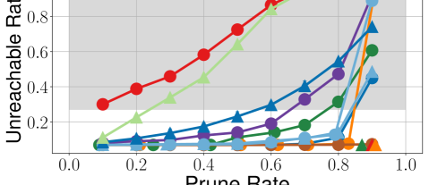
(a) Pair Unreachable Ratio

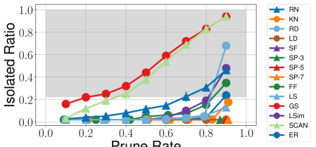
(b) Vertex Isolated Ratio

Figure 1. Graph Connectivity on ca-AstroPh.

Figures 1(a) and 1(b) show the source-destination pair unreachable ratio and vertex isolated ratio, respectively. As the prune rate increases, the graph becomes more disconnected, leading to an increase in isolated vertices. K-Neighbor excels at preserving graph connectivity because it ensures that each vertex retains at least $k$ edges. Two local sparsifiers, Local Degree and Local Similarity, also show strong performance since they both select edges to maintain locally, guaranteeing at least one edge for each vertex. ER performs well by retaining high-resistance edges, which are the low-redundancy edges crucial for maintaining graph connectivity. Spanning Forest and t-Spanners preserve the same level of connectivity as the original graph, as ensured by the algorithms. Random does not effectively preserve graph connectivity because it does not attempt to maintain edges critical for connectivity. G-Spar and SCAN retain edges connecting similar vertices on a global scale, and these edges are often intra-community edges that are not crucial for preserving connectivity, resulting in the poorest performance. The acceptable unreachable/isolated ratio can be customized according to specific applications. In this paper, we consider an increase of 20% or more in the unreachable/isolated ratio compared to the original graph as excessive (shown as the grey area in Figures 1(a) and 1(b)).

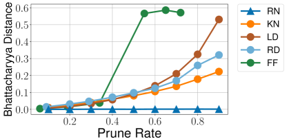
Figure 2. Degree distribution comparison on ogbn-proteins. Lower is better. Random performs the best, Local Degree and Forest Fire do not do well in preserving degree distribution.

Degree Distribution. Figure 2 illustrates the degree distribution on ogbn-proteins. A lower Bhattacharyya distance signifies a more similar degree distribution to the original graph. Random demonstrates the best performance in preserving the degree distribution. This is due to Random treats all edges without bias, thus maintaining the same proportion of edges for all vertices and keeping a similar degree distribution. Given that most graphs exhibit a power-law degree distribution, some sparsifiers struggle to preserve degree distribution. For instance, Local Degree and Rank Degree tend to retain edges connected to high-degree vertices. Conversely, K-Neighbor maintains up to K edges for all vertices, eliminating surplus edges from high-degree vertices. These biases negatively impact the preservation of the degree distribution. Among all sparsifiers, Random consistently performs well across all graphs, while Local Degree, Rank Degree, K-Neighbor, and Forest Fire under-perform on most graphs. The performance of other sparsifiers moderately fluctuates across graphs due to different graph characteristics.

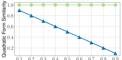
Figure 3. Laplacian quadratic form comparison of different sparsifiers on com-Amazon. Closer to 1 is better. ER-weighted performs the best. Random and other sparsifiers do not preserve Laplacian quadratic form.

Laplacian Quadratic Form. Figure 3 displays the Laplacian quadratic form similarity on com-Amazon. A value closer to 1 indicates better quality. From the figure, ER-weighted emerges as the clear winner. This is because the Laplacian quadratic form is the specific attribute ER-weighted is designed to preserve. Note that only ER-weighted possesses this property. ER-unweighted, along with other sparsifiers, exhibits no capability to preserve Laplacian quadratic form similarity at all, and they show the same pattern as Random. The pattern observed on com-Amazon is consistent across other undirected graphs. For directed graphs (not shown due to space limit), the Laplacian quadratic form ratio for ER-weighted is no longer guaranteed to be close to 1, this is because the symmetrization process deviates the graph’s spectral property from that of the original directed graph. However, ER-weighted still maintains a constant ratio and offers a better guarantee than other sparsifiers.

4.2. Distance Metrics

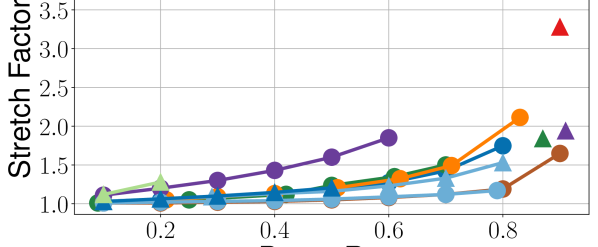
(a) Adjusted SPSP Stretch Factor

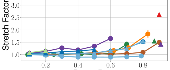
(b) Adjusted Eccentricity Stretch Factor

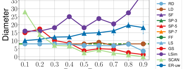
(c) Diameter

Figure 4. (a) Adjusted SPSP stretch factor of sparsifiers on ca-AstroPh with the constraint of acceptable pair unreachable ratio. (b) Adjusted eccentricity stretch factor of sparsifiers on ca-AstroPh with the constraint of acceptable vertex isolated ratio. (c) Diameter comparison on ego-Facebook. For stretch factor, closer to 1 is better. For graph diameter, closer to ground truth (green line) is better. Rank Degree and Local Degree have the best performance. G-Spar and SCAN do not perform well.

SPSP. A practical sparsifier should keep the mean stretch factor close to 1 while keeping the unreachable ratio relatively low. Figure 4(a) shows the mean stretch factor of 100,000 sampled source-destination pairs, with the constraint that the unreachable ratio is ¡20% over that in the original graph (white area in figure 1(a)). This allows for a comparison of the mean stretch factor without a significant increase in the number of unreachable pairs. Local Degree and Rank Degree demonstrate the best performance in preserving distances while maintaining a low unreachable ratio. This is because both of them are biased towards preserving edges of high-degree vertices, which are typically hub vertices in the graph and often lie along many shortest paths. L-Spar, ER-unweighted, Forest Fire, and K-Neighbor also exhibit strong performance due to their ability to maintain graph connectivity. Conversely, G-Spar and SCAN perform poorly as they rapidly increase the unreachable ratio and have a higher stretch factor. Although Spanning Forest and t-Spanners have a relatively high stretch factor, they guarantee the connectivity of the original graph, allowing them to maintain the unreachable ratio. t-Spanners fulfill the guarantee that the stretch factor is at most t but empirically show a higher mean stretch factor than Local Degree. t-Spanners is useful when connectivity is paramount and a slightly higher stretch factor is tolerable.

Eccentricity. Figure 4(b) presents the performance of sparsifiers with the vertex isolation ratio is ¡20% higher than that in the original graph (white area in figure 1(b)). Local Degree and Rank Degree perform the best in preserving eccentricity while keeping the unreachable ratio low. L-Spar, ER-unweighted, Forest Fire, and K-Neighbor also show strong performance due to their ability to maintain graph connectivity. G-Spar and SCAN perform poorly compared to other sparsifiers. Spanning Forest and t-Spanners have a relatively high stretch factor but guarantee the graph connectivity. Additionally, t-Spanners provide a theoretical upper bound on the stretch factor, making them suitable for certain scenarios.

Diameter. Figure 4(c) presents the diameters of various sparsified graphs at various prune rates. The green dashed line (8) indicates the diameter measured on the full graph as ground truth. We observe that Local Degree and Rank Degree perform the best, consistent with their strong performance in preserving distance. G-Spar, SCAN, and Local Similarity perform poorly compared to other sparsifiers.

In general, distance-related metrics are consistent across graphs. Some graphs (e.g., com-Amazon) have a lower average degree, causing the unreachable ratio or vertex isolation ratio to increase more quickly than in other graphs. Local Degree and Rank Degree consistently demonstrate the best performance for all distance-related metrics; however, Local Degree more effectively maintains the connectivity. G-Spar and SCAN always under-perform because they both tend to keep intra-community edges. This leads to a more disconnected graph and a high unreachable/isolation ratio.

4.3. Centrality Metrics

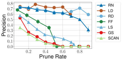
(a) Betweenness Centrality

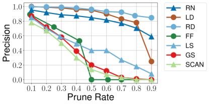
(b) Closeness Centrality

Figure 5. Top-100 precision for Betweenness and Closeness centrality. Higher is better. (a) Betweenness centrality on com-DBLP. (b) Closeness centrality on ca-AstroPh. Local Degree, Rank Degree, and Random have the best performance. L-Spar, G-Spar, SCAN, and Forest Fire do not perform well.

Betweenness and Closeness Centrality. Figure 5(a) and 5(b) display the top-100 precision of betweenness centrality on com-DBLP and closeness centrality on ca-AstroPh. Local Degree and Rank Degree exhibit the best performance. This is because the top-scored vertices are typically hub vertices, and as explained in § 4.2, both Local Degree and Rank Degree preserve edges incident to high-degree vertices, thus maintaining the betweenness and closeness ranking of hub vertices. Random uniformly samples edges without bias, and preserves the relative ranking to some extent. G-Spar and SCAN do not perform well as they aggressively disconnect graphs. We consistently observe Local Degree, Rank Degree, and Random perform well, and G-Spar and SCAN perform poorly across graphs.

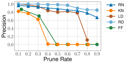
Figure 6. Eigenvector centrality top-100 precision comparison on email-Enron. Higher is better. Rank Degree and Random have the best performance. Forest Fire and K-Neighbor do not perform well.

Eigenvector Centrality. Figure 6 presents the top-100 precision of eigenvector centrality on email-Enron. Rank Degree achieves the best performance because it retains edges connected to high-degree vertices. Although eigenvector centrality is not directly linked to degree, high-degree vertices have a higher probability of being directly or indirectly (via n-hop neighbors) connected to important vertices. In comparison, Local Degree performs worse than Rank Degree since it only considers the degree of immediate neighbors and may disconnect vertices from vital vertices located more than 1-hop away. Random shows strong performance due to its unbiased nature, which helps preserve relative ranking. Both Forest Fire and K-Neighbor under-perform in preserving eigenvector centrality.

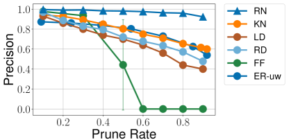
Figure 7. Katz centrality top-100 precision comparison of different sparsifiers on ego-Twitter. Higher is better. Random has the best performance. Forest Fire does not perform well.

Katz Centrality. Figure 7 illustrates the top-100 precision of Katz centrality on ego-Twitter. Random demonstrates the most effective performance. This is due to that Random proportionally maintains the number of edges relative to the original degree for all vertices. Thus, the graph’s hop structure closely resembles its original state. Empirically, K-Neighbor and ER-unweighted also exhibit strong performance. Local Degree and Rank Degree do not perform well since they solely focus on degree, thereby only accounting for immediate neighbors. Therefore, vertices with low-degree immediate neighbors but high k-hop (k¿1) neighbors are severely penalized. Minor fluctuations in sparsifiers’ relative performance on certain graphs can be attributed to the variation in the attenuation factor $\alpha$. Overall, the performance is consistent across graphs.

In summary, Local Degree, Rank Degree, and Random consistently excel in centrality-related metrics. This is because Local Degree and Rank Degree retain edges connected to hub vertices, and centrality metrics seek important vertices in the graph, which often correspond to hub vertices. Conversely, Random maintains edges without bias, thus effectively preserving the relative vertex ranking.

4.4. Clustering Metrics

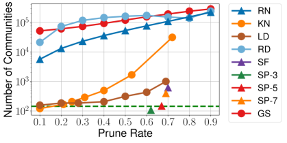
Figure 8. Number of communities comparison on com-DBLP. Closer to the green line is better. Local Degree, Spanning Forest, and t-Spanners have the best performance. G-Spar, Rank Degree, and Random do not perform well.

Number of Communities. We employ the widely recognized Louvain method (Blondel et al., 2008) for community detection, assuming the number of communities is unknown, and use the number detected in the original graph as the ground truth. Figure 8 presents a comparison of community numbers on com-DBLP, with the green dashed line representing the ground truth; the closer to it, the better. As the prune rate increases, the graph becomes increasingly disconnected, and the number of communities consistently rises. Local Degree and K-Neighbor excel in maintaining the community number relatively close to the ground truth because it preserves the connectivity. Spanning Forest and t-Spanners also demonstrate strong performance, surpassing Local Degree at equivalent prune rates, as they ensure connectivity remains identical to the original graph. Unlike Local Degree, Rank Degree struggles to preserve the community number because it sparsifies globally without providing guarantees on connectivity preservation. In various graphs, Local Degree, Spanning Forest, and t-Spanners consistently outperform.

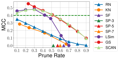
(a) Mean clustering coefficient.

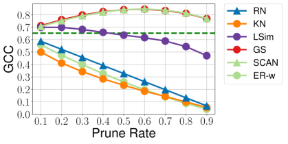
(b) Global clustering coefficient.

Figure 9. Clustering coefficients comparison. Closer to the green line is better. (a) shows the MCC on com-Amazon (b) shows the GCC on human_gene2. No sparsifier is effective in preserving the clustering coefficient.

Clustering Coefficient. Figure 9 compares clustering coefficients on com-Amazon and human_gene2. We use the mean clustering coefficient (MCC) to evaluate the local clustering coefficient (LCC), as it represents the average LCC of all vertices. The green dashed lines indicate the MCC and GCC of the original graph. Generally, most sparsifiers exhibit decreasing MCC and GCC as the prune rate rises, with only Local Similarity, SCAN, and G-Spar exhibiting slight increases in MCC at lower prune rates. None of the sparsifiers demonstrate outstanding performance in preserving MCC and GCC, as they all degrade linearly with respect to the prune rate. Spanning Forest and t-Spanners consistently have an MCC of 0 due to the absence of loops in the graph. Clustering coefficient results vary across different graphs, with graph categories and directedness significantly impacting sparsifier performance. Overall, no sparsifier proves effective in preserving clustering coefficients.

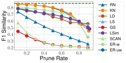
Figure 10. Clustering F1 similarity comparison of different sparsifiers on ca-HepPh. Higher is better. ER-unweighted, ER-weighted, K-Neighbor, Local Degree, L-Spar, and Local Similarity perform the best. SCAN and G-Spar underperform.

Clustering F1 Similarity. Relying solely on the number of communities to evaluate clustering quality is insufficient, therefore, we employ the clustering F1 score to measure clustering similarity (see § 2.2.4). Figure 10 shows the clustering F1 similarity comparison on ca-HepPh, with F1 similarity ranging from 0 (worst) to 1 (best). The green dashed line represents the clustering F1 similarity when applying clustering algorithms twice on the original graph; it is not 1 due to the inherent randomness in the clustering algorithm. For all sparsifiers, F1 similarity decreases as the prune rate increases. K-Neighbor exhibits the best overall performance, while Local Similarity, Local Degree, and L-Spar also demonstrate strong results. These sparsifiers share a focus on local edges, and locally similar vertices more likely to belong to the same community. Empirically, we also observe that ER-weighted and ER-unweighted perform well, potentially due to ER’s preservation of low-redundant edges, which are often crucial in clustering algorithms. In contrast, G-Spar and SCAN display poor performance in preserving clustering similarity. Across graphs, K-Neighbor, Local Degree, Local Similarity, L-Spar, ER-unweighted, and ER-weighted consistently rank as top performers, while G-Spar and SCAN persistently underperform.

4.5. High-level Metrics

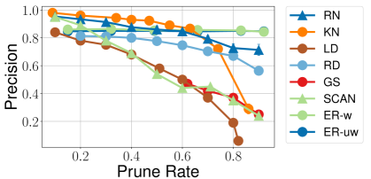
(a) PageRank Centrality on web-Google

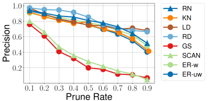
(b) PageRank Centrality on ego-Facebook

Figure 11. PageRank centrality. Higher precision is better. (a) PageRank centrality on web-Google. K-Neighbor and Random perform the best at a low prune rate, ER-weighted and ER-unweighted perform the best at a high prune rate. Local Degree, G-Spar, and SCAN do not perform well. (b) PageRank centrality on ego-Facebook. Rank Degree has the best performance. G-Spar and SCAN underperform.

PageRank. Figures 11(a) and  11(b) present the top-100 precision of PageRank on web-Google and ego-Facebook, respectively. Note that web-Google is a directed graph and ER only supports undirected graphs. Thus, we symmetrize the graph before performing ER. Sparsifiers that work on directed graphs are applied directly.

As illustrated in Figure 11(a), ER-unweighted and ER-weighted demonstrate high precision and consistency at various prune rates. On all web networks (web-NotreDame, web-BerkStan, web-Google, web-Stanford) the performance of ER remains similar in that precision is almost constant at different prune rates. However, ER does not always achieve the best performance at low prune rates. For some graphs, the precision of ER remains constant but at a lower level. This can be due to the symmetrizing process altering the original graph’s information. The more symmetrical the original graph is, the less influence will be introduced. K-Neighbor also shows good performance at low prune rates. In contrast, G-Spar, SCAN, and Local Degree fail to preserve PageRank effectively.

Figure 11(b) reveals ER sparsifier’s performance on unweighted graphs, using ego-Facebook as an example. Rank Degree, Local Degree, Random, K-Neighbor, ER-unweighted, and ER-weighted all exhibit similar performance in preserving PageRank. G-Spar and SCAN continue to underperform. In comparison to directed graphs, ER no longer exhibits almost constant precision at varying prune rates on undirected graphs. Rank Degree and K-Neighbor consistently perform well on both directed and undirected graphs. Local Degree displays a significant discrepancy in performance between directed and undirected graphs, excelling in undirected graphs but consistently underperforming in directed ones. G-Spar and SCAN show poor performance consistently.

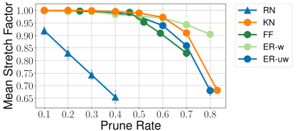
Figure 12. Adjusted Mean Stretch Factor for min-cut/max-flow with the constraint of acceptable unreachable ratio on ca-HepPh. Closer to 1 is better. ER-weighted has the best performance.

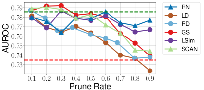
(a) GraphSAGE comparison of different sparsifiers on ogbn-proteins

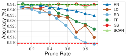
(b) ClusterGCN comparison of different sparsifiers on Reddit

Figure 13. GNN comparison of different sparsifiers. Higher AUROC and accuracy are better. The green line represents the inference results on the model trained by the full graph. The red line represents the inference results on the model trained with no graph (MLP only). (a) is evaluated with the GraphSAGE on ogbn-proteins. (b) is evaluated with the ClusterGCN on Reddit.

Min-cut/Max-flow. Figure 12 presents the mean stretch factor on ca-HepPh, with the constraint that the unreachable ratio remains ¡20% higher than in the original graph. A mean stretch factor closer to 1 means better performance. ER-weighted shows the best performance. This can be attributed to ER being a spectral sparsifier, which preserves the spectral properties of graphs (Spielman and Srivastava, 2011). Min-cut/max-flow methods are also closely related to the graph spectrum. Flow-based graph partitioning (Ng et al., 2001) employs the Fiedler vector (Fiedler, 1973) (eigenvector corresponding to the second smallest eigenvalue of the graph Laplacian). One can intuitively think of ER as retaining high-resistance (low-redundant) edges in the graph, which are typically found in the critical (narrowest) section of the max-flow problem. ER-weighted significantly outperforms its unweighted counterpart ER-unweighted, as ER-weighted effectively compensates for the weights of other edges when removing edges. K-Neighbor and Forest Fire show good empirical performance as well. In contrast, G-Spar and SCAN underperform, and other sparsifiers exhibit similarly mediocre results. The outcomes for min-cut/max-flow are consistent across graphs, with ER-weighted as the top performer, followed by K-Neighbor and Forest Fire.

GNN. Figures 13(a) and 13(b) show the performance of sparsifiers on two distinct GNN models. GNN performance is measured using AUROC and/or vertex classification accuracy. The green dashed line represents performance on the full graph, while the red dashed line represents performance on the empty graph (a graph with no edges). We include the empty graph to demonstrate the performance of GNN models based solely on vertex features without any graph structural information. On the GraphSAGE model, Random and Local Similarity perform the best; G-Spar and SCAN show good performance at low prune rates but deteriorate rapidly at higher rates. However, on the CluterGCN model, G-Spar and SCAN perform well at all prune rates. Local Degree and Rank Degree consistently underperform compared to other sparsifiers on both models. Due to the complexity of GNN algorithms, it is challenging to draw straightforward conclusions. Overall, the performance of sparsifiers on GNNs differs from model to model, which may be due to the inherent characteristics of GNN workloads.

4.6. Sparsification Time

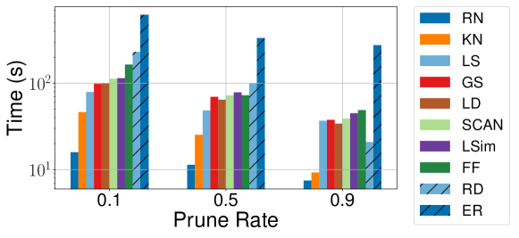
Figure 14. Sparsification time comparison on ogbn-proteins

Figure 14 shows the sparsification time of different sparsifiers at different prune levels. For all sparsifiers, sparsification time decreases as the prune rate increases, this is expected because the higher the prune rate, the fewer edges need to be picked. Across sparsifiers, the sparsification time is also different. Random and K-Neighbor are the sparsifiers with the lowest overhead due to their low algorithmic complexity. L-Spar, G-Spar, Local Degree, SCAN, Local Similarity, Forest Fire, and Rank Degree show similar latency. ER is the most complex algorithm. In the figure, the time for ER is only for sampling. We do not include the computation time of the effective resistance because it is a one-time cost. The computation of effective resistance takes 990 seconds for ogbn-proteins. and the execution time of ER is approximately an order of magnitude higher than that of other sparsifiers. However, depending on the application, a high-cost sparsifier like ER can still be useful if it preserves the desired graph properties, and the sparsification overhead is less than the time that can be saved in performing the downstream task on the sparsified graph.

4.7. Summary of Results and Insights

Overall, The performance of all sparsifiers degrades as the prune rate increases. Usually, we observe that the relative performance of sparsifiers is consistent across prune rates, meaning superior sparsifiers at low prune rates will remain superior at high prune rates, and the performance gap between the superiors and inferiors will be larger. On some occasions, the performance of a sparsifier have an elbow point, beyond which the performance drops sharply. This is due to some sparsifiers unable to maintain certain property beyond a the elbow prune rate. For example, in figure 6, the performance of Local Degree dropped abruptly when increasing the prune rate from 0.8 to 0.9, because the number of edge is so low that it cannot maintain the graph connectivity anymore.

To make sparsification effective, the selection of the sparsification algorithm should preserve the graph property/properties on which the downstream application is based. We summarize the what each sparsifier preserve below.

• Random: preserves relative (distribution-based or ranking-based) properties, for example, degree distribution, and top centrality rankings. It struggles to preserve absolute (valued-based) properties, for example, number of communities, clustering coefficient, and min-cut/max-flow.

• K-Neighbor, Spanning Forest, and t-Spanners: preserves graph connectivity; keeps pair unreachable ratio and vertex isolated ratio low.

• Rank Degree and Local Degree: preserves graph connectivity and edges to high-degree vertices (hub vertices). Perform well on distance metrics (APSP, eccentricity, diameter) and centrality metrics.

• Forest Fire: simulates the evolution of graphs and does not strictly stick to the original graph. Empirically it does not excel at any metrics evaluated.

• G-Spar and SCAN: Empirically perform well in preserving ClusterGCN accuracy.

• L-Spar and Local Similarity: preserves the edge to similar vertices, thus preserves clustering similarity.

• ER: preserves the spectral properties of the graph, specifically the quadratic form of the graph Laplacian. It perform well in preserving min-cut/max-flow results.

5. Related Work

ML-based sparsifiers are a group of sparsifiers that use machine learning-related techniques to sparsify graphs. SparRL (Wickman et al., 2022) proposes a graph sparsification framework enabled by deep reinforcement learning. NeuralSparse (Zheng et al., 2020) presents a supervised graph sparsification technique to improve performance in graph neural networks (GNN). Instead of focusing on saving execution time by performing graph sparsification, NeuralSparse aims to remove task-irrelevant edges from the graph, and thus improve the accuracy of the downstream GNNs. DropEdge (Rong et al., 2019) presents a method very close to the random sparsifier, but samples a random set of edges for each training epoch in graph convolutional network (GCN), the goal is both to reduce message passing overhead and reduce over-fitting with the full graph input.

6. Conclusion

This study provides a comprehensive evaluation of 12 graph sparsification algorithms, analyzing their performance in preserving 16 essential graph metrics across 14 real-world graphs with diverse characteristics. Our findings revealed that no single sparsifier excels in preserving all graph properties, and it is important to select appropriate sparsification algorithms based on the downstream task. This study contributes to the broader understanding of graph sparsification algorithms, and we provided insights to guide future work in effectively integrating graph sparsification into graph algorithms to optimize computational efficiency without significantly compromising output quality. Our open-source framework offers a valuable resource for ongoing evaluations of emerging sparsification algorithms, graph metrics, and growing graph data.

- (1)
- wik (2022a) 2022a. Spanning Tree. https://en.wikipedia.org/wiki/Spanning_tree (last accessed date: 11/15/2023).
- wik (2022b) 2022b. Tree (graph theory). https://en.wikipedia.org/wiki/Tree_(graph_theory) (last accessed date: 11/15/2023).
- wik (2023a) 2023a. Clustering coefficient. https://en.wikipedia.org/wiki/Clustering_coefficient (last accessed date: 11/15/2023).
- wol (2023) 2023. Connected graph. https://mathworld.wolfram.com/ConnectedGraph.html (last accessed date: 11/15/2023).
- wik (2023b) 2023b. Cut (graph theory). https://en.wikipedia.org/wiki/Cut_(graph_theory) (last accessed date: 11/15/2023).
- Wik (2023) 2023. Eigenvector centrality. https://en.wikipedia.org/wiki/Eigenvector_centrality (last accessed date: 11/15/2023).
- Ahuja et al. (1993) Ravindra K. Ahuja, Thomas L. Magnanti, and James B. Orlin. 1993. Network Flows: Theory, Algorithms, and Applications. Prentice-Hall, Inc., USA.
- Althöfer et al. (1990) Ingo Althöfer, Gautam Das, David Dobkin, and Deborah Joseph. 1990. Generating sparse spanners for weighted graphs. In SWAT 90, John R. Gilbert and Rolf Karlsson (Eds.). Springer Berlin Heidelberg, Berlin, Heidelberg, 26–37.
- Belkin and Niyogi (2001) Mikhail Belkin and Partha Niyogi. 2001. Laplacian Eigenmaps and Spectral Techniques for Embedding and Clustering. In Advances in Neural Information Processing Systems, T. Dietterich, S. Becker, and Z. Ghahramani (Eds.), Vol. 14. MIT Press. https://proceedings.neurips.cc/paper_files/paper/2001/file/f106b7f99d2cb30c3db1c3cc0fde9ccb-Paper.pdf
- Bergamini et al. (2017) Elisabetta Bergamini, Michele Borassi, Pierluigi Crescenzi, Andrea Marino, and Henning Meyerhenke. 2017. Computing top-k Closeness Centrality Faster in Unweighted Graphs. arXiv:1704.01077 [cs.DS]
- Bhattacharyya (1946) A. Bhattacharyya. 1946. On a Measure of Divergence between Two Multinomial Populations. Sankhyā: The Indian Journal of Statistics (1933-1960) 7, 4 (1946), 401–406. http://www.jstor.org/stable/25047882
- Blondel et al. (2008) Vincent D Blondel, Jean-Loup Guillaume, Renaud Lambiotte, and Etienne Lefebvre. 2008. Fast unfolding of communities in large networks. Journal of Statistical Mechanics: Theory and Experiment 2008, 10 (oct 2008), P10008. https://doi.org/10.1088/1742-5468/2008/10/p10008
- Boeing (2018) Geoff Boeing. 2018. Measuring the Complexity of Urban Form and Design. Urban Design International 23 (11 2018), 281–292. https://doi.org/10.1057/s41289-018-0072-1
- Bondy and Murty (1976) J. A. Bondy and U. S. R. Murty. 1976. Graph Theory with Applications. Elsevier, New York.
- Brin and Page (1998) Sergey Brin and Lawrence Page. 1998. The Anatomy of a Large-Scale Hypertextual Web Search Engine. Computer Networks 30 (1998), 107–117. http://www-db.stanford.edu/~backrub/google.html
- BURT (1992) RONALD S. BURT. 1992. Structural Holes: The Social Structure of Competition. http://www.jstor.org/stable/j.ctv1kz4h78.
- Chen et al. (2023) Yuhan Chen, Alireza Khadem, Xin He, Nishil Talati, Tanvir Ahmed Khan, and Trevor Mudge. 2023. PEDAL: A Power Efficient GCN Accelerator with Multiple DAtafLows. In Proceedings of the 26th Design, Automation, and Test in Europe (DATE) conference (DATE 2023).
- Curtis et al. (2011) Andrew R. Curtis, Tommy Carpenter, and S. Keshav. 2011. REWIRE: An Optimization-based Framework for Data Center Network Design. (2011).
- Davis and Hu (2011) Timothy A. Davis and Yifan Hu. 2011. The University of Florida Sparse Matrix Collection. ACM Trans. Math. Softw. 38, 1, Article 1 (dec 2011), 25 pages. https://doi.org/10.1145/2049662.2049663
- Defferrard et al. (2016) Michaël Defferrard, Xavier Bresson, and Pierre Vandergheynst. 2016. Convolutional Neural Networks on Graphs with Fast Localized Spectral Filtering. (2016). https://doi.org/10.48550/ARXIV.1606.09375
- Demir et al. (2021) Andac Demir, Toshiaki Koike-Akino, Ye Wang, Masaki Haruna, and Deniz Erdogmus. 2021. EEG-GNN: Graph Neural Networks for Classification of Electroencephalogram (EEG) Signals. In 2021 43rd Annual International Conference of the IEEE Engineering in Medicine & Biology Society (EMBC). 1061–1067. https://doi.org/10.1109/EMBC46164.2021.9630194
- Dijkstra (1959) E. W. Dijkstra. 1959. A Note on Two Problems in Connexion with Graphs. Numer. Math. 1, 1 (dec 1959), 269–271. https://doi.org/10.1007/BF01386390
- Draves et al. (2004) Richard Draves, Jitendra Padhye, and Brian Zill. 2004. Comparison of Routing Metrics for Static Multi-Hop Wireless Networks. SIGCOMM Comput. Commun. Rev. 34, 4 (aug 2004), 133–144. https://doi.org/10.1145/1030194.1015483
- Ester et al. (1996) Martin Ester, Hans-Peter Kriegel, Jörg Sander, and Xiaowei Xu. 1996. A Density-Based Algorithm for Discovering Clusters in Large Spatial Databases with Noise. In Proceedings of the Second International Conference on Knowledge Discovery and Data Mining (Portland, Oregon) (KDD’96). AAAI Press, 226–231.
- Fawcett (2006) Tom Fawcett. 2006. An introduction to ROC analysis. Pattern Recognition Letters 27, 8 (2006), 861–874. https://doi.org/10.1016/j.patrec.2005.10.010 ROC Analysis in Pattern Recognition.
- Fey and Lenssen (2019) Matthias Fey and Jan Eric Lenssen. 2019. Fast Graph Representation Learning with PyTorch Geometric. CoRR abs/1903.02428 (2019). arXiv:1903.02428
- Fiedler (1973) Miroslav Fiedler. 1973. Algebraic connectivity of graphs. Czechoslovak Mathematical Journal 23, 2 (1973), 298–305. http://eudml.org/doc/12723
- Fletcher and Wennekers (2018) Jack McKay Fletcher and Thomas Wennekers. 2018. From structure to activity: Using centrality measures to predict neuronal activity. International Journal of Neural Systems 28, 02 (2018), 1750013. https://doi.org/10.1142/s0129065717500137
- Ford and Fulkerson (1956) L. R. Ford and D. R. Fulkerson. 1956. Maximal Flow Through a Network. Canadian Journal of Mathematics 8 (1956), 399–404. https://doi.org/10.4153/CJM-1956-045-5
- Freeman (2004) Linton Freeman. 2004. The Development of Social Network Analysis. (01 2004).
- Geisberger et al. (2008) Robert Geisberger, Peter Sanders, and Dominik Schultes. 2008. Better Approximation of Betweenness Centrality. In Proceedings of the Meeting on Algorithm Engineering & Expermiments (San Francisco, California). Society for Industrial and Applied Mathematics, USA, 90–100.
- Hahn and Kern (2004) Matthew W. Hahn and Andrew D. Kern. 2004. Comparative Genomics of Centrality and Essentiality in Three Eukaryotic Protein-Interaction Networks. Molecular Biology and Evolution 22, 4 (12 2004), 803–806. https://doi.org/10.1093/molbev/msi072 arXiv:https://academic.oup.com/mbe/article-pdf/22/4/803/13433323/msi072.pdf
- Hamann et al. (2016) Michael Hamann, Gerd Lindner, Henning Meyerhenke, Christian L. Staudt, and Dorothea Wagner. 2016. Structure-Preserving Sparsification Methods for Social Networks. arXiv:1601.00286 [cs.SI]
- Hamilton et al. (2017) William L. Hamilton, Rex Ying, and Jure Leskovec. 2017. Inductive Representation Learning on Large Graphs. In Proceedings of the 31st International Conference on Neural Information Processing Systems (Long Beach, California, USA) (NIPS’17). Curran Associates Inc., Red Hook, NY, USA, 1025–1035.
- Hu et al. (2020) Weihua Hu, Matthias Fey, Marinka Zitnik, Yuxiao Dong, Hongyu Ren, Bowen Liu, Michele Catasta, and Jure Leskovec. 2020. Open Graph Benchmark: Datasets for Machine Learning on Graphs. arXiv preprint arXiv:2005.00687 (2020).
- Jeong et al. (2000) H. Jeong, B. Tombor, R. Albert, Z. N. Oltvai, and A.-L. Barabási. 2000. The large-scale organization of metabolic networks. Nature 407, 6804 (oct 2000), 651–654. https://doi.org/10.1038/35036627
- Katz (1953) Leo Katz. 1953. A new status index derived from sociometric analysis. Psychometrika 18 (1953), 39–43.
- Kipf and Welling (2016) Thomas N. Kipf and Max Welling. 2016. Semi-Supervised Classification with Graph Convolutional Networks. https://doi.org/10.48550/ARXIV.1609.02907
- Kruskal (1956) Joseph B. Kruskal. 1956. On the shortest spanning subtree of a graph and the traveling salesman problem.
- Leskovec et al. (2006) Jure Leskovec, Jon M. Kleinberg, and Christos Faloutsos. 2006. Graph evolution: Densification and shrinking diameters. ACM Trans. Knowl. Discov. Data 1 (2006), 2.
- Leskovec and Krevl (2014) Jure Leskovec and Andrej Krevl. 2014. SNAP Datasets: Stanford Large Network Dataset Collection. http://snap.stanford.edu/data.
- Li et al. (2019) Zekun Li, Zeyu Cui, Shu Wu, Xiaoyu Zhang, and Liang Wang. 2019. Fi-GNN: Modeling Feature Interactions via Graph Neural Networks for CTR Prediction. In Proceedings of the 28th ACM International Conference on Information and Knowledge Management (Beijing, China) (CIKM ’19). Association for Computing Machinery, New York, NY, USA, 539–548. https://doi.org/10.1145/3357384.3357951
- Lloyd (1982) S. Lloyd. 1982. Least squares quantization in PCM. IEEE Transactions on Information Theory 28, 2 (1982), 129–137. https://doi.org/10.1109/TIT.1982.1056489
- Luce and Perry (1949) R. Duncan Luce and Albert D. Perry. 1949. A method of matrix analysis of group structure. Psychometrika 14 (1949), 95–116.
- Ma and Zeng (2003) Hong-Wu Ma and An-Ping Zeng. 2003. The connectivity structure, giant strong component and centrality of metabolic networks. Bioinformatics 19, 11 (07 2003), 1423–1430. https://doi.org/10.1093/bioinformatics/btg177
- Magoni and Pansiot (2001) Damien Magoni and Jean Jacques Pansiot. 2001. Analysis of the Autonomous System Network Topology. SIGCOMM Comput. Commun. Rev. 31, 3 (jul 2001), 26–37. https://doi.org/10.1145/505659.505663
- Mallawaarachchi (2020) Vijini Mallawaarachchi. 2020. Evaluating clustering results. https://towardsdatascience.com/evaluating-clustering-results-f13552ee7603
- Murphy (1996) Allan H. Murphy. 1996. The Finley Affair: A Signal Event in the History of Forecast Verification. Weather and Forecasting 11, 1 (1996), 3 – 20. https://doi.org/10.1175/1520-0434(1996)011<0003:TFAASE>2.0.CO;2
- Müllner (2011) Daniel Müllner. 2011. Modern hierarchical, agglomerative clustering algorithms. https://doi.org/10.48550/ARXIV.1109.2378
- Newman (2004) Mark EJ Newman. 2004. Coauthorship networks and patterns of scientific collaboration. Proceedings of the national academy of sciences 101, suppl_1 (2004), 5200–5205.
- Newman (2016) M. E. J. Newman. 2016. Mathematics of Networks. Palgrave Macmillan UK, London, 1–8. https://doi.org/10.1057/978-1-349-95121-5_2565-1
- Ng et al. (2001) Andrew Y. Ng, Michael I. Jordan, and Yair Weiss. 2001. On Spectral Clustering: Analysis and an Algorithm. In Proceedings of the 14th International Conference on Neural Information Processing Systems: Natural and Synthetic (Vancouver, British Columbia, Canada) (NIPS’01). MIT Press, Cambridge, MA, USA, 849–856.
- Page et al. (1999) Lawrence Page, Sergey Brin, Rajeev Motwani, and Terry Winograd. 1999. The PageRank Citation Ranking : Bringing Order to the Web. In The Web Conference.
- Pavlopoulos et al. (2011) Georgios A Pavlopoulos, Maria Secrier, Charalampos N Moschopoulos, Theodoros G Soldatos, Sophia Kossida, Jan Aerts, Reinhard Schneider, and Pantelis G Bagos. 2011. Using graph theory to analyze biological networks. BioData mining 4 (2011), 1–27.
- Peixoto (2014) Tiago P. Peixoto. 2014. The graph-tool python library. figshare (2014). https://doi.org/10.6084/m9.figshare.1164194
- Prim (1957) Robert C. Prim. 1957. Shortest connection networks and some generalizations. Bell System Technical Journal 36 (1957), 1389–1401.
- Ramesh et al. (2017) Varun Ramesh, Shivanee Nagarajan, Jason J. Jung, and Saswati Mukherjee. 2017. Max-flow min-cut algorithm with application to road networks. Concurrency and Computation: Practice and Experience 29, 11 (2017), e4099. https://doi.org/10.1002/cpe.4099 arXiv:https://onlinelibrary.wiley.com/doi/pdf/10.1002/cpe.4099 e4099 cpe.4099.
- Rapanos (2023) Theodoros Rapanos. 2023. What makes an opinion leader: Expertise vs popularity. Games and Economic Behavior 138 (2023), 355–372. https://doi.org/10.1016/j.geb.2023.01.003
- Richard C. Larsona (1981) Amedeo R. Odoni Richard C. Larsona. 1981. Urban operations research. (1981).
- Rong et al. (2019) Yu Rong, Wenbing Huang, Tingyang Xu, and Junzhou Huang. 2019. DropEdge: Towards Deep Graph Convolutional Networks on Node Classification. https://doi.org/10.48550/ARXIV.1907.10903
- Sadhanala et al. (2016) Veeranjaneyulu Sadhanala, Yu-Xiang Wang, and Ryan J. Tibshirani. 2016. Graph Sparsification Approaches for Laplacian Smoothing. In International Conference on Artificial Intelligence and Statistics.
- Satuluri et al. (2011) Venu Satuluri, Srinivasan Parthasarathy, and Yiye Ruan. 2011. Local Graph Sparsification for Scalable Clustering. In Proceedings of the 2011 ACM SIGMOD International Conference on Management of Data (Athens, Greece) (SIGMOD ’11). Association for Computing Machinery, New York, NY, USA, 721–732. https://doi.org/10.1145/1989323.1989399
- Scarselli et al. (2009) Franco Scarselli, Marco Gori, Ah Chung Tsoi, Markus Hagenbuchner, and Gabriele Monfardini. 2009. The Graph Neural Network Model. IEEE Transactions on Neural Networks 20, 1 (2009), 61–80. https://doi.org/10.1109/TNN.2008.2005605
- Scheurer and Porta (2006) Jan Scheurer and Sergio Porta. 2006. Centrality and Connectivity in Public Transport Networks and their Significance for Transport Sustainability in Cities. (07 2006).
- Song et al. (2018) L. Song, Y. Zhuo, X. Qian, H. Li, and Y. Chen. 2018. GraphR: Accelerating Graph Processing Using ReRAM. In 2018 IEEE International Symposium on High Performance Computer Architecture (HPCA). IEEE Computer Society, Los Alamitos, CA, USA, 531–543. https://doi.org/10.1109/HPCA.2018.00052
- Spielman (2023) Daniel Spielman. 2023. Laplacians.jl. https://github.com/danspielman/Laplacians.jl.
- Spielman and Srivastava (2011) Daniel A. Spielman and Nikhil Srivastava. 2011. Graph Sparsification by Effective Resistances. SIAM J. Comput. 40, 6 (2011), 1913–1926. https://doi.org/10.1137/080734029 arXiv:https://doi.org/10.1137/080734029
- Staudt et al. (2014) Christian L. Staudt, Aleksejs Sazonovs, and Henning Meyerhenke. 2014. NetworKit: A Tool Suite for Large-scale Complex Network Analysis. https://doi.org/10.48550/ARXIV.1403.3005
- Szklarczyk et al. (2018) Damian Szklarczyk, Annika Gable, David Lyon, Alexander Junge, Stefan Wyder, Jaime Huerta-Cepas, Milan Simonovic, Nadezhda Doncheva, John Morris, Peer Bork, Lars Jensen, and Christian von Mering. 2018. STRING v11: protein-protein association networks with increased coverage, supporting functional discovery in genome-wide experimental datasets. Nucleic acids research 47 (11 2018). https://doi.org/10.1093/nar/gky1131
- Takes and Kosters (2013) Frank W. Takes and Walter A. Kosters. 2013. Computing the Eccentricity Distribution of Large Graphs. Algorithms 6, 1 (2013), 100–118. https://doi.org/10.3390/a6010100
- Talati et al. (2022) N. Talati, H. Ye, S. Vedula, K. Chen, Y. Chen, D. Liu, Y. Yuan, D. Blaauw, A. Bronstein, T. Mudge, and R. Dreslinski. 2022. Mint: An Accelerator For Mining Temporal Motifs. In 2022 55th IEEE/ACM International Symposium on Microarchitecture (MICRO). IEEE Computer Society, Los Alamitos, CA, USA, 1270–1287. https://doi.org/10.1109/MICRO56248.2022.00089
- Veličković et al. (2017) Petar Veličković, Guillem Cucurull, Arantxa Casanova, Adriana Romero, Pietro Liò, and Yoshua Bengio. 2017. Graph Attention Networks. https://doi.org/10.48550/ARXIV.1710.10903
- Voudigari et al. (2016) Elli Voudigari, Nikos Salamanos, Theodore Papageorgiou, and Emmanuel J. Yannakoudakis. 2016. Rank degree: An efficient algorithm for graph sampling. In 2016 IEEE/ACM International Conference on Advances in Social Networks Analysis and Mining (ASONAM). 120–129. https://doi.org/10.1109/ASONAM.2016.7752223
- Watts and Strogatz (1998) Duncan J. Watts and Steven H. Strogatz. 1998. Collective dynamics of ‘small-world’ networks. Nature 393, 6684 (1998), 440–442. https://doi.org/10.1038/30918
- Wickman et al. (2022) R. Wickman, X. Zhang, and W. Li. 2022. A Generic Graph Sparsification Framework using Deep Reinforcement Learning. In 2022 IEEE International Conference on Data Mining (ICDM). IEEE Computer Society, Los Alamitos, CA, USA, 1221–1226. https://doi.org/10.1109/ICDM54844.2022.00158
- Xu et al. (2007) Xiaowei Xu, Nurcan Yuruk, Zhidan Feng, and Thomas A. J. Schweiger. 2007. SCAN: A Structural Clustering Algorithm for Networks. In Proceedings of the 13th ACM SIGKDD International Conference on Knowledge Discovery and Data Mining (San Jose, California, USA) (KDD ’07). Association for Computing Machinery, New York, NY, USA, 824–833. https://doi.org/10.1145/1281192.1281280
- Zheng et al. (2020) Cheng Zheng, Bo Zong, Wei Cheng, Dongjin Song, Jingchao Ni, Wenchao Yu, Haifeng Chen, and Wei Wang. 2020. Robust Graph Representation Learning via Neural Sparsification. In Proceedings of the 37th International Conference on Machine Learning (Proceedings of Machine Learning Research), Hal Daumé III and Aarti Singh (Eds.), Vol. 119. PMLR, 11458–11468. https://proceedings.mlr.press/v119/zheng20d.html
- Zhou et al. (2019) Fan Zhou, Chengtai Cao, Kunpeng Zhang, Goce Trajcevski, Ting Zhong, and Ji Geng. 2019. Meta-GNN: On Few-Shot Node Classification in Graph Meta-Learning. In Proceedings of the 28th ACM International Conference on Information and Knowledge Management (Beijing, China) (CIKM ’19). Association for Computing Machinery, New York, NY, USA, 2357–2360. https://doi.org/10.1145/3357384.3358106